
LinkNet-Spectral-Spatial-Temporal Transformer Based on Few-Shot Learning for Mangrove Loss Detection with Small Dataset

 ,
,  ,
,  ,
, 

Abstract
1. Introduction
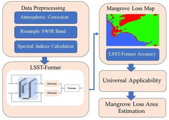
- A LSST-Former method is proposed for an improved deep-learning model that only requires a few labeled samples by innovatively combining the FCN algorithm with a transformer and incorporating spatial, spectral, and temporal data from Sentinel-2 images to detect mangrove loss.
- Experimental results strongly demonstrate the exceptional efficacy of our approach compared to other current models.
- An analysis of the universal applicability of LSST-Transformer algorithms across different locations of the mangrove ecosystem is given.
2. Materials and Methods
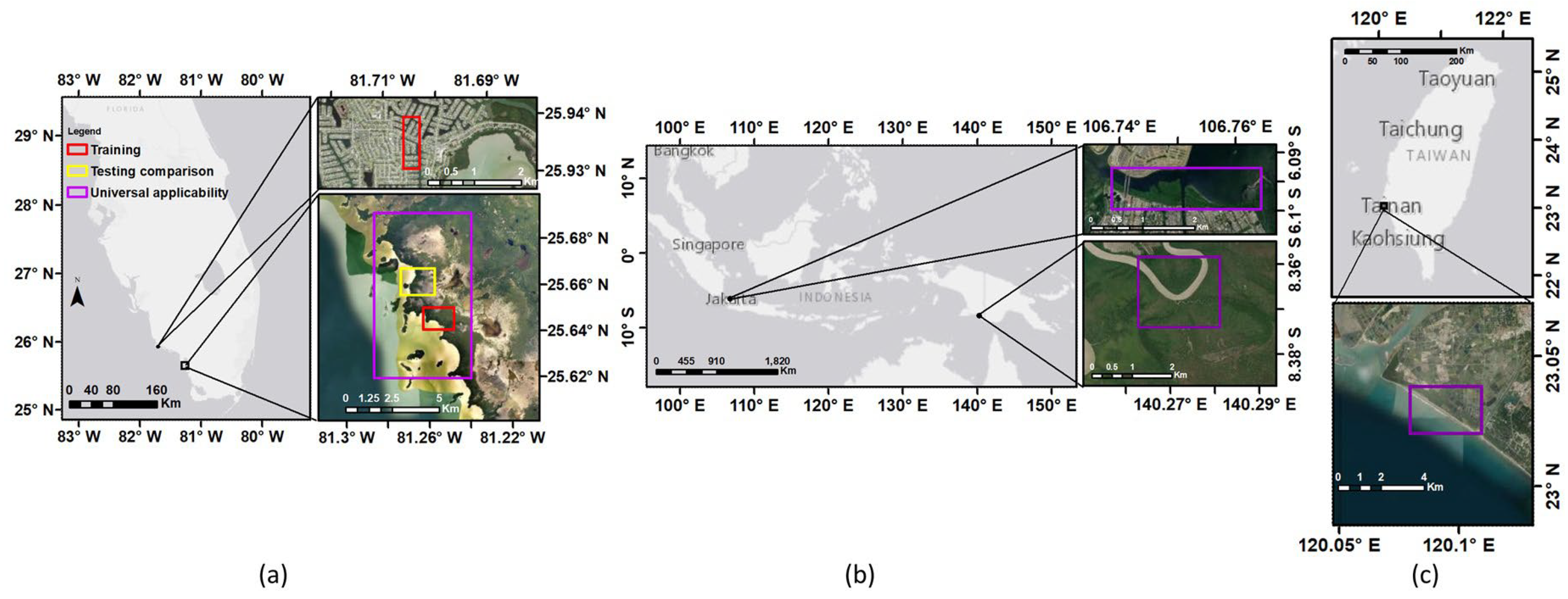
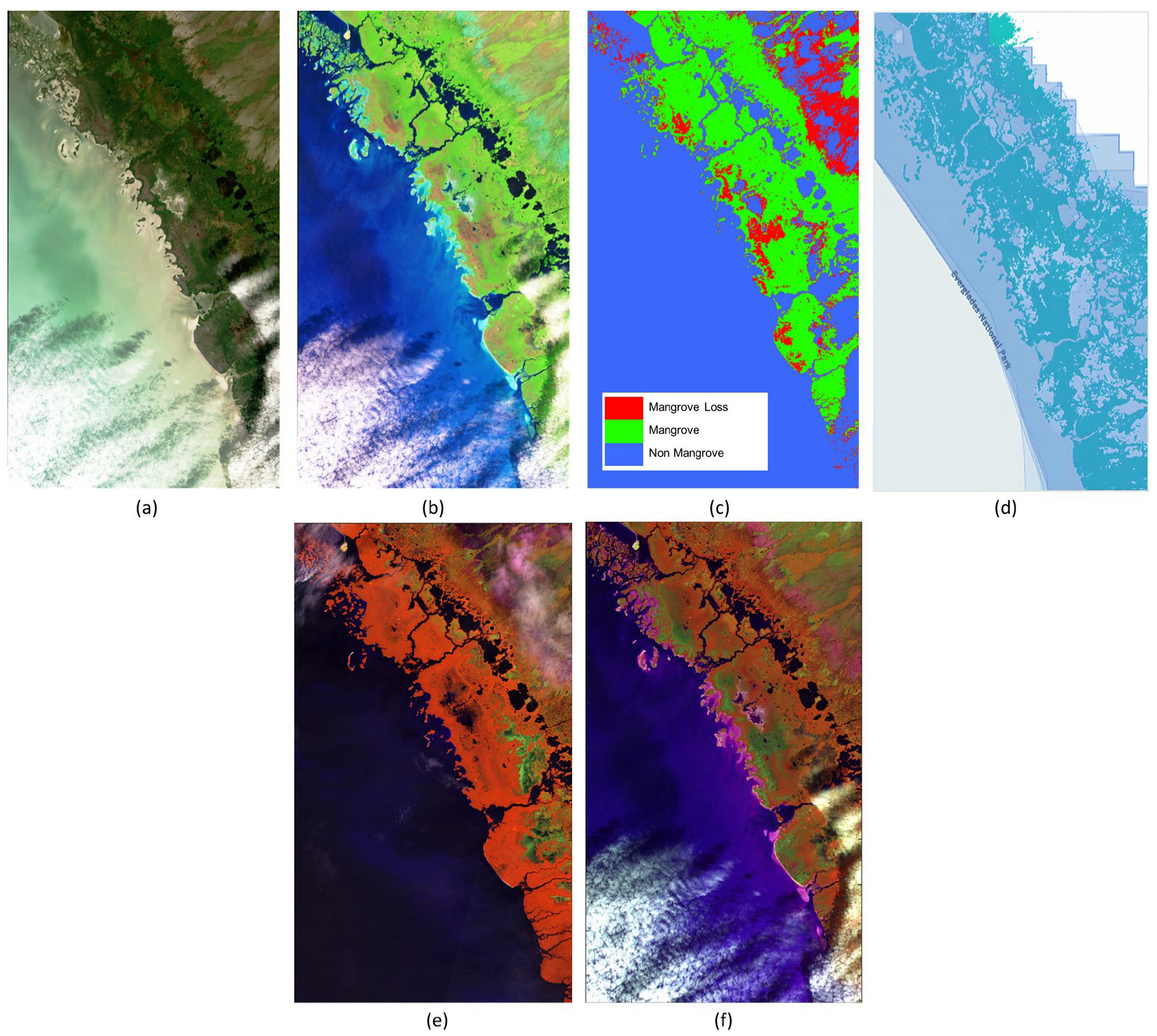
2.1. Study Area
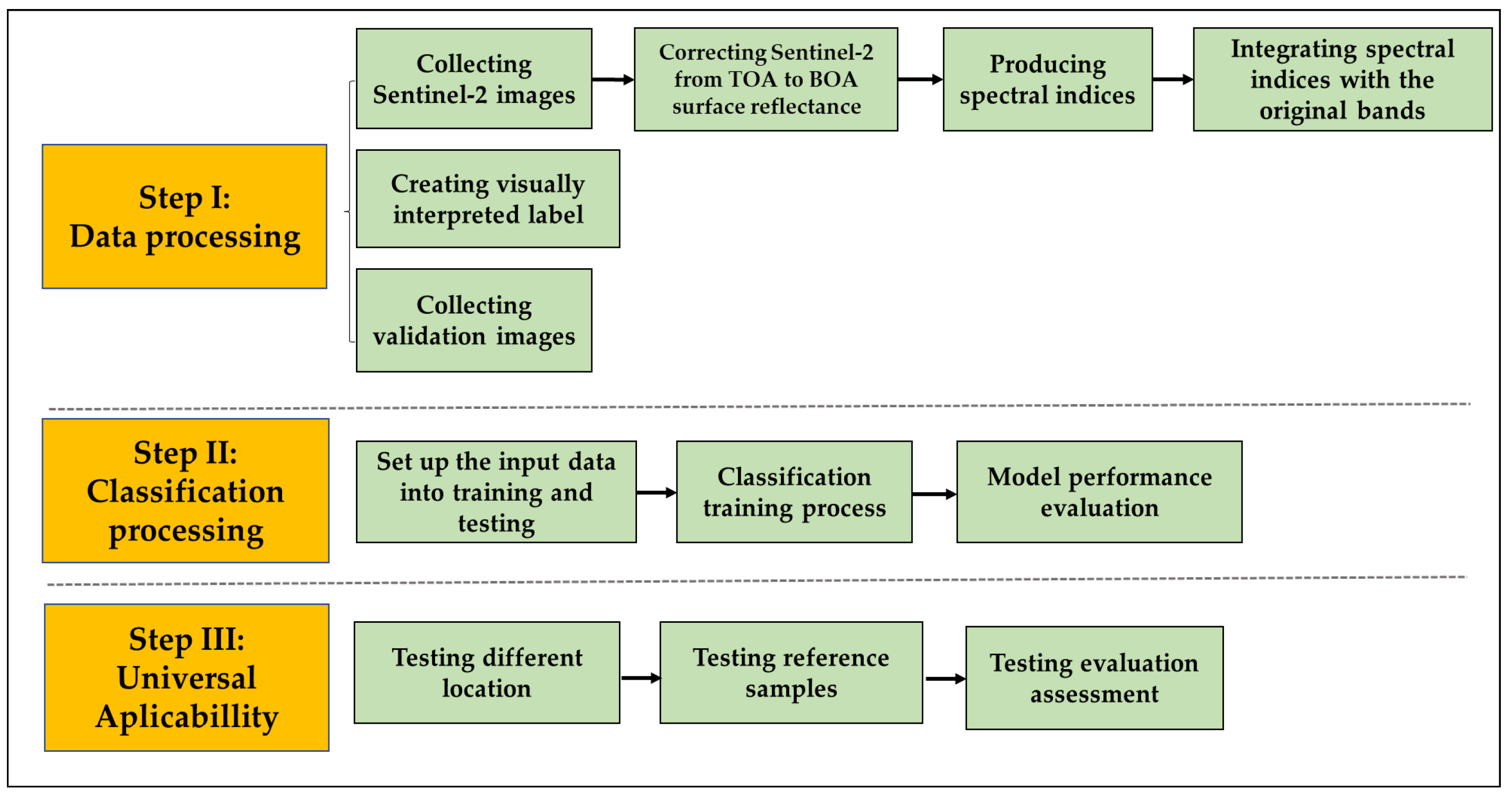
2.2. Satellite Data and Preprocessing
2.3. Input Data for Model
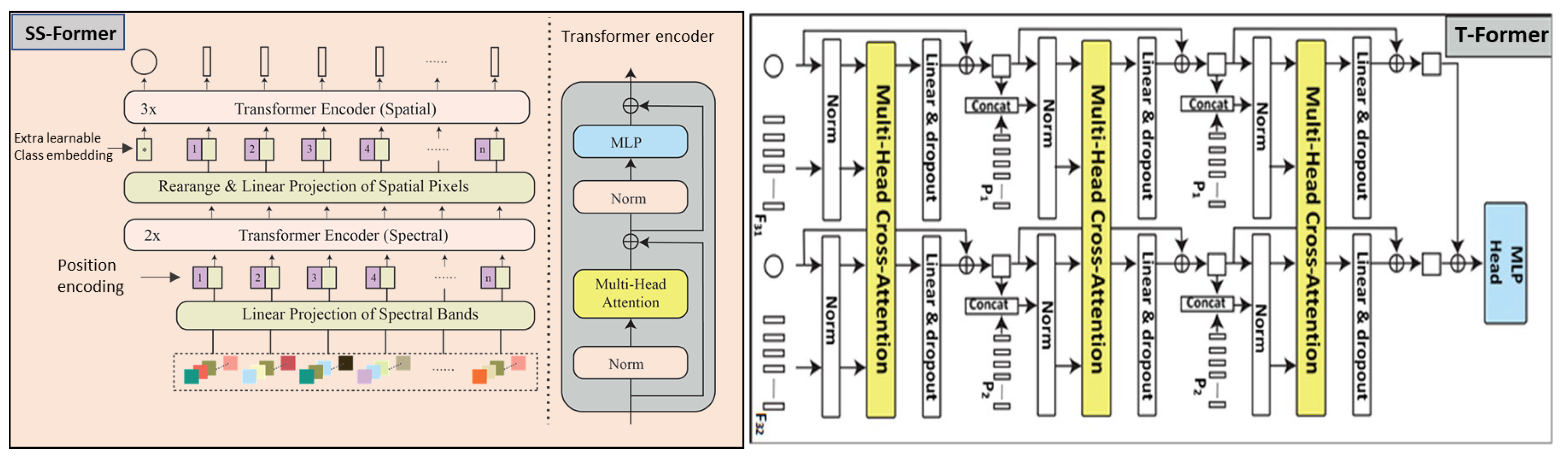
2.4. LSST-Former Architecture
2.4.1. FCN Feature Extractor
2.4.2. Transformer Classifier
2.5. Evaluation Assesment
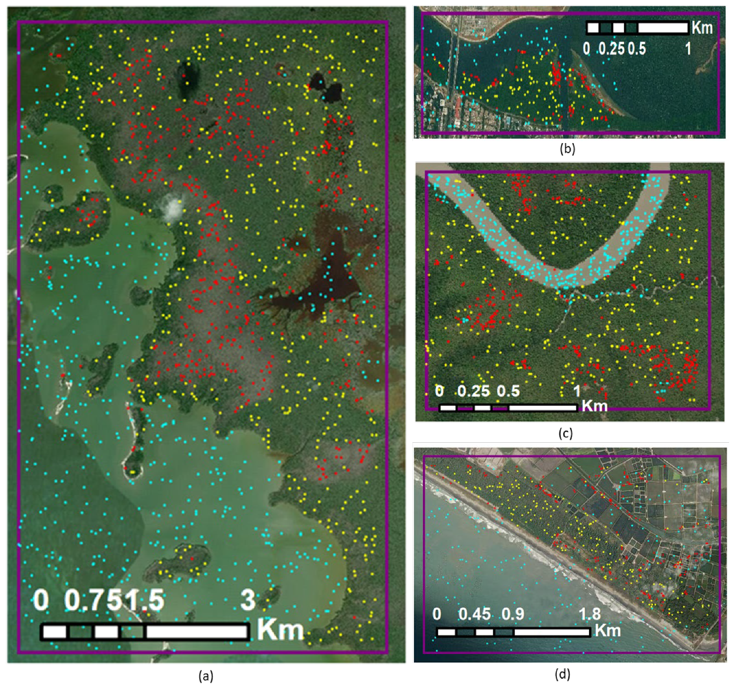
2.6. Validation of Universal Applicability Model
2.7. Implementation Detail
3. Results
3.1. LSST-Former
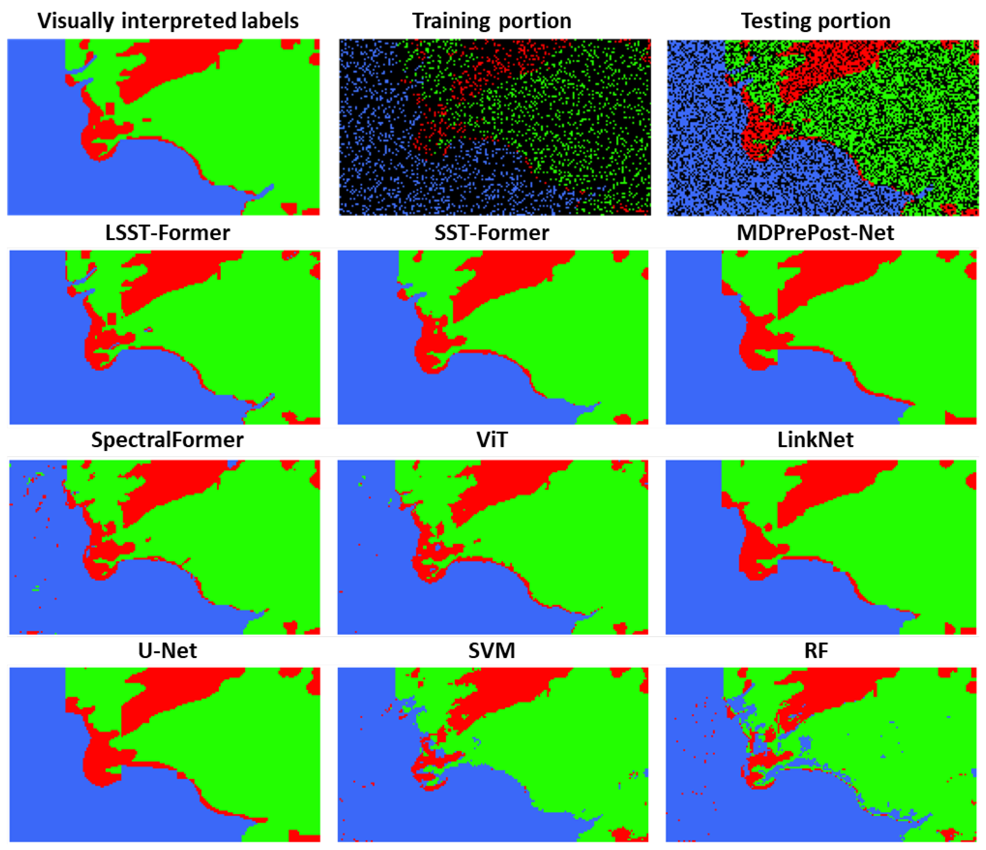
3.2. Comparison with Other Well-Established Architectures
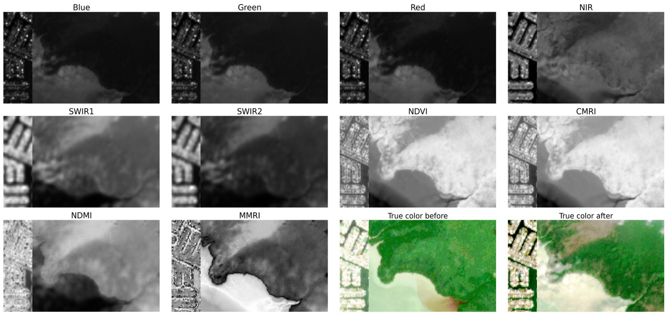
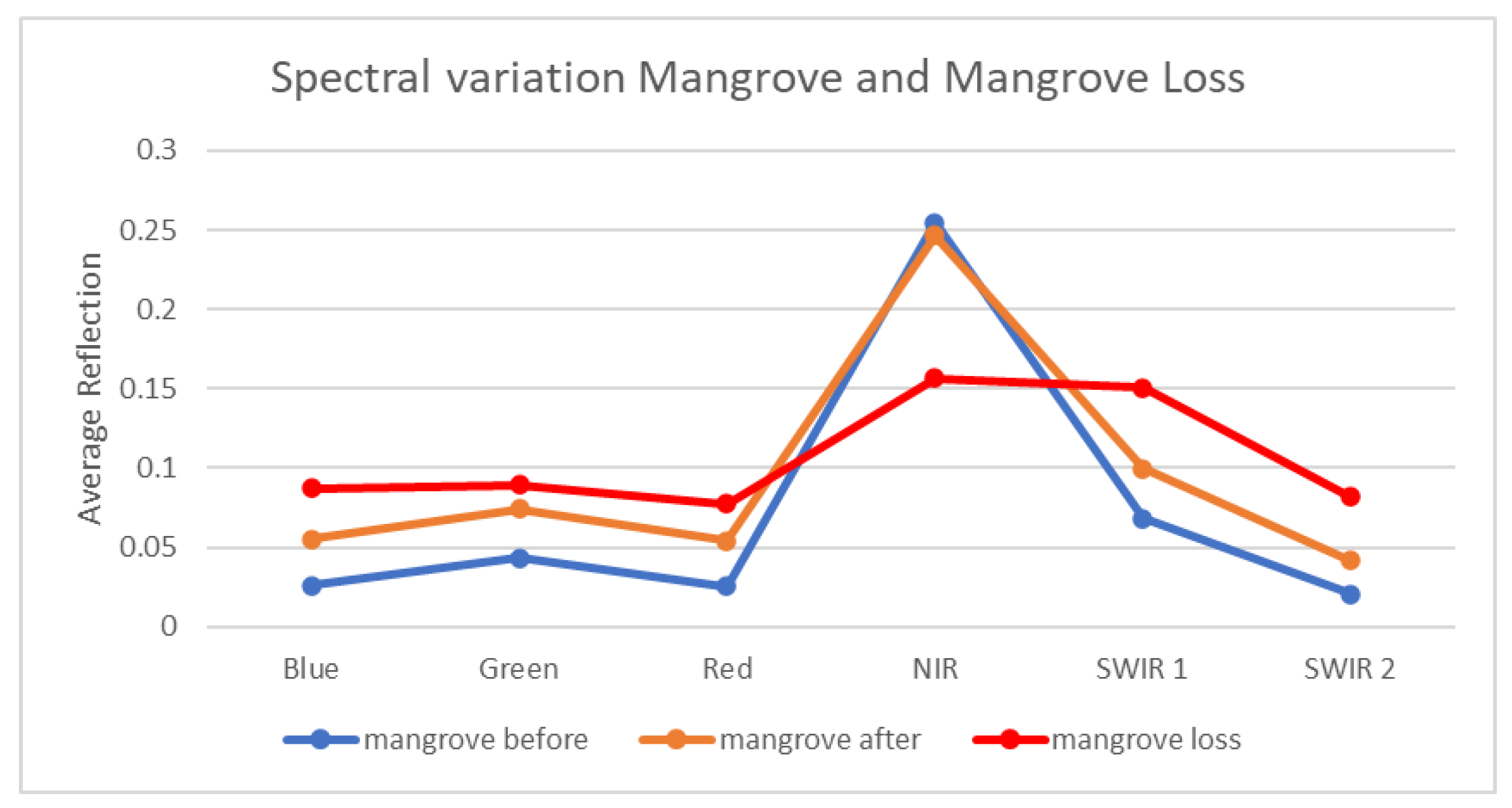
3.3. The Impact of Mangrove and Vegetation Indices
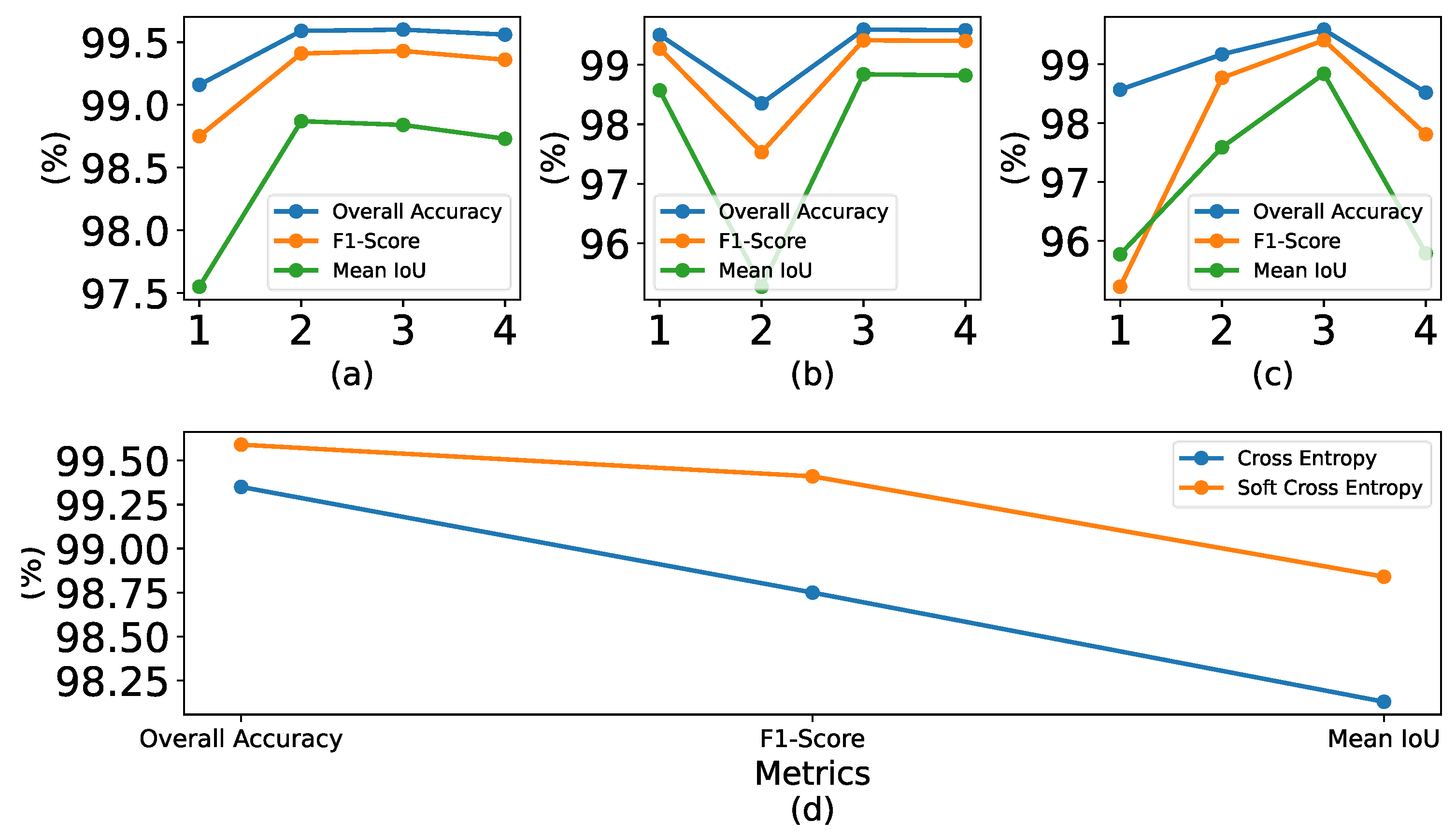
3.4. Effects of Parameters
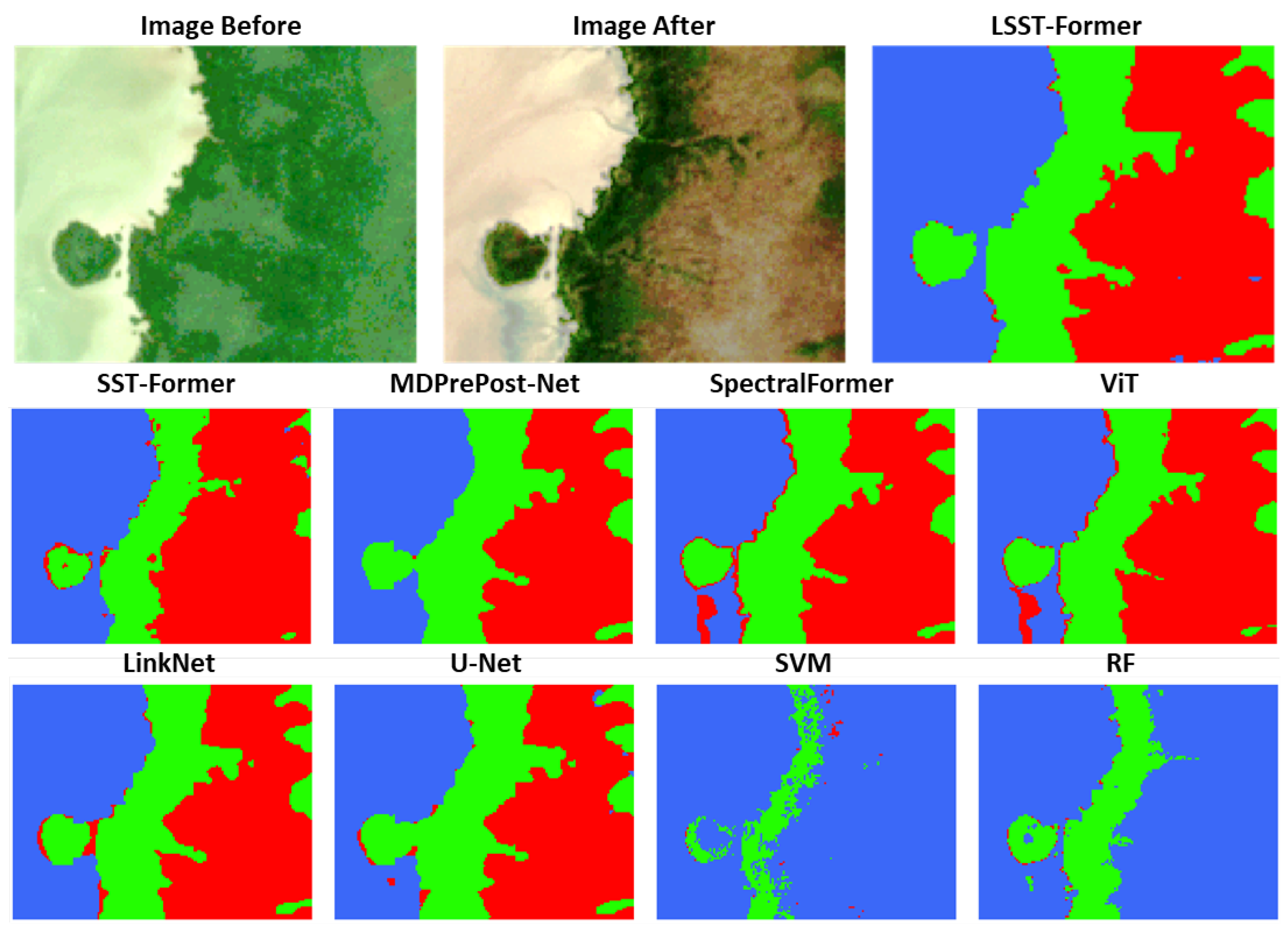
3.5. Universal Applicability of the Model
4. Discussion
5. Conclusions
Author Contributions
Funding
Data Availability Statement
Conflicts of Interest
References
- Metternicht, G.; Lucas, R.; Bunting, P.; Held, A.; Lymburner, L.; Ticehurst, C. Addressing Mangrove Protection in Australia: The Contribution of Earth Observation Technologies. In Proceedings of the IGARSS 2018—2018 IEEE International Geoscience and Remote Sensing Symposium, Valencia, Spain, 22–27 July 2018; pp. 6548–6551. [Google Scholar]
- Sidik, F.; Supriyanto, B.; Krisnawati, H.; Muttaqin, M.Z. Mangrove Conservation for Climate Change Mitigation in Indonesia. WIREs Clim. Chang. 2018, 9, e529. [Google Scholar] [CrossRef]
- Chow, J. Mangrove management for climate change adaptation and sustainable development in coastal zones. J. Sustain. For. 2018, 37, 139–156. [Google Scholar] [CrossRef]
- Islam, M.D.; Di, L.; Mia, M.R.; Sithi, M.S. Deforestation Mapping of Sundarbans Using Multi-Temporal Sentinel-2 Data & Transfer Learning. In Proceedings of the 10th International Conference on Agro-Geoinformatics (Agro-Geoinformatics) 2022, Quebec City, QC, Canada, 11–14 July 2022. [Google Scholar]
- Arifanti, V.B.; Sidik, F.; Mulyanto, B.; Susilowati, A.; Wahyuni, T.; Subarno, S.; Yulianti, Y.; Yuniarti, N.; Aminah, A.; Suita, E. Challenges and Strategies for Sustainable Mangrove Management in Indonesia: A Review. Forests 2022, 13, 695. [Google Scholar] [CrossRef]
- Wong, W.Y.; Al-Ani, A.K.I.; Hasikin, K.; Khairuddin, A.S.M.; Razak, S.A.; Hizaddin, H.F.; Mokhtar, M.I.; Azizan, M.M. Water, Soil and Air Pollutants’ Interaction on Mangrove Ecosystem and Corresponding Artificial Intelligence Techniques Used in Decision Support Systems—A Review. IEEE Access 2021, 9, 105532–105563. [Google Scholar] [CrossRef]
- Sunkur, R.; Kantamaneni, K.; Bokhoree, C.; Ravan, S. Mangroves’ Role in Supporting Ecosystem-Based Techniques to Reduce Disaster Risk and Adapt to Climate Change: A Review. J. Sea Res. 2023, 196, 102449. [Google Scholar] [CrossRef]
- Trégarot, E.; Caillaud, A.; Cornet, C.C.; Taureau, F.; Catry, T.; Cragg, S.M.; Failler, P. Mangrove Ecological Services at the Forefront of Coastal Change in the French Overseas Territories. Sci. Total Environ. 2021, 763, 143004. [Google Scholar] [CrossRef]
- Gomes, L.E.d.O.; Sanders, C.J.; Nobrega, G.N.; Vescovi, L.C.; Queiroz, H.M.; Kauffman, J.B.; Ferreira, T.O.; Bernardino, A.F. Ecosystem Carbon Losses Following a Climate-Induced Mangrove Mortality in Brazil. J. Environ. Manag. 2021, 297, 113381. [Google Scholar] [CrossRef] [PubMed]
- Ward, R.D.; Drude de Lacerda, L. Responses of mangrove ecosystems to sea level change. In Dynamic Sedimentary Environments of Mangrove Coasts; Elsevier: Amsterdam, The Netherlands, 2021; pp. 235–253. [Google Scholar]
- Vizcaya-Martínez, D.A.; Flores-de-Santiago, F.; Valderrama-Landeros, L.; Serrano, D.; Rodríguez-Sobreyra, R.; Álvarez-Sánchez, L.F.; Flores-Verdugo, F. Monitoring Detailed Mangrove Hurricane Damage and Early Recovery Using Multisource Remote Sensing Data. J. Environ. Manag. 2022, 320, 115830. [Google Scholar] [CrossRef] [PubMed]
- Kudrass, H.R.; Hanebuth, T.J.J.; Zander, A.M.; Linstädter, J.; Akther, S.H.; Shohrab, U.M. Architecture and Function of Salt-Producing Kilns from the 8th to 18th Century in the Coastal Sundarbans Mangrove Forest, Central Ganges-Brahmaputra Delta, Bangladesh. Archaeol. Res. Asia 2022, 32, 100412. [Google Scholar] [CrossRef]
- Chopade, M.R.; Mahajan, S.; Chaube, N. Assessment of land use, land cover change in the mangrove forest of Ghogha area, Gulf of Khambhat, Gujarat. Expert Syst. Appl. 2023, 212, 118839. [Google Scholar] [CrossRef]
- Quevedo, J.M.D.; Lukman, K.M.; Ulumuddin, Y.I.; Uchiyama, Y.; Kohsaka, R. Applying the DPSIR Framework to Qualitatively Assess the Globally Important Mangrove Ecosystems of Indonesia: A Review towards Evidence-Based Policymaking Approaches. Mar. Policy 2023, 147, 105354. [Google Scholar] [CrossRef]
- Gitau, P.N.; Duvail, S.; Verschuren, D. Evaluating the combined impacts of hydrological change, coastal dynamics and human activity on mangrove cover and health in the Tana River delta, Kenya. Reg. Stud. Mar. Sci. 2023, 61, 102898. [Google Scholar] [CrossRef]
- Numbere, A.O. Impact of anthropogenic activities on mangrove forest health in urban areas of the Niger Delta: Its susceptibility and sustainability. In Water, Land, and Forest Susceptibility and Sustainability; Academic Press: Cambridge, MA, USA, 2023; pp. 459–480. [Google Scholar]
- Long, C.; Dai, Z.; Zhou, X.; Mei, X.; Mai Van, C. Mapping Mangrove Forests in the Red River Delta, Vietnam. For. Ecol. Manag. 2021, 483, 118910. [Google Scholar] [CrossRef]
- Valiela, I.; Bowen, J.L.; York, J.K. Mangrove Forests: One of the World’s Threatened Major Tropical Environments. Bioscience 2001, 51, 807–815. [Google Scholar] [CrossRef]
- Goldberg, L.; Lagomasino, D.; Thomas, N.; Fatoyinbo, T. Global Declines in Human-driven Mangrove Loss. Glob. Chang. Biol. 2020, 26, 5844–5855. [Google Scholar] [CrossRef]
- Hamilton, S.E.; Casey, D. Creation of a High Spatio-Temporal Resolution Global Database of Continuous Mangrove Forest Cover for the 21st Century (CGMFC-21). Glob. Ecol. Biogeogr. 2016, 25, 729–738. [Google Scholar] [CrossRef]
- Zhang, R.; Jia, M.; Wang, Z.; Zhou, Y.; Wen, X.; Tan, Y.; Cheng, L. A comparison of Gaofen-2 and Sentinel-2 imagery for mapping mangrove forests using object-oriented analysis and random forest. IEEE J. Sel. Top. Appl. Earth Obs. Remote Sens. 2021, 14, 4185–4193. [Google Scholar] [CrossRef]
- Chen, Z.; Zhang, M.; Zhang, H.; Liu, Y. Mapping Mangrove Using a Red-Edge Mangrove Index (REMI) Based on Sentinel-2 Multispectral Images. IEEE Trans. Geosci. Remote Sens. 2023, 61, 4409511. [Google Scholar] [CrossRef]
- Zhu, Y.; Liu, K.; Liu, L.; Myint, S.W.; Wang, S.; Cao, J.; Wu, Z. Estimating and Mapping Mangrove Biomass Dynamic Change Using WorldView-2 Images and Digital Surface Models. IEEE J. Sel. Top. Appl. Earth Obs. Remote Sens. 2020, 13, 2123–2134. [Google Scholar] [CrossRef]
- Xue, Z.; Qian, S. Generalized composite mangrove index for mapping mangroves using Sentinel-2 time series data. IEEE J. Sel. Top. Appl. Earth Obs. Remote Sens. 2022, 15, 5131–5146. [Google Scholar] [CrossRef]
- Magris, R.A.; Barreto, R. Mapping and assessment of protection of mangrove habitats in Brazil. Panam. J. Aquat. Sci. 2010, 5, 546–556. [Google Scholar]
- Pham, T.D.; Yokoya, N.; Bui, D.T.; Yoshino, K.; Friess, D.A. Remote Sensing Approaches for Monitoring Mangrove Species, Structure, and Biomass: Opportunities and Challenges. Remote Sens. 2019, 11, 230. [Google Scholar] [CrossRef]
- Yu, C.; Liu, B.; Deng, S.; Li, Z.; Liu, W.; Ye, D.; Hu, J.; Peng, X. Using Medium-Resolution Remote Sensing Satellite Images to Evaluate Recent Changes and Future Development Trends of Mangrove Forests on Hainan Island, China. Forests 2023, 14, 2217. [Google Scholar] [CrossRef]
- Hu, T.; Zhang, Y.; Su, Y.; Zheng, Y.; Lin, G.; Guo, Q. Mapping the Global Mangrove Forest Aboveground Biomass Using Multisource Remote Sensing Data. Remote Sens. 2020, 12, 1690. [Google Scholar] [CrossRef]
- Zhao, C.P.; Qin, C.Z. A detailed mangrove map of China for 2019 derived from Sentinel-1 and-2 images and Google Earth images. Geosci. Date J. 2022, 9, 74–88. [Google Scholar] [CrossRef]
- Sharifi, A.; Felegari, S.; Tariq, A. Mangrove forests mapping using Sentinel-1 and Sentinel-2 satellite images. Arab. J. Geosci. 2022, 15, 1593. [Google Scholar] [CrossRef]
- Giri, C.; Pengra, B.; Long, J.; Loveland, T.R. Next Generation of Global Land Cover Characterization, Mapping, and Monitoring. Int. J. Appl. Earth Obs. Geoinf. 2013, 25, 30–37. [Google Scholar] [CrossRef]
- Rijal, S.S.; Pham, T.D.; Noer’Aulia, S.; Putera, M.I.; Saintilan, N. Mapping Mangrove Above-Ground Carbon Using Multi-Source Remote Sensing Data and Machine Learning Approach in Loh Buaya, Komodo National Park, Indonesia. Forests 2023, 14, 94. [Google Scholar] [CrossRef]
- Soltanikazemi, M.; Minaei, S.; Shafizadeh-Moghadam, H.; Mahdavian, A. Field-Scale Estimation of Sugarcane Leaf Nitrogen Content Using Vegetation Indices and Spectral Bands of Sentinel-2: Application of Random Forest and Support Vector Regression. Comput. Electron. Agric. 2022, 200, 107130. [Google Scholar] [CrossRef]
- Xu, C.; Wang, J.; Sang, Y.; Li, K.; Liu, J.; Yang, G. An Effective Deep Learning Model for Monitoring Mangroves: A Case Study of the Indus Delta. Remote Sens. 2023, 15, 2220. [Google Scholar] [CrossRef]
- Guo, Y.; Liao, J.; Shen, G. Mapping large-scale mangroves along the maritime silk road from 1990 to 2015 using a novel deep learning model and landsat data. Remote Sens. 2021, 13, 245. [Google Scholar] [CrossRef]
- Wang, Y.; Gu, L.; Jiang, T.; Gao, F. MDE-U-Net: A Multitask Deformable U-Net Combined Enhancement Network for Farmland Boundary Segmentation. IEEE Geosci. Remote Sens. Lett. 2023, 20, 3001305. [Google Scholar]
- Tran, T.L.C.; Huang, Z.C.; Tseng, K.H.; Chou, P.H. Detection of Bottle Marine Debris Using Unmanned Aerial Vehicles and Machine Learning Techniques. Drones 2022, 6, 401. [Google Scholar] [CrossRef]
- Hong, D.; Han, Z.; Yao, J.; Gao, L.; Zhang, B.; Plaza, A.; Chanussot, J. SpectralFormer: Rethinking Hyperspectral Image Classification With Transformers. IEEE Trans. Geosci. Remote Sens. 2022, 60, 5518615. [Google Scholar] [CrossRef]
- Jamaluddin, I.; Chen, Y.N.; Ridha, S.M.; Mahyatar, P.; Ayudyanti, A.G. Two Decades Mangroves Loss Monitoring Using Random Forest and Landsat Data in East Luwu, Indonesia (2000–2020). Geomatics 2022, 2, 282–296. [Google Scholar] [CrossRef]
- LeCun, Y.; Bengio, Y.; Hinton, G. Deep learning. Nature 2015, 521, 436. [Google Scholar] [CrossRef] [PubMed]
- Jamaluddin, I.; Thaipisutikul, T.; Chen, Y.N.; Chuang, C.H.; Hu, C.L. MDPrePost-Net: A Spatial-Spectral-Temporal Fully Convolutional Network for Mapping of Mangrove Degradation Affected by Hurricane Irma 2017 Using Sentinel-2 Data. Remote Sens. 2021, 13, 5042. [Google Scholar] [CrossRef]
- Lin, C.H.; Chu, M.C.; Tang, P.W. CODE-MM: Convex Deep Mangrove Mapping Algorithm Based On Optical Satellite Images. IEEE Trans. Geosci. Remote Sens. 2023, 61, 5620619. [Google Scholar] [CrossRef]
- Iovan, C.; Kulbicki, M.; Mermet, E. Deep convolutional neural network for mangrove mapping. In Proceedings of the IGARSS 2020—2020 IEEE International Geoscience and Remote Sensing Symposium, Waikoloa, HI, USA, 26 September–2 October 2020. [Google Scholar]
- Diniz, C.; Cortinhas, L.; Nerino, G.; Rodrigues, J.; Sadeck, L.; Adami, M.; Souza-Filho, P. Brazilian Mangrove Status: Three Decades of Satellite Data Analysis. Remote Sens. 2019, 11, 808. [Google Scholar] [CrossRef]
- Chen, N. Mapping mangrove in Dongzhaigang, China using Sentinel-2 imagery. J. Appl. Remote Sens. 2020, 14, 014508. [Google Scholar] [CrossRef]
- Xue, Z.; Qian, S. Two-Stream Translating LSTM Network for Mangroves Mapping Using Sentinel-2 Multivariate Time Series. IEEE Trans. Geosci. Remote Sens. 2023, 61, 4401416. [Google Scholar] [CrossRef]
- Al Dogom, D.W.; Samour, B.M.M.; Al Shamsi, M.; Almansoori, S.; Aburaed, N.; Zitouni, M.S. Machine Learning for Spatiotemporal Mapping and Monitoring of Mangroves and Shoreline Changes Along a Coastal Arid Region. In Proceedings of the IGARSS 2023—2023 IEEE International Geoscience and Remote Sensing Symposium, Pasadena, CA, USA, 16–21 July 2023. [Google Scholar]
- Li, L.; Zhang, W.; Zhang, X.; Emam, M.; Jing, W. Semi-Supervised Remote Sensing Image Semantic Segmentation Method Based on Deep Learning. Electronics 2023, 12, 348. [Google Scholar] [CrossRef]
- Wan, Q.; Ji, H.; Shen, L. Self-attention based text knowledge mining for text detection. In Proceedings of the IEEE/CVF Conference on Computer Vision and Pattern Recognition (CVPR), Seattle, WA, USA, 14–19 June 2020; pp. 5979–5988. [Google Scholar]
- Carion, N.; Massa, F.; Synnaeve, G.; Usunier, N.; Kirillov, A.; Zagoruyko, S. End-to-End Object Detection with Transformers. In Proceedings of the Computer Vision—ECCV 2020, Glasgow, UK, 23–28 August 2020; pp. 213–229. [Google Scholar]
- Dosovitskiy, A.; Beyer, L.; Kolesnikov, A.; Weissenborn, D.; Zhai, X.; Unterthiner, T.; Dehghani, M.; Minderer, M.; Heigold, G.; Gelly, S.; et al. An image is worth 16 × 16 words: Transformers for image recognition at scale. arXiv 2020, arXiv:2010.11929. [Google Scholar]
- Sun, L.; Zhao, G.; Zheng, Y.; Wu, Z. Spectral–Spatial Feature Tokenization Transformer for Hyperspectral Image Classification. IEEE Trans. Geosci. Remote Sens. 2022, 60, 5522214. [Google Scholar] [CrossRef]
- Wang, Y.; Hong, D.; Sha, J.; Gao, L.; Liu, L.; Zhang, Y.; Rong, X. Spectral–Spatial–Temporal Transformers for Hyperspectral Image Change Detection. IEEE Trans. Geosci. Remote Sens. 2022, 60, 5536814. [Google Scholar] [CrossRef]
- Liu, Y.; Hu, J.; Kang, X.; Luo, J.; Fan, S. Interactformer: Interactive Transformer and CNN for Hyperspectral Image Super-Resolution. IEEE Trans. Geosci. Remote Sens. 2022, 60, 5531715. [Google Scholar] [CrossRef]
- Shelhamer, E.; Long, J.; Darrell, T. Fully Convolutional Networks for Semantic Segmentation. IEEE Trans. Pattern Anal. Mach. Intell. 2017, 39, 640–651. [Google Scholar] [CrossRef] [PubMed]
- Ronneberger, O.; Fischer, P.; Brox, T. U-Net: Convolutional Networks for Biomedical Image Segmentation. In Proceedings of the Medical Image Computing and Computer-Assisted Intervention–MICCAI 2015, Munich, Germany, 5–9 October 2015; pp. 234–241. [Google Scholar]
- Chaurasia, A.; Culurciello, E. LinkNet: Exploiting Encoder Representations for Efficient Semantic Segmentation. In Proceedings of the 2017 IEEE Visual Communications and Image Processing (VCIP), St. Petersburg, FL, USA, 10–13 December 2017. [Google Scholar]
- Saferbekov, S.; Iglovikov, V.; Buslaev, A.; Shvets, A. Feature Pyramid Network for Multi-Class Land Segmentation. Comput. Vis. Pattern Recognit. 2018, 2, 272–2723. [Google Scholar]
- Zhao, H.; Shi, J.; Qi, X.; Wang, X.; Jia, J. Pyramid Scene Parsing Network. In Proceedings of the 2017 IEEE Conference on Computer Vision and Pattern Recognition (CVPR), Honolulu, HI, USA, 21–26 July 2017. [Google Scholar]
- Ren, M.; Triantafillou, E.; Ravi, S.; Snell, J.; Swersky, K.; Tenenbaum, J.; Larochelle, H.; Zemel, R. Meta-Learning for Semi-Supervised Few-Shot Classification. arXiv 2018, arXiv:1803.00676. [Google Scholar]
- Liu, B.; Gao, K.; Yu, A.; Ding, L.; Qiu, C.; Li, J. ES2FL: Ensemble Self-Supervised Feature Learning for Small Sample Classification of Hyperspectral Images. Remote Sens. 2022, 14, 4236. [Google Scholar] [CrossRef]
- Hamilton, S.E.; Friess, D.A. Global Carbon Stocks and Potential Emissions Due to Mangrove Deforestation from 2000 to 2012. Nat. Clim. Chang. 2018, 8, 240–244. [Google Scholar] [CrossRef]
- Rumondang, A.L.; Kusmana, C.; Budi, S.W. Species Composition and Structure of Angke Kapuk Mangrove Protected Forest, Jakarta, Indonesia. Biodiversitas J. Biol. Divers. 2021, 22, 9. [Google Scholar] [CrossRef]
- Liu, C.C.; Hsu, T.W.; Wen, H.L.; Wang, K.H. Mapping Pure Mangrove Patches in Small Corridors and Sandbanks Using Airborne Hyperspectral Imagery. Remote Sens. 2019, 11, 592. [Google Scholar] [CrossRef]
- Google Earth Engine. 2023. Available online: https://developers.google.com/earth-engine/datasets/catalog/sentinel-2 (accessed on 4 November 2023).
- Yin, F.; Lewis, P.E.; Gómez-Dans, J.L. Bayesian Atmospheric Correction over Land: Sentinel-2/MSI and Landsat 8/OLI. 2022. Available online: https://gmd.copernicus.org/articles/15/7933/2022/ (accessed on 11 March 2024).
- Shi, T.; Liu, J.; Hu, Z.; Liu, H.; Wang, J.; Wu, G. New spectral metrics for mangrove forest identification. Remote Sens. Lett. 2016, 7, 885–894. [Google Scholar] [CrossRef]
- Gupta, K.; Mukhopadhyay, A.; Giri, S.; Chanda, A.; Datta Majumdar, S.; Samanta, S.; Mitra, D.; Samal, R.N.; Pattnaik, A.K.; Hazra, S. An index for discrimination of mangroves from non-mangroves using LANDSAT 8 OLI imagery. MethodsX 2018, 5, 1129–1139. [Google Scholar] [CrossRef]
- Tucker, C.J. Red and photographic infrared linear combinations for monitoring vegetation. Remote Sens. Environ. 1979, 8, 127–150. [Google Scholar] [CrossRef]
- McFeeters, S.K. The use of the Normalized Difference Water Index (NDWI) in the delineation of open water features. Int. J. Remote Sens. 1996, 17, 1425–1432. [Google Scholar] [CrossRef]
- Xu, H. Modification of normalised difference water index (NDWI) to enhance open water features in remotely sensed imagery. Int. J. Remote Sens. 2006, 27, 3025–3033. [Google Scholar] [CrossRef]
- Nanduri, A.; Chellappa, R. Semi-Supervised Cross-Spectral Face Recognition With Small Datasets. In Proceedings of the IEEE/CVF Winter Conference on Applications of Computer Vision, Waikoloa, HI, USA, 4–8 January 2024. [Google Scholar]
- Szegedy, C.; Vanhoucke, V.; Ioffe, S.; Shlens, J.; Wojna, Z. Rethinking the Inception Architecture for Computer Vision. In Proceedings of the 2016 IEEE Conference on Computer Vision and Pattern Recognition (CVPR), Las Vegas, NV, USA, 26 June–1 July 2016. [Google Scholar]
- Vaswani, A.; Shazeer, N.; Parmar, N.; Uszkoreit, J.; Jones, L.; Gomez, A.N.; Kaiser, Ł.; Polosukhin, I. Attention is all you need. In Proceedings of the Advances in Neural Information Processing Systems, Long Beach, CA, USA, 4–9 December 2017. [Google Scholar]
- Gehring, J.; Auli, M.; Grangier, D.; Yarats, D.; Dauphin, Y.N. Convolutional sequence to sequence learning. In Proceedings of the International Conference on Machine Learning, Sydney, Australia, 6–11 August 2017; pp. 1243–1252. [Google Scholar]
- Rezatofighi, S.H.; Tsoi, N.; Gwak, J.; Sadeghian, A.; Reid, I.D.; Savarese, S. Generalized Intersection over Union: A Metric and A Loss for Bounding Box Regression. In Proceedings of the IEEE/CVF Conference on Computer Vision and Pattern Recognition, Long Beach, CA, USA, 15–20 June 2019. [Google Scholar]
- Sokolova, M.; Japkowicz, N.; Szpakowicz, S. Beyond Accuracy, F-Score and ROC: A Family of Discriminant Measures for Performance Evaluation. AI 2006 Adv. Artif. Intell. 2006, 4304, 1015–1021. [Google Scholar]
- ESRI|World Imagery Wayback. 2023. Available online: https://livingatlas.arcgis.com/wayback/ (accessed on 8 December 2023).
- Reflected Near-Infrared Waves. Available online: https://science.nasa.gov/ems/08_nearinfraredwaves/ (accessed on 9 February 2024).


| Band | Band Name | Central Wavelength (nm) | Spatial Resolution |
|---|---|---|---|
| B1 | Aerosol | 442.3 | 60 |
| B2 | Blue | 492.1 | 10 |
| B3 | Green | 559 | 10 |
| B4 | Red | 665 | 10 |
| B5 | Red Edge 1 | 703.8 | 20 |
| B6 | Red Edge 2 | 739.1 | 20 |
| B7 | Red Edge 3 | 779.7 | 20 |
| B8 | Near-infrared (NIR) | 833 | 10 |
| B8A | Red Edge 4 | 864 | 20 |
| B9 | Water-vapor | 943.2 | 60 |
| B10 | Cirrus | 1376.9 | 60 |
| B11 | Short-wave infrared (SWIR 1) | 1610.4 | 20 |
| B12 | Short-wave infrared (SWIR 2) | 2185.7 | 20 |
| Name (Scene Code) | (Lon)° | (Lat)° | Date Before | Date After | Image Size | Usage |
|---|---|---|---|---|---|---|
| Southwest Florida-1 (T17RMJ) | −81.263197 −81.2488207 | 25.6407337 25.6497094 | 20161001 | 20180104 | 145 × 100 | Training/testing |
| Southwest Florida-2 (T17RMJ) | −81.7059548 −81.7026501 | 25.9303954 25.9393493 | 20161001 | 20180104 | 35 × 100 | Training/testing |
| Southwest Florida-3 (T17RMJ) | −81.2741405 −81.2583906 | 25.6556281 25.6668073 | 20161001 | 20180104 | 159 × 125 |
Model applicability |
| Southwest Florida-4 (T17RMJ) | −81.286543 −81.2405811 | 25.6903579 25.6195264 | 20161001 | 20180104 | 464 × 786 |
Universal applicability |
| Southwest Florida-5 (T17RMJ) | −81.4133421 −81.413342 | 25.3594457 25.8375025 | 20161001 | 20180104 | 3000 × 5276 |
Universal applicability |
| PIK Jakarta (T48MXU) | 106.7384884 106.7644093 | −6.1047809 −6.0976117 | 20190505 | 20191101 | 289 × 81 |
Universal applicability |
| Papua (T54LVR) | 140.2627755 140.2871514 | −8.3748976 −8.3514604 | 20171104 | 20181005 | 270 × 260 |
Universal applicability |
| Tainan (T50QRL) | 120.079663 120.1093595 | 23.0201424 23.0383102 | 20180302 | 20180903 | 310 × 209 |
Universal applicability |
| Total Label (Pixel) | Formula | Reference |
|---|---|---|
| NDVI | (NIR − Red)/(NIR + Red) | [69] |
| NDWI | (Green − NIR)/(Green + NIR) | [70] |
| CMRI | (NDVI − NDWI) | [68] |
| NDMI | (SWIR2 − Green)/(SWIR2 + Green) | [67] |
| MNDWI | (Green − SWIR1)/(Green + SWIR2) | [71] |
| MMRI | (|MNDWI| − |NDVI|)/(|MNDWI + |NDVI|) | [44] |
| Total Label (Pixels) | Training (Pixels) | Testing (Pixels) |
|---|---|---|
| Non-mangrove | 1194 | 4549 |
| Mangrove | 1268 | 4608 |
| Mangrove loss | 408 | 1560 |
| Total | 2870 | 10,717 |
| Metrics | Non-Mangrove | Intact Mangrove | Mangrove Loss |
|---|---|---|---|
| IoU | 99.62 | 99.33 | 97.59 |
| F1-Score | 99.81 | 99.66 | 98.78 |
| Precision | 99.91 | 99.58 | 98.72 |
| Recall | 99.71 | 99.74 | 98.84 |
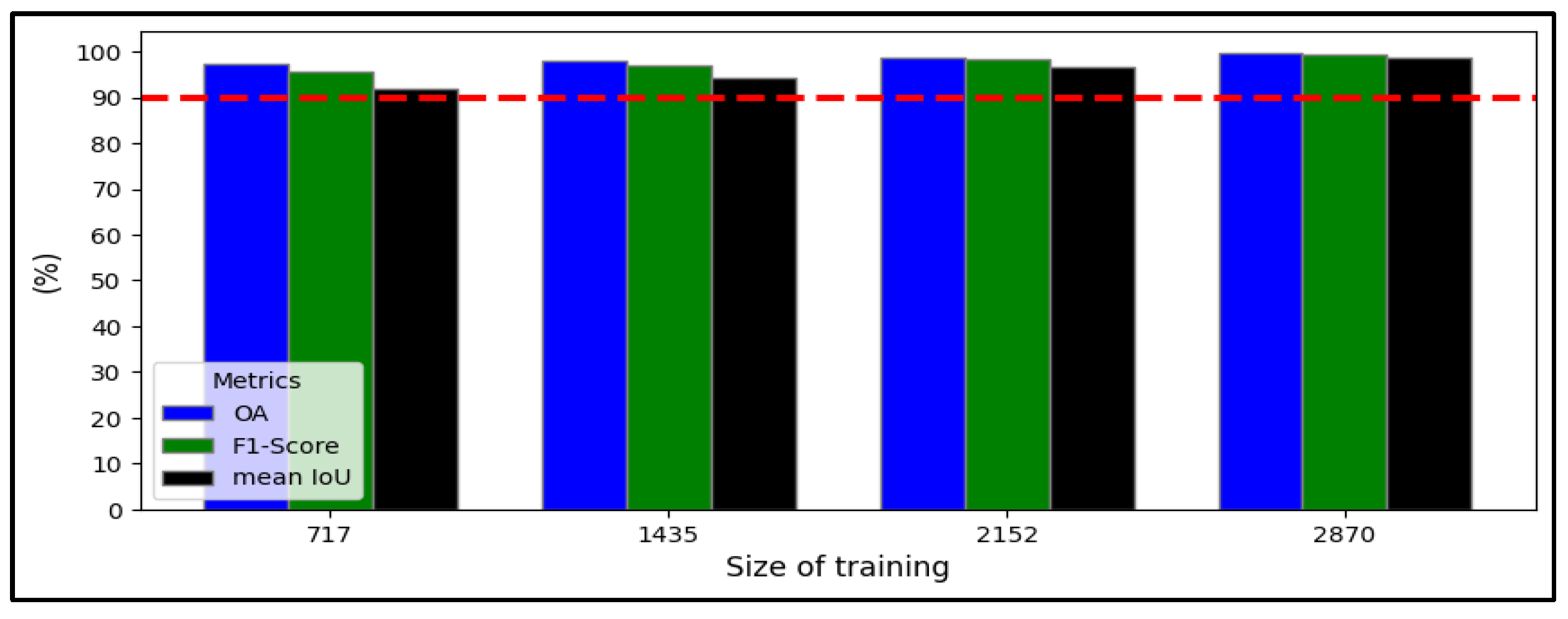
| Training Size | Overall Accuracy | F1-Score | Mean IoU |
|---|---|---|---|
| 717 | 97.18 | 95.74 | 92.05 |
| 1435 | 98.02 | 97.02 | 94.34 |
| 2152 | 98.81 | 98.21 | 96.54 |
| 2870 | 99.59 | 99.41 | 98.84 |
| Architecture | Overall Accuracy | F1-Score | Mean IoU |
|---|---|---|---|
| LSST-Former | 99.59 | 99.41 | 98.84 |
| No LinkNet | 97.58 | 96.34 | 93.10 |
| No SST-Former | 95.81 | 91.03 | 84.55 |
| Class | Non-Temporal Imagery | Temporal Imagery | |||||||
|---|---|---|---|---|---|---|---|---|---|
| Conventional Network | Convolution Network | Transformer Network | Convolution Network | Transformer Network | |||||
| RF | SVM | U-Net | LinkNet | Vit | Spectralformer | MDPrePost-Net | SST-Former | LSST-Former | |
| IoU Non-Mg | 81.33 | 88.33 | 92.41 | 92.42 | 96.04 | 95.71 | 93.06 | 98.39 | 99.62 |
| IoU MgLs | 55.60 | 57.40 | 54.80 | 65.79 | 76.69 | 82.29 | 67.44 | 85.33 | 97.59 |
| IoU Mg | 90.27 | 94.37 | 93.57 | 95.44 | 94.58 | 96.32 | 94.56 | 95.58 | 99.33 |
| Mean IoU | 75.74 | 80.04 | 80.26 | 84.55 | 89.10 | 91.44 | 85.02 | 93.10 | 98.84 |
| F1-Score | 85.35 | 87.94 | 87.84 | 91.03 | 86.81 | 95.41 | 91.39 | 96.34 | 99.41 |
| OA | 90.84 | 93.64 | 94.42 | 95.81 | 96.20 | 96.96 | 95.71 | 97.58 | 99.59 |
| Architecture | Overall Accuracy | F1-Score | Mean IoU |
|---|---|---|---|
| RGB | 94.31 | 92.01 | 85.72 |
| RGB NIR | 94.70 | 91.10 | 86.71 |
| RGB NIR SWIR1 SWIR2 | 95.03 | 93.13 | 87.53 |
| All | 99.59 | 99.41 | 98.84 |
| Prediction | Reference Data | |||
| NonMg | Mg | MgLs | ||
| NonMg | 493 | 2 | 5 | |
| Mg | 1 | 492 | 7 | |
| MgLs | 3 | 12 | 485 | |
| Prediction | Reference Data | |||
| NonMg | Mg | MgLs | ||
| NonMg | 97 | 3 | 0 | |
| Mg | 0 | 98 | 2 | |
| MgLs | 2 | 10 | 88 | |
| Prediction | Reference Data | |||
| NonMg | Mg | MgLs | ||
| NonMg | 281 | 12 | 7 | |
| Mg | 1 | 294 | 5 | |
| MgLs | 5 | 28 | 267 | |
| Prediction | Reference Data | |||
| NonMg | Mg | MgLs | ||
| NonMg | 197 | 2 | 1 | |
| Mg | 6 | 187 | 7 | |
| MgLs | 25 | 2 | 173 | |
| NonMg | Mg | MgLs | OA | Kappa | |
|---|---|---|---|---|---|
| Southwest Florida-4 | 0.986 | 0.984 | 0.97 | 0.98 | 0.97 |
| PIK Jakarta, Indonesia | 0.97 | 0.98 | 0.88 | 0.9433 | 0.9150 |
| Papua, Indonesia | 0.937 | 0.98 | 0.89 | 0.9356 | 0.9033 |
| Tainan, Taiwan | 0.985 | 0.935 | 0.865 | 0.9283 | 0.8925 |
Disclaimer/Publisher’s Note: The statements, opinions and data contained in all publications are solely those of the individual author(s) and contributor(s) and not of MDPI and/or the editor(s). MDPI and/or the editor(s) disclaim responsibility for any injury to people or property resulting from any ideas, methods, instructions or products referred to in the content. |
© 2024 by the authors. Licensee MDPI, Basel, Switzerland. This article is an open access article distributed under the terms and conditions of the Creative Commons Attribution (CC BY) license (https://creativecommons.org/licenses/by/4.0/).
Share and Cite
Panuntun, I.A.; Jamaluddin, I.; Chen, Y.-N.; Lai, S.-N.; Fan, K.-C. LinkNet-Spectral-Spatial-Temporal Transformer Based on Few-Shot Learning for Mangrove Loss Detection with Small Dataset. Remote Sens. 2024, 16, 1078. https://doi.org/10.3390/rs16061078
Panuntun IA, Jamaluddin I, Chen Y-N, Lai S-N, Fan K-C. LinkNet-Spectral-Spatial-Temporal Transformer Based on Few-Shot Learning for Mangrove Loss Detection with Small Dataset. Remote Sensing. 2024; 16(6):1078. https://doi.org/10.3390/rs16061078
Chicago/Turabian StylePanuntun, Ilham Adi, Ilham Jamaluddin, Ying-Nong Chen, Shiou-Nu Lai, and Kuo-Chin Fan. 2024. "LinkNet-Spectral-Spatial-Temporal Transformer Based on Few-Shot Learning for Mangrove Loss Detection with Small Dataset" Remote Sensing 16, no. 6: 1078. https://doi.org/10.3390/rs16061078
APA StylePanuntun, I. A., Jamaluddin, I., Chen, Y.-N., Lai, S.-N., & Fan, K.-C. (2024). LinkNet-Spectral-Spatial-Temporal Transformer Based on Few-Shot Learning for Mangrove Loss Detection with Small Dataset. Remote Sensing, 16(6), 1078. https://doi.org/10.3390/rs16061078