Article

Forest Aboveground Biomass Estimation Using Multisource Remote Sensing Data and Deep Learning Algorithms: A Case Study over Hangzhou Area in China

1
Department of Intelligent Transportation and Spatial Informatics, School of Transportation, Southeast University, Nanjing 211102, China
2
Key Laboratory of Safety and Risk Management on Transport Infrastructures, Ministry of Transport, PRC, Nanjing 210000, China
3
College of Geography and Tourism, Hengyang Normal University, Hengyang 421002, China
4
School of Geospatial Engineering and Science, Sun Yat-sen University, Guangzhou 510275, China
*
Author to whom correspondence should be addressed.
Remote Sens. 2024, 16(6), 1074; https://doi.org/10.3390/rs16061074
Submission received: 4 January 2024 / Revised: 28 February 2024 / Accepted: 14 March 2024 / Published: 19 March 2024
(This article belongs to the Special Issue SAR in Big Data Era III)

Abstract

:
The accurate estimation of forest aboveground biomass is of great significance for forest management and carbon balance monitoring. Remote sensing instruments have been widely applied in forest parameters inversion with wide coverage and high spatiotemporal resolution. In this paper, the capability of different remote-sensed imagery was investigated, including multispectral images (GaoFen-6, Sentinel-2 and Landsat-8) and various SAR (Synthetic Aperture Radar) data (GaoFen-3, Sentinel-1, ALOS-2), in aboveground forest biomass estimation. In particular, based on the forest inventory data of Hangzhou in China, the Random Forest (RF), Convolutional Neural Network (CNN) and Convolutional Neural Networks Long Short-Term Memory Networks (CNN-LSTM) algorithms were deployed to construct the forest biomass estimation models, respectively. The estimate accuracies were evaluated under the different configurations of images and methods. The results show that for the SAR data, ALOS-2 has a higher biomass estimation accuracy than the GaoFen-3 and Sentinel-1. Moreover, the GaoFen-6 data is slightly worse than Sentinel-2 and Landsat-8 optical data in biomass estimation. In contrast with the single source, integrating multisource data can effectively enhance accuracy, with improvements ranging from 5% to 10%. The CNN-LSTM generally performs better than CNN and RF, regardless of the data used. The combination of CNN-LSTM and multisource data provided the best results in this case and can achieve the maximum R2 value of up to 0.74. It was found that the majority of the biomass values in the study area in 2018 ranged from 60 to 90 Mg/ha, with an average value of 64.20 Mg/ha.

1. Introduction

Zhejiang Province, China, with a 61.15% forest cover, ranks among China’s top five highest percentages of forested areas. The subtropical monsoon climate over this region leads to rich forest resources [1]. As the mainstay of terrestrial ecosystems, forests regulate the regional ecological environment and play a crucial role in maintaining the Earth’s carbon balance, with their carbon sequestration capacity accounting for 76–98% of that of global vegetation. Any changes in the carbon stocks of forests could cause changes in global atmospheric CO2 concentrations. A rapid, accurate and macroscopic understanding of the spatial distribution of forest resources, biomass and carbon stock values is important for supporting efforts to balance the Earth’s carbon cycle, purify the ecosystem and reduce the rate of global warming [2].
As a key measure of forest carbon stocks, forest biomass is a prominent measure of the carbon sequestration capacity of forests and the basis for assessing the regional forest carbon balance [3]. The use of field measurements is one of the most effective methods to measure forest biomass with in situ data and anisotropic growth equation. It is more accurate to combine this data with multiple inventory results for better modeling [4]. However, the high cost and low coverage of this method limit its application on regional and global scales. Remote sensing instruments are regarded as a good compensation as they can provide consistent data sources with high frequency and global coverage at the multiscale. In particular, extensive overviews have demonstrated the value of using optical and SAR sensors to assess the damage to forests and to investigate the distribution, structure and dynamics of forest resources [5,6]. The spectral information in relation to surface features in optical image and electromagnetic information (e.g., slope, shape and surface roughness) in SAR images suggest the combination of both datasets for forest parameter estimation, although heterogeneous data may also introduce errors [7,8].
From the technical viewpoint, multiple linear regression is commonly utilized to estimate biomass [9]. For example, Zheng et al. [10] extracted vegetation indices from ETM images and added forest age information that is highly correlated with biomass to determine the biomass threshold for each forest age category. The multiple linear regression was deployed to estimate the biomass of pine and broadleaf forests with a validated R2 value of 0.67. However, linear regression cannot represent nonlinear relationships well. Therefore, machine learning is introduced to enhance the estimation accuracy. Yue et al. [11] used RADARSAT-2 fully polarimetric SAR, GF1-WFV multispectral data and the biomass of winter wheat to construct a biomass estimation model for winter wheat using Random Forest (RF), and the results revealed that the model that combined the correlation coefficient analysis with the forest data had the higher accuracy. Zhou et al. [12] extracted 34 features from Landsat-8 imagery, together with in situ data, to build a biomass estimation model using Support Vector Machine (SVM) and evaluated the estimation accuracy of the model using 32 samples, with an R2 of 0.5858 after setting the optimal parameters. Aguirre-Salado et al. associated satellite-derived, climatic, and topographic predictor variables with national forest inventory data to map biomass along the northern border of Mexico by means of the K-Nearest Neighbor (KNN) [13]. Hong et al. [14] utilized airborne LiDAR data, ground-based monitoring and optical remote sensing techniques to investigate the Larix olgensis plantation in Heilongjiang Province and proposed a set of methods, namely rapid, universal, multiscale (single tree, stand, management unit, and region), and unit-high-precision continuous monitoring methods for forest biomass components. Singh et al. [15] proposed a framework to monitor aboveground biomass (AGB) at finer scales using open-source satellite data. The framework integrated four machine learning (ML) techniques with field surveys and satellite data. The application of this framework is exemplified in a case study of a dry deciduous tropical forest in India. The results revealed that for wet season Sentinel-2 satellite data, the Random Forest (adjusted R2 = 0.91) and Artificial Neural Network (adjusted R2 = 0.77) ML models were better suited for estimating AGB in the study area. Thus, researchers tend to apply machine learning methods that are used more frequently and with better results, such as RF and SVM. More advanced machine learning approaches (e.g., gradient boosting and convolutional neural networks (CNNs)) are still being underutilized. Subsequent studies need to increase the exploration and application of new methodologies.
From the data viewpoint, researchers typically combine multiple optical and SAR images from different sensors. Guerra-Hernández et al. [16] combined recent The Ice, Cloud, and Land Elevation Satellite-2 (ICESat-2), Sentinel-1, Sentinel-2 and ALOS2/PALSAR2 data for extrapolation of AGB estimates and AGB mapping. Nandy et al. [17] integrated ICESat-2 and Sentinel-1 data for mapping forest canopy height, and used RF methods to apply forest canopy height and Sentinel-2 derived variables to map the spatial distribution of AGB. Shendryk [18] proposed a machine learning method that fuses open access Global Ecosystem Dynamics Investigation (GEDI), Sentinel-1, Sentinel-2, elevation and land cover data for large-area AGBD mapping, and the model performs well. Currently, the important data source for many related studies is the Sentinel satellites, and researchers lack research and application of data from other satellites, such as China’s Gaofen series of satellites. Many researchers have concluded that the fusion of multisource remote sensing data can lead to a more accurate prediction of aboveground forest biomass. Can the accuracy of predictions be further improved by adding more sources of remote sensing data to the study? This is a question worth exploring.
In the past five years, few studies have demonstrated that deep learning brings a significant opportunity for predicting the forest parameters [19,20,21]. The estimation accuracy benefits significantly from the capability of deep learning to extract invariant and abstract features automatically from remote-sensed imagery. The trained learning models are also likely to be generalized to other forest scenarios with similar characteristics. However, the complexity of models and the data requirements (e.g., the availability of forest inventory data) limit the application of deep learning algorithms on biomass estimation. It is therefore important to assess the advantages and disadvantages of such algorithms on specific datasets and scenes carefully [22].
To this end, in response to the current state of data and methods, this experiment decided to use advanced machine learning methods and more diverse remote sensing data. This paper aims to explore the potential of different remote-sensed imagery and deep learning algorithms on forest aboveground biomass estimation. Particularly, various remote-sensed data, including optical data (GaoFen-6, Sentinel-2 and Landsat-8) and SAR data (GaoFen-3, Sentinel-1 and ALOS-2), together with three algorithms such as RF, the Convolutional Neural Networks (CNNs) and Long Short-Term Memory Networks (CNN-LSTMs), are used. We first select the feature variables from individual sources by maximizing the correlation between remote-sensed data and in situ data. Then, the aboveground biomass of the forest is estimated using different configurations of methods and feature variables. The best one was finally selected to map the spatial distribution of forests over the Lin’an district of Hangzhou, northwestern Zhejiang Province, China.

2. Materials and Methods

2.1. Study Area

The study area shown in Figure 1 is located in the Lin’an district of Hangzhou, in northwestern Zhejiang Province, with a longitude of 118°51′ to 119°52′ east and a latitude of 29°56′ to 30°23′ north. The area has a subtropical monsoon climate with four distinct seasons, an annual average temperature of 16.4 °C, annual precipitation of 1500.0~1628.6 mm, 1847.3 annual sunshine hours and a frost-free period of 237 days. The area has an altitude of 60~120 m, low hills, and a large area of forest coverage; the region is rich in species, and its main forest types include mixed coniferous forests and mixed broad-leaved forests, with the broad-leaved forests, with the dominant species being horsetail pine, fir, etc.

2.2. Data Collection and Processing

2.2.1. Field Data

The National Forest Resources Continuous Inventory is a forest resource survey that aims to understand the quantity, quality, and patterns of growth. It is an important part of the comprehensive monitoring of China’s forest resources. Forest resource inventory data are the most exhaustive and exact data reflecting the forest resources in China. The main survey contents include forest type, accumulation, growth, and harvesting data [23].
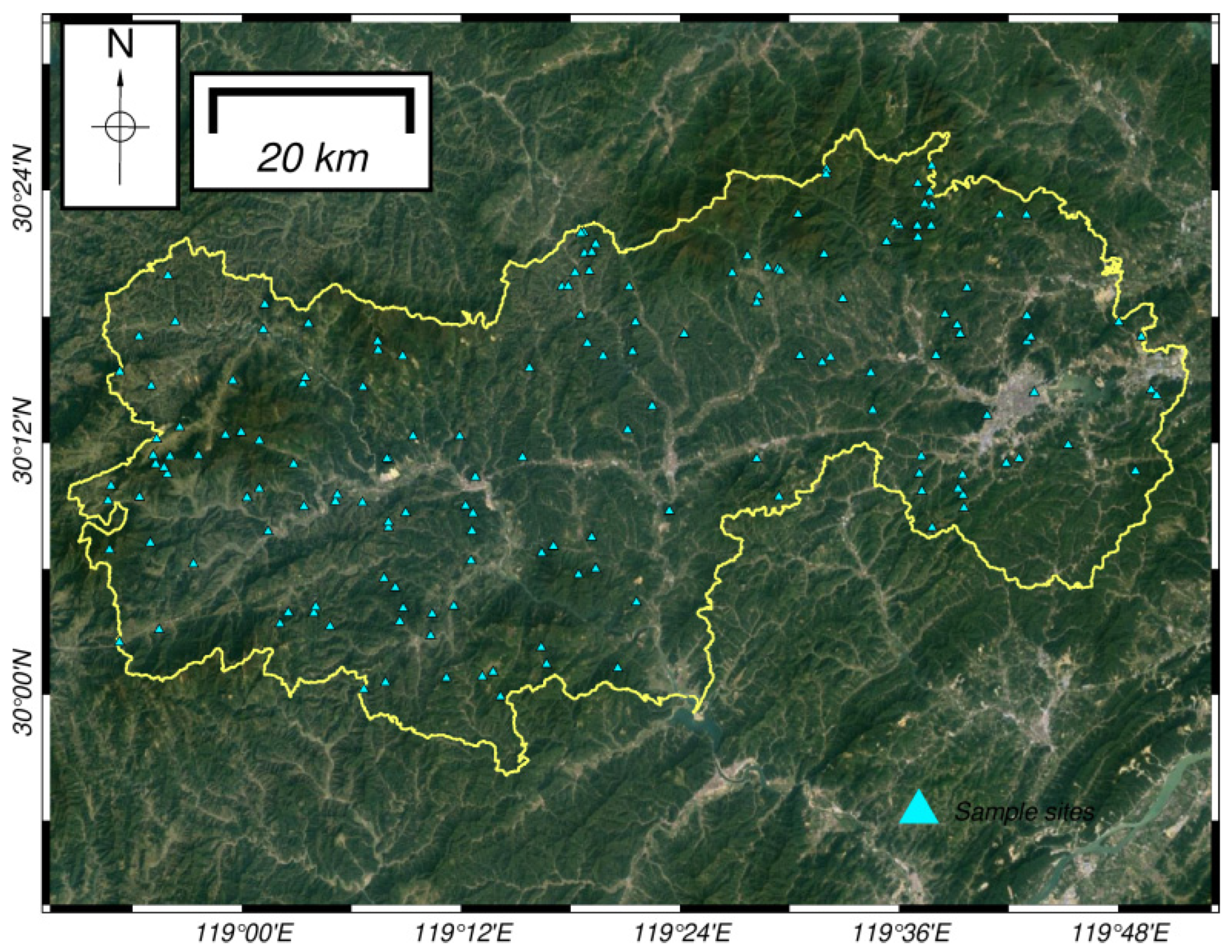
The ground data used in this study are from the ninth forest inventory in 2018, and all sample plots in the Lin’an district were plotted in Figure 2 to select those with forestland and uniform forest stands; those with agricultural land, construction land and other non-forest land types and zero storage volume were excluded [24]. The study area is rich in forest resources, and the dominant tree species in the screened sample plots mainly include four species: fir, horsetail pine, hard broad and soft broad. The data include the location, date, origin and species composition. For each sample plot, the main investigation includes diameter at breast height, tree height and species.
The aboveground data in Figure 2 is used to calculate forest aboveground biomass. In this paper, the aboveground biomass of individual standing trees was estimated by species using the growth models and parameters for each tree species or species group that have been documented (Table 1), and each dominant tree species was classified as one of four species categories, according to the species distribution of the forest: fir (Cunninghamia lanceolata (Lamb.) Hook., belonging to the Cupressaceae), horsetail pine (Pinus massoniana Lamb., belonging to the Pinaceae), hard broad and soft broad. ArcGIS was used to calculate the extremes and standard deviations at each sample site, and sample sites with high data dispersion and abnormal data were deleted. Finally, 160 sample sites were obtained, of which 130 were used for modeling, and 30 were used for testing.

2.2.2. Optical and SAR Data Processing

Successfully launched on 2 June 2018 as China’s first precise agricultural observation satellite, the Gaofen-6 (GF-6) satellite is mainly used for agriculture-related monitoring of crop growth, soil conditions observations and forestry [25]. This satellite has eight-band Complementary Metal Oxide Semiconductor (CMOS) detectors, and it is the first domestic satellite to carry the red-edge band that can effectively monitor the growth of vegetation. According to the timing and area of the ground data sampling, a GF-6 WFV image with a spatial resolution of 16 m from 5 September 2018 was acquired.
Sentinel-2 is a multispectral high-resolution imaging satellite that is primarily used to provide monitoring information for agricultural and forestry crops [26]. The Sentinel-2 wide-field, high-resolution multispectral imager (MSI) covers 13 spectral bands (443 nm-2190 nm) with a width of 290 km, encompassing the visible, near-infrared and shortwave infrared bands, with spatial resolutions of 10 m, 20 m and 60 m. Two Level-1C Sentinel-2 multispectral images acquired on 29 October and 10 November 2018 were selected.
The Landsat-8 satellite has a total of 11 bands, and the OLI Land Imager has nine bands with an imaging width of 185 km. The range of the panchromatic band has been adjusted compared to that of the Landsat-7 ETM sensor, with a narrower range to better distinguish vegetation areas from other areas. Two images covering the study area were downloaded from the USGS website, and the image information is shown in Table 2. The L1T product is the data product obtained after radiometric correction and geometric refinement using ground control points and digital elevation models.
The Gaofen-3 satellite (GF-3) launched on 10 August 2016 is the first C-band multi-polarimetric synthetic aperture radar satellite (SAR) in China with a resolution of 1 m and 12 imaging modes [27,28]. A dual-polarization data with Stripmap mode acquired on 17 November 2018 was selected according to the test site and the timing of ground data acquisition. Two dual-polarimetric Sentinel-1 images were obtained in interferometric wide (IW) imaging mode, with imaging dates of 1 October and 13 October 2018, as shown in Table 3. The L-band ALOS-2 SAR image acquired on 8 November 2018 with the Fine Beam Dual Polarization (FBD) mode was selected.
During SAR data pre-processing, radiometric terrain correction and calibration were carried out for all SAR images, followed by co-registering to the SRTM digital elevation model (DEM) and geocoding into the geographic coordinate system (EPSG: 4326) by using the ESA open-source software SNAP 9.0.0. Adaptive Lee filtering was deployed to eliminate the speckle nature in SAR images. The polarization decomposition provides a reasonable physical explanation of the scattering mechanism of the target, while the incoherent polarization target decomposition can extract the scattering characteristics of the feature more effectively according to different scattering mechanisms [29]. Because the SAR data used in this study were all in dual-polarization mode, a dual-polarization Cloude decomposition was used to extract the polarization decomposition parameters, including entropy, anisotropy and the mean scattering angle.
For multispectral images, the meridian convergence angle (angle of true north and coordinate north) was calculated for each pixel, and the UTM projection was transformed into latitude and longitude coordinates. Before analyzing the optical images, all required atmospheric corrections. ENVI (The Environment for Visualizing Images) is a complete remote sensing image processing platform with better Flaash atmospheric correction. All images were atmospherically corrected using the FLAASH tool of ENVI 5.3.

2.3. Characteristic Variable Selection

Multispectral images contain band information, vegetation indices and other physical variables [30]; SAR images provide backward scattering features, interference information and polarization decomposition features [31,32]. Several features related to aboveground biomass were extracted, including the Normalized Difference Vegetation Index (NDVI), Difference Vegetation Index (DVI), Green Normalized Difference Vegetation (GNDV), Ratio Vegetation Index (RVI) and statistics. On the other hand, texture information and polarization decomposition features in SAR images were also extracted. The details of the feature are shown in Table 4, Table 5 and Table 6.

2.4. Experimental Models

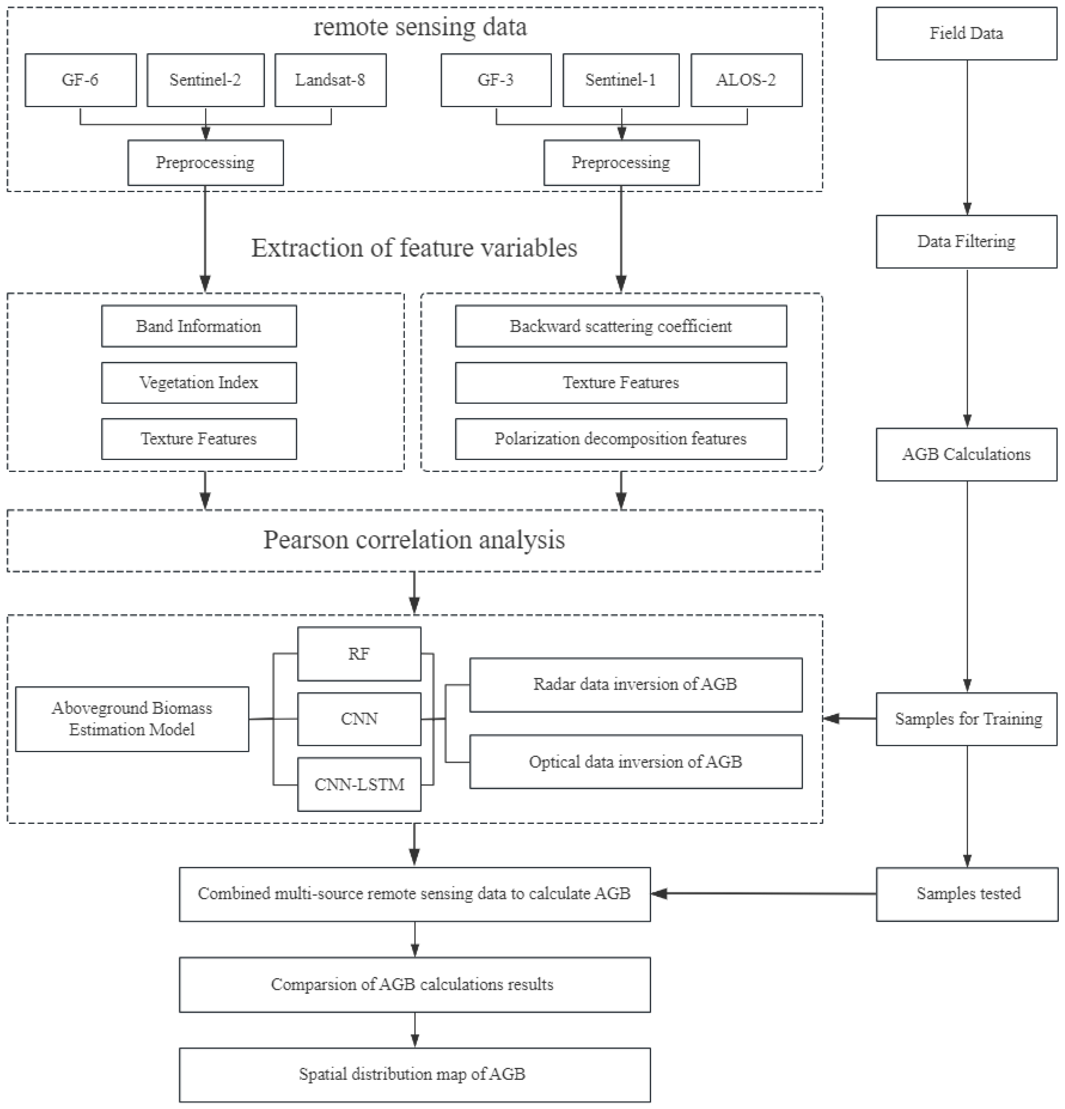
The flowchart of the research for this article is shown in Figure 3.

2.4.1. Random Forest

Random Forest (RF) is an algorithm that produces multiple trees by random sampling and classifies them as one kind of forest. The random component refers to building the model using random sampling, and the forest represents an integrated forest produced by mutually independent decision trees [33]. The simplest principle behind the RF model is the random selection of n training datasets from the initial data, followed by the random selection of k features from every training set. Then, decision trees are built using these k features. Each decision tree generates and saves a prediction. Finally, the classification models are ranked based on each prediction, and the highest-ranked model is used as the final choice. We used an ensemble of bagged decision trees in MATLAB to produce the RF model. In the preparation process, the number of decision trees (n) and the number of variables selected in advance by the tree nodes of each decision tree (m) are set as 500 and 5 to minimize errors.

2.4.2. Convolutional Neural Network (CNN)

The convolutional neural organization consists of the convolutional layer, pooling layer and fully connected layer. The number of these parts is not fixed. The reason for utilizing convolutional operations is to discover and extract features in the input. The convolutional layer may only be able to extract such basic features as corners and edges. Still, the network layer can traverse these basic features so that some more complex features can be extracted. The role of the pooling layer is to subsample the feature maps created by the convolutional layer as a result of learning. The convolutional layer, activation layer and pooling layer can be seen as the feature learning/feature extraction layer of the CNN, while the fully connected layer is the final application of the learned features (feature map) to the model task.

2.4.3. CNN-LSTM

CNN-LSTM is a hybrid neural network model based on CNN and LSTM (Long Short-Term Memory). Combining CNN and LSTM is one of the more widespread approaches in deep learning [34]. The unique convolutional kernel pooling operation of CNN can mine abstract features among data and better extract high-dimensional features, and the LSTM network has strong memory that works better for serialized data extraction.
Based on the features and advantages of the two models for data processing, a composite of the two networks is considered in Figure 4 using CNN as an encoder to extract local features of the data and build up a complete feature vector and LSTM as a decoder to obtain the correlation between the data through the memory unit to obtain the prediction value of the model.

2.5. Model Accuracy Assessment

The model results in this study were evaluated using several indicators: pseudo R-squared (pseudo-R2), root mean square error (RMSE), relative root mean square error (rRMSE), Bias and rBias. Equations for the formulation of each of the indicators can be expressed as follows:
pseudo   R 2 = 1 i = 1 n y i y ^ i 2 i = 1 n y i y ¯ i 2
R M S E = 1 n i = 1 n y i y ^ i 2
r R M S E = R M S E y ¯ · 100
B i a s = 1 n i = 1 n ( y ^ i y i )
r B i a s = B i a s y ¯ · 100
where y i is the actual biomass value, y ^ i is the predicted biomass value and y ¯ i is the average of the actual measured biomass.

3. Results

3.1. Predicted Variables

In Section 2.3, the backscatter coefficients of the two polarization methods were extracted based on GF-3, Sentinel-1 and ALOS-2 radar images, eight texture feature factors were extracted for each polarization method, and the H/A/α dual polarization decomposition parameters were obtained. Twenty-one features were separately extracted for each SAR dataset. Table 7 shows the Pearson correlation coefficients of the remotely sensed features and biomass calculated based on GF-3, Sentinel-1 and ALOS-2 radar data to provide support for the feature selection.
Based on the correlation analysis, we collected the features with higher correlation for each SAR data, as shown in Table 8. The backscatter coefficients and texture features of the L-band ALOS-2 data were more important for biomass inversion than those of the C-band radar data. The cross-polarized backscatter coefficients, such as HV and VH, had a greater degree of influence than did the co-polarized ones. Since cross-polarization is more sensitive to vegetation moisture, canopy roughness, volume scattering of standing trees and vertical structure, it has a greater potential for forest biomass inversion [35]. The sensitivity to forest biomass after texture analysis was improved compared to both backscatter coefficients, as texture analysis reduces the stochastic heterogeneity of backscatter and improves the correlation with forest biomass [36]. Due to the physical significance of the decomposition parameters, the dual-polarization decomposition parameters showed the highest correlation with biomass.
To assess the performance of GF-6, Sentinel-2 and Landsat-8 optical images, band information, vegetation indices, texture features and principal components were considered. Nineteen feature variables were extracted for each dataset.
Table 9 shows the Pearson correlation coefficients of features and biomass to provide optical data support for feature selection. The feature variables with higher correlation in individual sensors were collected, as shown in Table 10.
During the correlation analysis, we found that the red-edge band, vegetation indexes and principal components dominated the correlation. In particular, the band information and vegetation index showed generally higher correlations with biomass compared to the texture features.

3.2. Model Test Results

The backscatter coefficients, texture feature and polarization decomposition parameters of the three SAR datasets were retained. The forest aboveground biomass was estimated based on RF, CNN and CNN-LSTM, respectively.
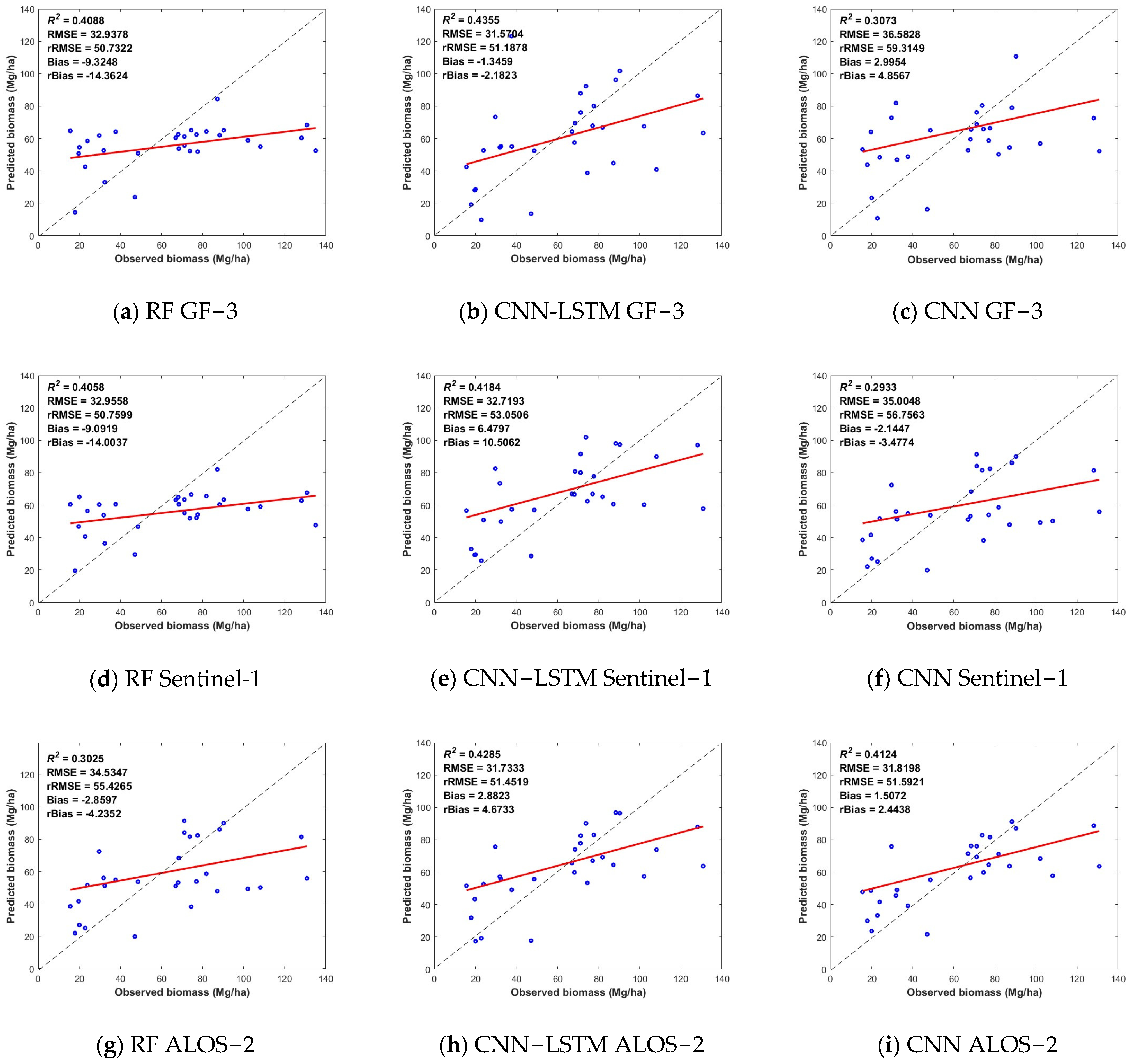
Of the inverse biomass from the three SAR images in Table 11, the biomass estimation from the ALOS-2 image had a higher R2 value and the lowest RMSE; the results from the GF-3 image had the second-best accuracy, and the results from the Sentinel-1 image had the lowest accuracy in all methods. As stated in previous studies, the L-band is more sensitive to forest biomass inversion than the C-band because the wavelength is proportional to the penetration of radar to the forest canopy [37,38]. The short wavelength of the C-band cannot penetrate the dense canopy and basically reacts with the canopy, while the longer wavelength of the L-band can penetrate the vegetation canopy and obtain more vertical information. The better spatial resolutions of the GF-3 and ALOS-2 data may be the other crucial factor that affects the estimate accuracy.
Comparing the different estimation methods, the composite model (CNN-LSTM) performed best, and the CNN model also performed better in inverting the deep learning models. Overall, the two deep learning algorithms examined in the paper had better inversion results compared to the machine learning models. Scatter plots of the prediction results for different methods are shown in Figure 5, in which the RF worked well in this case, probably because RF yields an importance ranking of the factors that provides a better underlying nonparametric model. The composite CNN-LSTM model used the CNN network to obtain deep information about the data and to mine the characteristics of the data, while the LSTM network had a strong memory for obtaining data associations, fully integrating the advantages of both networks in prediction and improving biomass inversion accuracy.
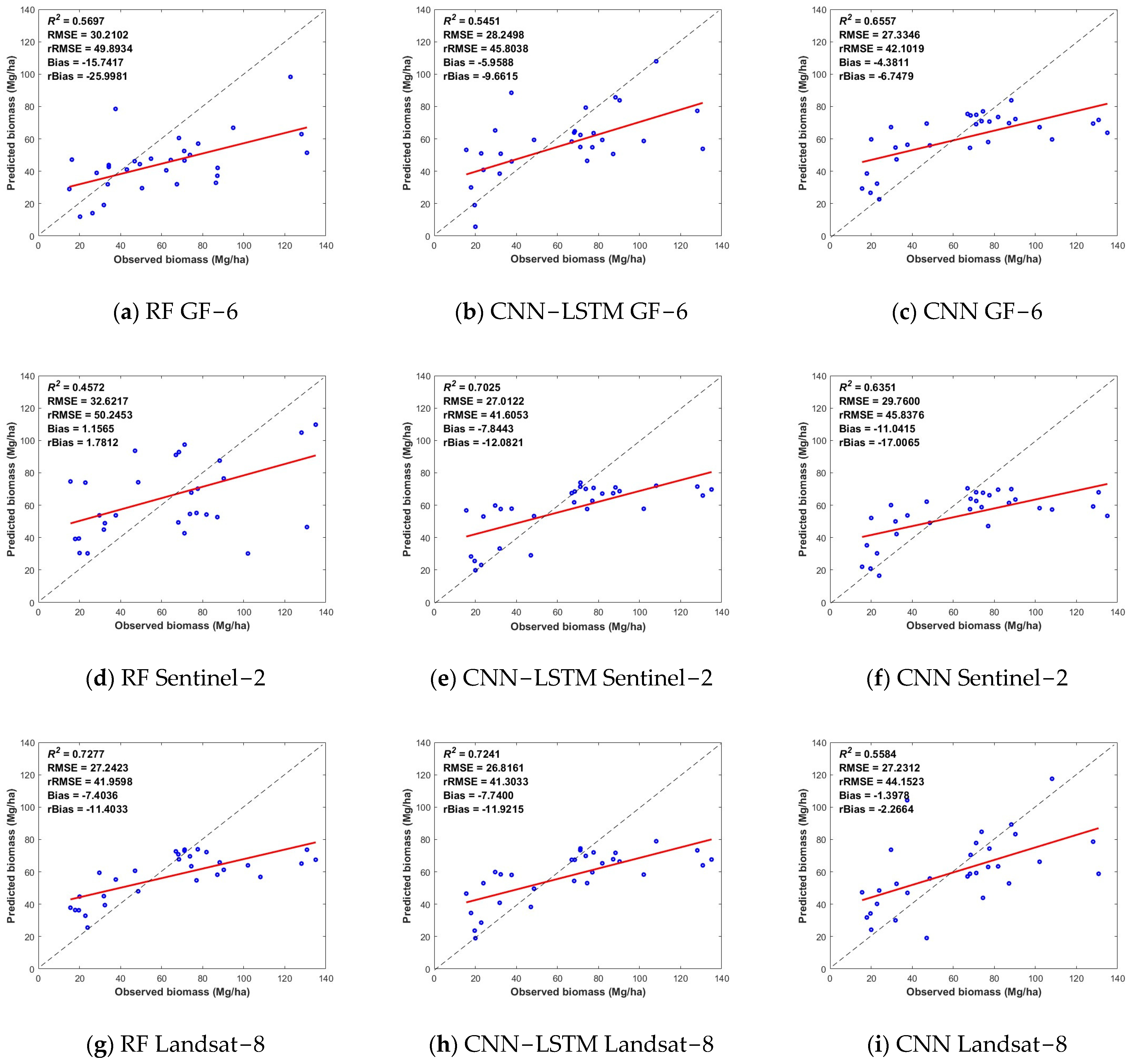
As shown in Figure 6, of the inversion biomass values among the three types of optical images, the biomass estimation results of the Landsat-8 images had relatively high R2 and low RMSE values, with the highest estimation accuracy. The Sentinel-2 images had the second-highest accuracy, and the GF-6 images produced the lowest accuracy estimates.
The results demonstrate the better performance of the composite model (CNN-LSTM), which combines the advantages of both networks, using the unique convolution operation of the CNN network to obtain features from the data and LSTM to obtain the data associations, thus improving the model estimation accuracy. Overall, the two deep learning algorithms had better inversion results compared to the machine learning model.

3.3. Mapping Spatial Distribution of Forest

There is a nonlinear relationship between forest biomass and remote sensing feature variables. Optical instruments can provide finer vegetation spectral spectrums, and SAR sensors are sensitive to structural and electromagnetic information related to slope, shape and surface roughness [39]. By combining optical and radar images, the advantages of each image can be fully explored to achieve data complementarity, thus enhancing the accuracy of the inversion of forest biomass. Considering that data redundancy reduces the accuracy of model inversion, the joint active-passive remote sensing inversion of forest biomass needs to select variables with high correlations with biomass and to fully utilize the individual strong points of different data. To do this, the variables in Table 12 were used.
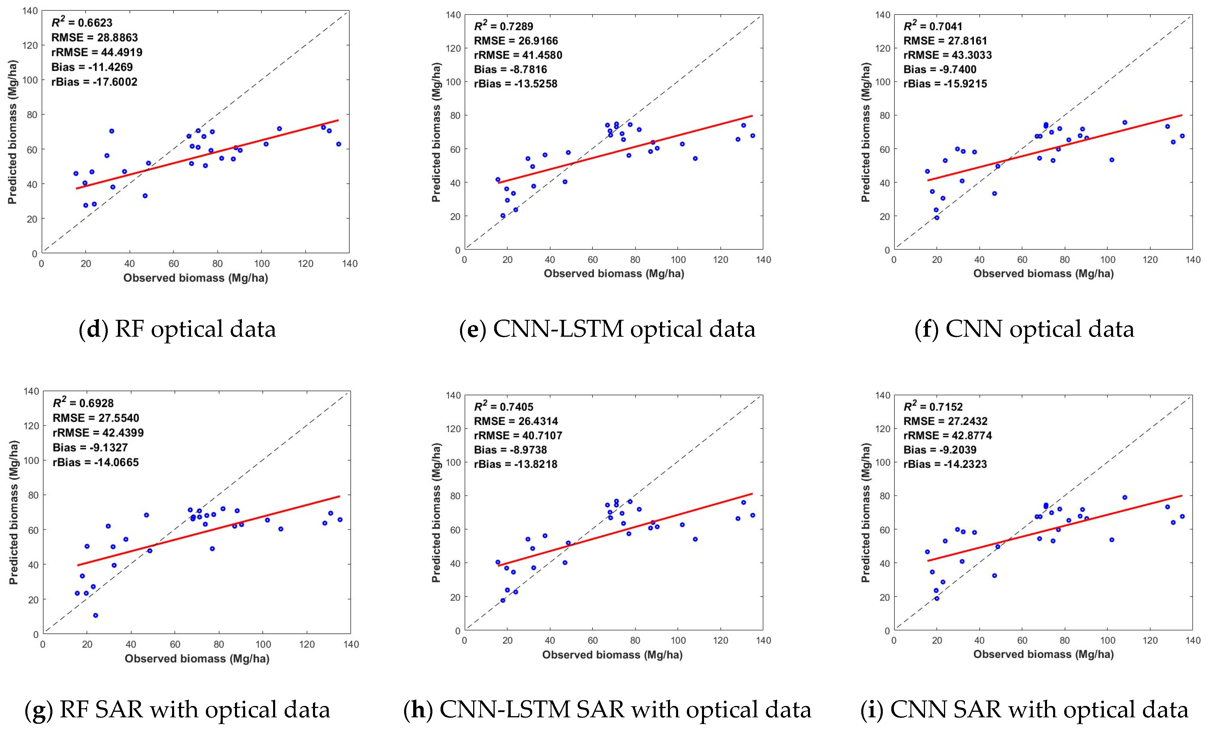
Figure 7 shows the biomass inversion based on different models and data classes. Compared with the single dataset, the combination of SAR and optical images generally significantly improves estimation accuracy and model fit, regardless of the methods used. The R2 of the CNN-LSTM prediction from the multisource data reached 0.7405, and the RMSE reached 26.4314 Mg/ha, indicating the advantage of applying a combined dataset. Second, for the estimation results of the three synergistic optical datasets, the CNN-LSTM model estimated an R2 value of up to 0.7289 and an RMSE of up to 26.9166 Mg/ha. Finally, the inversion results based on SAR datasets and the CNN-LSTM resulted in an R2 of 0.5882 and an RMSE of 30.0384 Mg/ha. The combination of the SAR data did not significantly improve the biomass estimation accuracy, probably because the contrast of SAR features was relatively low [8].
The composite algorithm (CNN-LSTM) had a better accuracy regardless of the combination of multisource data, showing a good-fitting trend to the data. The deep learning estimation results with CNN-LSTM outperformed the RF approach, indicating that combining multisource data with deep learning is feasible for predicting forest biomass.
Considering the best performance of the CNN-LSTM model and multisource datasets, we further developed a biomass estimation model with in situ data. In Figure 8, the spatial distribution of forest biomass was mapped, and the majority of the biomass values in the study area in 2018 ranged from 60 to 90 Mg/ha, with an average value of 64.20 Mg/ha. The low-value areas of biomass were mainly concentrated in the more densely populated eastern and northern regions, while the high-value areas of biomass were mainly located in the sparsely populated remote forest areas and the western regions far from the towns, with a relatively scattered distribution.

4. Discussion

This study explored the potential of multiple remotely sensed images and deep learning algorithms for forest aboveground biomass estimation. In addition to using data from the more popular Sentinel series satellites, Landsat-8, ALOS-2, etc., the experiment also incorporates data from the seldom-used Chinese Gaofen series satellites. The experiment also uses the newly popular advanced CNN-LSTM method. To our surprise, the results from the Gaofen series satellites are very beautiful. This experiment demonstrated the great potential of China’s Gaofen series of satellites to assess the aboveground biomass of forests. In addition, this work achieved good results with a small number of samples by integrating multisource remote sensing data and using the CNN-LSTM method.

4.1. Variable Selection

As involving too many remotely sensed features in modeling can cause information redundancy, correlation analysis between feature variables and forest biomass is needed, and feature variables with strong correlations with biomass are screened. In this paper, the Pearson correlation coefficient method was utilized to perform correlation analysis. Among the feature variables obtained based on C-band GF-3, Sentinel-1 and L-band ALOS-2 data, the dual-polarization decomposition parameters had the highest sensitivity to forest biomass, followed by the texture feature of backscatter and the backscatter coefficient. The backscatter coefficient and texture feature of the L-band ALOS-2 were more sensitive to biomass than those of the C-band due to the penetration capability of L-band wavelengths. Among the features of the optical images, the red-edge band, vegetation index and principal components were strongly correlated with biomass, and the band information and vegetation index were overall more correlated with forest biomass than were the texture features. The main reason for the significant quantitative and correlation advantages over the feature variables of the radar data may be the finer spatial texture information of the high-resolution imagery, while the vegetation red-edge band is very favorable for monitoring plant growth conditions on the ground.

4.2. Comparison of Different Sensors

In Figure 5, the results of the SAR datasets demonstrated that the biomass estimate accuracy of ALOS-2 in the L-band was slightly greater than that of GF-3 and Sentinel-1 in the C-band. This difference was mainly attributed to the penetration and spatial resolution. The L-band can obtain more vertical information due to its capacity to penetrate the crown. The finer spatial resolution, on the other hand, provides more detail and, therefore, has a positive effect. Meanwhile, the aboveground biomass estimation accuracies of Gaofen-3 and Sentinel-1 performed similarly under each model, and even Gaofen-3 slightly outperformed Sentinel-1. However, in Figure 7a–c, it is worth noting that the combination of the three sources of radar data did not significantly improve the accuracy of aboveground biomass estimation. The model with the highest accuracy is the CNN-LSTM model—the R2 was 0.5882, and the RMSE was 30.0384. This result has a large gap with the aboveground biomass estimation results obtained from the combination of the three optical data. This gap may occur because of the lower biomass saturation point of the radar characterization factor.
In Figure 6, comparing the accuracy of aboveground biomass estimation results from optical data, the performance of Gaofen-6 is relatively mediocre. The accuracy of Landsat-8 is the best, with high R2 and low RMSE in both the RF and CNN-LSTM models. In Figure 7d–f, in the CNN-LSTM model, the combination of the three optical data achieves the best among optical data results; the R2 was 0.7289, and the RMSE was 26.9166.
In Figure 7g–i, the accuracy of aboveground biomass estimated by fusing all optical and radar data is basically higher than the accuracy of aboveground biomass obtained from a single data. Among the results, the CNN-LSTM model estimation has the highest accuracy among the 27 results; the R2 was 0.7405, and the RMSE was 26.4314. In addition, among the results of the CNN model, the precision of the results of the fused multisource remote sensing data was higher than the precision of the other data that also used the CNN model. In the RF model, the accuracy of the results of fused multisource remote sensing data was only lower than that of Landsat-8 data. This fully demonstrates the advantage of fused multisource remote sensing data in estimating the accuracy of aboveground biomass. It also demonstrates the potential of China’s Gaofen series of satellites in estimating aboveground biomass.

4.3. Model Comparison

We deployed three methods, i.e., RF, CNN and CNN-LSTM, to estimate forest aboveground biomass. Deep learning methods generally perform better than machine learning methods. Particularly, CNN-LSTM combines the advantages of both the CNN and LSTM algorithms, showing the best ability to fit complex relationships and reduce the misestimation of biomass. In the results of estimating forest aboveground biomass using nine types of data separately, the CNN-LSTM model achieved the best results in eight types of data, and the accuracies were all better than those of the RF model and the CNN model. Therefore, the potential of CNN-LSTM in estimating aboveground biomass is very great and deserves follow-up research.
It should also be noted that the models constructed on the basis of different data and methods generally have the phenomena of high underestimation and low overestimation. As shown in Figure 5, Figure 6 and Figure 7, when the measured forest aboveground biomass is greater than 80 Mg/ha, the aboveground biomass predicted by the model has a large difference from the measured value and is smaller than the measured value, which is a high underestimation. On the contrary, when the measured forest biomass is less than 30 Mg/ha, the aboveground biomass predicted by the model is generally larger than the measured value, which is the low-value overestimation. When the aboveground biomass was measured, it was in the range of 30–80 Mg/ha, and there was less variation in the results of the various model estimates. This may be because in areas with low aboveground biomass, the vegetation cover is lower, and the surface is more exposed. More surface information is included in the information recorded by remote sensing images, which results in a mixing of image pixels and produces a low-value overestimation. In areas with high aboveground biomass, the vegetation cover is higher. When the pixel information is recorded, the remote sensing image tends to be saturated with information, which makes it impossible to estimate excessive aboveground biomass, thus resulting in the phenomenon of underestimation of high values.

5. Conclusions

In this paper, remote sensing modeling estimation of forest aboveground biomass was carried out based on multisource remote sensing data, including mainstream multispectral images (GF-6, Sentinel-2 and Landsat-8) and various SAR data (GF-3, Sentinel-1, ALOS-2 PALSAR-2) in China and abroad. Remote sensing features were extracted, and the Pearson correlation coefficient method was used to select the modeling factors. Forest biomass estimation models were constructed according to various machine learning and deep learning methods, and the estimation accuracies of the different models were compared and evaluated. The results revealed that for the SAR dataset, the biomass estimate accuracy of the L-band ALOS-2 data was higher than that of the GF-3 and Sentinel-1 data in the C-band. Comparing the biomass estimation modeling results of different optical data, the CNN-LSTM model combined the advantages of both the CNN and LSTM algorithms and showed a better ability to fit complicated relationships. Integrating data from different sources to estimate biomass can fully take advantage of these characteristics, complementing the advantages of individual sensors and thus improving the accuracy of the models.

Author Contributions

Conceptualization, X.T. and M.J.; methodology, J.L. and F.Z.; software, H.Z.; validation, X.T.; formal analysis, X.T.; investigation, J.L.; resources, X.T. and M.J.; data curation, X.T.; writing—original draft preparation, X.T.; writing—review and editing, M.J. and J.L. All authors have read and agreed to the published version of the manuscript.

Funding

This research was funded by Provincial and Ministerial Level Key Laboratory Scientific Research Project (grant numbers 2242023K30017); Jiangsu Provincial Key R&D Programme (Social Devel-opment) (grant numbers BE2022820).

Data Availability Statement

Data are contained within the article.

Acknowledgments

The authors thank JAXA for providing the ALOS-2 data and the ESA for providing the Sentinel-1 and -2 images.

Conflicts of Interest

The authors declare no conflicts of interest.

References

  1. Zhang, F.; Tian, X.; Zhang, H.; Jiang, M. Estimation of Aboveground Carbon Density of Forests Using Deep Learning and Multisource Remote Sensing. Remote Sens. 2022, 14, 3022. [Google Scholar] [CrossRef]
  2. Fu, Y. Aboveground biomass estimation and uncertainties assessing on regional scale with an improved model analysis method. Hubei For. Sci. Technol. 2018, 47, 1–4. [Google Scholar]
  3. Zhang, X.; Tian, X.; Chen, E.; He, Q. A review of forest above-ground biomass estimation methods. J. Beijing For. Univ. 2011, 33, 144–150. [Google Scholar] [CrossRef]
  4. Chen, L.; Wang, Y.; Ren, C.; Zhang, B.; Wang, Z. Assessment of multi-wavelength SAR and multispectral instrument data for forest aboveground biomass mapping using random forest kriging. For. Ecol. Manag. 2019, 447, 12–25. [Google Scholar] [CrossRef]
  5. Wu, J.; Fu, G. Modelling aboveground biomass using MODIS FPAR/LAI data in alpine grasslands of the Northern Tibetan Plateau. Remote Sens. Lett. 2018, 9, 150–159. [Google Scholar] [CrossRef]
  6. Li, R.; Liu, J. Application of LandsatETM data to estimate the biomass of wet vegetation in Poyang Lake. J. Geogr. 2001, 56, 531–539. [Google Scholar]
  7. Silva, C.A.; Saatchi, S.; Garcia, M.; Labrière, N.; Klauberg, C.; Ferraz, A.; Meyer, V.; Jeffery, K.J.; Abernethy, K.; White, L.; et al. Comparison of Small- and Large-Footprint Lidar Characterization of Tropical Forest Aboveground Structure and Biomass: A Case Study from Central Gabon. IEEE J. Sel. Top. Appl. Earth Obs. Remote Sens. 2018, 11, 3512–3526. [Google Scholar] [CrossRef]
  8. Ali, I.; Cawkwell, F.; Dwyer, E.; Green, S. Modeling Managed Grassland Biomass Estimation by Using Multitemporal Remote Sensing Data—A Machine Learning Approach. IEEE J. Sel. Top. Appl. Earth Obs. Remote Sens. 2017, 10, 3254–3264. [Google Scholar] [CrossRef]
  9. Shao, Z.; Zhang, L.; Wang, L. Stacked Sparse Autoencoder Modeling Using the Synergy of Airborne LiDAR and Satellite Optical and SAR Data to Map Forest Above-Ground Biomass. IEEE J. Sel. Top. Appl. Earth Obs. Remote Sens. 2017, 10, 5569–5582. [Google Scholar] [CrossRef]
  10. Zheng, D.; Rademacher, J.; Chen, J.; Crow, T.; Bresee, M.; Moine, J.L.; Ryu, S.R. Estimating aboveground biomass using Landsat 7 ETM+ data across a managed landscape in northern Wisconsin, USA. Remote Sens. Environ. 2004, 93, 402–411. [Google Scholar] [CrossRef]
  11. Yue, J.; Yang, G.; Feng, H. Comparative of remote sensing estimation models of winter wheat biomass based on random forest algorithm. Trans. Chin. Soc. Agric. Eng. 2016, 32, 175–182. [Google Scholar]
  12. Zhou, R.; Zhao, T.; Wu, F. Aboveground Biomass Model Based on Landsat-8 Remote Sensing Images. J. Northwest For. Univ. 2022, 37, 186–192. [Google Scholar]
  13. Aguirre-Salado, C.A.; Trevino-Garza, E.J.; Aguirre-Calderon, O.A.; Jimenez-Perez, J.; Gonzalez-Tagle, M.A.; Valdez-Lazalde, J.R.; Sanchez-Diaz, G.; Haapanen, R.; Aguirre-Salado, A.I.; Miranda-Aragon, L. Mapping aboveground biomass by integrating geospatial and forest inventory data through a k-nearest neighbor strategy in North Central Mexico. J. Arid. Land 2014, 6, 80–96. [Google Scholar] [CrossRef]
  14. Hong, Y.; Xu, J.; Wu, C.; Pang, Y.; Zhang, S.; Chen, D.; Yang, B. Combining Multisource Data and Machine Learning Approaches for Multiscale Estimation of Forest Biomass. Forests 2023, 14, 2248. [Google Scholar] [CrossRef]
  15. Singh, C.; Karan, S.L.; Sardar, P.; Samadder, S.R. Remote sensing-based biomass estimation of dry deciduous tropical forest using machine learning and ensemble analysis. J. Environ. Manag. 2022, 308, 114639. [Google Scholar] [CrossRef] [PubMed]
  16. Guerra-Hernández, J.; Narine, L.L.; Pascual, A.; Gonzalez-Ferreiro, E.; Botequim, B.; Malambo, L.; Neuenschwander, A.; Popescu, S.C.; Godinho, S. Aboveground biomass mapping by integrating ICESat-2, SENTINEL-1, SENTINEL-2, ALOS2/ PALSAR2, and topographic information in Mediterranean forests. GIScience Remote Sens. 2022, 59, 1509–1533. [Google Scholar] [CrossRef]
  17. Nandy, S.; Srinet, R.; Padalia, H. Mapping forest height and aboveground biomass by integrating ICESat-2, Sentinel-1 and Sentinel-2 data using random forest algorithm in northwest Himalayan foothills of India. Geophys. Res. Lett. 2021, 48, e2021GL093799. [Google Scholar] [CrossRef]
  18. Shendryk, Y. Fusing GEDI with earth observation data for large area aboveground biomass mapping. Int. J. Appl. Earth Obs. Geoinf. 2022, 115, 103108. [Google Scholar] [CrossRef]
  19. Schreiber, L.V.; Amorim, J.G.A.; Guimaraes, L.; Matos, D.M.; da Costa, C.M.; Parraga, A. Above-ground Biomass Wheat Estimation: Deep Learning with UAV-based RGB Images. Appl. Artif. Intell. 2022, 36, 2055392. [Google Scholar] [CrossRef]
  20. Ghosh, S.M.; Behera, M.D. Aboveground biomass estimates of tropical mangrove forest using Sentinel-1 SAR coherence data—The superiority of deep learning over a semi-empirical model. Comput. Geosci. 2021, 150, 104737. [Google Scholar] [CrossRef]
  21. Narine, L.L.; Popescu, S.C.; Malambo, L. Synergy of ICESat-2 and Landsat for Mapping Forest Aboveground Biomass with Deep Learning. Remote Sens. 2019, 11, 1503. [Google Scholar] [CrossRef]
  22. Tian, L.; Wu, X.; Tao, Y.; Li, M.; Qian, C.; Liao, L.; Fu, W. Review of Remote Sensing-Based Methods for Forest Aboveground Biomass Estimation: Progress, Challenges, and Prospects. Forests 2023, 14, 1086. [Google Scholar] [CrossRef]
  23. Zhu, Y.; Feng, Z.; Lu, J.; Liu, J. Estimation of Forest Biomass in Beijing (China) Using Multisource Remote Sensing and Forest Inventory Data. Forests 2020, 11, 163. [Google Scholar] [CrossRef]
  24. Chrysafis, I.; Mallinis, G.; Siachalou, S.; Patias, P. Assessing the relationships between growing stock volume and Sentinel-2 imagery in a Mediterranean forest ecosystem. Remote Sens. Lett. 2017, 8, 508–517. [Google Scholar] [CrossRef]
  25. Jiang, F.; Sun, H.; Li, C.; Ma, K.; Chen, S.; Long, J.; Ren, L. Retrieving the forest aboveground biomass by combining the red edge bands of Sentinel-2 and GF-6. Acta Ecol. Sin. 2021, 41, 8222–8236. [Google Scholar] [CrossRef]
  26. Laurin, G.V.; Balling, J.; Corona, P.; Mattioli, W.; Papale, D.; Puletti, N.; Rizzo, M.; Truckenbrodt, J.; Urban, M. Above-ground biomass prediction by Sentinel-1 multitemporal data in central Italy with integration of ALOS2 and Sentinel-2 data. J. Appl. Remote Sens. 2018, 12, 016008. [Google Scholar] [CrossRef]
  27. Pan, L.; Sun, Y.; Wang, Y. Estimation of aboveground biomass in a Chinese fir (Cunninghamia lanceolata) forest combining data of Sentinel-1 and Sentinel-2. J. Nanjing For. Univ. (Nat. Sci. Ed.) 2020, 44, 149–156. [Google Scholar]
  28. Shi, J.; Zhang, W.; Zeng, P.; Zhao, L.; Wang, M. Inversion of forest aboveground biomass from combined images of GF-1 and GF-3. J. Beijing For. Univ. 2022, 44, 70–81. [Google Scholar]
  29. Pan, J. A Method for Estimating Above-Ground Forest Biomass by Combining GF-3 PolSAR Data and LANDSAT-8 OLI Data; Northeast Forestry University: Harbin, China, 2020. [Google Scholar]
  30. Breidenbach, J.; Waser, L.T.; Debella-Gilo, M.; Schumacher, J.; Rahlf, J.; Hauglin, M.; Puliti, S.; Astrup, R. National mapping and estimation of forest area by dominant tree species using Sentinel-2 data. Can. J. For. Res. 2020, 51, 365–379. [Google Scholar] [CrossRef]
  31. Ndikumana, E.; Minh, D.H.T.; Nguyen, H.T.D.; Baghdadi, N.; Courault, D.; Hossard, L.; El Moussawi, I. Estimation of Rice Height and Biomass Using Multitemporal SAR Sentinel-1 for Camargue, Southern France. Remote Sens. 2018, 10, 1394. [Google Scholar] [CrossRef]
  32. Jiang, M.; Guarnieri, A.M. Distributed scatterer interferometry with the refinement of spatiotemporal coherence. IEEE Trans. Geosci. Remote Sens. 2020, 58, 3977–3987. [Google Scholar] [CrossRef]
  33. Zhang, X.; Chan, N.W.; Pan, B.; Ge, X.; Yang, H. Mapping flood by the object-based method using backscattering coefficient and interference coherence of Sentinel-1 time series. Sci. Total Environ. 2021, 794, 148388. [Google Scholar] [CrossRef]
  34. Wang, X.; Chen, Y. A CNN-LSTM-based method for predicting the average speed of vehicles on urban roads. J. Qingdao Univ. Technol. 2023, 44, 117–126+140. [Google Scholar]
  35. Sinha, S.; Santra, A.; Sharma, L.; Jeganathan, C.; Nathawat, M.S.; Das, A.K.; Mohan, S. Multi-polarized Radarsat-2 satellite sensor in assessing forest vigor from above ground biomass. J. For. Res. 2018, 29, 1139–1145. [Google Scholar] [CrossRef]
  36. Minh, D.H.T.; Le Toan, T.; Rocca, F.; Tebaldini, S.; Villard, L.; Rejou-Mechain, M.; Phillips, O.L.; Feldpausch, T.R.; Dubois-Fernandez, P.; Scipal, K.; et al. SAR tomography for the retrieval of forest biomass and height: Cross-validation at two tropical forest sites in French Guiana. Remote Sens. Environ. 2016, 175, 138–147. [Google Scholar] [CrossRef]
  37. Kumar, L.; Sinha, P.; Taylor, S.; Alqurashi, A.F. Review of the use of remote sensing for biomass estimation to support renewable energy generation. J. Appl. Remote Sens. 2015, 9, 097696. [Google Scholar] [CrossRef]
  38. Sinha, S.; Jeganathan, C.; Sharma, L.K.; Nathawat, M.S. A review of radar remote sensing for biomass estimation. Int. J. Environ. Sci. Technol. 2015, 12, 1779–1792. [Google Scholar] [CrossRef]
  39. Michelakis, D.; Stuart, N.; Brolly, M.; Woodhouse, I.H.; Lopez, G.; Linares, V. Estimation of Woody Biomass of Pine Savanna Woodlands from ALOS PALSAR Imagery. IEEE J. Sel. Top. Appl. Earth Obs. Remote Sens. 2015, 8, 244–254. [Google Scholar] [CrossRef]
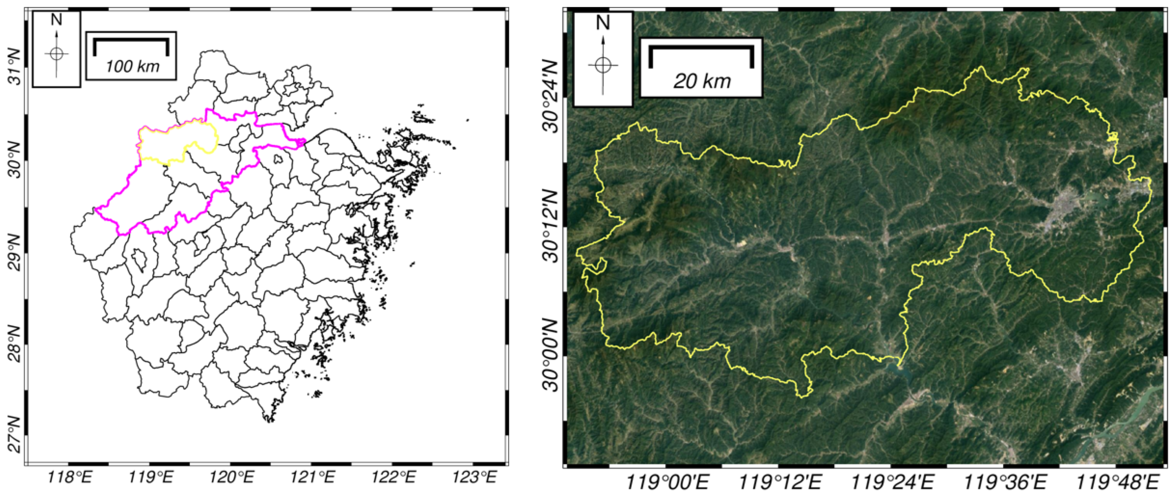
Figure 1. (Left) Location map of the study area in Lin’an district (yellow boundary) of Hangzhou (purple boundary), northwestern Zhejiang Province, China. (Right) Google Maps image of the study area (yellow boundary).
Remotesensing 16 01074 g001
Figure 2. Map of sample plots in the study area.
Remotesensing 16 01074 g002
Figure 3. The flowchart of the research.
Remotesensing 16 01074 g003
Figure 4. Structure of the CNN-LSTM model.
Remotesensing 16 01074 g004
Figure 5. Scatter plot of the biomass prediction results for the RF, CNN-LSTM and CNN algorithms based on radar data. The horizontal coordinates indicate the biomass observations, the vertical coordinates are the predicted values, the dashed black line is the 1:1 straight line, and the red line is the fitted line.
Remotesensing 16 01074 g005
Figure 6. Scatter plot of biomass prediction results from the RF, CNN-LSTM and CNN algorithms based on multispectral data. The horizontal coordinates indicate the observed biomass values, the vertical coordinates are the predicted values, the dashed black line is the 1:1 straight line, and the red line is the fitted line.
Remotesensing 16 01074 g006
Figure 7. Scatter plots of the biomass prediction results of the synergistic inversion of multisource remote sensing data based on the RF, CNN-LSTM and CNN models, where the column indicates the results with the same model but different data source and the row denotes the results from the same dataset but with different models.
Remotesensing 16 01074 g007aRemotesensing 16 01074 g007b
Figure 8. Spatial distribution of the forest aboveground biomass in the study area.
Remotesensing 16 01074 g008
Table 1. Anisotropic growth equations for major tree species in the study area.
Tree SpeciesModel Expressions and Parameters
Fir (Cunninghamia lanceolata (Lamb.) Hook., belonging to the Cupressaceae) W = 0.0492 D 2.660
Horsetail pine (Pinus massoniana Lamb. belonging to the Pinaceae) W = 0.1309 D 2.4367
Hard broad W = 0.0710 ( D 2 H ) 0.9117
Soft broad W = 0.1351 ( D 2 H ) 0.8020
Table 2. Information on the optical data used in the study.
Optical DataData IdentificationCollection TimeProduct LevelSpatial Resolution
GF-6GF6_WFV_E118.4_N29.1_20180905_L1A11198369752018.9.5L1A16 m
Sentinel-2S2B_MSIL1C_20181029T024819_N0206_R132_T50RPU_20181029T0525352018.10.29Level-1Cvisible: 10 m
near-infrared: 20 m shortwave
infrared: 60 m
S2A_MSIL1C_20181110T023921_N0207_R089_T50RQU_20181110T0427432018.11.10Level-1C
Landsat-8LC08_L1TP_120039_20181028_20181115_01_T12018.11.15L1TBands 1–7, 9–11: 30 m
band 8: 15 m
LC08_L1TP_119039_20180911_20180920_01_T12018.9.11L1T
Table 3. SAR data parameters used in the study.
Image TypeAcquisition TimeProduct LevelBandPolarizationSpatial Resolution
GF-317 November 2018L1AC bandHH + HV1 m
Sentinel-11 October 2018
13 October 2018
Level-1C bandVV + VHIW: 5 × 20 m
ALOS-2 PALSAR-225 October 2018
8 November 2018
Level 1.5L bandHH + HVSpotlight: 1–3 m
Stripmap: 3–10 m
ScanSAR: 25–100 m
Table 4. Extraction of waveform information and vegetation indices from multispectral images.
Variable TypeNameDescription
Band InformationGF-6B1, 2, 3, 4, 5, 6
Sentinel-2B2, 3, 4, 5, 6, 7, 8, 8a, 11, 12
Landsat-8B2, 3, 4, 5, 6, 7
Vegetation IndexNDVINDVI = (NIRR)/(NIR + R)
DVIDVI = NIR −R
GNDVGNDV = (NIRG)/(NIR + G)
RVIRVI = NIR/R
Table 5. Extraction of texture feature variables from multispectral images.
NumberTexture Feature NameIntroduction to the Formula
1Mean i j i × m i j
2Variance i j m i j × ( i M e a n ) 2
3Entropy i j m i j lg ( m i j )
4Contrast i j ( i j ) 2 m i j
5Homogeneity i j m i j 1 + ( i j ) 2
6Dissimilarity i j | i j | m i j
7Correlation i j i j m i j μ x μ y σ x σ y
8Second Moment i j ( m i j ) 2
Table 6. Predictors extracted based on SAR data.
Image Data SourceFeature TypeRemote Sensing Predictors
GF-3,
Sentinel-1,
ALOS-2
Backward scattering coefficientGF-3, ALOS-2HH, HV
Sentinel-1VV, VH
Texture featuresMean, Variance, Entropy, Contrast, Homogeneity,
Dissimilarity, Correlation, Second Moment
Polarization decomposition featuresH, A, α
Table 7. Pearson’s correlation coefficients for characteristic variables and biomass for GF-3, Sentinel-1 and ALOS-2 data.
ImageCategoryVariablesPearson’s
Correlation Coefficient
VariablesPearson’s
Correlation Coefficient
GF-3Backward scattering coefficientHH0.069HV0.074
Texture feature factorHH_Mean0.051HV_Mean0.107
HH_Variance0.052HV_Variance0.107
HH_Entropy0.065HV_Entropy0.107
HH_Contrast0.067HV_Contrast0.048
HH_Homogeneity−0.058HV_Homogeneity−0.098
HH_Dissimilarity0.066HV_Dissimilarity0.107
HH_Correlation0.029HV_Correlation−0.064
HH_Second moment−0.032HV_Second moment−0.127
Polarization decomposition parameterH0.271A−0.258
α0.246
Sentinel-1Backscattering coefficientVV−0.002VH0.062
Texture characteristic factorVV_Mean−0.028VH_Mean−0.037
VV_Variance−0.039VH_Variance−0.083
VV_Entropy−0.013VH_Entropy−0.013
VV_Contrast0.32VH_Contrast−0.079
VV_Homogeneity−0.013VH_Homogeneity−0.029
VV_Dissimilarity0.021VH_Dissimilarity−0.006
VV_Correlation−0.077VH_Correlation−0.037
VV_Second moment0.019VH_Second moment−0.017
Polarization decomposition parameterH0.241A−0.238
α0.226
ALOS-2 PALSAR-2Backscattering coefficientHH−0.024HV0.079
Texture factorHH_Mean−0.017HV_Mean0.082
HH_Variance−0.005HV_Variance−0.034
HH_Entropy−0.013HV_Entropy−0.077
HH_Contrast−0.005HV_Contrast0.015
HH_Homogeneity−0.013HV_Homogeneity0.040
HH_Dissimilarity−0.004HV_Dissimilarity−0.007
HH_Correlation−0.045HV_Correlation0.006
HH_Second moment0.031HV_Second moment0.053
Polarization decomposition parameterH0.312A−0.319
α0.235
Table 8. Screening results for biomass predictors based on GF-3, Sentinel-1 and ALOS-2 data.
ImageSelection of Characteristic Variables
GF-3HH_dB, HV_dB, HH_Contrast, H
Sentinel-1VH_dB, VH_Contrast, VH_Variance, A
ALOS-2 PALSAR-2HV_dB, HV_Entropy, HV_Mean, H
Table 9. Pearson’s correlation coefficients for characteristic variables and biomass for GF-6, Sentinel-2 and Landsat-8 data.
ImageCategoryFeature VariablePearson’s Correlation CoefficientFeature VariablePearson’s Correlation Coefficient
GF-6Band informationB10.080B20.036
B30.020B4−0.131
B5−0.118B6−0.092
Vegetation indexNDVI0.091DVI−0.128
GNDV0.01RVI0.206
Texture factorsMean0.084Variance0.141
Entropy−0.048Contrast0.122
Homogeneity0.006Dissimilarity0.041
Correlation0.069Second moment0.083
Principal component analysisPCA10.090PCA20.066
PCA30.343
Sentinel-2Band informationB2−0.291B3−0.332
B4−0.374B5−0.377
B6−0.225B7−0.12
B8−0.157B8a−0.138
B11−0.330B12−0.422
Vegetation indexNDVI0.282DVI0.075
GNDV0.117RVI0.249
Texture factorsMean−0.405Variance−0.111
Entropy−0.216Contrast−0.180
Homogeneity Dissimilarity−0.182
Correlation−0.136Second moment0.155
Principal component analysisPCA1−0.275PCA2−0.368
PCA30.420
Landsat-8Band informationB2−0.273B3−0.402
B4−0.472B5−0.173
B6 B7−0.464
Vegetation indexNDVI0.273DVI−0.028
GNDV0.273RVI0.396
Texture factorsMean−0.348Variance−0.260
Entropy−0.398Contrast−0.211
Homogeneity0.360Dissimilarity−0.324
Correlation0.064Second moment0.374
Principal component analysisPCA1−0.381PCA2−0.371
PCA3−0.406
Table 10. Screening results for biomass predictors based on GF-6, Sentinel-2 and Landsat-8 data.
ImageSelection of Characteristic Variables
GF-6B4, B5, B6, Contrast, Variance, RVI, GNDV, PCA3
Sentinel-2B3, B4, B5, B12, Entropy, Mean, NDVI, PCA3
Landsat-8B3, B4, B7, Second, Entropy, NDVI, RVI, PCA3
Table 11. Results of forest biomass estimation based on GF-3, Sentinel-1 and ALOS-2 data.
Remote Sensing DataEstimation MethodsRMSER2
GF-3RF32.93780.4088
CNN36.58280.3073
CNN-LSTM31.57040.4355
Sentinel-1RF32.95580.4058
CNN35.00480.2933
CNN-LSTM32.71930.4184
ALOS-2RF34.53470.3025
CNN31.81980.4124
CNN-LSTM31.73330.4285
Table 12. Results of the screening of biomass predictors from combined multisource remote sensing data.
ImageSelection of Feature Variables
GF-3HV_dB, HH_Contrast, H
Sentinel-1VH_dB, VH_Variance, A
ALOS-2 PALSAR-2HV_dB, HV_Mean, H
GF-6B5, Variance, RVI, PCA3
Sentinel-2Mean, B12, B5, PCA3
Landsat-8B4, Entropy, RVI, PCA3
Disclaimer/Publisher’s Note: The statements, opinions and data contained in all publications are solely those of the individual author(s) and contributor(s) and not of MDPI and/or the editor(s). MDPI and/or the editor(s) disclaim responsibility for any injury to people or property resulting from any ideas, methods, instructions or products referred to in the content.