Article

Early Detection of Myrtle Rust on Pōhutukawa Using Indices Derived from Hyperspectral and Thermal Imagery

1
Scion, 10 Kyle St, Christchurch 8011, New Zealand
2
Scion, Rotorua 49 Sala Street, Rotorua 3046, New Zealand
3
Environmental Remote Sensing and Geoinformatics, Trier University, 54286 Trier, Germany
*
Author to whom correspondence should be addressed.
Remote Sens. 2024, 16(6), 1050; https://doi.org/10.3390/rs16061050
Submission received: 16 February 2024 / Revised: 9 March 2024 / Accepted: 11 March 2024 / Published: 15 March 2024

Abstract

:
Myrtle rust is a very damaging disease, caused by the fungus Austropuccinia psidii, which has recently arrived in New Zealand and threatens the iconic tree species pōhutukawa (Metrosideros excelsa). Canopy-level hyperspectral and thermal images were taken repeatedly within a controlled environment, from 49 inoculated (MR treatment) and 26 uninoculated (control treatment) pōhutukawa plants. Measurements were taken prior to inoculation and six times post-inoculation over a 14-day period. Using indices extracted from these data, the objectives were to (i) identify the key thermal and narrow-band hyperspectral indices (NBHIs) associated with the pre-visual and early expression of myrtle rust and (ii) develop a classification model to detect the disease. The number of symptomatic plants increased rapidly from three plants at 3 days after inoculation (DAI) to all 49 MR plants at 8 DAI. NBHIs were most effective for pre-visual and early disease detection from 3 to 6 DAI, while thermal indices were more effective for detection of disease following symptom expression from 7 to 14 DAI. Using results compiled from an independent test dataset, model performance using the best thermal indices and NBHIs was excellent from 3 DAI to 6 DAI (F1 score 0.81–0.85; accuracy 73–80%) and outstanding from 7 to 14 DAI (F1 score 0.92–0.93; accuracy 89–91%).

1. Introduction

The extent and impact of invasive fungal pathogens on the world’s forest ecosystems is increasing, in part driven by growing connectivity and human-assisted spread into new areas [1]. Commonly known as myrtle rust, the disease caused by the fungus Austropuc–cinia psidii [2], basionym Puccinia psidii, affects plants in the Myrtaceae family. Native to South and Central America [3,4], invasive strains of the fungus have invaded new areas over the past two decades, having been reported in North America, parts of Asia, Australia, New Caledonia, South Africa and New Zealand [5]. Combined with the pathogen’s wide host range within the Myrtaceae [6,7], the spread of A. psidii has been facilitated by the long-distance dispersal of urediniospores either via wind or anthropogenic movement of spores and infected plant material. This pathogen is a major threat to Myrtaceae in native forest ecosystems as well as myrtle-related industries around the world [8,9,10,11,12].
Due to its impact, and the threat of invasion into new areas by strains currently restricted in range [13], biosecurity restrictions on the movement of Myrtaceae and infected plants are recommended. To minimise the risk of spreading the pathogen, anyone working with or managing Myrtaceae needs to be able to reliably identify infected plants. Field diagnosis of A. psidii requires identification of the host and symptoms. The disease develops on young actively growing tissues while older tissues develop ontogenic resistance to infection [14]. The first visible symptoms appear as distortion, blistering and small purple/red coloured lesions or spots. Eventually, uredinia or telia erupt containing characteristic powdery spores. Identification after visible symptoms have progressed to the stage of uredinia, containing bright yellow spores, is straightforward. However, it is difficult to confirm a diagnosis during the very early stages before uredinia erupt, and not possible during the latent period before symptoms develop. The length of the latent period varies depending on the host and environmental conditions. Under ideal conditions, early symptoms typically occur within 4–7 days and uredinia erupt 5–10 days after infection [14].
The diagnosis of infected Myrtaceae while asymptomatic or with early-stage symptoms is challenging for plant producers. This is particularly the case with large volumes of stock where close visual inspection is unlikely to be practical or cost-effective and may be biased or inaccurate. Diagnosis can be confirmed by examining spores under the microscope or using DNA-based diagnostic assays that can detect the fungus, even in symptomless tissue [15,16,17,18,19]. However, while these methods are easy to apply when sampling is guided by visual detection of symptoms, a random sampling from asymptomatic plants would likely be ineffective and expensive. Hyperspectral and thermal imagery provides a promising method of pre-visual and early disease detection that could be spatially scaled for rapid screening. Physiological responses in plants subject to infection by pathogens often include changes in chlorophyll and other pigments, leaf water content, and key photosynthetic variables such as stomatal conductance, transpiration and photosynthesis that may be detected by shifts in leaf temperature and changes in indices or plant functional traits [20]. Pre-visual or early detection of a range of diseases, in agricultural and forestry crops, have been demonstrated using hyperspectral and thermal imagery at the plant level, often at broad scales [21,22,23,24,25,26].
A recent study [27] found that indices derived from hyperspectral data and thermal imagery were effective under controlled conditions for the pre-visual and early detection of myrtle rust on the model host rose apple (Syzygium jambos (L.) Alston). Excellent pre-visual classification (F1 score range = 0.89–0.94) was achieved from 3 to 1 Days Before Symptoms (DBSs) using narrow-band hyperspectral indices (NBHIs) derived from leaf-level data measured on older resistant leaves using a spectroradiometer. Models using indices derived from thermal imagery could perfectly (F1 score = 1.0) distinguish control plants from myrtle rust-inoculated plants one DBSs were visually detected and through the entire early symptom period. Indices that were most important in models for pre-visual and early detection characterized changes in chlorophyll, water stress and a reduction in leaf temperature, which were associated with measured increases in transpiration. However, the recently developed Lemon Myrtle–Myrtle Rust (LMMR) spectral index [10] for the classification of lemon myrtle (Backhousia citriodora F. Muell. 1859) leaves with advanced disease symptoms was not a significant predictor of pre-visual or early symptoms on rose apple. These findings reinforce the need to test the utility of hyperspectral and thermal indices for the detection of myrtle rust on a range of Myrtaceae and at different stages of disease development. Further research should use canopy-level, rather than leaf-level, hyperspectral data, as this matches the scale of imagery acquisitions when these models are applied for detection purposes within a nursery.
Pōhutukawa (Metrosideros excelsa Sol. ex Gaertn.) is an endemic tree growing up to 25 m, predominantly found in coastal vegetation in northern Aotearoa New Zealand [28]. Of great historical and cultural significance to Māori [29,30], pōhutukawa is also revered as the ‘New Zealand Christmas Tree’ due to the proliferation of red flowers produced in December-January [28]. Planted outside of its natural range in urban areas, pōhutukawa is a native myrtle commonly stocked and propagated in nurseries throughout New Zealand [31]. Having undergone a significant decline following human settlement, the remaining natural pōhutukawa stands are threatened by invasive species and land use change [28]. The most recent threat to pōhutukawa is the pandemic strain of A. psidii, first detected on the New Zealand mainland in 2017, on pōhutukawa at a nursery in the North Island, that has since spread rapidly through its predicted climatic range [32,33,34]. In New Zealand, the current recorded host range for A. psidii (including native, exotic and hybrid taxa) comprises 36 Myrtaceae [35], of which pōhutukawa is one of the most frequently reported hosts [33].
This study examines the accuracy of indices derived from thermal and visible near-infrared (VNIR) hyperspectral imagery to detect myrtle rust on pōhutukawa plants, growing in a controlled environment. The objectives of this research were to (i) identify the key thermal and narrow-band hyperspectral indices (NBHIs) associated with pre-visual and early expression of myrtle rust on pōhutukawa and (ii) develop a classification model to detect the disease.

2. Materials and Methods

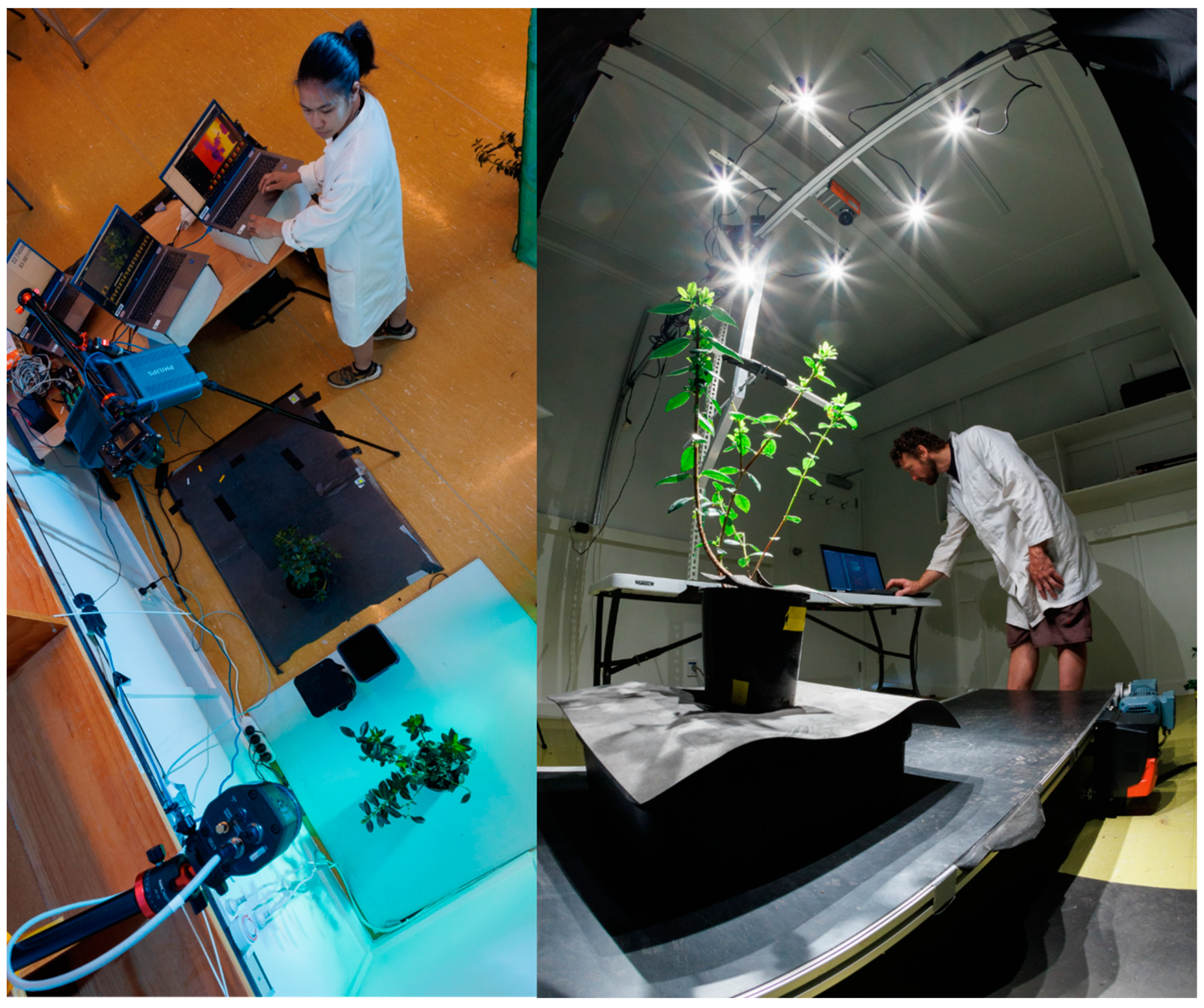
2.1. Experimental Setup

The experiment was undertaken within a dark room in which environmental conditions were regulated from late November to mid December 2023 at Scion (Rotorua, New Zealand). A total of 80 healthy pōhutukawa, that did not show any visual signs of infection, were selected for the experiment. These plants, which were sourced from a Rotorua nursery, were grown in 2.5 litre pots and averaged 35 cm in height at the initiation of the experiment. The plants were well watered by hand over the course of the experiment.
The plants were randomly allocated to a control and a myrtle rust (MR) treatment group on the 29th November. These two groups were separated into different plastic enclosures that had misting capability. Over the measurement period, the following conditions were maintained within each enclosure: 16 h photoperiod under 30 W LED 3000 K grow lights, 22 °C temperature, and relative humidity of 70–80%. The plants remained under the enclosures for most of the time and were only briefly removed for measurements. Within the room, the environmental conditions were similar to those of the enclosure and relatively constant, with an average air temperature of 22 °C and relative humidity of 61%.
During the measurement period, four of the control plants developed minor symptoms and were immediately removed from the enclosure. One of the plants allocated to the MR treatment developed symptoms of another disease and was also removed from the enclosure. Following these removals there were a total of 75 plants used for analyses, of which 26 plants were allocated to the control and 49 plants were allocated to the MR treatment. No further MR symptoms were observed on remaining control plants for 7 days after measurements ended, so they were considered disease-free.
Following the method described in [27] the plants in the MR treatment were inoculated on the 4th December 2023. Inoculum used in the experiment was mass-produced on rose apple and harvested using a portable vacuum pump (Mini Cyclone Spore Collector, Tallgrass Solutions, Manhattan, KS, USA) into 00 gelatin capsules and stored for 24 h at low humidity over silica beads. Prior to inoculation, urediniospores were suspended in a solution comprising 0.05% Tween 20 in sterile distilled water, achieving a concentration of 1 × 10⁵ spores/mL, as quantified using a haemocytometer. The inoculum was uniformly dispersed across the surfaces of young leaves and stems utilizing a gravity-fed airbrush connected to a compressor, operating at a pressure of 2 bar. Subsequent to inoculation, plants were relocated to the enclosures, where they were kept in darkness at a temperature of 18 °C and a relative humidity exceeding 90% for a duration of 24 h to foster optimal infection conditions. Control plants received a mock inoculation employing a sterile 0.05% Tween 20 solution, with all environmental conditions mirrored to eliminate any potential physiological discrepancies attributable to environmental alterations between treatment groups. Following this process, conditions in the enclosures for plants in both the control and MR treatment were returned to a 16 h photoperiod, 22 °C and a relative humidity of 70–80% for the remaining duration of the experiment.
Pre-inoculation measurements were taken from both treatments on the 29th November. Following inoculation, daily measurements were taken from 3–8 days after inoculation (DAI), with a final measurement made 14 DAI on the 18th December. Of the 49 MR plants used within the analyses, the number of symptomatic plants increased rapidly from 3 plants (at 3 DAI) to 12 (4 DAI), 47 (5 DAI), 48 (6 DAI), and 48 (7 DAI), with all 49 plants showing symptoms by 8 DAI.

2.2. Visual Assessment of Symptoms

Following the method described in [27], we recorded the presence or absence of signs and symptoms for each new leaf and stem, that was distinguishable from mature growth in colour and texture. These symptoms included slight bumps or blistering on the leaf surface, red/purple spots, yellow discolouration, and developing pustules yet to break through the epidermis or fully emerged pustules with spores erupted on the surface.

2.3. Thermal Measurements

Canopy-level thermal data were captured using an infrared thermal camera (FLIR A700SC, Teledyne FLIR LLC, Wilsonville, OR, USA). This instrument is characterized by a spectral sensitivity spanning 7.5 µm to 14 µm and can detect thermal gradients as subtle as 30 mK. The imaging resolution of the camera is 640 by 480 pixels. The thermal camera was mounted on a 2 m high tripod, directly above the plant, with a nadir orientation. FLIR Research Studio (Version 3.2.0) was used to control the camera (Figure 1).
Imagery was acquired in a 32-bit TIFF format. To enhance the precision of each data capture, air temperature, relative humidity, emissivity, and target distance were input into the Research Studio software, version 3.2.0. The target distance was set as 2 m and following [26], the emissivity was set to 0.98. The ambient air temperature and relative humidity for the surrounding environment was determined using an HMP155A probe (Vaisala, Vantaa, Finland) connected to a CR1000 datalogger (Campbell Scientific, Logan, UT, USA) that took continuous measurements of these variables at a 1 min interval.
Two calibration targets were positioned either side of the plant within the thermal camera field of view (Figure 1, shown immediately to the left of the bottom right plant). One of these targets consisted of a container with damp soil while black cotton cloth was stretched across the top of the other container. During the capture, the temperatures of these calibration targets were measured using the thermal camera and a handheld IR thermometer. Linear regression was used to develop a relationship between the temperature recorded by the camera (x-variable) and thermometer (y-variable) using data pooled by capture day. This regression was used during post-processing to calibrate the measurements of canopy temperature made by the camera.
The canopy of each individual plant was delineated using object-based image segmentation algorithms incorporated within the Fiji module of ImageJ software, version 1.53t [36]. For every image captured, the average temperature across the segmented crown area was determined. These canopy temperatures were then used as the independent variable (x variable) in the previously described calibration equation to predict the calibrated canopy temperature, denoted as Tc. These Tc values were then paired with the ambient air temperature, Ta, that was concurrently recorded with each measurement and used to determine, for each tree, the normalised canopy temperature, as TcTa.

2.4. Hyperspectral Measurements

2.4.1. Data Acquisition

Plant-level hyperspectral data were acquired on all measurement dates under artificial lighting across the visible near-infrared (VNIR) range using a FX10 hyperspectral camera (Specim, Spectral Imaging Ltd., Oulu, Finland). This push-broom camera captures 448 bands across the 400–1000 nm range with a full width half maximum of 5.5 nm and spectral sampling interval of 2.7 nm. The FX10 has a high signal-to-noise ratio of 600:1 and the spectral sampling includes 1024 pixels captured within a 38° field of view.
Images were recorded in nadir view and the camera was mounted 2 m above the ground on a cross beam (Figure 1). A conveyor belt was used to move the plants through the field of view. The speed of the conveyor belt was adjusted to fit the frame rate of the camera, which in turn was dependent on the exposure time. During the measurements, the conveyor belt speed and frame rate were kept constant and the exposure time was adjusted to avoid over or undersaturation. A diffuse white reference standard (Spectralon, North Hutton, NH, USA) was placed so that it was visible in every frame, allowing calibration of the imagery as a function of the changing illumination conditions.
The conveyor was located inside the dark room and six ASD illuminator reflectance lamps (Malvern Panalytical technologies, Worcestershire, UK) mounted on the frame were used to light the scene (Figure 1). Each of these lamps is a quartz–tungsten–halogen light source with an integrated reflector and in combination they provided stable illumination across the 350–2500 nm range.

2.4.2. Processing of Data and Extraction of Narrowband Hyperspectral Indices

All pre-processing of the hyperspectral data was carried out using Matlab (The MathWorks, Inc., Natick, MA, USA) following the methods described in [37]. The white reference bar was placed close to the edge of the field of view in the hyperspectral images. The brightest pixels in each image line belonged to the white reference bar. These were used to convert digital numbers to reflectance factors by dividing all values by the mean of the five brightest pixels and multiplying the result by the white reference reflectance. Due to wavelength shifts across the field of view, the reflectance signal was distorted. An additional hyperspectral image of a white reference plate filling the complete field of view using the same geometric set-up was recorded. Dividing this image by its own values at the same column numbers where the white reference bar had been detected in the original image resulted in a correction spectrum that could be used to remove the distortions from the reflectance signals [37].
In the corrected reflectance images, pixels containing vegetation were identified using two simple rules: Pixels with NDVI ≥ 0.4 and reflectance at 780 nm ≥ 0.1 were selected as vegetation pixels. The resulting masks were checked visually and coincided well with the plant material. The mean spectrum for all vegetation pixels was extracted and used for further analyses. Following this masking, the plant level spectra were interpolated to a 1 nm resolution from 397–1004 nm. Narrow-band hyperspectral indices (NBHIs) that have been linked to the xanthophyll pigment, red/green/blue bands, plant disease, water content, curvature index and plant structure were derived from the VNIR spectral region for use in analyses. Equations and references for these 81 NBHIs are given in Table A1.

2.5. Physiological Measurements

Physiological measurements were taken prior to inoculation on the 28th November and from symptom-free leaves, after inoculation on the 13th December at 9 DAI. A subset of the total plants was measured on both dates over the course of one day, with pre-inoculation and post-inoculation measurements comprising, respectively, 22 and 26 Control plants and 28 and 31 MR plants. Photosynthetic parameters, including net photosynthetic rate (A), stomatal conductance (gs), and transpiration rate (E), were quantified using the GFS-3000 gas exchange analyser (M-Series, Heinz Walz GmbH, Effeltrich, Germany) following a pre-illumination period of 120 s, under an ambient carbon dioxide concentration of 400 ppm. The GFS-3000 gas exchange analyser was connected to an Imaging-PAM chlorophyll fluorometer (Heinz Walz GmbH, Effeltrich, Germany) and was equipped with a supplementary CO2 cartridge to ensure stable CO2 levels during the measurements.

2.6. Data Analysis

2.6.1. Treatment Differences in Measured Variables

All analyses described in this section were undertaken using R version 4.2.3. [38]. Reflectance was plotted against wavelength, by treatment, for all captures, and a t-test was used to identify the wavelengths with significant treatment differences for each capture. Differences between treatments for all 83 hyperspectral and thermal indices were examined using a t-test for all post-inoculation captures and p values for all these tests were documented. Boxplots showing treatment variation against DAI for the variables that most frequently differed between treatments, or were most important in the classification model (see Section 2.6.2), were constructed. A t-test was used to determine if there were significant treatment differences for each of the physiological variables during both measurement dates.

2.6.2. Classification Model

Random forests was used to classify the two treatments (Control, MR plants) from the measured thermal and hyperspectral indices using scikit learn, version 0.23.2. [39] which was implemented in python. Random Forests is an ensemble learning method that creates a collection of decision trees during training. Each tree in the forest is built from a sample drawn with replacement (bootstrap sample) from the training set, and split decisions are made at each node based on a random subset of the features. This approach enhances diversity among the trees, which reduces overfitting and improves generalisation to unseen data. The final classification decision is made based on the majority voting principle, where the class label predicted by the majority of the trees is chosen as the final output, thereby enhancing the accuracy and robustness of the model.
Separate random forests models were created using data for each of the seven post-inoculation measurement dates, with features comprising either (i) the two thermal indices, (ii) the 81 NBHIs or (iii) the thermal indices and NBHIs. Thus, there were 21 classification models created that included the factorial combination of the seven measurement dates and three sets of predictor variables.
Prior to model fitting, recursive feature elimination (RFE) was used with the random forest algorithm to subset the predictors to the most important variables for each of the 14 models that included either NBHIs or thermal indices/NBHIs. The RFE undertook a stratified cross validation and was constrained so that no more than 10 features, that had correlations of <0.9, were selected to avoid redundancy and overfitting in the final models. Both thermal indices were included in the seven thermal models as there was little collinearity between these variables for all DAI (R2 ≤ 0.06). The final variables included in the models are shown in Table 1. The number of variables for models with NBHIs and NBHIs/thermal indices, ranged from, respectively, 4–8 (mean = 6) and 1–8 (mean = 5).
Following feature selection for each model, a stratified split (with respect to treatment) was used to divide observations into a training dataset comprising 80% of the observations (60 data points) with the remaining 20% (15 observations) retained as a test dataset. The random forest model was fitted to the training dataset using a stratified cross validation with predictions from this fitted model made on the independent test dataset. This process was repeated 49 times using a different train/test split during each iteration, and performance statistics were averaged over predictions on all 50 test datasets. This approach removed any potential bias that may have resulted from an unbalanced choice of test dataset using a single train/test split providing a more rigorous evaluation of true model performance.
Three hyperparameter grids were evaluated for model fitting that varied in complexity, with the simplest using default parameters and the most complex optimising model performance across a range in five parameters (number of estimators, max depth, max features, min samples split, min samples leaf). Decisions around which of these three hyperparameter grids to use for each of the 21 models were based on mean model performance extracted from the 50 iterations on the test dataset to ensure generality. For almost all of the 21 models the default hyperparameter grid resulted in the best model performance.
Using the mean predictions made on all 50 independent test datasets, a confusion matrix was constructed for each model. As is common practice in experiments where disease is predicted [40], the MR plants were designated positive and values in the confusion matrix quantified the percentage of true positives (TPs), true negatives (TNs), false positives (FPs) and false negatives (FNs).
As the dataset was unbalanced, model performance was predominantly assessed using precision, recall and the F1 score (for equations see [27]). Precision quantifies the fraction of correct positive predictions whereas recall identifies the fraction of true positives that were accurately detected. High values of precision mean there are few false positives while high values of recall indicate low numbers of false negatives. The F1 score represents the harmonic mean of precision and recall, serving as a balanced measure of the model discriminatory power. F1 scores span a continuum from 0 to 1, with categorizations from 0.5 to 0.7, 0.7 to 0.8, 0.8 to 0.9, and >0.9 signifying poor, acceptable, excellent, and outstanding levels of discrimination, respectively.
Accuracy is defined as the ratio of correctly predicted observations to the total observations examined. While accuracy is not as useful as the F1 score for evaluating model performance using unbalanced datasets, this metric was incorporated into the analysis to provide a comprehensive assessment.

2.6.3. Relationships between Physiological Variables and Indices

Using the post-inoculation data, linear models were constructed between the three physiological variables (gs, E and A) and the 83 hyperspectral and thermal indices listed in Table A1 (i.e., 249 models comprising 3 dependent variables × 83 predictor variables). Model strength was assessed for all relationships that were significant using the coefficient of determination (R2).

2.7. Software Used

The software that was used within the analyses is shown in Table 2.

3. Results

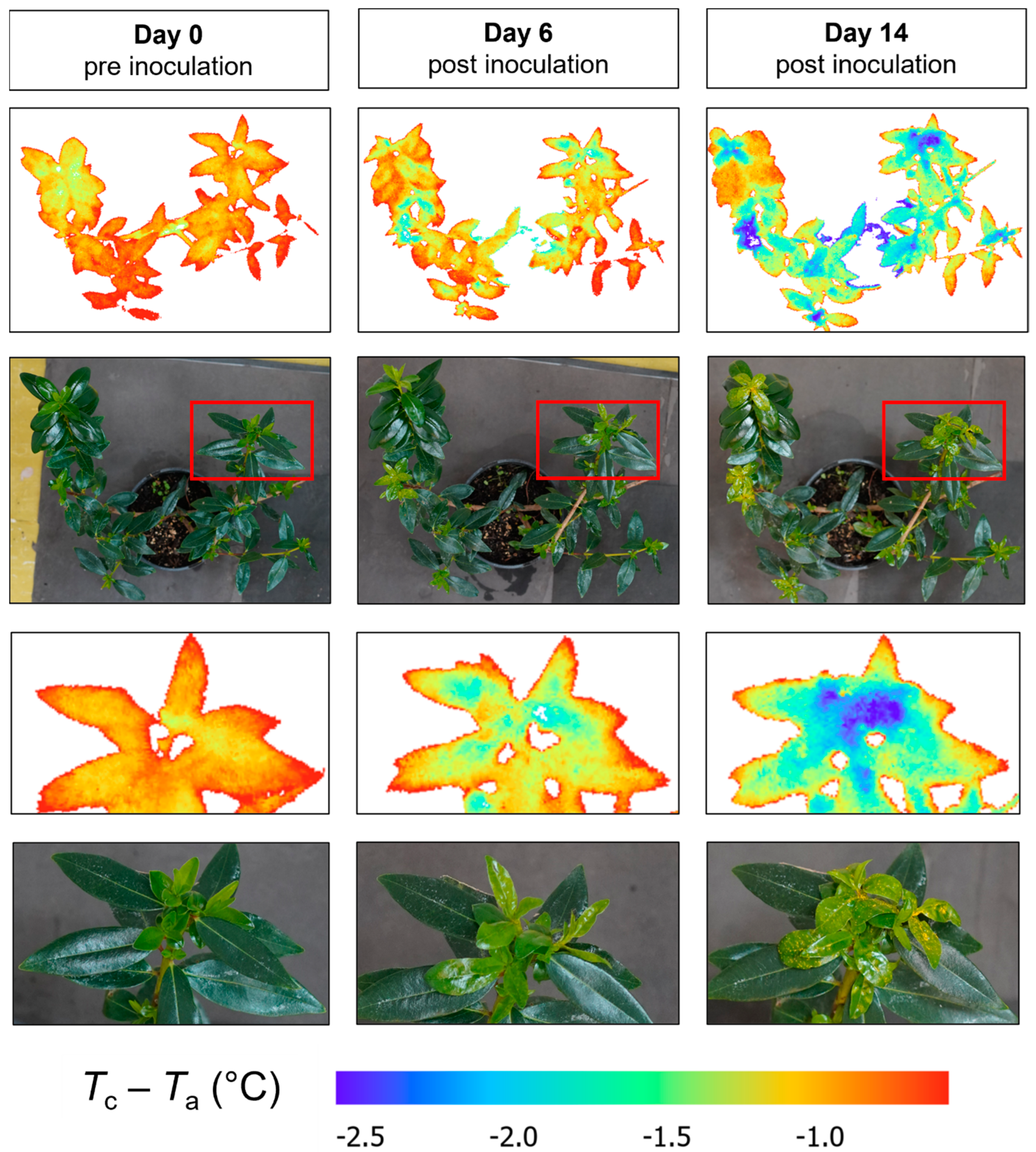
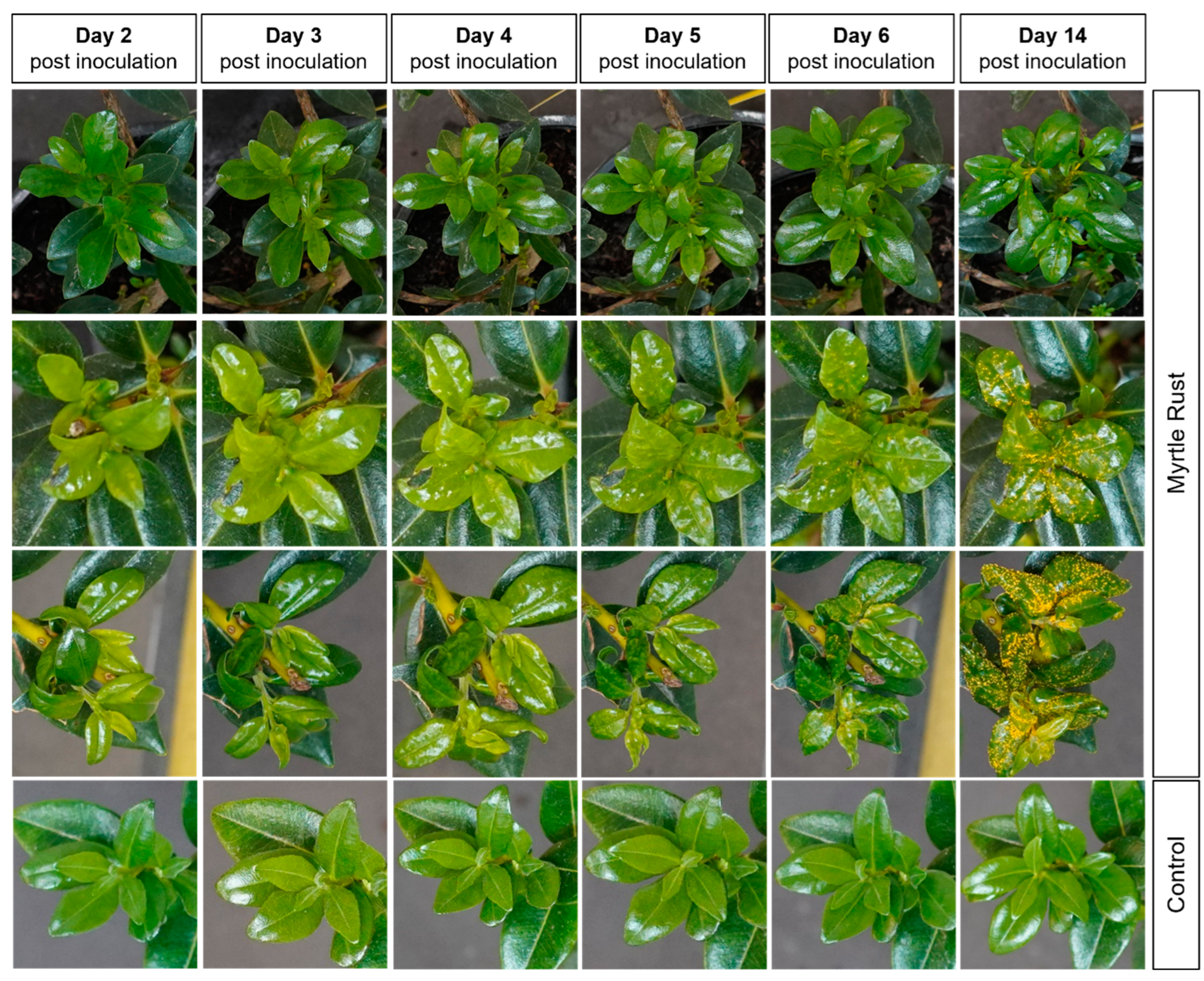
3.1. Disease Symptoms

The first symptoms occurred 3 DAI and by 8 DAI all plants were symptomatic. Between 3 and 5 DAI only bumps were observed. These bumps typically became pronounced and sometimes developed yellow chlorotic colouration between 4 and 5 DAI. There were no red spots or lesions observed at any stage during the experiment. Pustules were developing between 4 and 5 DAI and open from 6 DAI onwards. The extent and severity of symptoms varied widely between plants, and the proportion of new leaves on each plant with symptoms typically increased over time, as did the area with symptoms on leaves and stems (Figure 2).

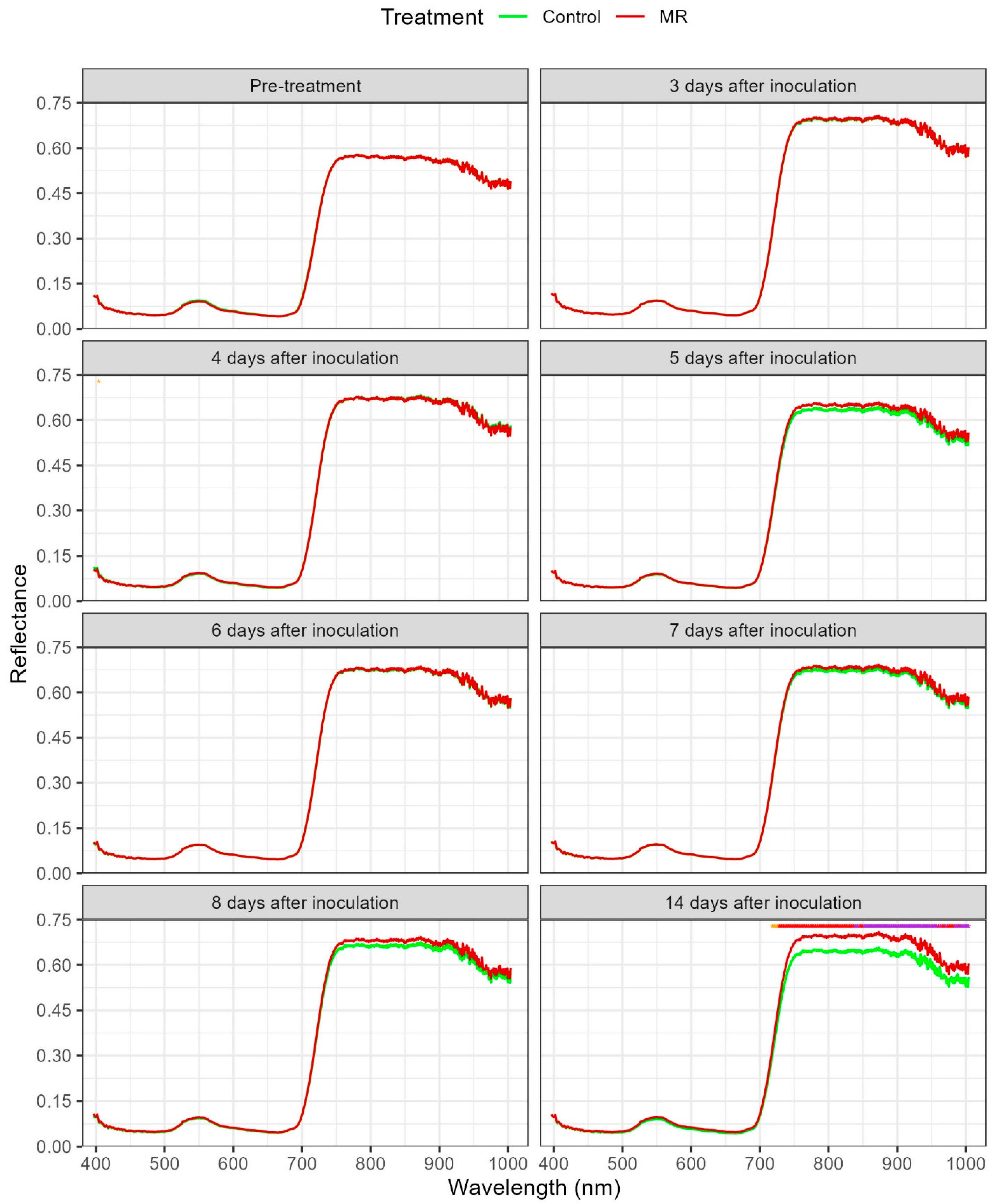
3.2. Hyperspectral Spectra

Very little treatment variation was noted in plant level reflectance across the wavelength range for pre-treatment or post-treatment measurements at 3 and 4 DAI. For measurements taken at 5, 7 and 8 DAI, there was slight treatment divergence in reflectance above the upper end of the red edge at ca. 740 nm with values in the MR treatment exceeding those in the control (Figure 3). These differences in mean reflectance diverged markedly over this spectral range at 14 DAI with values for plants in the MR treatment exceeding those of control plants most markedly at 912 nm. Apart from significant treatment differences at 4 DAI that occurred at 404 nm, significant differences between the treatments were not noted until 14 DAI (Figure 3). At 14 DAI, highly significant differences were noted and this significance generally increased with wavelength, reaching p = 0.05 by 718 nm and p = 0.001 by 839 nm (Figure 3).

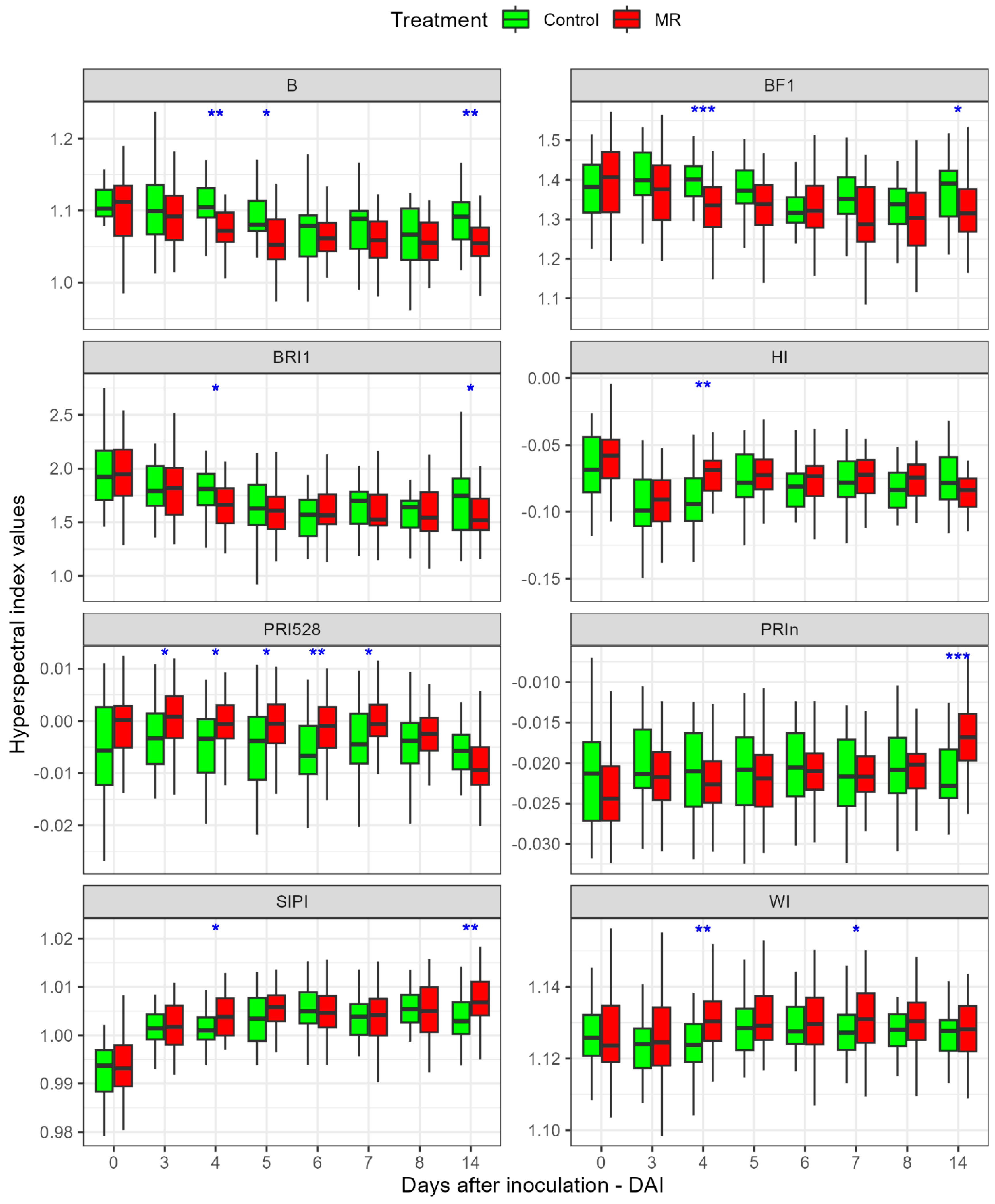
3.3. Variation in Indices between Treatments

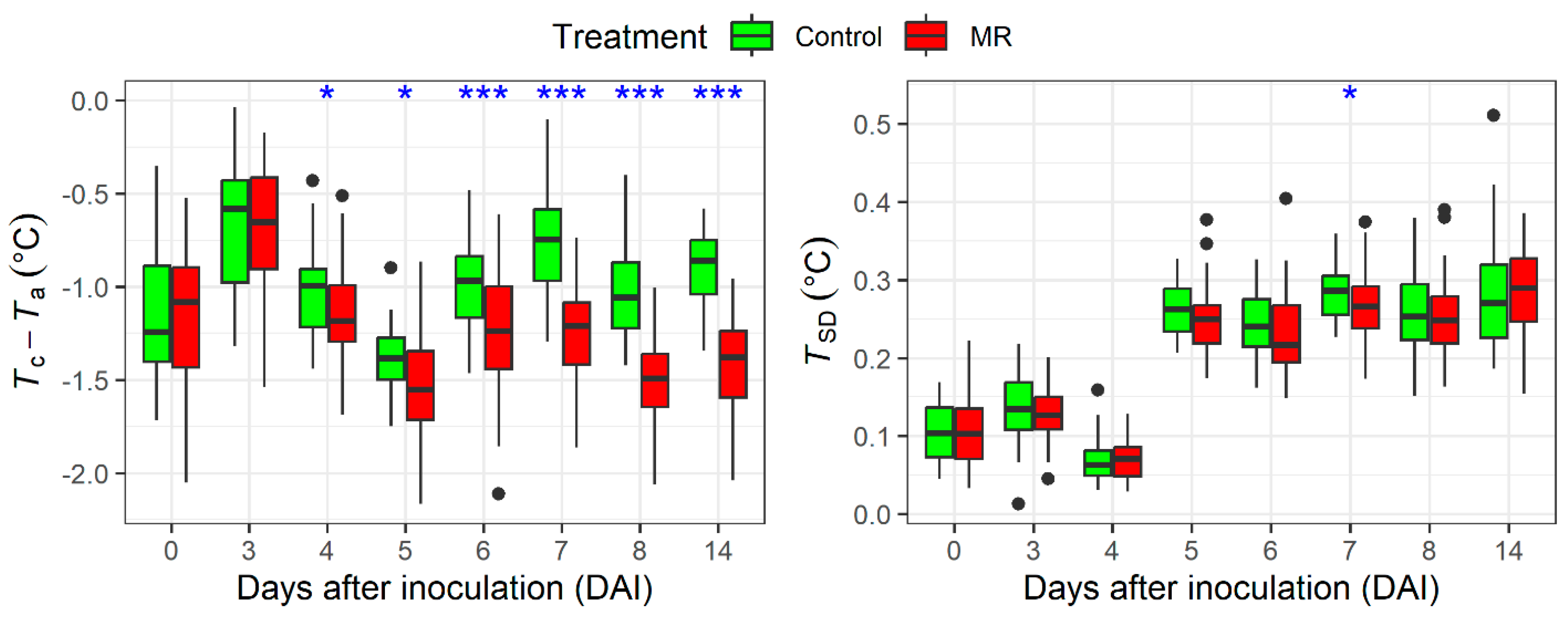
3.3.1. Thermal Indices

There were no significant differences between the two thermal indices during the pre-treatment measurements or those taken at 3 DAI (Figure 4). However, by 4 DAI values of TcTa for plants in the MR treatment were significantly lower than those of the control by 0.16 °C (−1.17 vs. −1.01 °C). This divergence in TcTa increased over the remaining measurements with differences becoming highly significant by 6 DAI (Figure 4). Treatment differences in TcTa were highly significant from 7–14 DAI (p range of 1.5 × 10⁻¹⁰–4.9 × 10⁻¹²), during which time they exceeded 0.49 °C and over this period these treatment differences were most significant among all 83 examined indices (Table A2). Visual changes in TcTa over the course of the experiment (Figure A1) for an example MR plant, show the appearance of cooler regions by 6 DAI, which extended markedly and became far cooler by 14 DAI. These reductions in TcTa were most pronounced for new foliage that is symptomatic (Figure A1) but smaller reductions in TcTa also occurred for older foliage that did not develop symptoms (Figure A1).
In contrast, little systematic variation was noted between treatments for TSD across the measurement range. Values of TSD in the control did exceed those in the MR treatment between 5 and 8 DAI, with these differences becoming significant on 7 DAI. However, by 14 DAI, values of TSD in the MR treatment were higher than those of the control, but this difference was not significant (Figure 4).

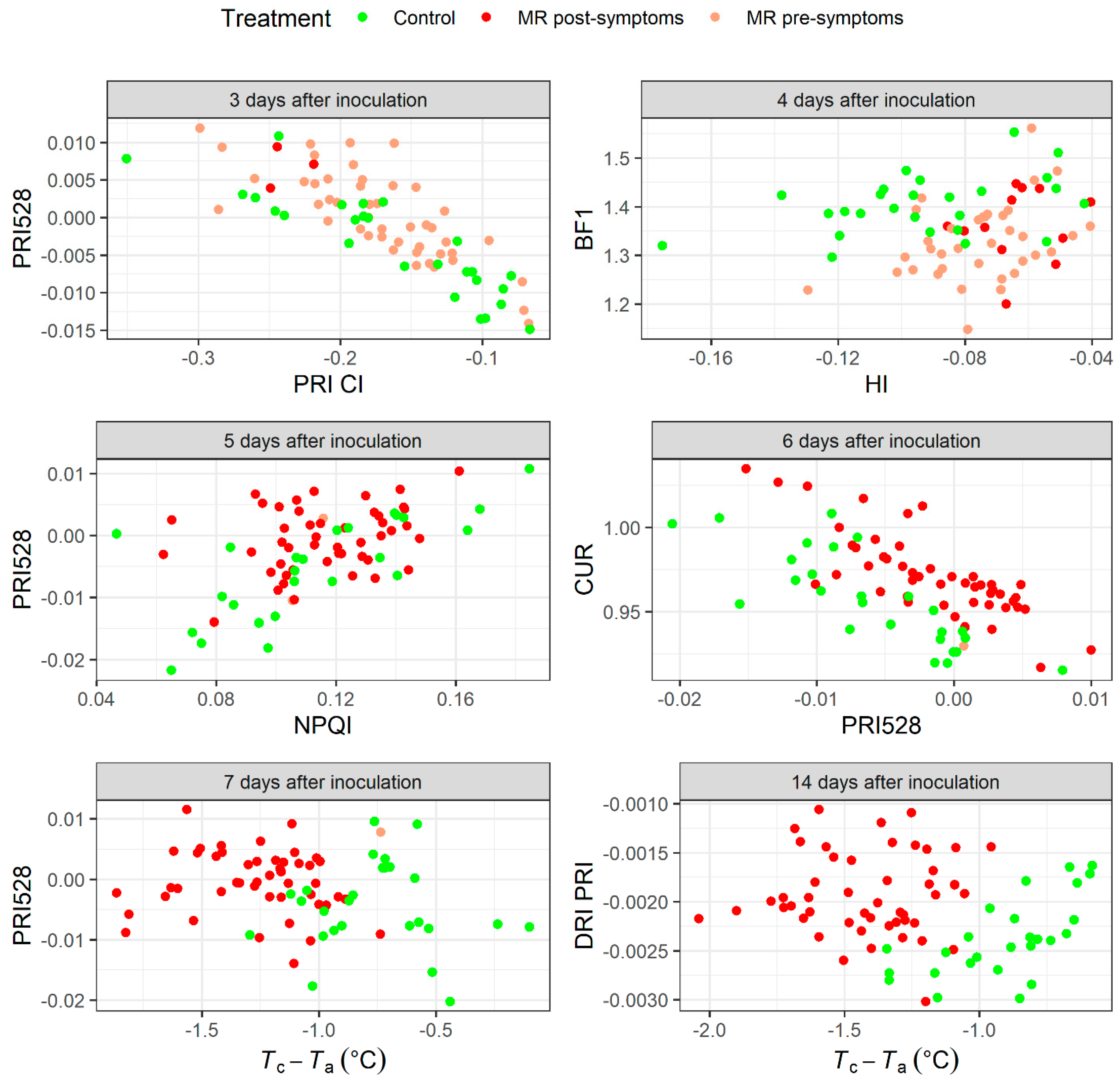
3.3.2. Hyperspectral Indices

Although there was wide variation within each grouping, the xanthophyll indices were generally most sensitive to infection by the pathogen (Table A2). Of all the hyperspectral indices, PRI528 significantly differed the most frequently between treatments. Values of PRI528 were significantly higher within the MR treatment than the control during five measurements dates from 3 to 7 DAI, but converged after this time, with values in the control exceeding those in the MR treatment, but not significantly so, by 14 DAI (Figure 5). Although the other xanthophyll indices did not significantly differ from 3 to 8 DAI, many of these indices exhibited highly significant treatment differences at 14 DAI (Table A2). Among these, treatment differences for DRI PRI and PRIn were most significant (p ≤ 4.2 × 10⁻⁵) among all hyperspectral indices, with values of PRIn in the MR treatment exceeding values in the control at this time (Figure 5).
Most of the indices in other hyperspectral categories were relatively insensitive to treatment from 3 to 8 DAI. However, there were quite a few indices, split across a number of categories, that exhibited highly significant differences between treatments at 4 DAI (Table A2). Among these, the indices that differed most significantly included all three water indices (fWBI, WBI, WI), healthy index (HI), and indices that included reflectance in the blue band (B, BGI, BRI, BF indices and to a lesser extent SRPI, NPCI, SIPI). For a selection of these key indices values in the MR treatment were elevated above control values for SIPI, WI, HI, but reduced below control values for the blue indices, B, BF1 and BRI1 (Figure 5). By 14 DAI, many hyperspectral indices in these categories significantly differed between treatments. Although there were no significant treatment differences for any of the structural indices before this time (Table A2), there were significant differences between treatments for over half (8/15) of these indices at 14 DAI, with the most significant differences occurring for RDVI, TVI, MTVI1, MCARI1 and EVI (p < 0.01). Within other categories, the most significant treatment differences were noted for B, BRI2, CLS and SIPI (p < 0.01), but as previously mentioned, none of these differences were as strong as those noted for xanthophyll indices at 14 DAI.

3.4. Model Predictions

3.4.1. Models Using Thermal Indices

The developed models had low to moderate performance for data obtained during 3 and 4 DAI, with accuracy < 62% and an F1 score of 0.75 over these two measurement dates (Table 3). However, by 5 DAI, there was a substantial improvement in model performance (accuracy = 0.67; F1 score = 0.78), as reflected by reductions in TcTa for MR plants (Figure 4). Model performance improved substantially over the next three measurements and reached the highest accuracy and F1 score, of, respectively, 90% and 0.93 at 8 DAI. Model performance was slightly lower at 14 DAI (accuracy = 87%; F1 score = 0.90), but nonetheless the predictions for both 8 and 14 DAI were both classed as outstanding classification (Table 3) and the effectiveness of TcTa at separating treatments during these measurements is clear in Figure 5 and Figure 6. In general, recall was higher than precision for all measurements, and these differences were greatest from 3 to 5 DAI. This difference reflected the higher number of false positive predictions compared with incorrect classification of MR plants (Table 3).

3.4.2. Models using Hyperspectral Indices

In contrast to thermal indices, models created using NBHIs demonstrated excellent classification during the pre-visual period with high F1 scores of, respectively, 0.84 and 0.87 for 3 DAI and 4 DAI (Table 3). The F1 values declined slightly to 0.83 from 5–6 DAI, but these values were still slightly higher than the F1 values for models created from thermal indices for these measurement days. The performance of models based on NBHIs was excellent for 7 (F1 score = 0.82) and 14 DAI (F1 score = 0.85), but was not as high for 8 DAI (0.77). However, over this period the F1 scores for NBHI models were markedly lower than that of models based on thermal indices. The recall exceeded precision for all but one of the measurement days (6 DAI), highlighting the prevalence of false positives among the misclassified plants (Table 3).

3.4.3. Models Using Both Thermal and Hyperspectral Indices

The models using both thermal indices and NBHIs generally included the best features of both datasets which in some cases resulted in synergies in model performance. As with the models with NBHIs only, excellent classification was achieved from 3 to 6 DAI, with F1 scores and accuracies ranging from, respectively, 0.81–0.86 and 73–81% over this period (Table 3). Similar, to the models with only thermal indices, the classification statistics for the models with the combined dataset, had outstanding performance (i.e., F1 score > 0.9) during 7, 8 and 14 DAI, with the F1 score and accuracies ranging, respectively, from 0.92–0.93 and 89–91%.
The DAI when model performance using the combined dataset exceeded that of the separate datasets included 6, 7, 8 and 14 DAI, and these models had F1 scores of, respectively, 0.85, 0.92, 0.93 and 0.93. As with models created using the separate datasets, recall generally exceeded precision for the combined dataset, highlighting that most misclassifications were attributable to false positives rather than incorrectly classified MR plants.
Variables that were selected for models created from the combined dataset were consistent with the best models created from the separate datasets for each DAI. The variable PRI528 appeared in five of the seven models and was among the two most important variables for four of these models (Table 1). As time since inoculation progressed TcTa assumed more importance in the models, improving from 8th place at 5 DAI, to 3rd place at 6 DAI and was the most important variable for 7, 8 and 14 DAI (Table 3).
Plots of the two most important variables, in each model for selected DAI, highlight the utility of using a combined dataset to improve treatment separation (Figure 6). During the pre-visual stage at 4 DAI there was quite clear separation between most plants using HI and BF1. Similarly, a plot of PRI528 against CUR at 6 DAI, illustrates quite distinct groupings for the two treatments, with respect to these two variables. By 7 and 14 DAI, TcTa was the most important variable. Plots of TcTa against PRI528 at 7 DAI showed excellent treatment separation, while a plot of TcTa against DRI PRI at 14 DAI, showed almost complete separation of the treatments (Figure 6).

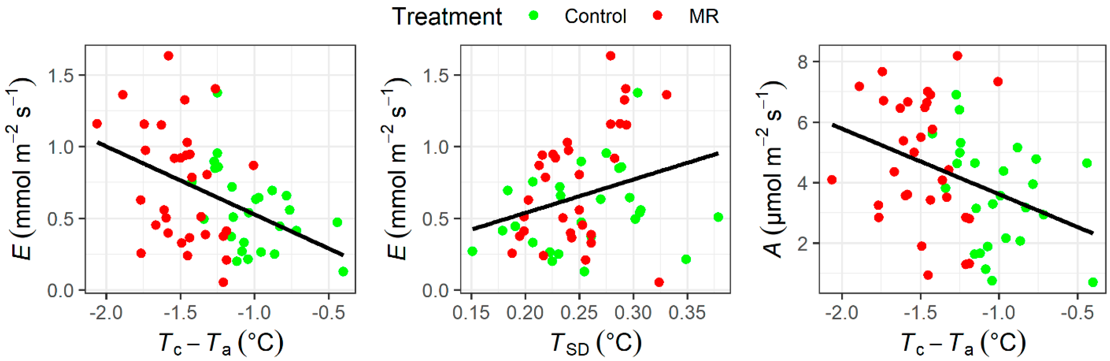
3.5. Tree Physiology and Relationships with Thermal Indices and NBHIs

Prior to inoculation, there were no significant differences between the three physiological variables and values for gs; A and E varied by ≤5% between treatments. In contrast, at 9 DAI all three physiological variables significantly differed (p < 0.05) between treatments. Mean values of these variables for MR plants exceeded those of control plants by 38% for gs (74.8 vs. 54.4 mmol m−2 s−1), 33% for E (0.743 vs. 0.557 mmol m−2 s−1) and 32% for A (4.74 vs. 3.59 µmol m−2 s−1). The linear regressions of these three variables against the 83 NBHIs and thermal indices detected only five relationships that were significant, that all included one of the two thermal indices. For all three physiological variables, TcTa was the strongest significant predictor (Figure 7) which was negatively correlated with E (p = 0.0006; R2 = 0.19), gs (p = 0.0006; R2 = 0.19) and A (p = 0.005; R2 = 0.14). There were also significant positive relationships between TSD and both E (p = 0.03; R2 = 0.08) and gs (p = 0.03; R2 = 0.08) (Figure 7).

4. Discussion

This study highlighted the utility of thermal and VNIR hyperspectral close-range imagery for detection of myrtle rust on pōhutukawa, which is an iconic species under threat from the disease in New Zealand. Using the combined dataset, model performance, as described by the F1 score, ranged from excellent between 3–6 DAI to outstanding (i.e., F1 score > 0.9) from 7–14 DAI. Recent research has successfully used thermal imagery and leaf-level hyperspectral data from a hand held spectroradiometer to detect myrtle rust on rose apple, which is one of the most susceptible hosts of the disease [27]. Findings from the study presented here are consistent with this previous research and extend this approach to a more important target species. The collection of canopy-level imagery, rather than leaf-level hyperspectral data, as used in the previous study [27], allows more direct comparison of model performance with the canopy-level thermal imagery. The collection of this canopy-level hyperspectral imagery is also an important step towards scaling up the detection model using a camera that is often used for acquisition of canopy-level hyperspectral data from a UAV.
This study also demonstrates that robust canopy-level hyperspectral data can be collected under artificial lights. In contrast to outside acquisitions, that rely on clear sky conditions, this novel methodology allows rapid crown level changes in NBHIs resulting from pathogen infection to be characterised at a fine temporal scale. Use of such a method is particularly useful when the pre-visual window for detection is relatively narrow as was the case in this study. The set-up used here does not require the geometric or atmospheric corrections typically necessary for UAV-based captures. On the other hand, achieving uniform illumination of heterogeneous targets such as whole plants using artificial lights is quite challenging.
Hyperspectral indices were found to be more effective than thermal indices for pre-visual detection of infection. As the scanned plants comprised a far greater proportion of older resistant leaves than emerging susceptible leaves, the detected changes mostly reflected shifts in this asymptomatic mature leaf cohort. Pre-visual differences in hyperspectral indices were evident from as early as 3 DAI and by 4 DAI there were widespread differences in xanthophyll indices, the blue band, disease indices and water indices. Within these groupings, the pre-visual indices that were most significantly different between treatments, included, respectively, PRI528, BF1, HI and fWBI.
Normalised canopy temperature was the most useful variable for early disease detection and TcTa showed marked reductions in response to infection from 5 DAI onwards. Following energy balance theory, lower leaf temperature results from increased transpiration which is in turn a result of higher stomatal conductance [41] and observed changes in all these three variables conformed to this theory. Austropuccinia psidii is a biotrophic pathogen [42] and as with other rusts it is likely that these physiological changes were the result of pustules rupturing the cuticle [43]. However, it is also worth noting that the physiological and thermal response of plants to infection also varies according to the infection stage. Development by biotrophic pathogens during later stages is characterised by an increase in the proportion of necrotic tissue which results in reductions in transpiration and increases in leaf temperature [43].
There was strong similarity between results reported here and those from the previous experiment that used hyperspectral and thermal indices to detect myrtle rust on rose apple [27]. Hyperspectral indices derived from symptomless older leaves were the most useful indices for pre-visual detection of myrtle rust on rose apple, while thermal indices were the most effective for later detection immediately before symptom expression and in post-symptomatic plants. As data were collected from a spectroradiometer, indices were derived from both the VNIR (400–1000 nm) and shortwave infrared (SWIR; 1000–2500 nm) ranges within this previous experiment. The most important pre-visual hyperspectral indices derived from the VNIR range on the asymptomatic older leaves were almost identical to those identified in the current study and included PRI528, BF1, HI and WBI [27]. Within the SWIR range, four water indices (Ratio975; NDWI1; SRWI, SRWI2) exhibited strong significant treatment differences two and three days before symptoms appeared, which preceded the differences in WBI, WI and fWBI, extracted from the VNIR range, that occurred the day before symptoms [27].
The key indices used here were also well aligned with previous studies that have used hyperspectral and thermal imagery for pre-visual and early detection of stress. Many studies have shown that the Photochemical Reflectance Index (PRI) is a useful pre-visual indicator of stress [44,45,46] and PRI has been previously used for both early disease detection [47,48] and characterisation of disease severity [49]. Indices derived from the blue part of the spectrum often feature prominently in pre-visual detection studies. Chlorophyll has high absorption in this range [50] and consequently many indices that include wavelengths in the blue region (e.g., NPQI, BGI2) are proxies for degradation of chlorophyll [51,52,53] which is a likely impact of infection by A. psidii [27]. Water stress is a common outcome from disease infection [54] and a range of water indices have proven useful for detection of disease [55,56].
In studies where it has been measured, normalised canopy temperature, as expressed through indices such as TcTa or crop water stress index (CSWI), is frequently an important pre-visual and early indicator of disease [25,26,48]. In contrast to our study, increased canopy temperature is often associated with increased disease severity as previous research has often studied pathogens that cause early reductions in stomatal conductance and transpiration [25,26,47,48]. Consistent with our findings normalised canopy temperature was found to detect almond red leaf blotch later than hyperspectral indices [48]. However, research also shows canopy temperature to be an effective early detector of infection by Xylella fastidiosa [25] and Verticillium wilt [26,47] on olive trees and TcTa was the most effective early discriminator of holm oak decline [21]. The relative efficacy of hyperspectral and thermal imagery depends on the physiological response induced by pathogen infection which likely accounts for this variation [48]. A potential issue when working with thermal data is the separation of temperature and emissivity. While there are emissivity differences between healthy and severely stressed vegetation, differences do not usually occur during the early stress stages examined in this study [57]. As a consequence it was assumed that use of a single emissivity value did not negatively influence the results.
Despite the small sample size the presented results are likely to be robust as a thorough cross validation method was used and there was considerable alignment between predictors identified here and in the earlier study on rose apple [27]. As found previously [25,26,47,48], results reinforced the utility of collecting both thermal and hyperspectral imagery. The use of both hyperspectral and thermal indices provided significant synergies in model performance and importantly, bridged the pre-visual with the early detection period. Ideally, hyperspectral imagery should be collected from a camera that captures the full VNIR/SWIR range as many water indices previously shown to be useful in pre-visual detection of myrtle rust occur within the SWIR range [27]. Previous research has also highlighted the utility of SWIR indices for pre-visual and early detection of disease [21].
Detection of myrtle rust on pōhutukawa is likely to be useful within a nursery setting or for biosecurity purposes in areas where there are important amenity trees or trees of significant cultural and ecological value. As nursery settings are relatively controlled environments, these could provide an opportunity to scale up and fine tune the described methods and examine if they are sufficiently accurate and cost effective for disease detection at a larger scale. Within field settings, previous research has developed a deep learning algorithm using regional aerial RGB imagery that can detect pōhutukawa with high accuracy [58]. The resulting boundaries from this detection algorithm could be used to identify pōhutukawa within aerial acquisitions of thermal and hyperspectral imagery.
Acqusitions of thermal and hyperspectral imagery from UAV or fixed wing aircraft will provide the most appropriate spatial resolution for detection of myrtle rust in pōhutukawa within field settings. Almost all field grown pōhutukawa have a canopy radius exceeding 1.5 m [58] which is most aligned to UAV data collection, where the possible resolutions of 15 cm for thermal imagery [59] and 5 cm for hyperspectral imagery [49,59], enables collection of many pixels per tree. Most VNIR cameras that have been developed for UAVs are less than 5 kg [60]. However, SWIR cameras usually are substantially heavier, as are integrated cameras that can obtain imagery across the VNIR/SWIR range [60] and thus captures across the useful SWIR range will likely need heavy lift UAVs. Data acquisition from a fixed wing aircraft flown at a low altitude could also provide adequate resolution hyperspectral and thermal imagery and it is possible to collect these data at resolutions as fine as 30 cm [60,61]. Although there are a number of satellite platforms that collect thermal and hyperspectral imagery these typically acquire data at a spatial resolution of 30 m for hyperspectral imagery [60] and 60–2000 m for thermal imagery [62], which is too coarse for identification of disease on individual tree canopies.
Scaling up is often complex due to a number of variables that influence the response of hyperspectral and thermal imagery, including canopy structure, sun-sensor geometry, atmospheric conditions and changing environmental conditions [63,64]. The CWSI has been widely adopted as a method of normalising thermal imagery to changing environmental conditions and methods for determining this index have been documented [20]. Radiative transfer models that can account for variability in canopy architecture and image acquisition conditions can be used to accurately simulate canopy thermal properties [65] and describe plant traits useful for predicting disease from hyperspectral imagery [49]. Although scaling up has challenges, a number of studies have successfully detected disease during pre-visual or early stages at broad scales using thermal and hyperspectral imagery [21,25,47,48] demonstrating that robust acquisition and processing pipelines can be developed.

5. Conclusions

Pōhutukawa plants that were inoculated with A. psidii showed the first symptoms by 3 DAI, with all plants displaying symptoms by 8 DAI. Indices extracted from regular captures of plant level thermal and hyperspectral imagery were able to pre-visually distinguish between infected and control plants with considerable accuracy. The NBHIs were most effective at pre-visually classifying treatments and models developed between 3 and 6 DAI had excellent discriminatory power. The normalised canopy temperature, TcTa, which was derived from the thermal imagery was more effective than NBHIs at classifying treatments from 7–14 DAI. There were synergies when indices derived from hyperspectral and thermal imagery were combined, and models using a combination of indices, had excellent classification from 3–6 DAI (F1 score range: 0.81–0.85) and outstanding classification from 7–14 DAI (F1 score range: 0.92–0.93). Further research should extend this method to a nursery setting and examine the potential of thermal and hyperspectral imagery for detecting myrtle rust on field grown Myrtaceae.

Author Contributions

Conceptualization, M.S.W., H.J.C.E. and M.B.; methodology, M.S.W., H.J.C.E., M.B., R.M., W.Y.; E.M. and K.D.; software, Z.H. and H.B., formal analysis, M.S.W.; investigation, M.S.W., H.J.C.E., M.B., R.M., D.P., W.Y., E.M., M.Z., K.D., K.W., Z.H., S.F. and H.B; resources, H.J.C.E., M.B., R.M., D.P. and W.Y.; data curation, H.J.C.E., M.B., R.M., D.P., W.Y., Z.H. and H.B.; writing—original draft preparation, M.S.W. and M.B.; writing—review and editing, M.S.W., H.J.C.E., M.B., R.M., D.P., W.Y., E.M., M.Z., K.D., K.W., Z.H., S.F. and H.B.; visualization, M.S.W. and H.J.C.E.; supervision, H.J.C.E., M.S.W., H.J.C.E., M.B., R.M. and S.F.; project administration, H.J.C.E.; funding acquisition, H.J.C.E., M.S.W., S.F. and M.B. All authors have read and agreed to the published version of the manuscript.

Funding

This project was funded through Scion SSIF funding and the Ministry of Business, Innovation and Employment (MBIE) programme grant numbers C04X2101 (Seeing the forest for the trees: transforming tree phenotyping for future forests) and C09X1806 (Beyond myrtle rust: Towards ecosystem resilience).

Data Availability Statement

The data presented in this study are available on reasonable request from the corresponding author.

Acknowledgments

We thank Thomas Rosenburg, Catherine Banham, Hannah Thompson, and Andrew Pugh for assistance with disease assessments and maintaining plants during the experiment. We are also grateful to Anita Wylie, Matt Dunn, and Scion nursery staff for maintaining plants prior to the experiment and Peter Massam for setting up equipment and getting the dark room ready. We also thank Tara Strand for allocating SSIF funds to this project and Elizaveta Graevskaya for help in arranging SSIF funding for the project. We are grateful to the anonymous reviewers for comments that greatly improved the manuscript. Scion’s standard practice is to source indigenous trees and materials with full knowledge and permission of mana whenua (the iwi/tribe or hapū/sub-tribe who have customary authority over land) to carry out the science research. In this case, pōhutukawa seedlings were sourced from a nursery that could not determine the exact source of the trees. Scion’s Te Ao Māori Research Group endeavoured to ensure that the trees were cared for in an appropriate manner according to tikanga Māori (Māori customary practice). Specifically, Selwyn Insley (Pou Hononga Māori Partnerships Lead) delivered karakia (prayer) before the research began, after infection, and upon disposal of the heavily infected pōhutukawa. All appropriate cultural procedures were adhered to.

Conflicts of Interest

The authors declare no conflicts of interest.

Appendix A

Table A1. Thermal and narrow-band hyperspectral indices (NBHIs) that were used in analyses.
IndicesEquationRef.
Thermal indices
Normalised canopy temperatureTcTa[66]
Standard deviation normalised temp.TSD = std dev (TcTa)[66]
Xanthophyll indices
Photochemical Refl. Index (570) P R I 570 = ( R 570 R 531 ) / ( R 570 + R 531 ) [67]
Photochemical Refl. Index (515) P R I 515 = ( R 515 R 531 ) / ( R 515 + R 531 ) [68]
Photochemical Refl. Index (528) P R I 528 = ( R 528 R 567 ) / ( R 528 + R 567 ) [67]
Photochemical Refl. Index (550) P R I 550 = ( R 550 R 531 ) / ( R 550 + R 531 ) [67]
Photochemical Refl. Index m1 P R I m 1 = ( R 512 R 531 ) / ( R 512 + R 531 ) [68]
Photochemical Refl. Index m2 P R I m 2 = ( R 600 R 531 ) / ( R 600 + R 531 ) [67]
Photochemical Refl. Index m3 P R I m 3 = ( R 670 R 531 ) / ( R 670 + R 531 ) [67]
Photochemical Refl. Index m4 P R I m 4 = ( R 570 R 531 R 670 ) / ( R 570 + R 531 + R 670 ) [68]
Normalized Photoch. Refl. Index P R I n = P R I 570 / [ R D V I · ( R 700 / R 670 ) ] [69]
Ratio of PRI to Simple Ratio D R I   P R I = P R I 570 / ( R 800 / R 670 ) [70]
Carotenoid/Chlorophyll Ratio Index P R I · C I = ( R 570 R 530 ) / ( R 570 + R 530 ) · ( ( R 760 / R 700 ) 1 ) [71]
R/G/B indices
Redness Index R = R 700 / R 670 [72]
Greenness Index G = R 570 / R 670 [47]
Greenness Index 2 G I = R 554 / R 677 [73]
Blue Index B = R 450 / R 490 [47]
Blue/green indices B G I 1 = R 400 / R 550 [73]
B G I 2 = R 450 / R 550 [73]
Blue/red indices B R I 1 = R 400 / R 690 [74]
B R I 2 = R 450 / R 690 [74]
BF1 B F 1 = R 400 / R 410 [25]
BF2 B F 2 = R 400 / R 420 [25]
BF3 B F 3 = R 400 / R 430 [25]
BF4 B F 4 = R 400 / R 440 [25]
BF5 B F 5 = R 400 / R 450 [25]
Red/green index R G I = R 690 / R 550 [73]
Ratio Analysis of Reflectance Spectra R A R S = R 746 / R 513 [75]
Lichtenthaler indices L I C 1 = R 800 R 680 / R 800 + R 680 [76]
L I C 2 = R 440 / R 690 [76]
L I C 3 = R 440 / R 740 [76]
Plant disease indices
Cercospora leaf spot index C L S = R 698 R 570 R 698 + R 570 R 734 [22]
Healthy-index H I = R 534 R 698 R 534 + R 698 1 2 · R 704 [22]
Powdery mildew index P M I = R 520 R 584 R 520 + R 584 + R 724 [22]
Sugar beet rust–index S B R I = R 570 R 513 R 570 + R 513 + 1 2 · R 704 [22]
Water Indices
Floating position Water Band index f W B I = R 900 / m i n R 930 R 980 [77]
Water Band Index W B I = R 970 / R 900 [78]
Water Index W I = R 900 / R 970 [79]
Curvature index
Curvature index C U R = R 675   R 690 / R 683 2 [80]
Structural indices
Normalized Difference Veg. Index N D V I = ( R 800 R 670 ) / ( R 800 + R 670 ) [81]
Renormalized Difference Veg. Index R D V I = ( R 800 R 670 ) / ( R 800 + R 670 ) [82]
Optimized Soil-Adjusted Veg. Index O S A V I = ( 1 + 0.16 · ( R 800 R 670 ) / ( R 800 + R 670 + 0.16 ) ) [83]
Modified Soil-Adjusted Vegetation Index M S A V I = 2 · R 800 + 1 ( 2 · R 800 + 1 ) 2 8 ( R 800 R 670 ) 2 [84]
Triangular Vegetation Index T V I = 0.5 · [ 120 · R 750 R 550 200 · R 670 R 550 ] [85]
Modified Triangular Veg. Index 1 M T V I 1 = 1.2 [ 1.2 R 800 R 550 2.5 R 670 R 550 ] [86]
Modified Triangular Veg. Index 2 M T V I 2 = 1.5 1.2 R 800 R 550 2.5 R 670 R 550 ( 2 R 800 + 1 ) 2 6 R 800 5 R 670 0.5 [86]
Chlorophyll Abs. Reflectance Index C A R I = R 700 R 670 0.2 R 700 R 550     [87]
Modified Chlorophyll Abs. Index M C A R I = R 700 R 670 0.2 R 700 R 550 · ( R 700 / R 670 ) [86]
Modified Chlorophyll Abs. Index 1 M C A R I 1 = 1.2 2.5 R 800 R 670 1.3 R 800 R 550 [86]
Modified Chlorophyll Abs. Index 2 M C A R I 2 = 1.5 2.5 R 800 R 670 1.3 R 800 R 550 ( 2 R 800 + 1 ) 2 6 R 800 5 R 670 0.5 [86]
Modified Chlorophyll Abs. Index 3 M C A R I 3 = R 750 R 705 0.2 R 750 R 550 · ( R 750 / R 705 ) [88]
Simple Ratio S R = R 800 / R 670 [89]
Modified Simple Ratio M S R = R 800 / R 670 1 ( R 800 / R 670 ) 0.5 + 1 [90]
Enhanced Vegetation Index E V I = 2.5 · R 800 R 670 / R 800 + 6 · R 670 7.5 · R 800 + 1 [91]
Pigment indices
Vogelmann indices V O G 1 = R 740 / R 720 [92]
V O G 2 = ( R 734 R 747 ) / ( R 715 + R 726 ) [92]
V O G 3 = ( R 734 R 747 ) / ( R 715 + R 720 ) [92]
Gitelson & Merzlyak indices G M 1 = R 750 / R 550 [53]
G M 2 = R 750 / R 700 [53]
G M 4 = R 750 / R 555 [93]
Transformed Chlorophyll Absorption in Reflectance Index T C A R I = 3 · [ R 700 R 670 0.2 · R 700 R 550 R 700 R 670 ] [94]
TCARI/OSAVI T C A R I O S A V I [94]
Chlorophyll Index Red Edge C I = R 750 / R 710 [94]
Simple Ratio Pigment Index S R P I = R 430 / R 680 [51,95]
Normalized Phaeophytinization Index N P Q I = ( R 415 R 435 ) / ( R 415 + R 435 ) [51,95]
Normalized Pigments Index N P C I = ( R 680 R 430 ) / ( R 680 + R 430 ) [95]
Carter indices C T R 1 = R 695 / R 420 [96]
C A R = R 695 / R 760 [97]
Reflectance band ratio indices D C a b C x c = R 672 / ( R 550 · R 708 ) [98]
D N I R C a b C x c = R 860 / ( R 550 · R 708 ) [98]
Structure-Insensitive Pigment Index S I P I = ( R 800 R 445 ) / ( R 800 R 680 ) [95]
Carotenoid Reflectance Indices C R I 550 = 1 / R 510 1 / R 550 [99,100]
C R I 700 = 1 / R 510 1 / R 700 [99]
C R I 550   515 = 1 / R 515 1 / R 550 [99]
C R I 700   515 = 1 / R 515 1 / R 700 [99]
R N I R · C R I 550 = ( 1 / R 510 1 / R 550 ) · R 770 [99,100]
R N I R · C R I 700 = ( 1 / R 510 1 / R 700 ) · R 770 [99,100]
Plant Senescing Reflectance Index P S R I = ( R 680 R 500 ) / R 750 [101]
Pigment Specific Simple Ratio Chlorophyll a P S S R a = R 800 / R 675 [102]
Pigment Spec. Simple Ratio Chl. b P S S R b = R 800 / R 650 [102]
Pigment Specific Simple Ratio Carotenoid P S S R c = R 800 / R 500 [102]
Pigment Specific Normalized Difference P S N D c = ( R 800 R 470 ) / ( R 800 + R 470 ) [102]
Reciprocal reflectance R R = 1 / R 700 [103]
Table A2. One-way analysis of variance between treatments for hyperspectral and thermal indices used in the study over the eight infection stages. The p values are colour-coded according to the strength of the significance. Red shaded cells indicate a highly significant effect, orange cells indicate marginal significance, and yellow and green shaded cells indicate moderate to strong insignificance, respectively. Indices are sorted according to their type and follow the order shown in Table A1.
Index TypeVariableDays after Inoculation
Pre-Treat34567814
Thermal indicesTcTa0.93390.99730.01510.02020.00018.0 × 10−101.5 × 10−104.9 × 10⁻¹²
TSD0.73410.74620.75470.12670.50070.04380.77400.4121
Xanthophyll PRI5700.16960.33320.87860.44860.63890.92580.66620.0001
indicesPRI5150.67130.98500.77610.93590.81900.79720.88240.9736
PRI5280.11640.01050.02490.01610.00450.01590.28690.0632
PRI5500.74380.82010.86780.78750.57770.76700.46210.0119
PRIm10.53210.96170.85830.85230.89470.69650.66620.7227
PRIm20.80270.53390.50100.99190.95160.75480.70280.0016
PRIm30.41720.97600.41420.76220.78770.95190.89880.1006
PRIm40.25920.60610.42350.52540.98720.97920.88630.4564
PRIn0.14950.31960.24000.50440.61550.94950.66154.2 × 10−5
DRI PRI0.11200.13630.06590.27060.33670.91110.31303.3 × 10−5
PRI CI0.28100.47280.85240.30620.78500.90600.63400.0252
R/G/B IndicesR0.26910.65160.02210.55730.78840.69370.40570.3709
G0.35970.93020.46490.68740.82230.96470.90660.4573
GI0.42790.92130.84930.79290.56560.76460.72600.3613
B0.35260.45890.00270.01560.52870.20280.60330.0084
BGI10.80360.57670.01140.40780.89600.44310.74730.0561
BGI20.65550.79160.28650.47790.99070.80350.88280.0849
BRI10.87120.73110.03300.44180.55250.60600.89890.0245
BRI20.69720.90570.94000.47290.37430.80330.28860.0078
BF10.94670.13140.00010.37410.44190.12470.21080.0128
BF20.97290.42070.00100.34130.86760.12490.64320.0309
BF30.99670.38560.00180.33170.54230.28560.72650.0588
BF40.89100.40000.00200.28610.69010.26050.59670.0458
BF50.95840.56720.00190.57330.65330.39330.67900.1121
RGI0.71440.61740.12880.78000.24760.53550.32520.4593
RARS0.62150.81750.19980.77590.52640.60260.52250.8905
LIC10.99350.82170.32020.93490.60210.65640.92790.8995
LIC20.65160.61190.86300.94250.33140.54780.24420.0339
LIC30.84520.99570.98650.86790.71820.87870.56470.2464
Plant diseaseCLS0.90840.59160.10200.26500.55840.30570.12840.0038
indicesHI0.21380.34110.00330.55090.18790.39930.11740.1151
PMI0.93850.58720.68850.17530.62170.34060.26440.0961
SBRI0.32960.63730.61800.75000.55320.66950.79720.1207
Water indicesfWBI0.65270.28580.00270.65180.34170.90340.11090.1139
WBI0.95720.30240.00410.23410.67960.03480.12910.4479
WI0.95670.29520.00390.23000.67220.03400.12730.4415
Curvature indexCUR0.14170.85520.46860.82270.04790.17690.41350.2775
Index typeVariableDays after inoculation
Pre-treat34567814
StructuralNDVI0.96980.86640.18130.93120.91710.92390.89420.7090
IndicesRDVI0.96710.79380.67540.29420.82200.47840.22380.0020
OSAVI0.92560.75270.28830.40710.85180.61100.42680.0307
MSAVI0.85010.75990.31390.42040.99370.73760.55170.0291
TVI0.84540.86320.96360.31200.93350.53320.26830.0031
MTVI10.79780.86140.92230.32580.84730.49900.22810.0020
MTVI20.54110.82220.29690.47580.97620.73790.46830.0342
CARI0.23920.67300.41070.98090.75830.87780.91670.4113
MCARI0.22410.62620.19320.84800.74740.83980.74880.7026
MCARI10.79780.86140.92230.32580.84730.49900.22810.0020
MCARI20.54110.82220.29690.47580.97620.73790.46830.0342
MCARI30.43490.86730.83780.53700.98430.72560.44630.1168
SR0.97450.91730.12010.78870.87550.85290.70280.5369
MSR0.97370.97530.13250.82570.93060.91240.75170.5790
EVI0.83830.78870.89610.33330.99870.68440.37900.0030
Pigment indicesVOG10.51780.68160.58400.70910.49730.53560.78140.9248
VOG20.56440.49780.30410.51410.35580.36670.75600.8244
VOG30.57050.50470.32540.53100.36780.38280.74560.8214
GM10.52320.84570.32510.87660.73830.84310.65650.9276
GM20.35310.87880.90080.92240.96190.95670.94950.8588
GM40.51390.85360.33660.87260.75110.82400.67820.9259
TCARI0.29160.78810.66870.91700.83860.93810.95170.3950
TCARI/OSAVI0.28560.75140.73350.99510.81270.87620.97810.5465
CI10.43460.89190.82060.96020.76720.88400.95080.9723
SRPI0.56240.98340.03010.57350.44670.86620.67570.0166
NPQI0.54000.77470.06820.59940.22530.17060.92080.6934
NPCI0.53490.99040.03080.64670.39820.87100.67890.0193
CTR10.38980.82250.64540.96150.35690.79550.52740.0895
CAR0.24710.60850.78770.74020.75320.74480.75070.9543
DCabCxc0.40160.82450.97260.67210.70130.70630.51850.2347
DNIRCabCxc0.60540.65450.38160.59010.60130.61870.43150.2525
SIPI0.44440.82750.03830.40060.39020.98220.65380.0054
CRI5500.90780.97250.55310.60460.92430.72010.25420.2296
CRI7000.96020.80920.16350.49660.73190.58700.14780.2726
CRI550 5150.71290.88530.38130.58310.69050.58690.31720.1489
CRI700 5150.91130.67490.07260.45980.52300.46120.15970.2026
RNIR CRI5500.94170.85060.38180.99910.95230.90220.41030.4427
RNIR CRI7000.89650.85540.06740.78580.70200.70040.22220.4876
PSRI0.39470.89870.94640.98150.08380.22450.07030.0101
PSSRa0.99990.91730.15180.78810.99740.98510.77580.5944
PSSRb0.74170.91290.12740.84050.78110.79510.58790.5271
PSSRc0.75630.93710.22290.91270.80680.89230.55290.6924
PSNDc0.92070.87000.41060.90460.98410.80720.76080.4588
RR0.41560.95810.94060.64720.88380.79130.56920.0741
Figure A1. Progression of myrtle rust on an inoculated pōhutukawa plant showing changes in RGB imagery and normalised canopy temperature (Tc − Ta), derived from thermal imagery for the pre-inoculation stage (left panels) and for 6 days (middle panels) and 14 days (right panels) after inoculation. The first two rows show changes for the whole plant, while the third and fourth row show changes for a part of the plant (red box, second row) that includes older leaves (dark green) that do not show visual symptoms and younger (light green) leaves that are susceptible to infection and show visual symptoms. The image clearly shows that despite being resistant to infection, the older leaves still show reduced values for Tc − Ta as the disease progresses.
Remotesensing 16 01050 g0a1

References

  1. Wingfield, M.J.; Slippers, B.; Wingfield, B.D.; Barnes, I. The unified framework for biological invasions: A forest fungal pathogen perspective. Biol. Invasions 2017, 19, 3201–3214. [Google Scholar] [CrossRef]
  2. Beenken, L. Austropuccinia: A new genus name for the myrtle rust Puccinia psidii placed within the redefined family Sphaerophragmiaceae (Pucciniales). Phytotaxa 2017, 297, 53–61. [Google Scholar] [CrossRef]
  3. Stewart, J.E.; Ross-Davis, A.L.; Graça, R.N.; Alfenas, A.C.; Peever, T.L.; Hanna, J.W.; Uchida, J.Y.; Hauff, R.D.; Kadooka, C.Y.; Kim, M.S.; et al. Genetic diversity of the myrtle rust pathogen (Austropuccinia psidii) in the Americas and Hawaii: Global implications for invasive threat assessments. For. Pathol. 2017, 48, e12378. [Google Scholar] [CrossRef]
  4. Glen, M.; Alfenas, A.C.; Zauza, E.A.V.; Wingfield, M.J.; Mohammed, C. Puccinia psidii: A threat to the Australian environment and economy—A review. Australas. Plant Pathol. 2007, 36, 1–16. [Google Scholar] [CrossRef]
  5. Carnegie, A.J.; Pegg, G.S. Lessons from the Incursion of Myrtle Rust in Australia. Annu. Rev. Phytopathol. 2018, 56, 457–478. [Google Scholar] [CrossRef]
  6. Berthon, K.A.; Fernandez Winzer, L.; Sandhu, K.; Cuddy, W.; Manea, A.; Carnegie, A.J.; Leishman, M.R. Endangered species face an extra threat: Susceptibility to the invasive pathogen Austropuccinia psidii (myrtle rust) in Australia. Australas. Plant Pathol. 2019, 48, 385–393. [Google Scholar] [CrossRef]
  7. Soewarto, J.; Giblin, F.; Carnegie, A.J. Austropuccinia psidii (Myrtle Rust) Global Host List, Version 4; Australian Network for Plant Conservation: Canberra, ACT, Australia, 2019. [Google Scholar]
  8. Almeida, R.F.; Machado, P.S.; Damacena, M.B.; Santos, S.A.; Guimarães, L.M.S.; Klopfenstein, N.B.; Alfenas, A.C. A new, highly aggressive race of Austropuccinia psidii infects a widely planted, myrtle rust-resistant, eucalypt genotype in Brazil. For. Pathol. 2021, 51, e12679. [Google Scholar] [CrossRef]
  9. Fensham, R.J.; Radford-Smith, J. Unprecedented extinction of tree species by fungal disease. Biol. Conserv. 2021, 261, 109276. [Google Scholar] [CrossRef]
  10. Heim, R.H.J.; Wright, I.J.; Allen, A.P.; Geedicke, I.; Oldeland, J. Developing a spectral disease index for myrtle rust (Austropuccinia psidii). Plant Pathol. 2019, 68, 738–745. [Google Scholar] [CrossRef]
  11. Soewarto, J.; Carriconde, F.; Hugot, N.; Bocs, S.; Hamelin, C.; Maggia, L.; Klopfenstein, N.B. Impact of Austropuccinia psidii in New Caledonia, a biodiversity hotspot. For. Pathol. 2018, 48, e12402. [Google Scholar] [CrossRef]
  12. Sutherland, R.; Soewarto, J.; Beresford, R.; Ganley, B. Monitoring Austropuccinia psidii (myrtle rust) on New Zealand Myrtaceae in native forest. N. Z. J. Ecol. 2020, 44, 1–5. [Google Scholar] [CrossRef]
  13. Soewarto, J.; Somchit, C.; du Plessis, E.; Barnes, I.; Granados, G.M.; Wingfield, M.J.; Shuey, L.; Bartlett, M.; Fraser, S.; Scott, P.; et al. Susceptibility of native New Zealand Myrtaceae to the South African strain of Austropuccinia psidii: A biosecurity threat. Plant Pathol. 2021, 70, 667–675. [Google Scholar] [CrossRef]
  14. Beresford, R.M.; Shuey, L.S.; Pegg, G.S. Symptom development and latent period of Austropuccinia psidii (myrtle rust) in relation to host species, temperature, and ontogenic resistance. Plant Pathol. 2020, 69, 484–494. [Google Scholar] [CrossRef]
  15. Baskarathevan, J.; Taylor, R.K.; Ho, W.; McDougal, R.L.; Shivas, R.G.; Alexander, B.J.R. Real-Time PCR Assays for the Detection of Puccinia psidii. Plant Dis. 2016, 100, 617–624. [Google Scholar] [CrossRef]
  16. Bini, A.P.; Quecine, M.C.; da Silva, T.M.; Silva, L.D.; Labate, C.A. Development of a quantitative real-time PCR assay using SYBR Green for early detection and quantification of Austropuccinia psidii in Eucalyptus grandis. Eur. J. Plant Pathol. 2017, 150, 735–746. [Google Scholar] [CrossRef]
  17. Carnegie, A.J.; Cooper, K. Emergency response to the incursion of an exotic myrtaceous rust in Australia. Australas. Plant Pathol. 2011, 40, 346–359. [Google Scholar] [CrossRef]
  18. Langrell, S.R.H.; Glen, M.; Alfenas, A.C. Molecular diagnosis of Puccinia psidii (guava rust)—A quarantine threat to Australian eucalypt and Myrtaceae biodiversity. Plant Pathol. 2008, 57, 687–701. [Google Scholar] [CrossRef]
  19. Roux, J.; Greyling, I.; Coutinho, T.A.; Verleur, M.; Wingfield, M.J. The Myrtle rust pathogen, Puccinia psidii, discovered in Africa. IMA Fungus 2013, 4, 155–159. [Google Scholar] [CrossRef]
  20. Hernández-Clemente, R.; Hornero, A.; Mottus, M.; Penuelas, J.; González-Dugo, V.; Jiménez, J.C.; Suárez, L.; Alonso, L.; Zarco-Tejada, P.J. Early Diagnosis of Vegetation Health From High-Resolution Hyperspectral and Thermal Imagery: Lessons Learned From Empirical Relationships and Radiative Transfer Modelling. Curr. For. Rep. 2019, 5, 169–183. [Google Scholar] [CrossRef]
  21. Hornero, A.; Zarco-Tejada, P.J.; Quero, J.L.; North, P.R.J.; Ruiz-Gómez, F.J.; Sánchez-Cuesta, R.; Hernandez-Clemente, R. Modelling hyperspectral-and thermal-based plant traits for the early detection of Phytophthora-induced symptoms in oak decline. Remote Sens. Environ. 2021, 263, 112570. [Google Scholar] [CrossRef]
  22. Mahlein, A.K.; Rumpf, T.; Welke, P.; Dehne, H.W.; Plümer, L.; Steiner, U.; Oerke, E.C. Development of spectral indices for detecting and identifying plant diseases. Remote Sens. Environ. 2013, 128, 21–30. [Google Scholar] [CrossRef]
  23. Poblete, T.; Camino, C.; Beck, P.S.A.; Hornero, A.; Kattenborn, T.; Saponari, M.; Boscia, D.; Navas-Cortes, J.A.; Zarco-Tejada, P.J. Detection of Xylella fastidiosa infection symptoms with airborne multispectral and thermal imagery: Assessing bandset reduction performance from hyperspectral analysis. ISPRS J. Photogramm. Remote Sens. 2020, 162, 27–40. [Google Scholar] [CrossRef]
  24. Tian, L.; Xue, B.; Wang, Z.; Li, D.; Yao, X.; Cao, Q.; Zhu, Y.; Cao, W.; Cheng, T. Spectroscopic detection of rice leaf blast infection from asymptomatic to mild stages with integrated machine learning and feature selection. Remote Sens. Environ. 2021, 257, 112350. [Google Scholar] [CrossRef]
  25. Zarco-Tejada, P.J.; Camino, C.; Beck, P.S.A.; Calderon, R.; Hornero, A.; Hernández-Clemente, R.; Kattenborn, T.; Montes-Borrego, M.; Susca, L.; Morelli, M. Previsual symptoms of Xylella fastidiosa infection revealed in spectral plant-trait alterations. Nat. Plants 2018, 4, 432–439. [Google Scholar] [CrossRef]
  26. Calderón, R.; Navas-Cortés, J.A.; Zarco-Tejada, P.J. Early detection and quantification of Verticillium wilt in olive using hyperspectral and thermal imagery over large areas. Remote Sens. 2015, 7, 5584–5610. [Google Scholar] [CrossRef]
  27. Watt, M.S.; Bartlett, M.; Soewarto, J.; de Silva, D.; Estarija, H.J.C.; Massam, P.; Cajes, D.; Yorston, W.; Graevskaya, E.; Dobbie, K. Previsual and early detection of myrtle rust on rose apple using indices derived from thermal imagery and visible-to-short-infrared spectroscopy. Phytopathology 2023, 113, 1405–1416. [Google Scholar] [CrossRef]
  28. Bylsma, R.J.; Clarkson, B.D.; Efford, J.T. Biological flora of New Zealand 14: Metrosideros excelsa, pōhutukawa, New Zealand Christmas tree. N. Z. J. Bot. 2014, 52, 365–385. [Google Scholar] [CrossRef]
  29. Black, A.; Garner, G.; Mark-Shadbolt, M.; Balanovic, J.; MacDonald, E.; Mercier, O.; Wright, J.; Calver, M. Indigenous peoples’ attitudes and social acceptability of invasive species control in New Zealand. Pac. Conserv. Biol. 2021, 28, 481–490. [Google Scholar] [CrossRef]
  30. Teulon, D.A.J.; Alipia, T.T.; Ropata, H.T.; Green, J.M.; Viljanen, S.L.H.; Cromey, M.G.; Arthur, K.; MacDairmid, R.M.; Waipara, N.W.; Marsh, A.T. The threat of myrtle rust to Māori taonga plant species in New Zealand. N. Z. Plant Prot. 2015, 68, 66–75. [Google Scholar]
  31. Dawson, M.; Hobbs, J.; Platt, G.; Rumbal, J. Metrosideros in cultivation: Pōhutukawa. N. Z. Gard. J. 2010, 13, 10–22. [Google Scholar]
  32. Beresford, R.M.; Turner, R.; Tait, A.; Paul, V.; Macara, G.; Yu, Z.D.; Lima, L.; Martin, R. Predicting the climatic risk of myrtle rust during its first year in New Zealand. N. Z. Plant Prot. 2018, 71, 332–347. [Google Scholar] [CrossRef]
  33. Toome-Heller, M.; Ho, W.W.H.; Ganley, R.J.; Elliott, C.E.A.; Quinn, B.; Pearson, H.G.; Alexander, B.J.R. Chasing myrtle rust in New Zealand: Host range and distribution over the first year after invasion. Australas. Plant Pathol. 2020, 49, 221–230. [Google Scholar] [CrossRef]
  34. Ho, W.H.; Baskarathevan, J.; Griffin, R.L.; Quinn, B.D.; Alexander, B.J.R.; Havell, D.; Ward, N.A.; Pathan, A.K. First report of myrtle rust caused by Austropuccinia psidii on Metrosideros kermadecensis on Raoul Island and on M. excelsa in Kerikeri, New Zealand. Plant Dis. 2019, 103, 2128. [Google Scholar] [CrossRef]
  35. Ministry for Primary Industries. Species Infected with Myrtle Rust in New Zealand. 2024. Available online: https://myrtlerust-uat.biosites.mpi.govt.nz/about-myrtle-rust/species-infected-with-myrtle-rust-in-new-zealand/ (accessed on 12 February 2024).
  36. Rasband, W.S. ImageJ; U.S. National Institutes of Health: Bethesda, MD, USA, 2012. Available online: https://imagej.nih.gov/ij/ (accessed on 11 December 2023).
  37. Buddenbaum, H.; Watt, M.S.; Scholten, R.C.; Hill, J. Preprocessing ground-based visible/near infrared imaging spectroscopy data affected by smile effects. Sensors 2019, 19, 1543. [Google Scholar] [CrossRef]
  38. R Core Team. R: A Language and Environment for Statistical Computing; R Foundation for Statistical Computing: Vienna, Austria, 2023; Available online: https://www.R-project.org/ (accessed on 2 February 2024).
  39. Pedregosa, F.; Varoquaux, G.; Gramfort, A.; Michel, V.; Thirion, B.; Grisel, O.; Blondel, M.; Prettenhofer, P.; Weiss, R.; Dubourg, V. Scikit-learn: Machine Learning in Python. J. Mach. Learn. Res. 2011, 12, 2825–2830. [Google Scholar]
  40. Yuan, X.; Chen, S.; Sun, C.; Yuwen, L. A novel early diagnostic framework for chronic diseases with class imbalance. Sci. Rep. 2022, 12, 8614. [Google Scholar] [CrossRef] [PubMed]
  41. Still, C.; Powell, R.; Aubrecht, D.; Kim, Y.; Helliker, B.; Roberts, D.; Richardson, A.D.; Goulden, M. Thermal imaging in plant and ecosystem ecology: Applications and challenges. Ecosphere 2019, 10, e02768. [Google Scholar] [CrossRef]
  42. Chock, M.K. The global threat of Myrtle rust (Austropuccinia psidii): Future prospects for control and breeding resistance in susceptible hosts. Crop Protect. 2020, 136, 105176. [Google Scholar] [CrossRef]
  43. Smith, R.C.G.; Heritage, A.D.; Stapper, M.; Barrs, H.D. Effect of stripe rust (Puccinia striiformis West.) and irrigation on the yield and foliage temperature of wheat. Field Crops Res. 1986, 14, 39–51. [Google Scholar] [CrossRef]
  44. Nichol, C.J.; Rascher, U.; Matsubara, S.; Osmond, B. Assessing photosynthetic efficiency in an experimental mangrove canopy using remote sensing and chlorophyll fluorescence. Trees 2006, 20, 9–15. [Google Scholar] [CrossRef]
  45. Peguero-Pina, J.J.; Morales, F.; Flexas, J.; Gil-Pelegrín, E.; Moya, I. Photochemistry, remotely sensed physiological reflectance index and de-epoxidation state of the xanthophyll cycle in Quercus coccifera under intense drought. Oecologia 2008, 156, 1–11. [Google Scholar] [CrossRef] [PubMed]
  46. Zarco-Tejada, P.J.; Berni, J.A.J.; Suárez, L.; Sepulcre-Cantó, G.; Morales, F.; Miller, J.R. Imaging chlorophyll fluorescence with an airborne narrow-band multispectral camera for vegetation stress detection. Remote Sens. Environ. 2009, 113, 1262–1275. [Google Scholar] [CrossRef]
  47. Calderón, R.; Navas-Cortés, J.A.; Lucena, C.; Zarco-Tejada, P.J. High-resolution airborne hyperspectral and thermal imagery for early detection of Verticillium wilt of olive using fluorescence, temperature and narrow-band spectral indices. Remote Sens. Environ. 2013, 139, 231–245. [Google Scholar] [CrossRef]
  48. López-López, M.; Calderón, R.; González-Dugo, V.; Zarco-Tejada, P.J.; Fereres, E. Early detection and quantification of almond red leaf blotch using high-resolution hyperspectral and thermal imagery. Remote Sens. 2016, 8, 276. [Google Scholar] [CrossRef]
  49. Watt, M.S.; Poblete, T.; de Silva, D.; Estarija, H.J.C.; Hartley, R.J.L.; Leonardo, E.M.C.; Massam, P.; Buddenbaum, H.; Zarco-Tejada, P.J. Prediction of the severity of Dothistroma needle blight in radiata pine using plant based traits and narrow band indices derived from UAV hyperspectral imagery. Agric. For. Meteorol. 2023, 330, 109294. [Google Scholar] [CrossRef]
  50. Lichtenthaler, H.K.; Rinderle, U. The role of chlorophyll fluorescence in the detection of stress conditions in plants. CRC Crit. Rev. Anal. Chem. 1988, 19, S29–S85. [Google Scholar] [CrossRef]
  51. Barnes, J.D.; Balaguer, L.; Manrique, E.; Elvira, S.; Davison, A.W. A reappraisal of the use of DMSO for the extraction and determination of chlorophylls a and b in lichens and higher plants. Environ. Exp. Bot. 1992, 32, 85–100. [Google Scholar] [CrossRef]
  52. Penuelas, J.; Filella, I.; Lloret, P.; Mun Oz, F.; Vilajeliu, M. Reflectance assessment of mite effects on apple trees. Int. J. Remote Sens. 1995, 16, 2727–2733. [Google Scholar] [CrossRef]
  53. Gitelson, A.A.; Merzlyak, M.N. Signature analysis of leaf reflectance spectra: Algorithm development for remote sensing of chlorophyll. J. Plant Physiol. 1996, 148, 494–500. [Google Scholar] [CrossRef]
  54. Oliva, J.; Stenlid, J.; Martinez-Vilalta, J. The effect of fungal pathogens on the water and carbon economy of trees: Implications for drought-induced mortality. New Phytol. 2014, 203, 1028–1035. [Google Scholar] [CrossRef]
  55. Skoneczny, H.; Kubiak, K.; Spiralski, M.; Kotlarz, J.; Mikiciński, A.; Puławska, J. Fire blight disease detection for apple trees: Hyperspectral analysis of healthy, infected and dry leaves. Remote Sens. 2020, 12, 2101. [Google Scholar] [CrossRef]
  56. Kim, S.-R.; Lee, W.-K.; Lim, C.-H.; Kim, M.; Kafatos, M.C.; Lee, S.-H.; Lee, S.-S. Hyperspectral analysis of pine wilt disease to determine an optimal detection index. Forests 2018, 9, 115. [Google Scholar] [CrossRef]
  57. Buddenbaum, H.; Rock, G.; Hill, J.; Werner, W. Measuring stress reactions of beech seedlings with PRI, fluorescence, temperatures and emissivity from VNIR and thermal field imaging spectroscopy. Eur. J. Remote Sens. 2015, 48, 263–282. [Google Scholar] [CrossRef]
  58. Pearse, G.D.; Watt, M.S.; Soewarto, J.; Tan, A.Y.S. Deep learning and phenology enhance large-scale tree species classification in aerial imagery during a biosecurity response. Remote Sens. 2021, 13, 1789. [Google Scholar] [CrossRef]
  59. Duarte, A.; Borralho, N.; Cabral, P.; Caetano, M. Recent advances in forest insect pests and diseases monitoring using UAV-based data: A systematic review. Forests 2022, 13, 911. [Google Scholar] [CrossRef]
  60. Watt, M.S.; Pearse, G.D.; Dash, J.P.; Melia, N.; Leonardo, E.M.C. Application of remote sensing technologies to identify impacts of nutritional deficiencies on forests. ISPRS J. Photogramm. Remote Sens. 2019, 149, 226–241. [Google Scholar] [CrossRef]
  61. Neinavaz, E.; Schlerf, M.; Darvishzadeh, R.; Gerhards, M.; Skidmore, A.K. Thermal infrared remote sensing of vegetation: Current status and perspectives. Int. J. Appl. Earth Obs. Geoinf. 2021, 102, 102415. [Google Scholar] [CrossRef]
  62. Smigaj, M.; Agarwal, A.; Bartholomeus, H.; Decuyper, M.; Elsherif, A.; de Jonge, A.; Kooistra, L. Thermal Infrared Remote Sensing of Stress Responses in Forest Environments: A Review of Developments, Challenges, and Opportunities. Curr. For. Rep. 2024, 10, 56–76. [Google Scholar] [CrossRef]
  63. Asner, G.P. Biophysical and biochemical sources of variability in canopy reflectance. Remote Sens. Environ. 1998, 64, 234–253. [Google Scholar] [CrossRef]
  64. Ollinger, S.V. Sources of variability in canopy reflectance and the convergent properties of plants. New Phytol. 2011, 189, 375–394. [Google Scholar] [CrossRef]
  65. Cao, B.; Liu, Q.; Du, Y.; Roujean, J.-L.; Gastellu-Etchegorry, J.-P.; Trigo, I.F.; Zhan, W.; Yu, Y.; Cheng, J.; Jacob, F. A review of earth surface thermal radiation directionality observing and modeling: Historical development, current status and perspectives. Remote Sens. Environ. 2019, 232, 111304. [Google Scholar] [CrossRef]
  66. Idso, S.B.; Jackson, R.D.; Pinter Jr, P.J.; Reginato, R.J.; Hatfield, J.L. Normalizing the stress-degree-day parameter for environmental variability. Agric. Meteorol. 1981, 24, 45–55. [Google Scholar] [CrossRef]
  67. Gamon, J.A.; Penuelas, J.; Field, C.B. A narrow-waveband spectral index that tracks diurnal changes in photosynthetic efficiency. Remote Sens. Environ. 1992, 41, 35–44. [Google Scholar] [CrossRef]
  68. Hernández-Clemente, R.; Navarro-Cerrillo, R.M.; Suárez, L.; Morales, F.; Zarco-Tejada, P.J. Assessing structural effects on PRI for stress detection in conifer forests. Remote Sens. Environ. 2011, 115, 2360–2375. [Google Scholar] [CrossRef]
  69. Zarco-Tejada, P.J.; Morales, A.; Testi, L.; Villalobos, F.J. Spatio-temporal patterns of chlorophyll fluorescence and physiological and structural indices acquired from hyperspectral imagery as compared with carbon fluxes measured with eddy covariance. Remote Sens. Environ. 2013, 133, 102–115. [Google Scholar] [CrossRef]
  70. Dotzler, S.; Hill, J.; Buddenbaum, H.; Stoffels, J. The potential of EnMAP and Sentinel-2 data for detecting drought stress phenomena in deciduous forest communities. Remote Sens. 2015, 7, 14227–14258. [Google Scholar] [CrossRef]
  71. Garrity, S.R.; Eitel, J.U.H.; Vierling, L.A. Disentangling the relationships between plant pigments and the photochemical reflectance index reveals a new approach for remote estimation of carotenoid content. Remote Sens. Environ. 2011, 115, 628–635. [Google Scholar] [CrossRef]
  72. Gitelson, A.A.; Yacobi, Y.Z.; Schalles, J.F.; Rundquist, D.C.; Han, L.; Stark, R.; Etzion, D. Remote estimation of phytoplankton density in productive waters. Adv. Limnol. Stuttg. 2000, 55, 121–136. [Google Scholar]
  73. Zarco-Tejada, P.J.; Berjón, A.; Lopez-Lozano, R.; Miller, J.R.; Martín, P.; Cachorro, V.; González, M.R.; De Frutos, A. Assessing vineyard condition with hyperspectral indices: Leaf and canopy reflectance simulation in a row-structured discontinuous canopy. Remote Sens. Environ. 2005, 99, 271–287. [Google Scholar] [CrossRef]
  74. Zarco-Tejada, P.J.; González-Dugo, V.; Berni, J.A.J. Fluorescence, temperature and narrow-band indices acquired from a UAV platform for water stress detection using a micro-hyperspectral imager and a thermal camera. Remote Sens. Environ. 2012, 117, 322–337. [Google Scholar] [CrossRef]
  75. Chappelle, E.W.; Kim, M.S.; Mcmurtrey, J.E. Ratio analysis of reflectance spectra (RARS): An algorithm for the remote estimation of the concentrations of Chlorophyll A, Chlorophyll B, and Carotenoids in Soybean leaves. Remote Sens. Environ. 1992, 39, 239–247. [Google Scholar] [CrossRef]
  76. Lichtenthaler, H.K. Vegetation stress: An introduction to the stress concept in plants. J. Plant Physiol. 1996, 148, 4–14. [Google Scholar] [CrossRef]
  77. Strachan, I.B.; Pattey, E.; Boisvert, J.B. Impact of nitrogen and environmental conditions on corn as detected by hyperspectral reflectance. Remote Sens. Environ. 2002, 80, 213–224. [Google Scholar] [CrossRef]
  78. Peñuelas, J.; Filella, I.; Biel, C.; Serrano, L.; Save, R. The reflectance at the 950–970 nm region as an indicator of plant water status. Int. J. Remote Sens. 1993, 14, 1887–1905. [Google Scholar] [CrossRef]
  79. Peñuelas, J.; Pinol, J.; Ogaya, R.; Filella, I. Estimation of plant water concentration by the reflectance water index WI (R900/R970). Int. J. Remote Sens. 1997, 18, 2869–2875. [Google Scholar] [CrossRef]
  80. Zarco-Tejada, P.J.; Miller, J.R.; Mohammed, G.H.; Noland, T.L. Chlorophyll fluorescence effects on vegetation apparent reflectance: I. Leaf-level measurements and model simulation. Remote Sens. Environ. 2000, 74, 582–595. [Google Scholar] [CrossRef]
  81. Rouse, J.W.; Haas, R.H.; Schell, J.A.; Deering, D.W. Monitoring vegetation systems in the Great Plains with ERTS. NASA Spec. Publ. 1974, 351, 309. [Google Scholar]
  82. Roujean, J.-L.; Breon, F.-M. Estimating PAR absorbed by vegetation from bidirectional reflectance measurements. Remote Sens. Environ. 1995, 51, 375–384. [Google Scholar] [CrossRef]
  83. Rondeaux, G.; Steven, M.; Baret, F. Optimization of soil-adjusted vegetation indices. Remote Sens. Environ. 1996, 55, 95–107. [Google Scholar] [CrossRef]
  84. Qi, J.; Chehbouni, A.; Huete, A.R.; Kerr, Y.H.; Sorooshian, S. A modified soil adjusted vegetation index. Remote Sens. Environ. 1994, 48, 119–126. [Google Scholar] [CrossRef]
  85. Broge, N.H.; Leblanc, E. Comparing prediction power and stability of broadband and hyperspectral vegetation indices for estimation of green leaf area index and canopy chlorophyll density. Remote Sens. Environ. 2001, 76, 156–172. [Google Scholar] [CrossRef]
  86. Haboudane, D.; Miller, J.R.; Pattey, E.; Zarco-Tejada, P.J.; Strachan, I.B. Hyperspectral vegetation indices and novel algorithms for predicting green LAI of crop canopies: Modeling and validation in the context of precision agriculture. Remote Sens. Environ. 2004, 90, 337–352. [Google Scholar] [CrossRef]
  87. Kim, M.S. The Use of Narrow Spectral Bands for Improving Remote Sensing Estimations of Fractionally Absorbed Photosynthetically Active Radiation. Ph.D. Dissertation, University of Maryland, College Park, MD, USA, 1994. [Google Scholar]
  88. Wu, C.; Niu, Z.; Tang, Q.; Huang, W. Estimating chlorophyll content from hyperspectral vegetation indices: Modeling and validation. Agric. For. Meteorol. 2008, 148, 1230–1241. [Google Scholar] [CrossRef]
  89. Jordan, C.F. Derivation of leaf-area index from quality of light on the forest floor. Ecology 1969, 50, 663–666. [Google Scholar] [CrossRef]
  90. Chen, J.M. Evaluation of vegetation indices and a modified simple ratio for boreal applications. Can. J. Remote Sens. 1996, 22, 229–242. [Google Scholar] [CrossRef]
  91. Liu, H.Q.; Huete, A. A feedback based modification of the NDVI to minimize canopy background and atmospheric noise. IEEE Trans. Geosci. Remote Sens. 1995, 33, 457–465. [Google Scholar] [CrossRef]
  92. Vogelmann, T.C. Plant tissue optics. Annu. Rev. Plant Biol. 1993, 44, 231–251. [Google Scholar] [CrossRef]
  93. Gitelson, A.; Merzlyak, M.N. Spectral reflectance changes associated with autumn senescence of Aesculus hippocastanum L. and Acer platanoides L. leaves. Spectral features and relation to chlorophyll estimation. J. Plant Physiol. 1994, 143, 286–292. [Google Scholar] [CrossRef]
  94. Haboudane, D.; Miller, J.R.; Tremblay, N.; Zarco-Tejada, P.J.; Dextraze, L. Integrated narrow-band vegetation indices for prediction of crop chlorophyll content for application to precision agriculture. Remote Sens. Environ. 2002, 81, 416–426. [Google Scholar] [CrossRef]
  95. Penuelas, J.; Baret, F.; Filella, I. Semi-empirical indices to assess carotenoids/chlorophyll a ratio from leaf spectral reflectance. Photosynthetica 1995, 31, 221–230. [Google Scholar]
  96. Carter, G.A. Ratios of leaf reflectances in narrow wavebands as indicators of plant stress. Remote Sens. 1994, 15, 697–703. [Google Scholar] [CrossRef]
  97. Carter, G.A.; Cibula, W.G.; Dell, T.R. Spectral reflectance characteristics and digital imagery of a pine needle blight in the southeastern United States. Can. J. For. Res. 1996, 26, 402–407. [Google Scholar] [CrossRef]
  98. Datt, B. Remote sensing of chlorophyll a, chlorophyll b, chlorophyll a+ b, and total carotenoid content in eucalyptus leaves. Remote Sens. Environ. 1998, 66, 111–121. [Google Scholar] [CrossRef]
  99. Gitelson, A.A.; Keydan, G.P.; Merzlyak, M.N. Three-band model for noninvasive estimation of chlorophyll, carotenoids, and anthocyanin contents in higher plant leaves. Geophys. Res. Lett. 2006, 33, 1–5. [Google Scholar] [CrossRef]
  100. Gitelson, A.A.; Gritz, Y.; Merzlyak, M.N. Relationships between leaf chlorophyll content and spectral reflectance and algorithms for non-destructive chlorophyll assessment in higher plant leaves. J. Plant Physiol. 2003, 160, 271–282. [Google Scholar] [CrossRef] [PubMed]
  101. Merzlyak, M.N.; Gitelson, A.A.; Chivkunova, O.B.; Rakitin, V.Y.U. Non-destructive optical detection of pigment changes during leaf senescence and fruit ripening. Physiol. Plant. 1999, 106, 135–141. [Google Scholar] [CrossRef]
  102. Blackburn, G.A. Spectral indices for estimating photosynthetic pigment concentrations: A test using senescent tree leaves. Int. J. Remote Sens. 1998, 19, 657–675. [Google Scholar] [CrossRef]
  103. Gitelson, A.A.; Buschmann, C.; Lichtenthaler, H.K. The chlorophyll fluorescence ratio F735/F700 as an accurate measure of the chlorophyll content in plants. Remote Sens. Environ. 1999, 69, 296–302. [Google Scholar] [CrossRef]
Figure 1. Experimental setup showing (left) the thermal camera arrangement, with the camera pictured (from above) in the bottom of the photo, above the target plant which is on the white background. The two calibration targets are shown to the left of the target plant. Also shown is (right) the hyperspectral camera arrangement with the plant positioned on the conveyor belt and the FX10 camera pictured in the centre of the cross bar, surrounded by the six illuminators.
Remotesensing 16 01050 g001
Figure 2. RGB images showing the progression of myrtle rust on young susceptible leaves of three inoculated plants displaying a range of symptoms, with respect to the days after inoculation. A control plant is shown for reference on the bottom row. These images were taken using an Alpha 7R IV camera (Sony, Tokyo, Japan).
Remotesensing 16 01050 g002
Figure 3. Relationship between reflectance and wavelength, by days after inoculation for the control (green) and MR treatment (dark red). Asterisks at the top of the panels displaying data for 4 and 14 days after inoculation denote significant differences between treatments at p < 0.05 (orange asterisks), p < 0.01 (red asterisks) and p< 0.001 (purple asterisks).
Remotesensing 16 01050 g003
Figure 4. Box plots of indices for control (green boxes) and inoculated plants (red boxes) with respect to days after inoculation for (left plot) normalised canopy temperature (Tc − Ta) and (right plot) standard deviation of normalised canopy temperature (TSD). Lines inside the boxes represent medians, and the top and bottom line in each box represent the 75th and 25th quartiles, respectively. Whiskers represent ±1.5× the interquartile range and dots represent outliers. Box plots with blue asterisks above them represent significance denoted by * p = 0.05 and *** p = 0.001.
Remotesensing 16 01050 g004
Figure 5. Box plots of indices for control (green boxes) and inoculated plants (red boxes) with respect to days after inoculation for the blue index (B), BF1, Blue/Red Index 1 (BRI1), Healthy Index (HI), Photochemical Reflectance Index 528 (PRI528), Normalized Photochemical Reflectance Index (PRIn), Structure-Insensitive Pigment Index (SIPI) and Water Index (WI). Lines in boxes represent medians, and the top and bottom line in each box represents the 75th and 25th quartiles, respectively. Whiskers represent ±1.5× the interquartile range and dots represent outliers. Box plots with blue asterisks above them represent significance denoted by * p = 0.05, ** p = 0.01 and *** p = 0.001.
Remotesensing 16 01050 g005
Figure 6. Plots of the two most important variables identified in the models with thermal and narrow-band hyperspectral indices (NBHIs) for 3, 4, 5, 6, 7 and 14 days after inoculation (DAI). Values are shown for the control (green circles) and inoculated plants that were pre-symptomatic (orange circles) and post-symptomatic (red circles).
Remotesensing 16 01050 g006
Figure 7. Relationship between transpiration rate (E) and (left) normalised canopy temperature, (Tc − Ta) and (middle) the standard deviation of normalised canopy temperature (TSD). Also shown (right) is the relationship between assimilation rate (A) and normalised canopy temperature. Values are shown for the control (green circles) and inoculated plants (red circles).
Remotesensing 16 01050 g007
Table 1. Variables that were included in the classification models by days after inoculation (DAI). Models were created using either thermal indices, narrow-band hyperspectral indices (NBHIs) or a combination of both types (NBHIs + Thermal). The indices are sorted in order of importance for each model and the indices that appear most frequently in the NBHI and NBHI + thermal models are bolded. Full names, equations and references for all indices are presented in Table A1.
DataDAIVariables in the Model
Thermal3, 8TcTa
indicesAll othersTcTa, TSD
NBHIs3PRI528, CUR, PRI CI, RARS, PRIm1, VOG3
4HI, BF1, BGI1, B, fWBI
5B, PRI528, NPQI, R, DRI PRI
6CUR, PRI528, RGI, RR
7PRI528, NPQI, CUR, WBI, B, CTR1, PRI CI, BF4
8PRI528, HI, RDVI, CRI700 515, RR, WI, R, SIPI
14DRI PRI, PRIn, EVI, BF2, RR, BF1
NBHIs +3PRI CI, PRI528, CUR
Thermal4HI, BF1, BGI1, fWBI, PRI528, RGI, R
indices5NPQI, PRI528, STD, B, DRI PRI, RR, PRI CI, TcTa
6PRI528, CUR, TcTa
7TcTa, PRI528, B, CUR, BF4
8TcTa
14TcTa, DRI PRI, PRIn, EVI, BF5
Table 2. Software and modules used within analyses.
SoftwareModulesMethods Sections
Matlab version 2022aNone 2.4.2.
R version 4.2.3ggplot2, dplyr, tidyverse, broom, gridExtra2.6.1., 2.6.3.
Python 3.8.5.pandas, numpy, sklearn2.6.2.
Table 3. Confusion matrix and classification statistics categorised into groupings for models that use thermal indices, narrow-band hyperspectral indices (NBHIs) or a combination of both types (NBHIs + Thermal). Abbreviations for the confusion matrix are: true positive (TP), false positive (FP), false negative (FN) and true negative (TN) and the classification statistics include precision (Prec.), recall, accuracy (Acc.) and the F1 Score. Models with an F1 score of 0.7–0.8, 0.8–0.9 and 0.9–1.0 are classified (and coloured) as having, respectively, acceptable (blue cells), excellent (green cells) and outstanding (gold cells) classification. The highest F1 score for each day after inoculation between the three sets of indices is bolded and where the same value occurs for two sets of indices both values are bolded.
IndexDays afterConfusion Matrix (%)Classification Statistics
InoculationTNFPFNTPPrec.RecallAcc. (%)F1 Score
Thermal indices34.828.59.357.30.670.86620.75
42.131.28.358.40.650.88610.75
56.426.96.560.10.690.90670.78
618.814.513.153.60.790.80720.80
723.210.15.960.80.860.91840.88
827.26.13.563.20.910.95900.93
1424.88.54.961.70.880.93870.90
NBHIs317.515.97.259.50.790.89770.84
422.111.26.959.70.840.90820.87
517.316.07.758.90.790.88760.83
622.410.911.355.30.840.83780.83
717.316.09.557.20.780.86750.82
812.321.111.655.10.720.83670.77
1421.711.69.357.30.830.86790.85
NBHIs +
Thermal indices
313.320.07.159.60.750.89730.81
422.510.88.158.50.840.88810.86
516.017.37.159.60.770.89760.83
622.011.39.157.60.840.86800.85
725.57.93.663.10.890.95890.92
827.26.13.563.20.910.95900.93
1430.03.35.760.90.950.91910.93
Disclaimer/Publisher’s Note: The statements, opinions and data contained in all publications are solely those of the individual author(s) and contributor(s) and not of MDPI and/or the editor(s). MDPI and/or the editor(s) disclaim responsibility for any injury to people or property resulting from any ideas, methods, instructions or products referred to in the content.

