Improved Cycle-Consistency Generative Adversarial Network-Based Clutter Suppression Methods for Ground-Penetrating Radar Pipeline Data

Abstract

Ground-penetrating radar (GPR) is a widely used technology for pipeline detection due to its fast detection speed and high resolution. However, the presence of complex underground media often results in strong ground clutter interference in the collected B-scan echoes, significantly impacting detection performance. To address this issue, this paper proposes an improved clutter suppression network based on a cycle-consistency generative adversarial network (CycleGAN). By employing the concept of style transfer, the network aims to convert clutter images into clutter-free images. This paper introduces multiple residual blocks into the generator and discriminator, respectively, to improve the feature expression ability of the deep learning model. Additionally, the discriminator incorporates the squeeze and excitation (SE) module, a channel attention mechanism, to further enhance the model’s ability to extract features from clutter-free images. To evaluate the effectiveness of the proposed network in clutter suppression, both simulation and measurement data are utilized to compare and analyze its performance against traditional clutter suppression methods and deep learning-based methods, respectively. From the result of the measured data, it can be found that the improvement factor ($\mathrm{I}\mathrm{m}$) of the proposed method has reached 40.68 dB, which is a significant improvement compared to the previous network.

1. Introduction

Pipelines, as vital underground urban infrastructure, require regular inspection to mitigate issues such as inadequate maintenance, disorganized pipeline distribution, and pipeline aging. Ground-penetrating radar (GPR), as a nondestructive detection method, has gained widespread adoption in the field of underground detection [1,2,3,4,5,6]. In the B-scan image detected using GPR, buried pipelines are displayed as hyperbolic patterns in a two-dimensional image [7]. GPR plays a crucial role in pipeline safety monitoring. However, during the operation of the system, the collected echo frequently encounters challenges, such as strong ground clutter and noise interference, which are influenced by the inherent characteristics of the system itself and complex environmental factors. When the target and ground clutter signals are seriously aliased, the clutter signal masks the target signal, making it difficult to distinguish the echo of underground hidden pipelines, which makes it impossible to detect the specific status of the underground pipelines. This has caused great difficulties for the subsequent imaging, positioning, and identification of underground targets. Therefore, it is crucial to correctly distinguish between target response and clutter in GPR images.

As a research focus in the field of GPR signal processing, the study of clutter suppression methods has been widely recognized and received significant attention from experts worldwide. In recent years, research in this area has made progress. At present, traditional GPR clutter suppression methods are mainly divided into two categories, including subspace-based methods and low-rank sparse decomposition methods. Common subspace filtering methods include SVD, PCA, and ICA, while common low-rank sparse decomposition methods include RPCA, GoDec, and RNMF.

The subspace method can extract the principal component signal as clutter and the remaining part as the target signal. SVD [8] is a method based on matrix decomposition, which decomposes a matrix into the product of two orthogonal matrices and a diagonal matrix with singular values in descending order. The effectiveness of clutter suppression is heavily influenced by the size of the singular values. PCA [9] is a method of decomposing the covariance matrix. By calculating the eigenvalue eigenvectors of the covariance matrix, the eigenvectors corresponding to the k features with the largest eigenvalues are selected to form a matrix. When this method faces multiple underground targets, the clutter suppression effect will be reduced, and the selection of the k value also affects the clutter suppression effect. ICA [9] is a method to find hidden components in multidimensional data that can separate the source signal from the mixed signal. This method is extremely sensitive to noise and has the problem of a long iteration time, making it unable to cope with the complex environment of GPR underground detection.

In recent years, the development of low-rank sparse decomposition theory has gradually improved. However, due to the strong clutter interference, GPR signals will exhibit low-rank sparse characteristics. This has also led to this theory becoming a popular research topic in the field of GPR signal processing. In 2015, the RPCA [10] method was successfully applied to the research on clutter suppression of GPR. This method decomposes the signal into low-rank and sparse components, which respectively represent the target response and clutter in the image. However, RPCA requires a large amount of SVD calculations, which seriously reduces the efficiency of signal processing. To solve this problem, Zhou proposed GoDec in [11]. This method finely divides the original signal matrix and no longer requires the noise matrix to satisfy the sparse condition. In addition, this method uses bilateral random projection instead of continuous SVD calculation, thereby improving the operating efficiency of the method. However, this method relies heavily on the setting of the parameters. In 2018, relevant area experts applied NMF [12] to the research on clutter suppression of GPR images. However, due to the lack of sparse components after decomposition, the performance of this method is average. D.Kumlu et al. made improvements based on the NMF method and proposed RNMF [13], which can obtain sparse components during the decomposition process. The iterative process of this method is similar to RPCA, but it is faster, and the performance is better. However, due to its iterative characteristics, it is still not sufficient. Considering the limitations of traditional methods, more effective methods are needed to improve the clutter suppression performance in GPR underground environments.

With the emergence of convolutional neural networks (CNNs) [14,15], deep learning methods have gained wide applications in the field of image processing. These methods have been successfully employed in the analysis of GPR data for underground detection [16]. Pham et al. pretrained a CNN on the open database Cifar-10 to obtain the initial parameters of the network and then trained GPR data and fine-tuned the Fast-RCNN framework [17]. The accuracy of detecting hyperbolic echoes was higher than traditional machine learning methods, and the detection results also confirmed the effectiveness of the pretraining strategy. Xu et al. improved Faster R-CNN by combining feature cascading, adversarial spatial ASDN network, and data augmentation in reference [18]. By combining multiscale features through feature cascading, the detection accuracy of small targets in GPR images has been improved. To identify hyperbolic features in GPR images, Lei et al., in [19], used Faster R-CNN to detect hyperbolic region fitting curves in reference. While this method effectively extracts hyperbolic features, it may not capture other features present in GPR images. Qin et al., in [20], proposed an automatic recognition method based on Mask R-CNN to identify features such as steel bars and voids from GPR images. This method is specifically applied to tunnel detection. In [21], a novel approach for GPR target feature segmentation using CycleGAN is introduced. This method creates semantic segmentation labels corresponding to radar images, enabling the network to segment hyperbolic features in radar images through supervised learning. The proposed method showcases the ability to achieve faster and more precise segmentation of target features in GPR images. In [22], a YOLOv3 model with four scale detection layers (FDL) was proposed, which improved the detection performance of the network by integrating multiscale fusion structures. This model is mainly applied to road crack detection.

Deep learning has significant advantages in the field of GPR image recognition; however, due to the interference of ground clutter during the detection process, it greatly increases the difficulty of identifying target echo in GPR images. To reduce the interference of clutter on target response, many researchers have conducted research on clutter suppression. In [13], a network model constructed with 1-D convolutional layers is presented to distinguish target response and strong clutter during the ground-penetrating radar scanning process. Using low-rank components and sparse components decomposed using RNMF as strong clutter and a target response for the data, respectively, the network achieves similar performance with RNMF without tuning hyperparameters. In [23], a robust method based on autoencoder is introduced. Due to its ability to provide nonlinear solutions, autoencoders perform better than traditional RPCA methods in terms of effectiveness. Moreover, this method effectively solved the low-rank and sparse matrix representation problem. In [24], a network model based on CAE is presented to learn clutter removal in 2-D B-scans using a synthetic dataset. The clutter suppression effect of this method is significant, but its clutter suppression effect decreases on the measured GPR B-scan images. This is because the network is only trained on synthetic data and cannot capture sufficient clutter distribution information in complex underground environments in actual scenarios.

To cope with these problems, many researchers have tried to use different deep learning methods to suppress clutter in GPR data. Wang et al. [25] proposed a supervised deep learning network to remove clutter from GPR steel bar detection data and improve the generation effect of target response. The results show that deep learning has good prospects for removing clutter from GPR data. However, supervised learning is a highly dependent method on paired datasets, and in the actual detection process, it is difficult to collect data with clutter and paired data without clutter. Cheng et al. [26] proposed an improved network called CR-Net based on Generative U-Net. To prevent the loss of target response information in the network during the down-sampling process conducted by the encoder, skip connections are employed to combine the features of the encoder and decoder. However, rather than directly merging these features, the skip connection process incorporates the use of the residual dense module (RDB). This integration of the RDB within the skip connection process ensures the preservation of essential information throughout the network by adaptively retaining features related to target response and reducing unwanted clutter features through RDB. The results demonstrate that CR-Net is capable of effectively removing clutter from images. However, it still relies on paired clutter data and clutter-free data for training, which poses challenges in real-world scenarios in which it is difficult to collect clutter data and the corresponding counterpart simultaneously.

This paper proposes a clutter suppression method based on CycleGAN network. CycleGAN has significant performance in the field of image generation, and it has received widespread attention from scholars because it does not require paired datasets for training. This paper applies the style transfer idea of CycleGAN to the research on clutter suppression of GPR images. However, the original CycleGAN lacks the ability to retain crucial information during the conversion process, resulting in a converted image that lacks direct correlation with the original image. Consequently, while it can remove a significant portion of the clutter, it also adversely affects the generation of the target response, leading to the loss of essential hyperbolic characteristics in the resulting output. To increase the feature extraction ability and feature retention ability of target response feature information, this study improves the conventional CycleGAN by adding residual learning and channel attention mechanisms. This enhancement enables the transformation from cluttered images to clutter-free images, thereby addressing the issue of losing hyperbolic features in the target response.

The rest of this paper is as follows: first, the basic principles of CycleGAN are introduced, secondly, the network structure of the improved CycleGAN is introduced, and this paper will explain the structure and function of the network generator and discriminator. Then, this paper introduces the datasets used for network training. Finally, the applicability and effectiveness of the network were verified under simulated data and measured data, respectively, and the generation effect was quantitatively evaluated.

2. Basic Principles of CycleGAN

CycleGAN, proposed by Zhu et al. [27], is an unsupervised learning image conversion network based on the framework of conditional generative adversarial networks. Unlike other deep learning models, CycleGAN primarily focuses on learning the mapping relationship between two distinct image domains. Its main objective is to facilitate the conversion of images between these domains. In addition, unlike previous research work, there is no need to use paired training data during network training. The network learns the mapping relationship between two image domains without paired training examples. The network structure is shown in Figure 1.

The core idea of CycleGAN is cycle consistency. The introduction of cycle consistency loss in the generator ensures a certain level of memory, as it incorporates reverse mapping. This prevents the loss of essential feature information from the original image during the image generation process. The objective of cycle consistency is to facilitate the reconstruction of an image that is highly consistent with the original image through cyclic mappings between the two image domains during the conversion process. This can also avoid the problem of partial information loss during image conversion. The cycle-consistent loss of CycleGAN is divided into forward cycle-consistent loss and backward cycle-consistent loss. The forward loop consistent loss requires that all images in the $X$ domain can be passed through the image conversion loop and restored to the original image, which is $x\to G\left(x\right)\to F\left(G\right(x\left)\right)\approx x$. The backward loop consistent loss is similar to the former, that is $y\to F\left(y\right)\to G\left(F\right(y\left)\right)\approx y$. The expression of cycle consistency loss is as follows [28]:

$$L_{cycle}(G,F)=E_{x~p\left(x\right)}\left[\right|\left|F\right(G\left(x\right))-x|{|}_{L_1}]+E_{y~p\left(y\right)}[\left|\right|G\left(F\right(y\left)\right)-y\left|{|}_{L_1}\right]$$

(1)

As shown in Equation (1), the L₁ norm is used to reconstruct the image, making it close to the original input image, while regularizing the model to prevent overfitting by the generator. CycleGAN introduces cycle consistency loss to enable the network to learn the feature information of image domains $X,Y$ at the same time and establish a mutual mapping between the two domains. The complete objective function expression is as follows:

$$L(G,F,D_X,D_Y)=L_{GAN}(G,D_Y,X,Y)+L_{GAN}(F,D_X,Y,X)+\lambda L_{cycle}(G,F)$$

(2)

$\lambda$ is represented as a balancing parameter that controls the relative importance of the two goals. The final optimization objective function expression of the network is as follows:

$$G^{*},F^{*}={arg}_{G,F}^{min}{}_{D_X,D_Y}{}^{max}L(G,F,D_X,D_Y)$$

(3)

The purpose of the generators $G$ and $F$ is to minimize the value of the loss function, while the purpose of the discriminators $D_X$ and $D_Y$ is to maximize the value of the loss function. In addition to the cycle consistency loss, CycleGAN incorporates GAN loss into the network to capture the adversarial learning processes [28]. This helps determine the authenticity of the generated image by assessing its resemblance to real images. The expressions of the two adversarial learning GAN loss functions are as follows:

$$L_{GAN}(G,D_Y,X,Y)=E_{y~p\left(y\right)}\left[log{D}_Y\right(y\left)\right]+E_{x~p\left(x\right)}\left[log{(1-D}_Y\right(G\left(x\right)\left)\right)]$$

(4)

$$L_{GAN}(F,D_X,Y,X)=E_{x~p\left(x\right)}\left[log{D}_X\right(x\left)\right]+E_{y~p\left(y\right)}\left[log{(1-D}_x\right(G\left(y\right)\left)\right)]$$

(5)

In the formula, $x$ and $y$ represent the image in the image domain $X$ and image domain $Y$ respectively. In the formula, $y~p\left(y\right)$ and $x~p\left(x\right)$ are used to represent the distribution of the data, where $E$ represents the expectation. Equation (4) is the adversarial loss of the mapping function $G:X\to Y$ in the forward loop process of CycleGAN. The generator $G$ generates images similar to those in the image domain $Y$, and the discriminator $D_Y$ is used to determine whether the input is the real image domain $Y$ or the image is still an image generated by generator $G$. The adversarial aspect is that the generator $G$ aims to minimize $L$, while the discriminator $D_Y$ needs to maximize $L$. Equation (5) represents the adversarial loss of the mapping function $F:Y\to X$ during the backward circulation process of CycleGAN. The principle is the same as Equation (4).

CycleGAN has significant advantages in the image conversion area. Its training process does not require paired training data, and it still has efficient image conversion performance even when there is a large feature difference between the two image domains. However, CycleGAN also has certain limitations. Because the network adopts the idea of style transfer, it cannot guarantee that the generated image is exactly the same as the original image, and some feature information may even be lost during the generation process.

3. Improved CycleGAN Basic Principles

The original CycleGAN exhibits limited feature extraction and expression capabilities for target responses, making it challenging to accurately eliminate clutter and achieve the desired clutter suppression effect. As a result, the clutter suppression effect does not reach expectations. Specific problems include that the generator has limited ability to extract hyperbolic features of the target response. Although it can remove most of the clutter, it will still be affected by clutter when generating images, and it will also affect the characteristics of some important hyperbolic feature information. The discrimination results of the discriminator are easily affected by secondary feature areas, and insufficient attention is paid to key target response features. During the training process, the generator and discriminator encounter the aforementioned issues, leading to the absence and distortion of hyperbolic features in some target responses of the resulting clutter-free pipeline image $G\left(x\right)$. At the same time, CycleGAN’s forward cycle consistency loss aims to make the original clutter data and reconstructed clutter data highly consistent at the pixel level. Due to the direct aliasing of clutter and target responses, it is difficult to achieve highly consistent reconstruction results during the reconstruction process. This contradiction also results in the generator incorporating redundant information while generating clutter-free images, leading to the deformation of certain target responses, and thereby impacting the overall quality of the generated target response.

In view of the above limitations of CycleGAN, the main improvement ideas of this paper are as follows:

(1)

Design a deep learning network based on CycleGAN to eliminate clutter in GPR images during GPR underground pipeline detection.

(2)

Design two sets of generators and discriminators in the network and analyze GPR data through unsupervised learning.

In this chapter, the improved CylceGAN training process and the settings of the loss function will be introduced, and the specific construction of the network’s generator and discriminator will be elaborated.

3.1. Network Training and Loss Function

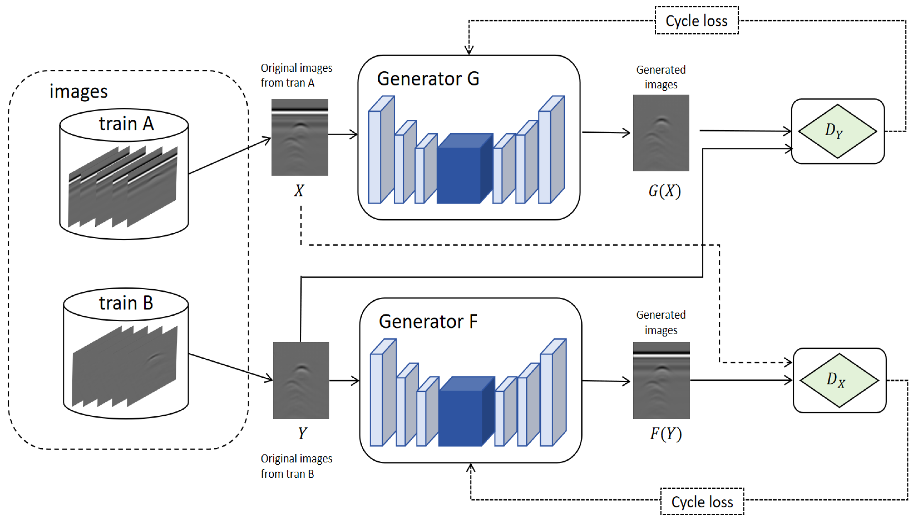
The overall network structure of the improved CycleGAN is shown in Figure 2.

First, the training dataset of the network is constructed. The dataset is divided into the clutter dataset A and the clutter-free dataset B. The data in the two datasets are used as inputs to generator $G$ and generator $F$, respectively. In this paper, the image domain storing clutter pipeline data is denoted as $X$, and the image domain storing pipeline data without clutter is denoted as $Y$. The process of clutter suppression is to use the generator $G$ to convert the GPR B-scan image with clutter into a GPR B-scan image without clutter. The process of clutter suppression is shown in Figure 3.

The network contains two generators and two discriminators. The two generators have the same structure and learn two mappings, $G:X\to Y$ and $F:Y\to X$, respectively. Among them, $X$ and $Y$ respectively represent two different GPR image domains. The $X$ domain contains GPR images with clutter, and the $Y$ domain contains GPR images with only target responses. At the same time, the network contains two adversarial discriminators, and the two discriminators $D_X$ and $D_Y$ also have the same structure. Among them, $D_X$ is used to distinguish whether the input image is a real image of the domain or an image generated by the generator $F$, and $D_Y$ is used to distinguish whether the input image is a real image of the domain or an image generated by the generator $G$. At the same time, the parameters of the two generators are updated through cycle loss. Cycle loss uses L₁ norm to regularize the model, and to avoid dependence on simulated data during model training, the network uses other graphs in the dataset to test the generators, further preventing over-fitting problems of generators $G$ and $F$.

Through training, the network can learn generator $G$ and generator $F$ at the same time, thereby generating images with similar feature distributions to image domain $Y$ and image domain $X$ respectively. However, in the process of clutter suppression, if the network has a large enough capacity, although the cluttered GPR data can be mapped into the clutter-free data target domain $Y$, these randomly generated clutter-free images have absolutely no relationship with the input.

To solve the above problems, CycleGAN also introduces forward cycle consistent loss and backward cycle consistent loss respectively. The forward cycle consistent loss requires that all images x in the $X$ domain can be transformed and recycled through image conversion and finally, restored to the original image, which is $x\to G\left(x\right)\to F\left(G\right(x\left)\right)\approx x$, the backward loop consistent loss is similar to the former, which is $y\to F\left(y\right)\to G\left(F\right(y\left)\right)\approx y$.

During training, the network optimizes the network by setting a loss function that calculates the difference between the output generated by the generator and the real image. The CycleGAN network sets three loss functions, namely cycle consistency loss, GAN loss, and identity loss. The cycle consistency loss and identity loss are both calculated using L₁ distance loss. Taking forward cycle consistency loss as an example, the expression of L₁ distance loss is as follows:

$$L_{L_1}\left(G\right)=‖y-G\left(x\right)‖$$

(6)

where $x$ represents the input GPR clutter data, $y$ represents the GPR clutter-free data, $G$ is the generator, and $G\left(x\right)$ represents the output of the network. The calculation of L₁ distance loss allows the network to continuously approach the true value in the sense of L₁ distance when generating data. Moreover, using the L₁ distance loss function to calculate the identity loss can also better retain some feature information of the original image.

However, during the training process of the network, to avoid the problem of losing some feature information of the generated image, the network introduces two discriminators at the same time and introduces an adversarial loss function $L_{GAN}$. The generator and the discriminator are jointly trained. In the adversarial loss function $L_{GAN}$, the generator’s goal is to minimize the loss $L_{GAN}$, and the discriminator’s goal is to maximize the loss $L_{GAN}$.This paper updates the generator parameters through the adversarial loss function $L_{GAN}$, thereby producing a clutter-free image that is indistinguishable from the real image. This paper extracts the feature information of the target response, discriminates the key feature information, and averages all the discrimination results to obtain the final output result.

3.2. Improve Generator and Discriminator

3.2.1. Generator Construction

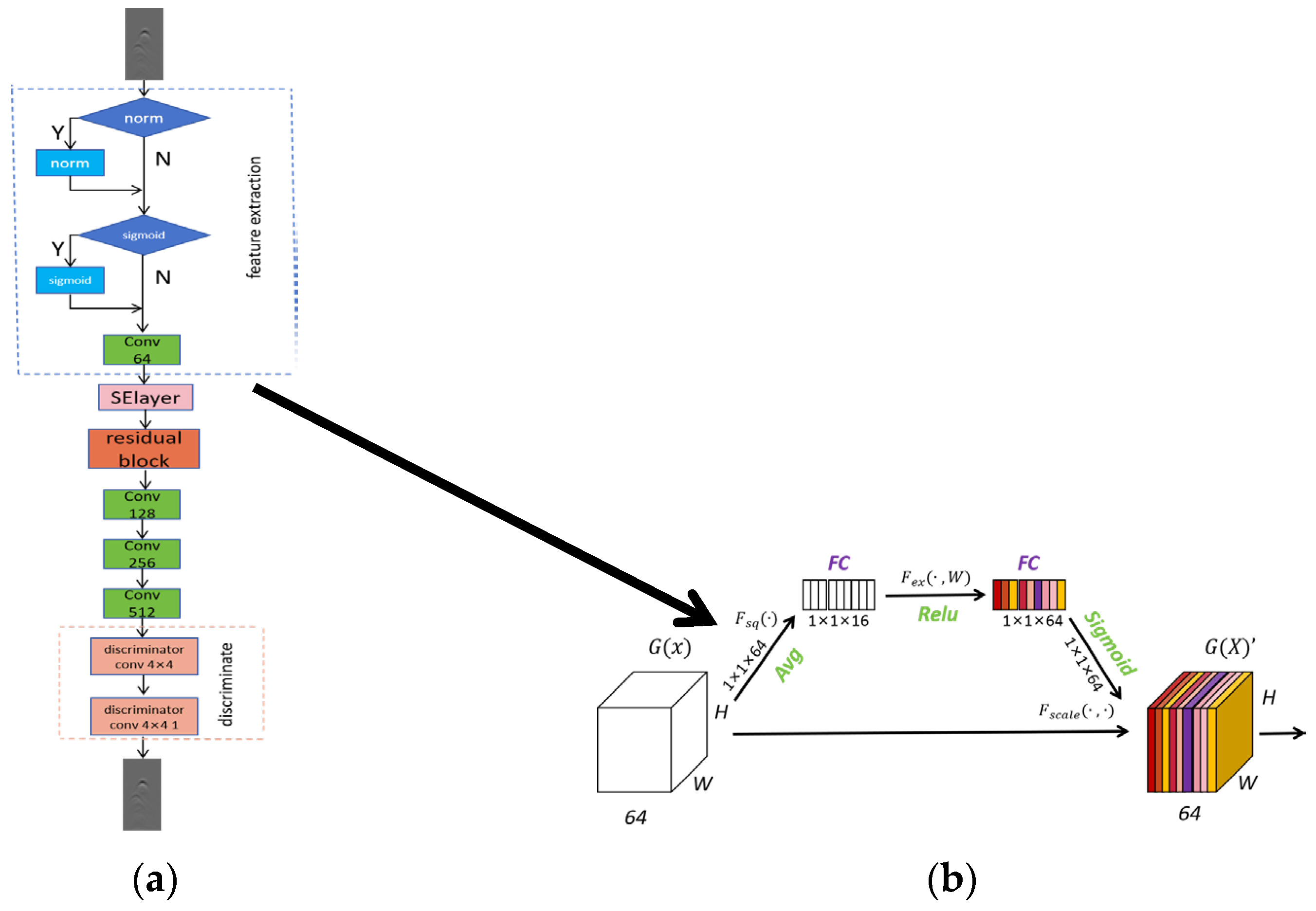
The generator $G$ and $F$ generator of CycleGAN have the same structure, and the structure of the generator is shown in Figure 4a.

The function of the generator $G$ is to convert the original clutter-containing data into clutter-free data after clutter suppression, and the generator $F$ is to add clutter to the clutter-free data and convert it into clutter-containing data. The construction of the generator in this paper consists of three parts, namely the feature extraction module, the feature reconstruction module, and the image up sampling module. The input GPR image is first resized into an image with 64 $\times$ 256 pixels. Then, the feature information of the GPR image is extracted through multiple convolutions and down-sampling until the end of the feature reconstruction layer, and then up-sampling restores the scale of the image. In the feature extraction module, it consists of a filling layer and two convolution layers. First, a filling layer is constructed to prevent the image from losing resolution after passing through the convolution layer. Then there is a convolution layer with a kernel of 7 $\times$ 7, which is used to increase the input channel to 16. Finally, there is a convolution layer with a kernel of 3 $\times$ 3 for extracting feature information. During convolution, batch normalization and activation functions are performed on the image to improve the representation ability of the network.

The extracted image feature information is input to the feature reconstruction module. The function of this module is to reconstruct the features and further process the features. The feature reconstruction module of the original CycleGAN has a simple structure, consisting of only one filling layer and one convolution layer, and cannot process complex clutter feature information on GPR data detected by GPR underground pipelines. Moreover, considering that during the underground pipeline detection process of GPR, there is overlap between the target response and clutter, which seriously affects the network’s learning of the global characteristics of the target response. Therefore, to solve the problem of partial feature information loss during the target response generation process, after feature extraction, a four-layer residual module is added to replace the feature reconstruction module of the original CycleGAN. The idea of residual network was first proposed by Zhang et al. in the literature [29]. The function of this module is to improve the generalization ability of the model, retain more useful information, and suppress useless information. Unlike the original CycleGAN network generator, the feature extraction effect is significantly improved through the skip connection part of the residual network.

The structure of the residual module is shown in Figure 4b. It consists of two filling layers and two convolutional layers. The two convolutional layers are kernel 3 $\times$ 3 convolutions. The convolution process also requires batch normalization and activation functions to improve the operating efficiency of the network. In the input part, a skip connection is implemented to incorporate the image features extracted using the feature extraction module with the features obtained through residual convolution. This enables the generation of a new image feature that incorporates both sets of extracted features. Due to the reference of skip connections, the global features of the image can be better preserved.

Lastly, the image upsampling module is employed to restore the original image pixels and revert the number of image channels to match the input’s channel count. The upsampling part consists of a transposed convolution module, which is a transposed convolution with a kernel of 3 $\times$ 3. In the process of upsampling deconvolution, batch normalization and activation functions are still performed to improve the feature expression ability of the network. Then, the image information is further retained through a filling layer and a convolution layer with a kernel of 7 $\times$ 7, and finally the generated result of the generator is output.

3.2.2. Discriminator Construction

The discriminator $D_X$ and discriminator $D_Y$ of CycleGAN also have the same structure. The structure of the discriminator is shown in Figure 5a.

The discriminator $D_X$ is used to distinguish whether the input image is a real image in the $X$ domain or an image generated by the generator $F$; $D_Y$ is used to distinguish whether the input image is a real image in the $Y$ domain or an image generated by the generator $G$. The discriminator in this paper consists of four parts, namely the feature extraction module, the attention mechanism module, the residual module, and the discriminant module. The discriminator is used to classify the input data and determine whether they are real data or generated data.

The original CycleGAN discriminator has a simple structure and only consists of a feature extraction part and a discrimination module. The discriminator first extracts features from the input image. During the feature extraction process, the feature discrimination results of the local area will affect the discrimination results of the entire image. Sometimes even if the local features of the target response are poorly generated or even missing, the discriminator will still judge the overall image as true. Therefore, only using CycleGAN’s original discriminator $D_X$ to discriminate the generated clutter-free image $G\left(x\right)$ will have the problem of poor local target response generation. To enhance the generation effect of target response, this paper introduces the channel attention mechanism SE module and residual module based on the original CycleGAN discriminator.

Among them, the channel attention mechanism SE module was first proposed by Hu in the literature [30]. This module can establish the interdependence between convolutional feature channels to improve the feature extraction capability of the network. The channel attention mechanism is introduced to enable the network to perform feature recalibration, through which global information can be effectively preserved, thereby selectively increasing the degree of attention to target response characteristic information and suppressing the degree of attention to useless characteristic information caused by useless clutter interference. At the same time, it helps the model better extract the hyperbolic features of the target response and avoids the discriminator being affected by irrelevant feature areas. The structure of the SE module of the attention mechanism is shown in Figure 5b. It mainly consists of a global average pooling layer and two fully connected layers, as well as the corresponding activation functions ReLu and Sigmoid of the fully connected layer. The discriminator retains the characteristic information of the target response through the attention mechanism, then further extracts features through the residual module, and finally obtains the final discrimination result through the discriminant module.

4. Data Preparation and Processing

The CycleGAN network is built on the basis of cycle consistency, allowing it to be trained separately using the data in the clutter dataset A and the clutter-free dataset B. Both datasets serve different purposes. Dataset A contains two parts, including the public dataset and the simulation dataset. The clutter data in dataset A can be input to the generator $G$ as data in the image domain $X$, thereby generating the clutter-free data $G\left(x\right)$. At the same time, it can also be used as a criterion to be input into the discriminator $D_X$ to determine the generation effect of the cluttered data $F\left(y\right)$ generated from the clutter-free data $y$ in the dataset B. Dataset B is a clutter-free dataset based on simulation, and its function is similar to dataset A. To verify the experiment, a measured dataset was also prepared. The prepared GPR dataset is shown in Figure 6.

4.1. CLT-GPR Public Dataset

The clutter-GPR (CLT-GPR) public dataset is a pipeline detection GPR dataset containing various real clutters proposed in the literature [26]. In the process of existing clutter removal tasks, the dataset only contains synthetic data [13,24], and this purely data-driven approach cannot learn the complex clutter distribution in real radar detection images. Due to the above problems, the CLT-GPR dataset is proposed to enrich the clutter types to solve the problem. This dataset uses the open-source software gprMax 3.0 [31] to generate the GPR dataset, and the simulation scene is shown in Figure 7a. The size of the simulation domain is 100 $\times$ 15 $\times$ 40 ${\mathrm{c}\mathrm{m}}^3$, and the grid size of the simulation domain is set to 0.002 m. A 1.5 GHz GSSI antenna is used as the transceiver [32], located 0.05 m above the soil surface. The antenna moves in a step of 0.01 m on the X-axis, and 80 A-Scan images are collected along the scanning trajectory to generate a B-scan image. To generate a synthetic dataset of multiple underground scenes, four types of surfaces, six types of soil, two types of objects, and three types of underground objects with different depths and radii were modeled during the simulation. By increasing the clutter richness of underground scenes in the dataset, the generalization ability of network training is improved. This dataset contains 14,000 simulated clutter datasets and clutter-free datasets. The data with clutter are stored in the training dataset A of the network, and the data without clutter are stored in the training dataset B. The data with clutter are shown in Figure 7b and the data without clutter are shown in Figure 7c.

4.2. GPR Public Dataset

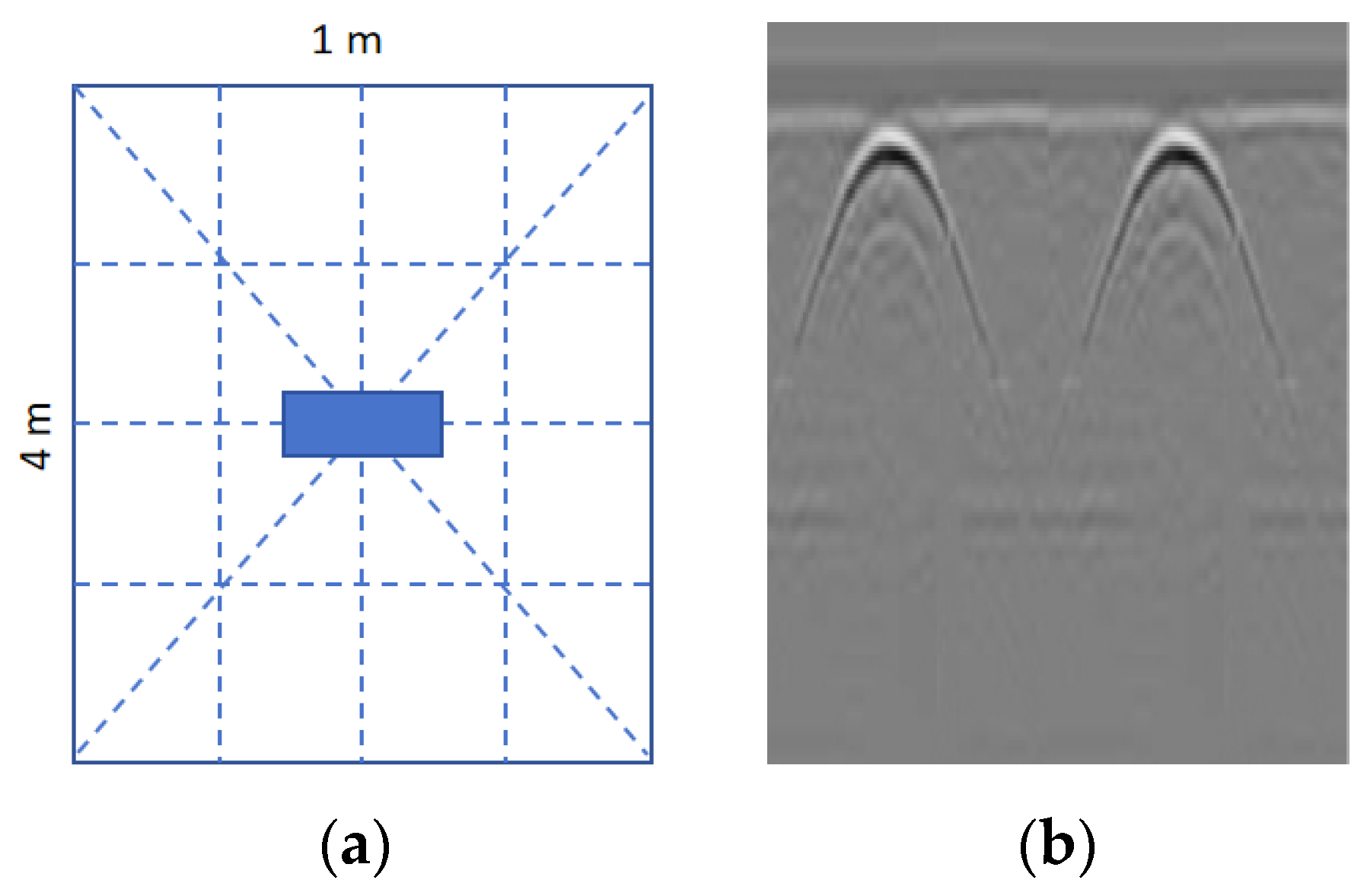
Create a parameter model during the simulation process to generate a simulation dataset for GPR pipeline inspection. The dimensions of the model are 1.0 m $\times$ 4.0 m (length $\times$ width). The schematic diagram of the scene model of simulation detection is shown in Figure 8a. Add nonuniform media to the model to simulate background clutter. On the near surface of the ground is a row of pipelines, and the location of the pipelines is at the grid line in Figure 8a. This paper used gprMax software for simulation. GprMax is an open-source software for electromagnetic wave propagation simulation. It solves the application problem of Maxwell’s equations in three dimensions based on the FDTD method. This software is mainly used for simulation and modeling of GPR, so the paper used gprMax software to create synthetic GPR pipeline data. The center frequency of the waveform is 1600 MHz, the time window is set to 15 ns, and the grid size of the simulation domain is set to 0.005 m. The simulation experiment uses a Hertz pulse dipole source to simulate the ground-penetrating radar emission source. The emission source is placed on the Z axis, the position is set to 0.1 m, the emission frequency is set to 1.5 GHz, and the initial phase is 0 radians. Set the coordinate position of the radar receiver to (0.2, 0.7, 0). The transmitter and receiver will move in steps of 0.01 m in the X-axis direction while remaining unchanged in the Y and Z-axis. Through FDTD simulation, a total of 600 GPR clutter-containing images were obtained. Pipeline parameters were added to generate clutter-containing images of a single pipeline and multiple pipelines. The generated GPR data are shown in Figure 8b.

4.3. Measured Dataset

During the simulation process, an underground soil hidden pipeline detection model with a size of 3.0 m $\times$ 5.0 m (length $\times$ width) was created, as shown in Figure 9a. By setting the number of pipelines, pipeline material, pipeline diameter, pipeline burial depth, etc., a total of 63 working conditions are set. The number of pipelines is set to single pipeline or multiple pipelines; the pipeline material is polyethylene or cast iron, the pipe diameter is 100/150/200/250 mm, and the pipeline burial depth is set to 10/15/20 cm. The paper used GPR to detect the actual scene. The number of sampling points is 2048, the sampling frequency is 4 GHz, and the detection time window is set to 50 ns.

As shown in Figure 9b, the paper obtained the original GPR B-scan data from the measured model. Because the training network needs to adjust the data size to 64 $\times$ 256, the size of the measured data is large, and the direct compression process will cause the target response and clutter features to be lost. To prevent missing data features, the original real images are preprocessed. The data are cut using a sliding cut method. Because the resolution of the measured data is relatively high, a sliding frame method is used to crop the images in the measured dataset to a suitable size. This method enriches the amount of data and enables detection. The effect of the picture is better than the effect of just detecting one picture. After preprocessing the measured data, the paper obtained 50 pieces of measured original GPR data.

5. Experiment Analysis

In this chapter, this paper used the CLT-GPR dataset in the literature [26] as the training data of the network and tested the simulation data and measured data to verify the clutter suppression effect of the network. The ratio of training set to test set was adjusted to 9:1. The following will be divided into three parts, as follows: first, the specific details of network training are introduced, and secondly, the evaluation indicators used in the experimental verification process are explained. Finally, the clutter suppression effect of the network is analyzed by comparing it with other methods.

5.1. Network Training

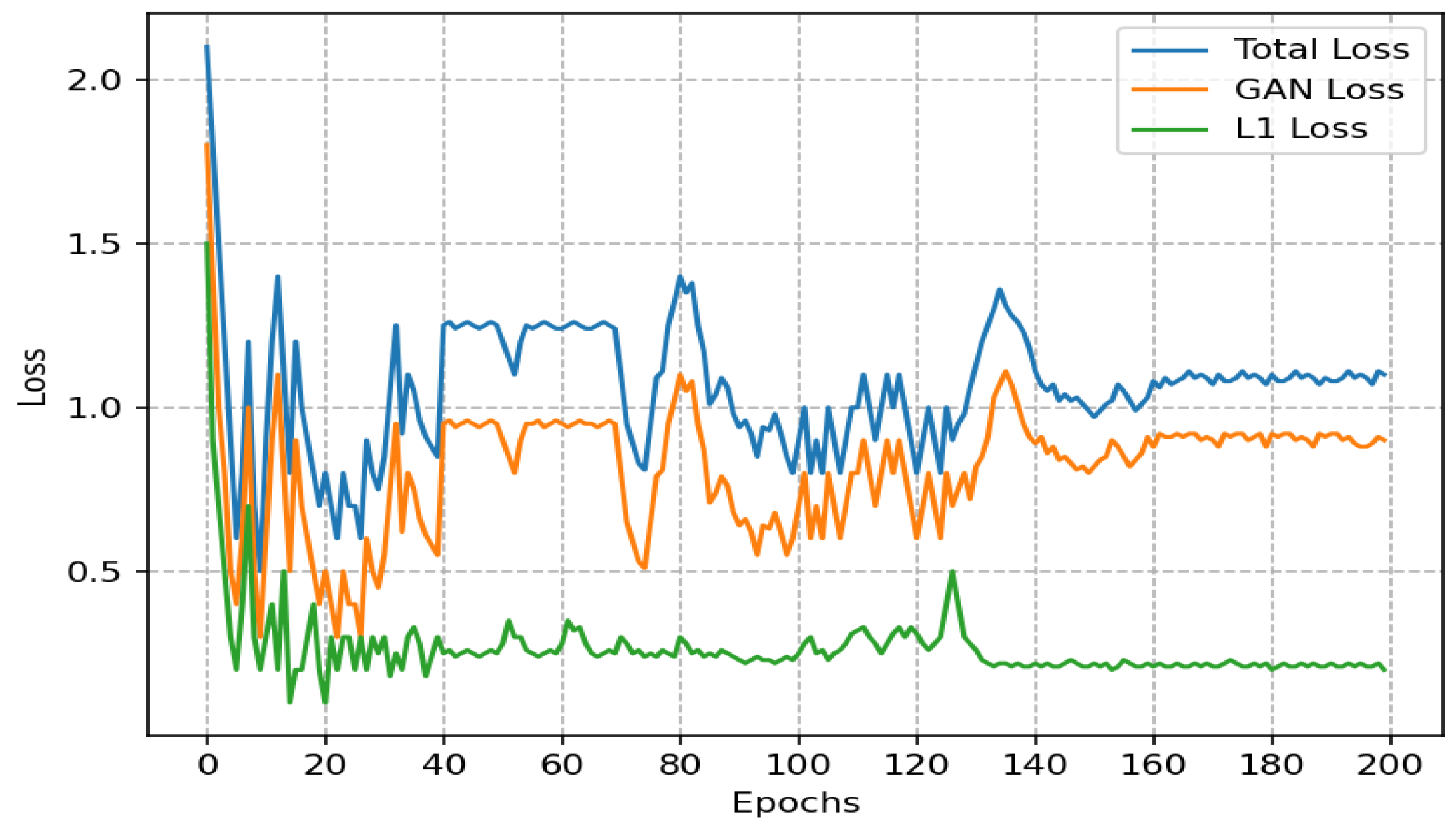
The data used for network training are the CLT-GPR dataset. The data are divided into dataset A and dataset B. Dataset A stores clutter data, and dataset B stores clutter-free data. In addition, datasets A and B are divided into training sets and test sets, respectively, according to the ratio of 9:1. The entire training process is carried out in Pytorch, using an i7-12700H CPU to build the network, with an RTX 3060 GPU. This study sets network training into two modes, so that the network can be trained through the original CycleGAN network structure or the improved CycleGAN network structure. The network uses ADAM optimizer for network parameter optimization [33], setting the learning rate and decay rate to 0.0002 and 0.5, respectively, setting the batch size to eight, and setting the data size to 64 $\times$ 256, then normalizing it to the [0, 1] range. The data in the training set are input into the network and trained for 200 epochs. The overall training time is about 6 h. To facilitate subsequent experiments, the initial training times are set when building the model, so that iterations can continue based on the trained weights and avoid the time consumed by retraining. Finally, the network effect is tested using the data of the test set. The loss curve during training is shown in Figure 10.

5.2. Evaluation Index

5.2.1. Evaluation Indicators for Simulation Experiments

The simulated underground pipeline B-scan data have corresponding clutter-free images for comparison. Therefore, to evaluate the clutter suppression effect of simulation data, this paper will use the two quantitative indicators, including mean squared error (MSE) and peak signal-to-noise ratio (PSNR), as defined in [34], to evaluate the clutter suppression effect and performance of different methods. Both MSE and PSNR are used to calculate the degree of difference between the results after clutter suppression and the expected results. The two indicators are defined as follows:

$$MSE=\frac{1}{H\times W}\sum _{i,j}{(y_{i,j}-{\widehat{y}}_{i,j})}^2$$

(7)

$$PSNR(dB)=20·{\mathit{log}}_{10}(\frac{{MAX}^2}{MSE})$$

(8)

In Equation (6), $y_{i,j}$ and ${\widehat{y}}_{i,j}$ are, respectively, the clutter-free image after network processing and the clutter-free data corresponding to the image size $H\times W$ in the simulation dataset. In Equation (7), $MAX$ represents the maximum possible value of 255 for the image pixel value.

Throughout the experiment, lower MSE values and higher PSNR values after clutter suppression indicate that the resulting clutter-free image closely resembles the real simulation data. This signifies that the network’s clutter suppression effect is superior.

5.2.2. Evaluation Indicators for Actual Experiments

Because true images without clutter cannot be obtained during the actual radar detection process, the evaluation indicators of simulated data cannot evaluate the actual measured data. Therefore, this paper used the improvement factor Im [35] to quantitatively evaluate the performance of different clutter suppression methods. The improvement factor is defined as the ratio between the signal-to-clutter ratio (SCR) of the clutter-suppressed radar image and the SCR of the unprocessed original radar image, where Im is defined as follows in Equation (8):

$$Im(dB)=20\ast {\mathit{log}}_{10}\frac{{SCR}_{processed}}{{SCR}_{raw}}$$

(9)

The SCR is defined as the ratio of the energy of the target response to the clutter energy. The energy depends on the sum of the squares of each pixel in the image. The definition of SCR is as follows in Equation (9):

$$SCR=10\ast {\mathit{log}}_{10}\frac{E_{signal}}{E_{clutter}}$$

(10)

The definitions of $E_{signal}$ and $E_{clutter}$ in Equation (9) are as shown in Equations (10) and (11), respectively, as follows:

$$E_{signal}={\sum }_{i,j}{z_{i,j}}^2$$

(11)

$$E_{clutter}=\sum _{i,j}{{(x}_{i,j}-y_{i,j})}^2$$

(12)

When calculating $E_{signal}$, $z_{i,j}$ is represented as the pixel point of the image. When calculating ${SCR}_{processed}$, $z_{i,j}$ represents the pixels of the radar image after clutter suppression. When calculating $E_{clutter}$, ${SCR}_{processed}$ and ${SCR}_{raw}$ are calculated in the same way. The pixel points of the original unprocessed radar image are compared with the pixel points of the radar image after clutter suppression, and the squares of the differences are summed.

5.3. Analysis of Results

5.3.1. Simulation Data Experimental Verification

The experimental results based on the simulation dataset are shown in Figure 11. The first column is the unprocessed original GPR image. To compare with the traditional clutter suppression method, this paper reproduces two subspace-based clutter suppression methods. The second column is the SVD singular value decomposition method. The third column is the RPCA low-rank sparse decomposition method. This paper also compares the algorithm with clutter suppression methods based on deep learning. The fourth and fifth columns are clutter suppression methods based on deep learning, which are U-Net and the original CycleGAN, respectively. The last column is the improved CycleGAN clutter suppression results.

In Figure 11, it can be seen that although SVD and RPCA can suppress most of the clutter, a small amount of residual clutter will merge with the target response, seriously affecting the generation of the target response and even weakening the generation of some target responses, which is more obvious under S2. Methods based on deep learning are effective in removing background clutter, but they will still distort or weaken the target response. In contrast, the improved CylcleGAN network in this paper successfully eliminates most of the clutter and better retaining the target response. Our improved network has very significant effects in S1 and S2. The evaluation indicators of the simulation data experiment are shown in

Table 1. Quantitative comparison of the performance of different clutter suppression methods under S1. Among them, a smaller value of MSE is better, while a larger value of PSNR is desired. The figures will be represented using arrows.

Methods	SVD	RPCA	U-Net	CycleGAN	Our
MSE (↓)	0.03	0.02	0.008	0.002	0.001
PSNR (↑)	42.43	45.95	53.36	54.80	66.95

and

Table 2. Quantitative comparison of the performance of different clutter suppression methods under S2. Among them, a smaller value of MSE is better, while a larger value of PSNR is desired. The figures will be represented using arrows.

Methods	SVD	RPCA	U-Net	CycleGAN	Our
MSE (↓)	0.026	0.015	0.007	0.006	0.0007
PSNR (↑)	43.67	48.65	54.66	55.26	73.97

. It can be seen in the table that the MSE and PSNR of the network in both cases are better than the previous traditional methods and deep learning-based methods.

5.3.2. Measured Data Experimental Verification

This study utilizes GPR B-scan images obtained from physical model experiments to validate the effectiveness of the improved network for clutter suppression proposed in this paper. At the same time, the practicality of the proposed method for GPR underground pipeline data processing is verified in the actual environment.

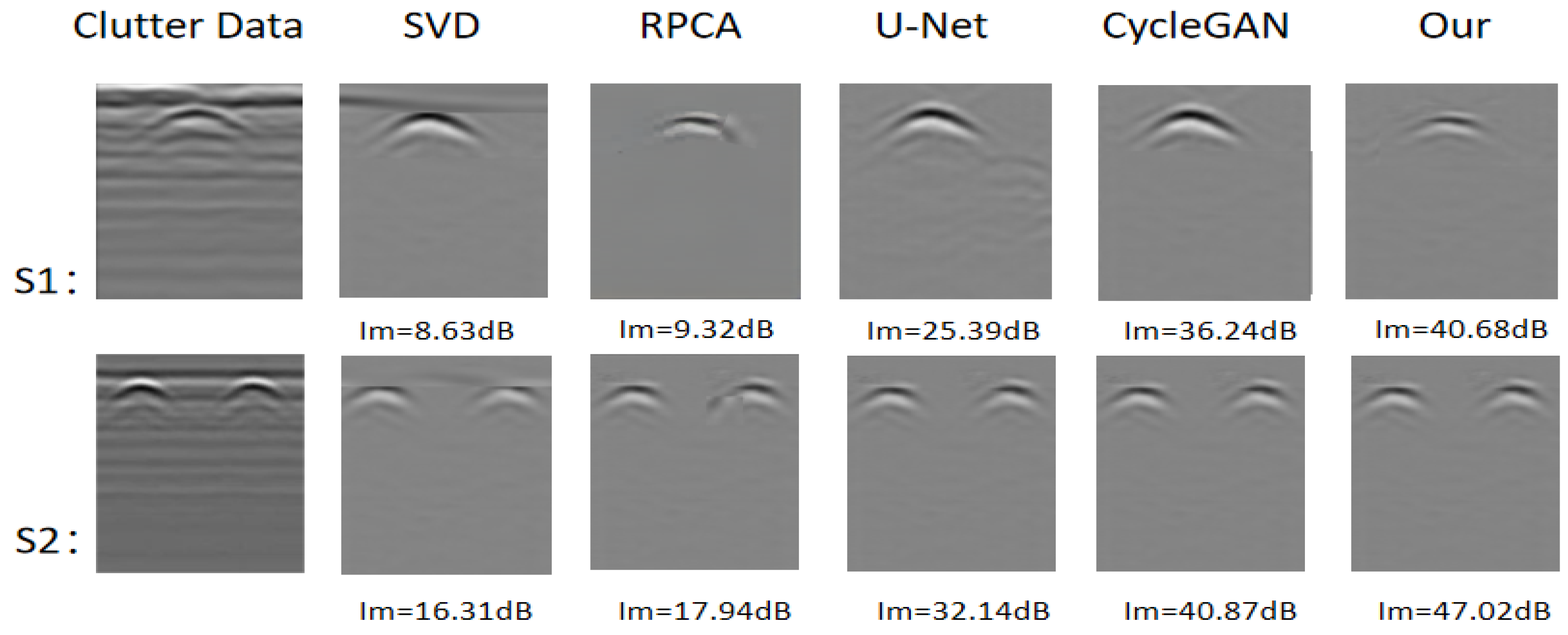
As shown in the first column of Figure 12, the second and third columns are the results with traditional clutter suppression method, the second column is the SVD singular value decomposition method, and the third column is the RPCA low-rank sparse decomposition method. The fourth and fifth columns are the results of the clutter suppression method based on deep learning, of which the fourth column is U-Net, and the fifth column is the original CycleGAN. The last column is the network clutter suppression effect improved by this paper.

As can be seen in Figure 12, SVD and RPCA cannot remove some background clutter. The deep learning methods U-Net and CycleGAN have shown good capabilities in eliminating GPR clutter, but they still have the problem of weakening or distorting some target responses. The improved CycleGAN network in this paper has significant improvements compared with traditional methods and deep learning methods. When removing background clutter, it can retain most of the characteristic information of the target response well. The improvement factor Im has increased to 40.68 dB in the measured data of a single pipeline compared with the previous instance and has also increased to 47.02 dB in the measured data of multiple pipelines.

To improve the generalization ability of the model, this paper validated the clutter suppression effects of different measured data, and the comparison results are shown in Figure 13.

From Figure 13, it can be observed that the network proposed in this paper can effectively remove clutter in actual scenes and exhibits good clutter suppression effects in different scenarios. However, through analysis, it was found that the overall performance of actual measurement experiments has decreased compared to simulation experiments. The main reasons are as follows:

This paper uses GPR data simulated based on gprMAX simulation software for training. The simulated clutter data are put into the training dataset A, and the simulated clutter-free data are put into the training dataset B. Finally, the simulation data and measured data are verified. However, due to the influence of the training set, because the measured data make it difficult to provide clutter-free data, and the underground detection in the actual environment is more complicated, the GPR clutter-free data simulated in this paper during the training process will be different from the real situation.

6. Conclusions

This paper proposes an improved clutter suppression method based on the CycleGAN network. The objective of constructing the CycleGAN network is to effectively eliminate clutter while preserving the pipeline response in B-scan images during GPR pipeline detection. In the network, this paper improves the conventional CycleGAN network by incorporating residual learning and channel attention mechanisms. The two modules further enhance CycleGAN’s ability to identify clutter. Furthermore, experimental analysis is performed to compare the improved CycleGAN network with other networks. Extensive experimental results demonstrate that the improved CycleGAN can automatically and effectively remove clutter from measured GPR radar images. Notably, it does not require paired clutter and non-clutter data for training, showcasing its exceptional generalization ability for radar image processing in real-world scenarios. In the real environment, this method has a better clutter suppression effect on GPR pipeline data than other methods and does not require the manual adjustment of hyperparameters. It can produce clutter-free images with good target response recovery. It is beneficial for subsequent image analysis, such as underground target imaging, positioning, and identification. However, only simulation data were used during the training process, so it has limitations when applied to complex scenarios. The proposed network in this paper does not rely on paired data for training, offering the potential for further performance improvement by incorporating real data into the training process. Nevertheless, the current availability of real data remains insufficient. In our future work, we plan to collect a larger volume of real data for training, aiming to enhance the network’s generalization ability.

References

1. Daniels, D.J. Ground Penetrating Radar, 2nd ed.; IEEE Press: London, UK, 2004; Available online: https://digital-library.theiet.org/content/books/ra/pbra015e (accessed on 20 January 2024).
2. Liu, Z.; Gu, X.; Wu, W.; Zou, X.; Dong, Q.; Wang, L. GPR-based detection of internal cracks in asphalt pavement: A combination method of DeepAugment data and object detection. Measurement 2022, 197, 111281. [Google Scholar] [CrossRef]
3. Jol, H.M. Ground Penetrating Radar Theory and Applications; Elsevier: Amsterdam, The Netherlands, 2008; Available online: https://www.sciencedirect.com/book/9780444533487/ground-penetrating-radar-theory-and-applications (accessed on 20 January 2024).
4. Ito, T.; Katayama, R.; Manabe, T.; Nishibori, T.; Haruyama, J.; Matsumoto, T.; Miyamoto, H. Preliminary Study of a Ground Penetrating Radar for Subsurface Sounding of Solid Bodies in the Solar System. In Proceedings of the 2013 International Symposium on Antennas & Propagation, Nanjing, China, 23–25 October 2013; Available online: https://ieeexplore.ieee.org/document/6717411 (accessed on 20 January 2024).
5. Zhang, X.; Bolton, J.; Gader, P. A New Learning Method for Continuous Hidden Markov Models for Subsurface Landmine Detection in Ground Penetrating Radar. IEEE J. Sel. Top. Appl. Earth Obs. Remote Sens. 2014, 7, 813–819. [Google Scholar] [CrossRef]
6. Zhang, C.; Yu, J.; Wu, J.; Li, Z.; Zhu, L. Application of Ground-Penetrating Radar Broadband Antenna in Underground Detection. E3S Web Conf. 2020, 198, 04005. [Google Scholar] [CrossRef]
7. Ozkaya, U.; Melgani, F.; Belete Bejiga, M.; Seyfi, L.; Donelli, M. GPR B scan image analysis with deep learning methods. Measurement 2020, 165, 107770. [Google Scholar] [CrossRef]
8. Nan, F.; Zhou, S.; Wang, Y.; Li, F.; Yang, W. Reconstruction of GPR Signals by Spectral Analysis of the SVD Components of the Data Matrix. IEEE Geosci. Remote Sens. Lett. 2010, 7, 200–204. [Google Scholar] [CrossRef]
9. Karlsen, B.; Larsen, J.; Sorensen, H.; Jakobsen, K.B. Comparison of PCA and ICA based clutter reduction in GPR systems for anti-personal landmine detection. In Proceedings of the 11th IEEE Signal Processing Workshop on Statistical Signal Processing (Cat. No.01TH8563), Singapore, 8 August 2001; Available online: https://ieeexplore.ieee.org/document/955243 (accessed on 20 January 2024).
10. Song, X.; Xiang, D.; Kai, Z.; Su, Y. Improving RPCA-Based Clutter Suppression in GPR Detection of Antipersonnel Mines. IEEE Geosci. Remote Sens. Lett. 2017, 14, 1338–1342. [Google Scholar] [CrossRef]
11. Zhou, T.; Tao, D. Godec: Randomized Low-Rank & Sparse Matrix Decomposition in Noisy Case. In Proceedings of the 28th International Conference on Machine Learning, ICML, Bellevue, WA, USA, 28 June–2 July 2011; pp. 33–40. [Google Scholar]
12. Sahin, S.; Hocaoglu, A.K. Non-Negative Matrix Factorization Method for Ground Penetrating Radar Images. In Proceedings of the 2019 27th Signal Processing and Communications Applications Conference (SIU), Sivas, Turkey, 24–26 April 2019; pp. 1–4. [Google Scholar]
13. Zhou, H.; Wang, Y.; Liu, Q.; Wang, Y. RNMF-Guided Deep Network for Signal Separation of GPR Without Labeled Data. IEEE Geosci. Remote Sens. Lett. 2022, 19, 1–5. [Google Scholar] [CrossRef]
14. Krizhevsky, A.; Sutskever, I.; Hinton, G.E. ImageNet classification with deep convolutional neural networks. Adv. Neural Inf. Process. Syst. 2012, 25, 1097–1105. [Google Scholar] [CrossRef]
15. LeCun, Y.; Bengio, Y.; Hinton, G. Deep learning. Nature 2015, 521, 436–444. [Google Scholar] [CrossRef]
16. Tong, Z.; Gao, J.; Yuan, D. Advances of deep learning applications in ground-penetrating radar: A survey. Constr. Build. Mater. 2020, 258, 120371. [Google Scholar] [CrossRef]
17. Pham, M.T.; Lefévre, S. Buried object detection from B-scan ground penetrating radar data using Faster-RCNN. In Proceedings of the IEEE International Symposium on Geoscience and Remote Sensing IGARSS, Valencia, Spain, 22–27 July 2018; pp. 6804–6807. [Google Scholar]
18. Xu, X.; Lei, Y.; Yang, F. Railway subgrade defect automatic recognition method based on improved Faster R-CNN. Sci. Program. 2018, 2018, 4832972. [Google Scholar] [CrossRef]
19. Lei, W.; Hou, F.; Xi, J.; Tan, Q.; Xu, M.; Jiang, X.; Liu, G.; Gu, Q. Automatic hyperbola detection and fitting in GPR B-scan image. Autom. Constr. 2019, 106, 102839. [Google Scholar] [CrossRef]
20. Qin, H.; Zhang, D.; Tang, Y.; Wang, Y. Automatic recognition of tunnel lining elements from GPR images using deep convolutional networks with data augmentation. Autom. Constr. 2021, 130, 103830. [Google Scholar] [CrossRef]
21. Hou, F.; Qiao, B.; Dong, J.; Ma, Z. S-CycleGAN: A Novel Target Signature Segmentation Method for GPR Image Interpretation. IEEE Geosci. Remote Sens. Lett. 2024, 21, 7502005. [Google Scholar] [CrossRef]
22. Liu, Z.; Gu, X.; Chen, J.; Wang, D.; Chen, Y.; Wang, L. Automatic recognition of pavement cracks from combined GPR B-scan and C-scan images using multiscale feature fusion deep neural networks. Autom. Constr. 2023, 146, 104698. [Google Scholar] [CrossRef]
23. Ni, Z.-K.; Ye, S.; Shi, C.; Li, C.; Fang, G. Clutter suppression in GPR B-scan images using robust autoencoder. IEEE Geosci. Remote Sens. Lett. 2022, 19, 1–5. [Google Scholar] [CrossRef]
24. Temlioglu, E.; Erer, I. A novel convolutional autoencoder-based clutter removal method for buried threat detection in ground-penetrating radar. IEEE Trans. Geosci. Remote Sens. 2022, 60, 1–13. [Google Scholar] [CrossRef]
25. Wang, J.; Chen, K.; Liu, H.; Zhang, J.; Kang, W.; Li, S.; Jiang, P.; Sui, Q.; Wang, Z. Deep learning-based rebar clutters removal and defect echoes enhancement in GPR images. IEEE Access 2021, 9, 87207–87218. [Google Scholar] [CrossRef]
26. Sun, H.-H.; Cheng, W.; Fan, Z. Learning to Remove Clutter in Real-World GPR Images Using Hybrid Data. IEEE Trans. Geosci. Remote Sens. 2022, 60, 5113714. [Google Scholar] [CrossRef]
27. Zhu, J.-Y.; Park, T.; Isola, P.; Efros, A.A. Unpaired Image-to-Image Translation Using Cycle-Consistent Adversarial Networks. In Proceedings of the 2017 IEEE International Conference on Computer Vision (ICCV), Venice, Italy, 22–29 October 2017; pp. 2242–2251. [Google Scholar] [CrossRef]
28. Goodfellow, I.; Pouget-Abadie, J.; Mirza, M.; Xu, B.; Warde-Farley, D.; Ozair, S.; Courville, A.; Bengio, Y. Generative adversarial nets. In Advances in Neural Information Processing Systems; Curran Associates, Inc.: New York, NY, USA, 2014. [Google Scholar]
29. He, K.; Zhang, X.; Ren, S.; Sun, J. Deep Residual Learning for Image Recognition. In Proceedings of the 2016 IEEE Conference on Computer Vision and Pattern Recognition (CVPR), Las Vegas, NV, USA, 27–30 June 2016; pp. 770–778. [Google Scholar] [CrossRef]
30. Hu, J.; Shen, L.; Sun, G. Squeeze-and-Excitation Networks. In Proceedings of the 2018 IEEE/CVF Conference on Computer Vision and Pattern Recognition, Salt Lake City, UT, USA, 18–23 June 2018; pp. 7132–7141. [Google Scholar] [CrossRef]
31. Warren, C.; Giannopoulos, A.; Giannakis, I. gprMax: Open source software to simulate electromagnetic wave propagation for Ground Penetrating Radar. Comput. Phys. Commun. 2016, 209, 163–170. [Google Scholar] [CrossRef]
32. Giannakis, I.; Giannopoulos, A.; Warren, C. Realistic FDTD GPR antenna models optimised using a novel linear/nonlinear full waveform inversion. IEEE Trans. Geosci. Remote Sens. 2019, 57, 1768–1778. [Google Scholar] [CrossRef]
33. Kingma, D.P.; Ba, J. Adam: A Method for Stochastic Optimization. arXiv 2017, arXiv:1412.6980. [Google Scholar]
34. Vitebskiy, S.; Carin, L.; Ressler, M.A.; Le, F.H. Ultra-wideband, short-pulse ground-penetrating radar: Simulation and measurement. IEEE Trans. Geosci. Remote Sens. 1997, 35, 762–772. [Google Scholar] [CrossRef]
35. Skolnik, M.I. MTI radar. In Radar Handbook, 2nd ed.; McGraw-Hill: New York, NY, USA, 1990. [Google Scholar]
Figure 1. Principle structure diagram of CycleGAN. (a) The model consists of two mapping functions G: XY and F: YX, as well as related adversarial descriptors Dy and Dx. The cycle-consistent loss of CycleGAN is divided into forward cycle-consistent loss and backward cycle-consistent loss. (b) Forward loop consistency: XG(x) → F(G(x))~x and (c) Backward loop consistency loss: yF(y) → G(F(y))~y.
Remotesensing 16 01043 g001
Figure 2. Improved CycleGAN structure.
Remotesensing 16 01043 g002
Figure 3. Clutter suppression process.
Remotesensing 16 01043 g003
Figure 4. (a) Improved CycleGAN generator structure; (b) residual module network structure.
Remotesensing 16 01043 g004
Figure 5. (a) Improved CycleGAN discriminator structure; (b) channel attention mechanism network structure.
Remotesensing 16 01043 g005
Figure 6. (a) Single-pipeline GPR data; (b) multiple-pipeline GPR data. The first column of images is the cluttered images in the CLT-GPR public dataset; the second column of images is the simulated cluttered images; the third column is the measured dataset in the actual scene; and the fourth column is the CLT-GPR public data concentrated clutter-free images.
Remotesensing 16 01043 g006
Figure 7. (a) Schematic diagram of synthetic dataset simulation scenario; (b) simulation data with clutter; (c) simulation data without clutter.
Remotesensing 16 01043 g007
Figure 8. (a) Schematic diagram of GPR simulation detection scene; (b) GPR simulation data of dual pipeline detection.
Remotesensing 16 01043 g008
Figure 9. Actual measured underground pipeline detection model: (a) actual measurement scene; (b) collected original GPR B-scan data.
Remotesensing 16 01043 g009
Figure 10. Loss curve of network training process.
Remotesensing 16 01043 g010
Figure 11. Clutter suppression effect on simulation data: (S1) simulated single-pipeline data; (S2) simulated multi-pipeline data. The second and third columns describe the clutter suppression effects of traditional clutter suppression methods SVD and RPCA, respectively. The fourth and fifth columns describe the clutter suppression effects of the deep learning-based clutter suppression methods U-Net and CycleGAN, respectively. The sixth column is the clutter suppression effect of the improved network, and the last column is the simulated clutter-free data.
Remotesensing 16 01043 g011
Figure 12. Clutter suppression effect on actual measured data: (S1) actual measured single-pipeline data; (S2) actual measured multi-line data. The second and third columns describe the clutter suppression effects of traditional clutter suppression methods SVD and RPCA, respectively. The fourth and fifth columns describe the clutter suppression effects of the deep learning-based clutter suppression methods U-Net and CycleGAN, respectively, and the last column describes the clutter suppression effect of the improved network.
Remotesensing 16 01043 g012
Figure 13. The clutter suppression effect of different measured data: input: original measured data; output: effect image after clutter suppression. The first column is the publicly available NSGeophysics measurement dataset. The second column is the publicly available CMU-GPR measurement dataset. The third column is the publicly available measured dataset of the DR-GAN network. The fourth column is the measured dataset provided in this paper.
Remotesensing 16 01043 g013