Article

Farmland Segmentation in Landsat 8 Satellite Images Using Deep Learning and Conditional Generative Adversarial Networks

1
Centre for Computational Science and Mathematical Modelling, Coventry University, Coventry CV1 2TL, UK
2
Faculty of Science and Engineering, Swansea University, Swansea SA2 8PP, UK
*
Author to whom correspondence should be addressed.
Remote Sens. 2024, 16(5), 823; https://doi.org/10.3390/rs16050823
Submission received: 15 January 2024 / Revised: 13 February 2024 / Accepted: 23 February 2024 / Published: 27 February 2024
(This article belongs to the Section Remote Sensing Image Processing)

Abstract

:
Leveraging mid-resolution satellite images such as Landsat 8 for accurate farmland segmentation and land change monitoring is crucial for agricultural management, yet is hindered by the scarcity of labelled data for the training of supervised deep learning pipelines. The particular focus of this study is on addressing the scarcity of labelled images. This paper introduces several contributions, including a systematic satellite image data augmentation approach that aims to maintain data population consistency during model training, thus mitigating performance degradation. To alleviate the labour-intensive task of pixel-wise image labelling, we present a novel application of a modified conditional generative adversarial network (CGAN) to generate artificial satellite images and corresponding farm labels. Additionally, we scrutinize the role of spectral bands in satellite image segmentation and compare two prominent semantic segmentation models, U-Net and DeepLabV3+, with diverse backbone structures. Our empirical findings demonstrate that augmenting the dataset with up to 22.85% artificial samples significantly enhances the model performance. Notably, the U-Net model, employing standard convolution, outperforms the DeepLabV3+ models with atrous convolution, achieving a segmentation accuracy of 86.92% on the test data.

1. Introduction

Satellite images are an important source of data for agricultural and environmental studies, given their world-level view, especially for addressing the challenges induced by climate change, such as the considerable reduction in average crop yields. Nearly 800 million people in the world are in shortage of food supplies, and in a couple of decades, the food demand is expected to increase by 60% [1]. Remote sensing has helped in monitoring different land cover changes, including agricultural areas [2,3,4].
In connection to the agricultural domain, satellite images have proven to be effective in monitoring farmlands and agricultural fields. Traditional surveys of farmlands are expensive and labour-intensive. Remote sensing can help to extract pixel-level information from satellite images to develop sustainable agricultural methods and crop planning. The obtained information can empower various stakeholders to make better-informed decisions in order to tackle climate change challenges and increase yield productivity at the same time [5].
In order to conduct studies on the effects of climate change on agriculture, a long history of time series of satellite images, e.g., from previous decades, is required. One existing source of satellite imagery in this case is the Landsat collection. Landsat is one of the oldest and most robust satellite programs, launched by NASA in 1967. The program has maintained impressive continuity over the years [6]. However, Landsat images are in low spatial resolution, e.g., 30 m per pixel. Therefore, it remains a challenge to segment objects as the first step of the analysis pipelines for different purposes. Semantic segmentation of these images to identify farmlands is a crucial step to be able to predict the crop types and yield and monitor the health of crops.
This paper investigates three important factors in the segmentation of Landsat images, particularly in farm areas: the augmentation of data to compensate for the common problem of a lack of labelled pixels, the model architecture, and the type of spectral bands. We first pre-process and label the satellite images as one of two categories: farms and non-farms; then, we use the labelled patches of the data to perform semantic segmentation. In this study, we focus on supervised semantic segmentation strategies using deep learning models. The selection of the group of deep learning strategies is due to their superiority in terms of accuracy compared to other groups of feature extraction and classification methods as compared in previous studies [7,8,9,10]. One of the main challenges in training deep models is related to the limited availability of labelled images, which can cause model over-fitting and influence segmentation accuracy. Therefore, data augmentation is conducted. The common strategies for augmentation are based on applying noise or affine transformation to the images, which only increases the number of images while keeping the same array of mask labels between the augmented and original images. However, to the best of our knowledge, no previous studies have attempted to generate new masks besides images in the field of remote sensing for farmland segmentation using mid-resolution satellite imagery. We address this problem by training a CGAN [11] model. In terms of the models, two popular semantic segmentation pipelines based on U-Net [12] and DeeplabV3+ [13] are compared. We also evaluate the performance when leveraging transfer learning approaches using pre-trained networks. Furthermore, the influence of the spectral bands on the segmentation results is studied. The main contributions of this paper are summarized as follows:
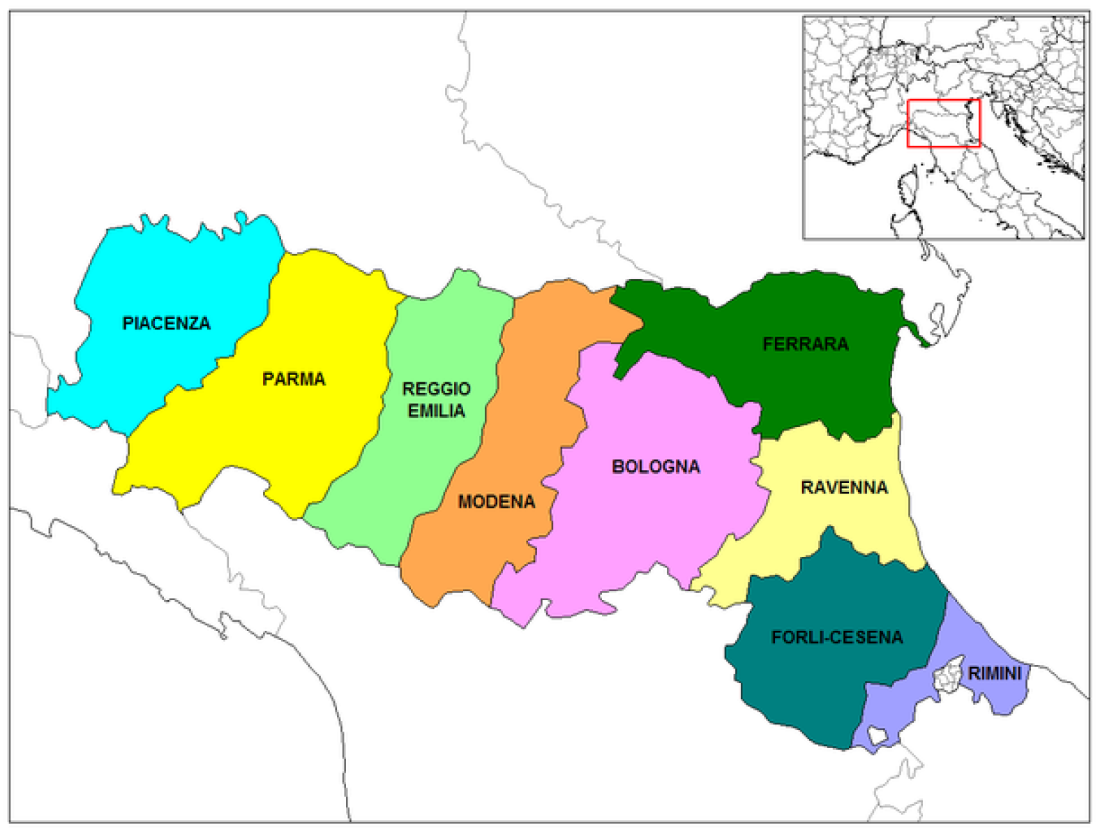
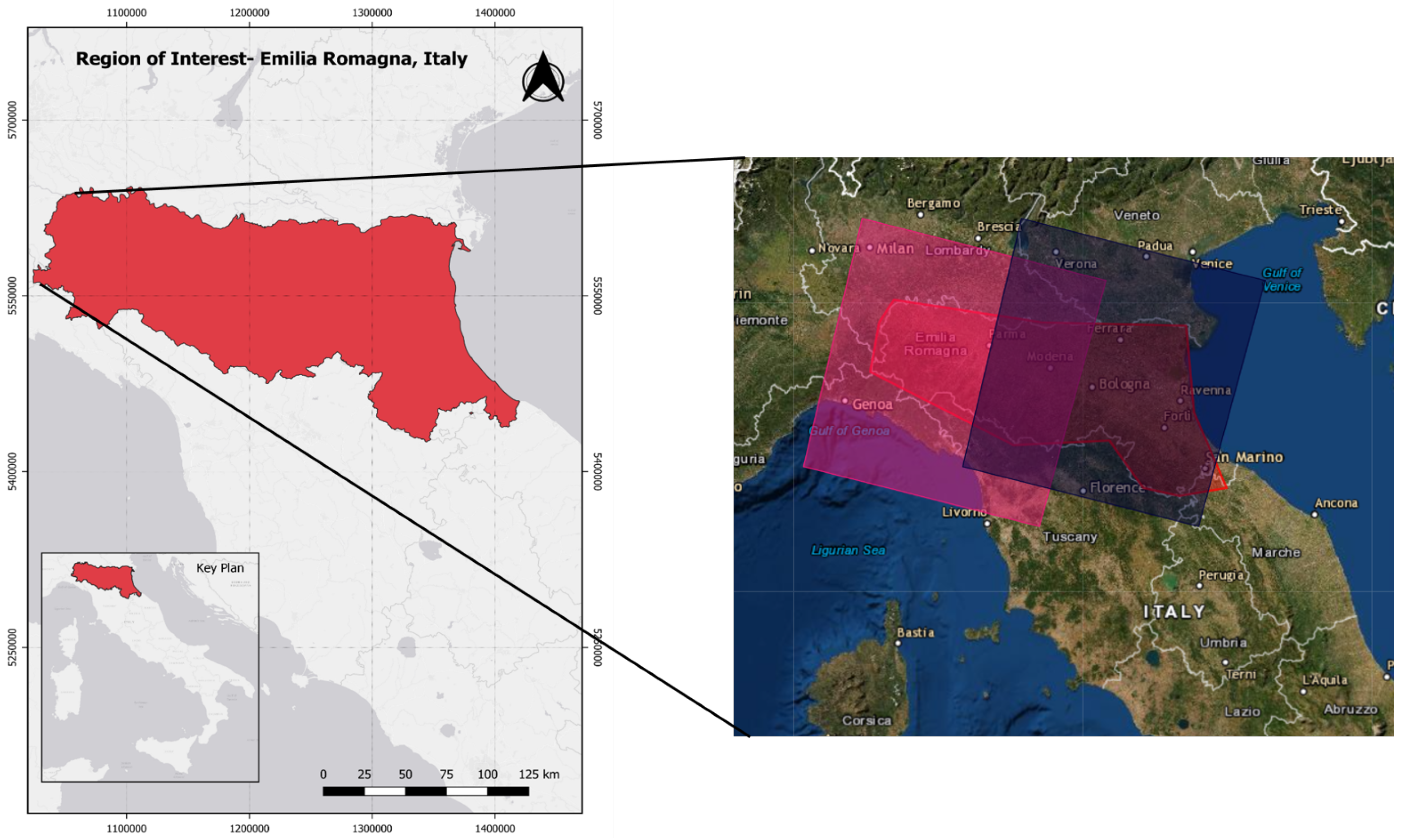
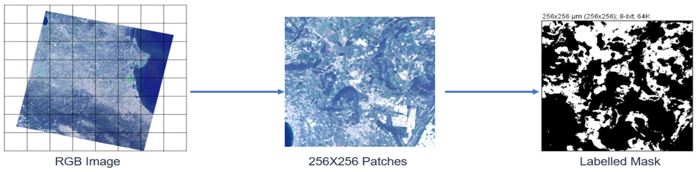
  • We develop a new labelled dataset of 30 m resolution Landsat 8 images with labelled farm and non-farm areas from the region of Emilia-Romagna in Italy.
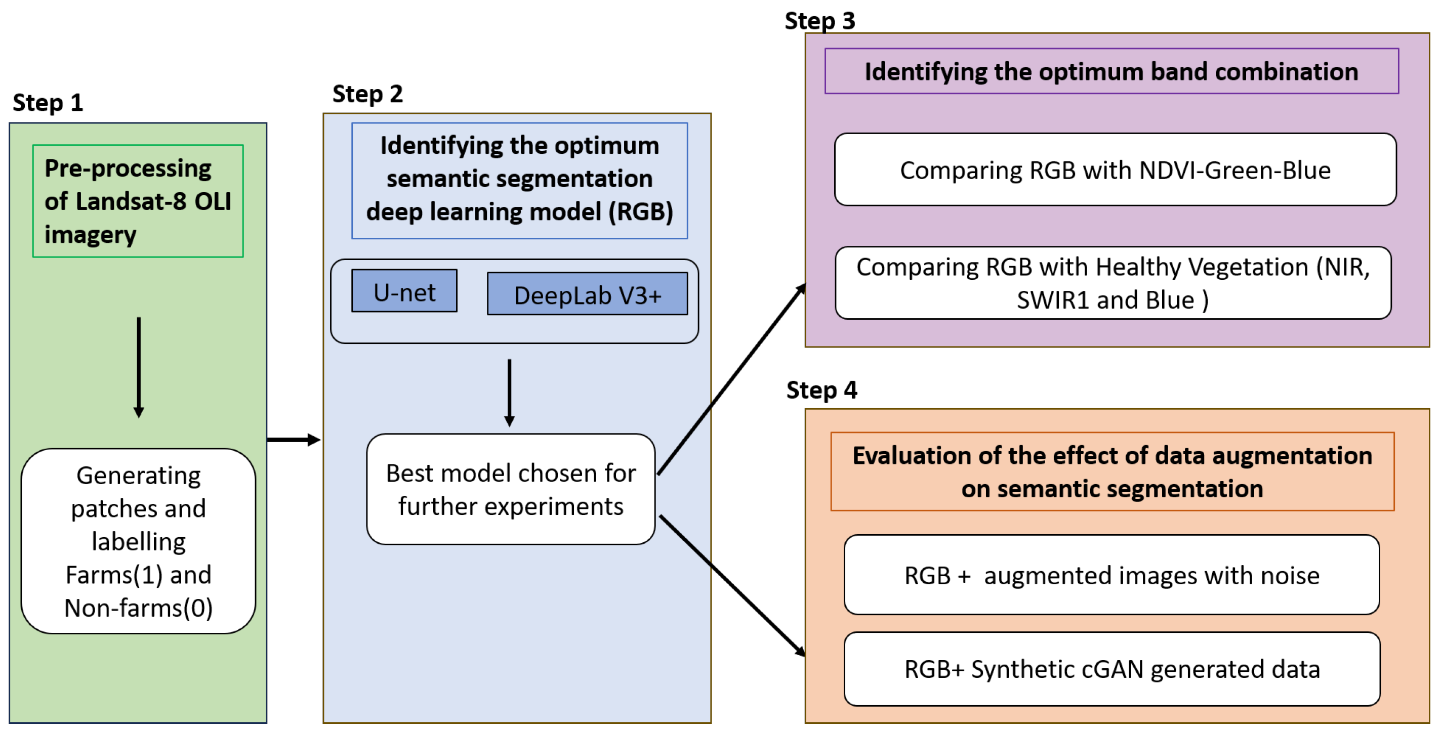
  • We compare two encoder–decoder-based semantic segmentation pipelines using two different convolution strategies.
  • We compare the effects of different band combinations on segmentation results, such as RGB, the normalised vegetation index (NDVI), and the combination of the NDVI and other visible bands.
  • We tackle the problem of label scarcity by data augmentation and generating both images and the masks using a CGAN, in addition to systematically including the augmented images to avoid drastic data shifts in the training samples.
The rest of this paper is structured as follows. Section 2 reviews the relevant literature and describes the necessary background for this study. Section 3 describes the particular study area, the dataset, and the methodology. Section 4 reports the results of the experiments, and, finally, we provide a comprehensive discussion of the experimental results in Section 5.

2. Background and Previous Work

2.1. Farm Area Segmentation in Agricultural Studies

Farm area segmentation is an important step in the analysis of satellite images in agricultural studies, such as crop monitoring. Image segmentation is influenced by different factors, such as the image’s spatial and spectral resolution, the availability of ground-truth labels, the size of the farms, etc. Although farms usually have large land cover features and can be detected even with mid-resolution images, having higher-resolution images would improve the monitoring of crop characteristics and the development of prediction models. That is especially the case in boundary areas, with mixing pixel issues. However, to develop a robust time-series crop prediction model, historical data are essential; thus, despite the growth in a significant number of high-resolution satellite constellations that have been launched recently, they all are fairly new and lack a legacy of data availability, unlike Landsat imagery. The resolution of the Landsat images is 30 m and, with rich, historical, worldwide coverage, which can be used to develop a robust time series-based crop yield prediction model. Due to continuous improvements in the Landsat program and with the upcoming resolution of 10m in the Landsat 9 mission [14], more accurate image segmentation for the monitoring of the crop life cycle would be possible in the future. By addressing these two important factors, i.e., access to historical data and the availability of high-resolution imagery, we can remove important barriers in time-series studies of climate change and allow for more accurate future analyses.

2.2. Traditional Semantic Segmentation Techniques

Before the advent of deep learning models, traditionally, the primitive characteristics of an image were used to perform semantic segmentation. Just as we humans look at an object and learn to differentiate by looking at various features, such as colour, texture, and shape, computer algorithms work similarly. Conventional techniques attempt to find the critical points of an object and define a descriptor for each object. Some examples of such techniques are the scale-invariant feature transform (SIFT) [15], the use of the difference of Gaussian (DoG), and a computationally efficient algorithm named Features from Accelerated Segment Test (FAST) [16] that attempts to find corner descriptors. This group of methods attempts to learn different features, such as an edge, boundary, region, etc. Then, the descriptors can be used for decision-making and object segmentation.
Semantic segmentation methods can be broadly classified into two main categories: supervised and unsupervised semantic segmentation. Supervised semantic segmentation relies on labelled training data to train models that can recognize and segment objects or regions in images. On the other hand, unsupervised semantic segmentation aims to identify meaningful regions or objects without explicit annotations, using data-driven techniques to discover patterns and similarities within the image data. Various techniques are available for segmentation and have distinct characteristics. Threshold-based techniques capture the intensities of neighbouring pixels and assign local threshold values [17]. The Otsu threshold [18] is one of the most widely used standards in different applications [19]. Clustering strategies group pixels into different classes based on different types of visual or spectral features and assign them to separate regions. For example, the Simple Linear Iterative Clustering (SLIC) algorithm [20] clusters pixels based on similarity. Fuzzy C-means [21] provide soft clustering and handle noise well, but they may struggle with sharp boundaries and require careful initialization. Similarly, graph-cut algorithms require the definition of an energy function to incorporate colour and spatial information [22]. On the other hand, there are more recent models based on deep learning methods such as REDO [23], which is based on the scene decomposition concept. It combines dilated convolutions and residual connections for multi-scale context analysis. Their incurred computational cost and complexity are higher. Furthermore, WNET is based on two UNET architectures, which are based on reconstruction loss and a graph-cut loss to avoid over-segmentation [24]. However, the accuracy of the unsupervised methods is usually lower compared to the supervised strategies.

2.3. Deep Learning Strategies in Remote Sensing

Supervised methods, such as conditional random fields (CRF), incorporate spatial coherence and contextual information by modelling dependencies between neighbouring pixels [25], ensuring smoothness in segmentation results. However, CRF may require handcrafted features and additional processing steps, such as feature extraction, data preparation, or parameter tuning, which can introduce complexity and additional time to the overall segmentation process. Then, it can be computationally expensive, particularly for large images. Mask R-CNN combines object detection with instance-level segmentation, delivering accurate and detailed segmentation, yet it is computationally intensive during training and necessitates a substantial amount of labelled training data for optimal performance [26]. U-Net, DeepLab [27], and Transformers [28] are three recent popular models for semantic segmentation tasks. U-Net is an encoder–decoder architecture with skip connections, enabling it to capture both local and global context information. It excels at handling small objects but may suffer from a limited receptive field. Its loss function often includes pixel-wise cross-entropy and dice loss, which can effectively address the class imbalance. However, U-Net may struggle with complex boundary delineation and large dataset requirements compared to Mask R-CNN. On the other hand, the DeepLab family of models utilizes atrous convolutions (dilated convolutions) to enlarge the receptive field, enabling it to capture extensive context information. It may employ various loss functions, such as cross-entropy, Lovász-Softmax, or bootstrapped cross-entropy, which handle object boundaries better than U-Net. DeepLab performs well with large datasets but may not be as effective with smaller ones. In contrast, the Transformer model, originally designed for natural language processing, can be adapted to semantic segmentation using self-attention mechanisms. This allows it to capture long-range dependencies effectively. It often employs the Dice loss function or a combination of cross-entropy and Dice loss. Transformers excel in handling long-range context but may struggle with fine-grained details, leading to less precise segmentation results. They also require substantial computational resources and may not be well-suited for real-time applications.
Many of the above-mentioned methods have been adopted for the segmentation of objects in satellite images. In the case of agricultural fields, the segmentation is influenced by spatial and spectral resolution, the type of bands, labels, farm size and nature of the farm patterns, and environmental conditions such as cloud coverage and illuminations.
For example, the intensity of light in satellite images varies greatly depending on the time of the year and day and weather conditions. Segmentation in such a dynamic scenario is not easy. Although some work has been done [29,30] to alleviate this challenge, overall, traditional algorithms fail to develop models with high generalization for complex field structures and seasonal illumination. In particular, the traditional semantic segmentation techniques have numerous disadvantages as compared to deep learning-based architectures, including lower accuracy and limited ability to handle complex images with multiple objects or overlapping regions. Traditional techniques fail to capture the full context of an image, whereas convolutional architectures learn stronger features with abstraction from raw data [31,32].
Supervised deep learning strategies have been widely adopted in the field of remote sensing for semantic segmentation and have outperformed the traditional methods in various applications, ranging from pre-processing to segmentation and object detection [33]. However, the performance of the models relies heavily on good ground-truth labels to make meaningful predictions. The most common satellites, such as Landsat and Sentinel2, provide visible, NIR, and SWIR wavelengths, allowing for the utilization of different standard wavelengths and combinations thereof. Since satellite images are usually complex based on the diversity of land cover types, including various spectral bands would provide additional information depending on the nature of the desired land cover, such as texture, colour, temperature, water content, and other physio-chemical characteristics. Besides the original bands, a combination of them based on vegetation indices such as the normalised vegetation index (NDVI) has been used for satellite image segmentation. Several works [34,35,36,37] have utilised various band combinations to identify crops and to categorise land use.

2.4. Addressing Data Scarcity and Quality

Another important factor, especially in the case of supervised segmentation strategies, is the amount of training data. Given the challenges in labelling satellite imagery, insufficient training labels are usually a challenge. Reviewing the literature [38,39,40] shows that image augmentation methods have been used to alleviate this problem. Augmentation methods that incorporate geometric transformations and image quality corruption have been demonstrated to enhance the model’s accuracy by effectively expanding the dataset size. Another recent approach to this problem of data scarcity is to generate synthetic imagery using generative adversarial networks (GANs). In [41], GANs were used to perform style transfer on remote sensing images to change the content and meaning of the images. The work transferred styles in between seasons to produce images and different land cover types using the pix2pix [42] GAN architecture. Marin et al. proposed a new network to generate satellite images from available ground-truth labels [43]. GANs are also heavily used to remove clouds in satellite imagery [44].

3. Data Description and Pre-Processing

3.1. Study Area: Emilia-Romagna, Italy

The region of Emilia-Romagna, located in northern Italy (Figure 1), is one of the country’s most advanced regions in terms of agricultural production. The region covers an area of 22,446 sq. km. It benefits from favourable geographical, land and climatic conditions, allowing for the cultivation of a diverse range of crops. Wheat and sugar beets are the major crops grown in this region, together with other vegetables. The region enjoys a mild continental climate year-round, with January being the coldest month, when the temperature drops to 6 °C, and the hottest temperatures are usually recorded in July, at around 30 °C. Rainfall in the region is fairly evenly and distributed throughout the year, with two peak rainfall seasons in the spring and autumn [45]. We selected this region as our region of interest for this study as it has a good spread of farmlands [46], which are clear enough to be segmented in 30 m resolution satellite images.

3.2. Experimental Data

The Earth observation satellite mission called Landsat 8 was launched and operated jointly by NASA and the United States Geological Survey (USGS) in 2013. The mission consists of two major sensors divided into different band ranges, and a total of 11 bands are available. The satellite is capable of operating in near-infrared and visible light to thermal infrared bands.Each band is categorised by different wavelengths. Operational Land Imager (OLI) and the Thermal Infrared Sensor (TIRS) are the two main instruments responsible for providing earth coverage at 30 m resolution for visible, infrared, and near-infrared light—100 m for thermal and 15 m for panchromatic. Landsat 8 captures at an interval of 16-day frequency, with 740 daily scenes [47]. In the context of Landsat images, a “scene” refers to a specific area on Earth’s surface that is captured by a single sweep of a Landsat satellite. These scenes are organized and indexed according to the Worldwide Reference System to make it easy to locate and access images of particular regions. Table 1 describes the different band information.
Satellite imagery from Landsat OLI 8 Collection 2 Level-2 covers the region of interest (ROI) in two tiles/scenes as seen in Figure 2. Landsat OLI 8 scenes from Emilia-Romagna (44.5968°N, 11.2186°E), for July 2020, with less than 10% cloud coverage, were used for this study and were downloaded from EarthExplorer [47], out of which it was ensured that only cloud-free, clear image tiles were selected after generating patches.

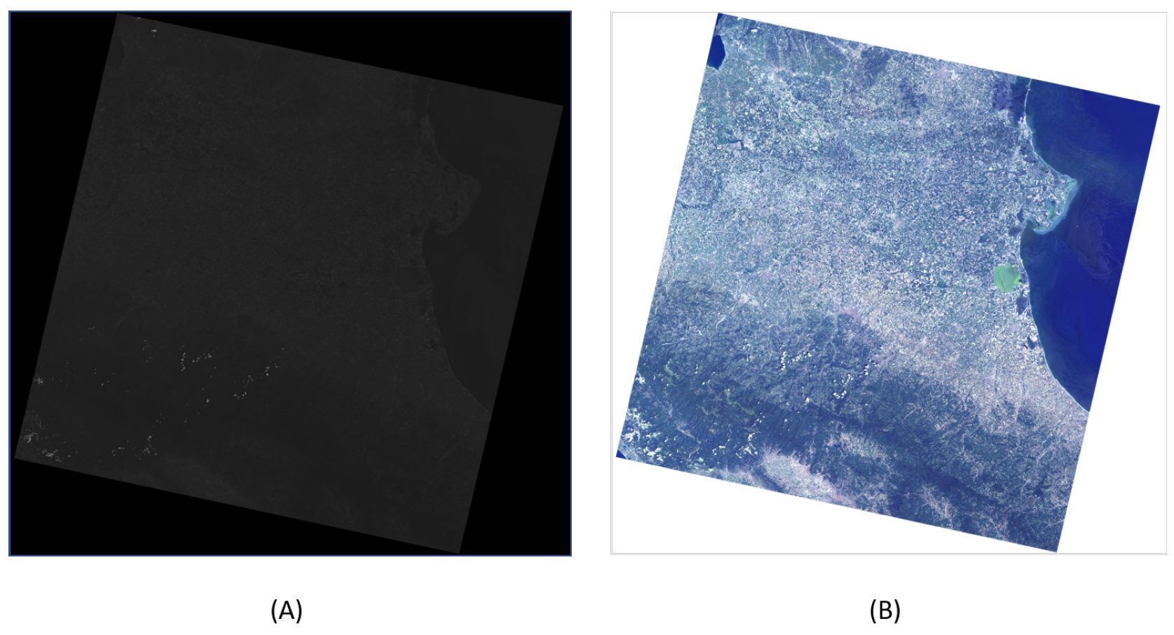
3.3. Satellite Imagery Pre-Processing

3.3.1. Radiometric Band Correction

Radiometric band correction eliminates the effects of atmospheric, illumination, and other errors incurred by the sensors to enhance the quality of satellite imagery. The corrections are applied by first converting the digital number to spectral radiance, and then into reflectance. To make the satellite images ready for analysis/experiments, certain pre-processing steps need to be implemented. Some of the most commonly followed steps are conversion to radiance, solar correction, atmospheric correction, topographic correction etc. [48]. The Landsat 8 imagery is radiometrically corrected, and more on these corrections can be learned in detail from the Landsat 8 handbook [49].
In this study, the image tile downloaded from Landsat OLI 8 consists of various bands mentioned in Table 1 in the GeoTIFF format. They are available as 16-bit images with unique multi-spectral bands at 30 m resolution. Combinations of these bands, when used in varying configurations, result in composite images. For example, the band combination (4, 2, 3) yields a natural composite image [50].

3.3.2. Dark Object Correction (DOC)

Dark object correction (DOC) is a pre-processing technique commonly used in remote sensing and image processing to mitigate the effects of atmospheric scattering in satellite or aerial images (Figure 3). It involves identifying dark objects in the image, such as bodies of water or regions with low reflectance, which are assumed to represent areas with minimal contribution from surface features. By using these dark objects, the technique estimates the contribution of atmospheric scattering. The estimated scattering values are then subtracted from the original image values, resulting in a corrected image that reveals more accurate information about the underlying surface features. In some cases, each pixel in the image is subtracted by a reference value, which is typically chosen as the lowest value found in the near-infrared (NIR) band. This reference value serves as a baseline and helps eliminate the impact of haze and atmospheric scattering, further enhancing the clarity of the corrected image [51,52]. All bands were converted to radiance and DOS-corrected using the free free QGIS Desktop 3.22.11 software [53].

4. Methodology

In this work, supervised semantic farmland segmentation is performed using deep neural network-based architectures and pre-trained networks. To improve the performance of the models, we further explore different strategies to increase the accuracy by leveraging the use of different band information. The imagery dataset is also expanded by adding transformations, such as geometric transformation and corruption of pixels by adding noise. Synthetic image generation is widely used in medical fields to expand the limited data, and this paper attempts to generate image and mask pairs using conditional GANs to generate more training samples. The overall experimental analysis followed is described in Figure 4.

4.1. Supervised Semantic Segmentation

Since the main aim of this current study is farm area segmentation, everything other than farmlands is considered as the non-farm category. The farms are labelled as 1 and non-farms as 0. To generate training patches of an image, the tile was divided into patches of size 256 × 256 as illustrated in Figure 5. In the following, the two main segmentation strategies employed in this study will be explained briefly.

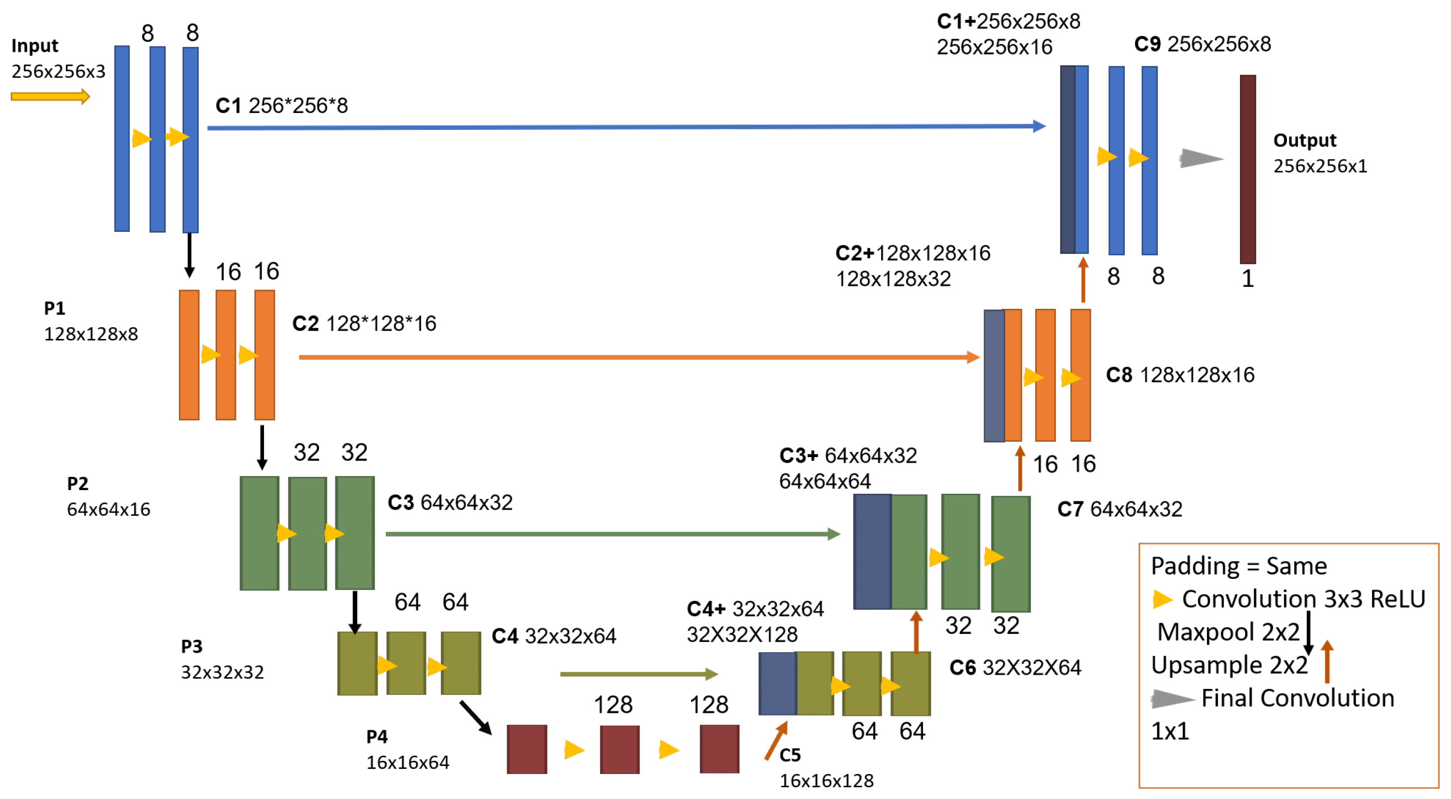
4.1.1. Multi-Scale Feature Fusion Based on U-Net

In a deep learning architecture, the higher-level features extracted at deeper layers hold more information about the semantics but fail to capture the spatial details due to stride convolutions and pooling. It is essential for the lower-layer features and the features extracted at deeper levels to work together to boost the performance of the model. Fully convolutional networks (FCNs) [54] introduced feature enhancement techniques by using the skip connection strategy. The feature for prediction and the features located in the middle layers are connected via a skip connection. This strategy has improved semantic accuracy. Rooneberger et al. [12] proposed the U-Net architecture in 2015 for biomedical image segmentation. The architecture (Figure 6) is an encoder–decoder, which extracts the features from each layer by using skip connections. The encoder acts as the contraction path, learning the latent representation of the input image. It reduces the spatial dimension and doubles the number of feature channels at every encoder block, whereas, at the opposite end of the architecture, the decoder acts as the expansion path, retrieving the compressed information by doubling the spatial resolution. The skip connection ensures that the feature maps to the decoder so that it learns better and produces better output.
The U-Net architecture has gained popularity in medical image segmentation and has also found applications in segmenting urban images. By employing a softmax function, the model generates segmentation results that can effectively delineate objects of interest in the input images. What sets U-Net apart from other CNNs is its ability to achieve accurate segmentation with a smaller training dataset. This means that U-Net can effectively identify and label specific regions within an image, resulting in higher precision when compared to alternative CNN architectures [55].

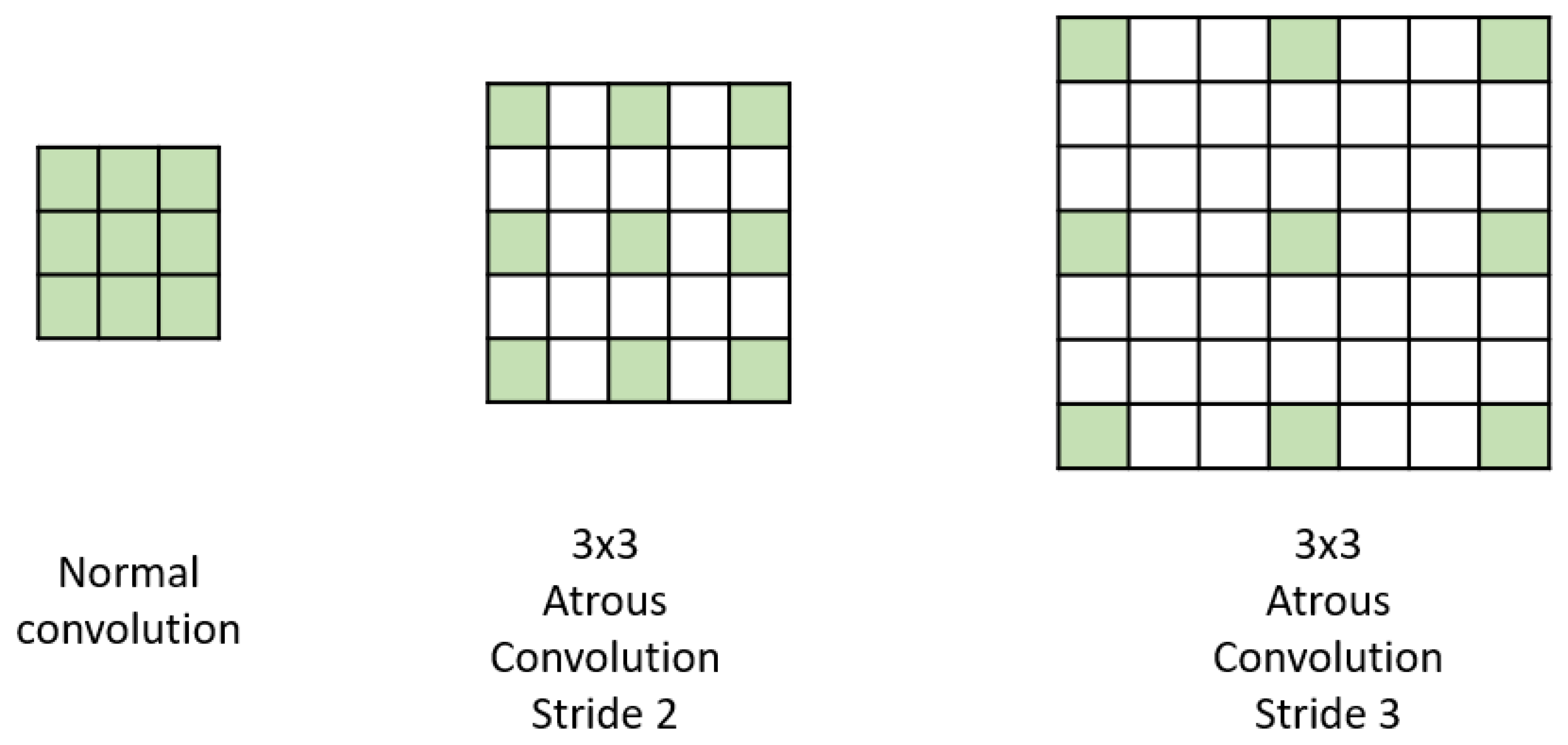
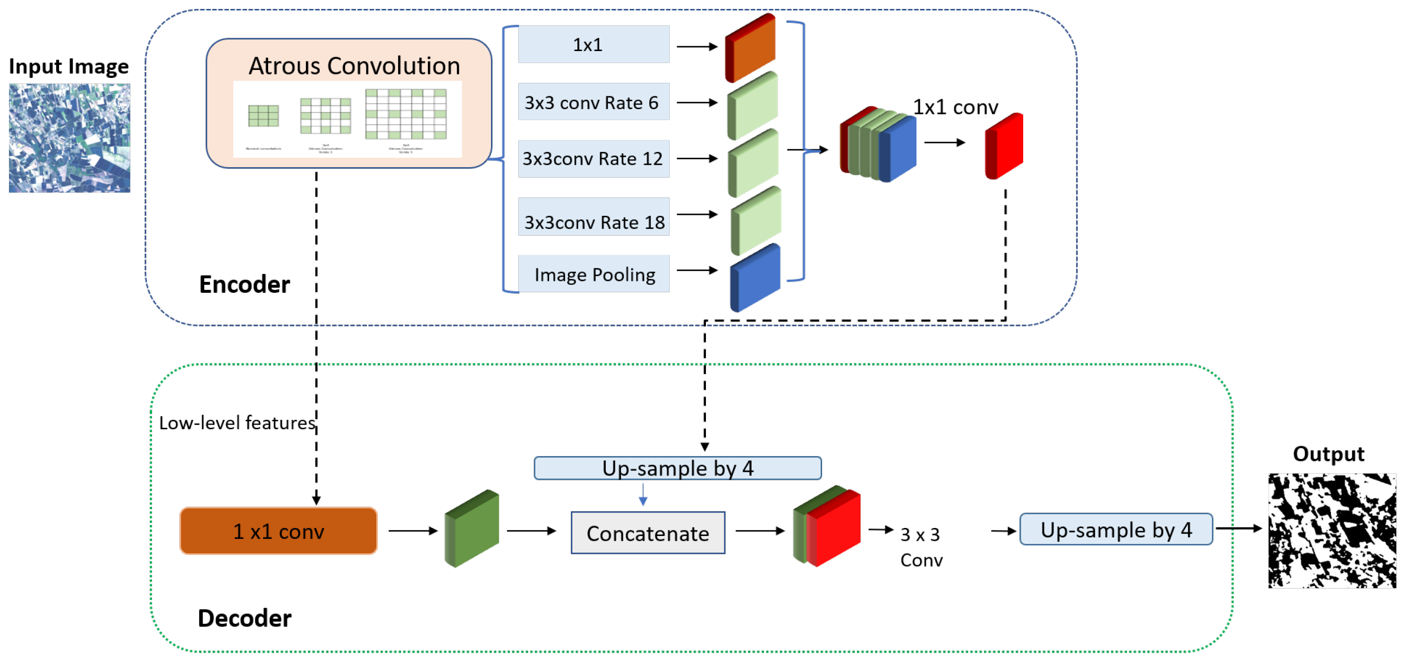
4.1.2. Contextual Features Based on Atrous Filtering

This group of methods looks at the full context of the image to make the model aware of the semantics, not just at the pixel level but at the overall picture/context of the image. Context information can boost the performance of the models. Dilated-Net [56] is one such popular method; by aggregating the different multi-scale contexts on dilated convolution, it leverages the use of dilation rates based on the receptive field. The larger the receptive field, the higher the dilation rate for the convolution. Five different dilation rates, i.e., 1, 2, 4, 8, and 16, are used to derive contexts. A CNN combined with conditional random fields is used to extract the patch-wise context in the multi-scale pyramid pooling module (PPM) [13]. The module has laid the foundation for some very popular methods, such as the DeepLab family [27], which leverages atrous spatial pyramid pooling (ASPP) and replaces the pooling with atrous convolution, as illustrated in Figure 7.
The Deeplab family of models is based on atrous convolutions. DeepLabv3+ as shown in Figure 8 is implemented using the encoder–decoder architecture. It overcomes two problems faced while using fully convolutional network-based algorithms for semantic segmentation; first, it compromises feature resolution by pooling operations and because the objects exist at multiple scales [13]. As the name suggests, the model comprises two parts: the encoder, which is responsible for reducing the feature maps and extracting the semantic features, and the decoder, which recovers the spatial information. The advantage of DeepLabv3+ over its former version, Deeplabv3 [57], is that the encoder bi-linearly upsamples by a factor of 4 instead of 16 to avoid any loss of features and, thereafter, combines with the low-level feature from the encoder with the same spatial resolution. The architecture can be seen in Figure 8 below.
The CNN architecture with integrated atrous convolutions enables the capture of multi-scale contextual information without significantly increasing computation. This is crucial for segmenting farmlands with varying sizes and complexities. The ASPP (atrous spatial pyramid pooling) module in DeeplabV3+ further enhances context aggregation by using multiple parallel atrous convolutional layers with different dilation rates. This enables the model to capture both local and global features, aiding in farmland boundary delineation. Moreover, the skip connections and feature fusion through the decoder part of DeeplabV3+ help refine segmentation maps by combining low-level and high-level features, allowing it to effectively capture intricate details in farmland imagery. In the implemented DeepLabv3+ model, after some initial tests with different stride values, a stride of 16 was found appropriate for the model.

4.2. Spectral Images for Semantic Segmentation

The interaction of electromagnetic energy with the vegetation in different band spaces, such as red, green, blue, and other infrared bands, helps to formulate different indices. In agriculture and environment studies, different indices are used by combining the visible and NIR bands of the satellite images. Transforming multiple spectral bands into one vegetation index allows the farmland or land cover vegetation objects to be better distinguished and enhances segmentation in satellite imagery.

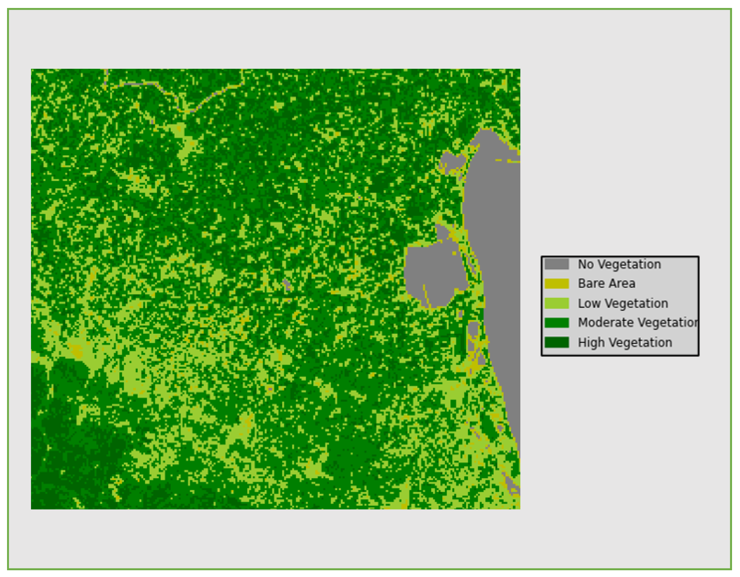
4.2.1. Normalized Difference Vegetation Index (NDVI)

The health of vegetation can be directly estimated using the NDVI [58]. The NDVI is a popular vegetation index due to its ability to provide a direct indication of the health of vegetation. It effectively captures vegetation health by utilizing a normalized difference calculation and focusing on the areas where chlorophyll absorbs and reflects light the most. This characteristic enables NDVI to be highly informative across various conditions. The vegetation can be highlighted using simple thresholds of higher values, removing the other lower reflecting surface materials. The NDVI is calculated as follows:
NDVI = NIR Red NIR + Red ,
The values the range between +1, indicating healthy vegetation, and −1, indicating no/poor vegetation (Figure 9).

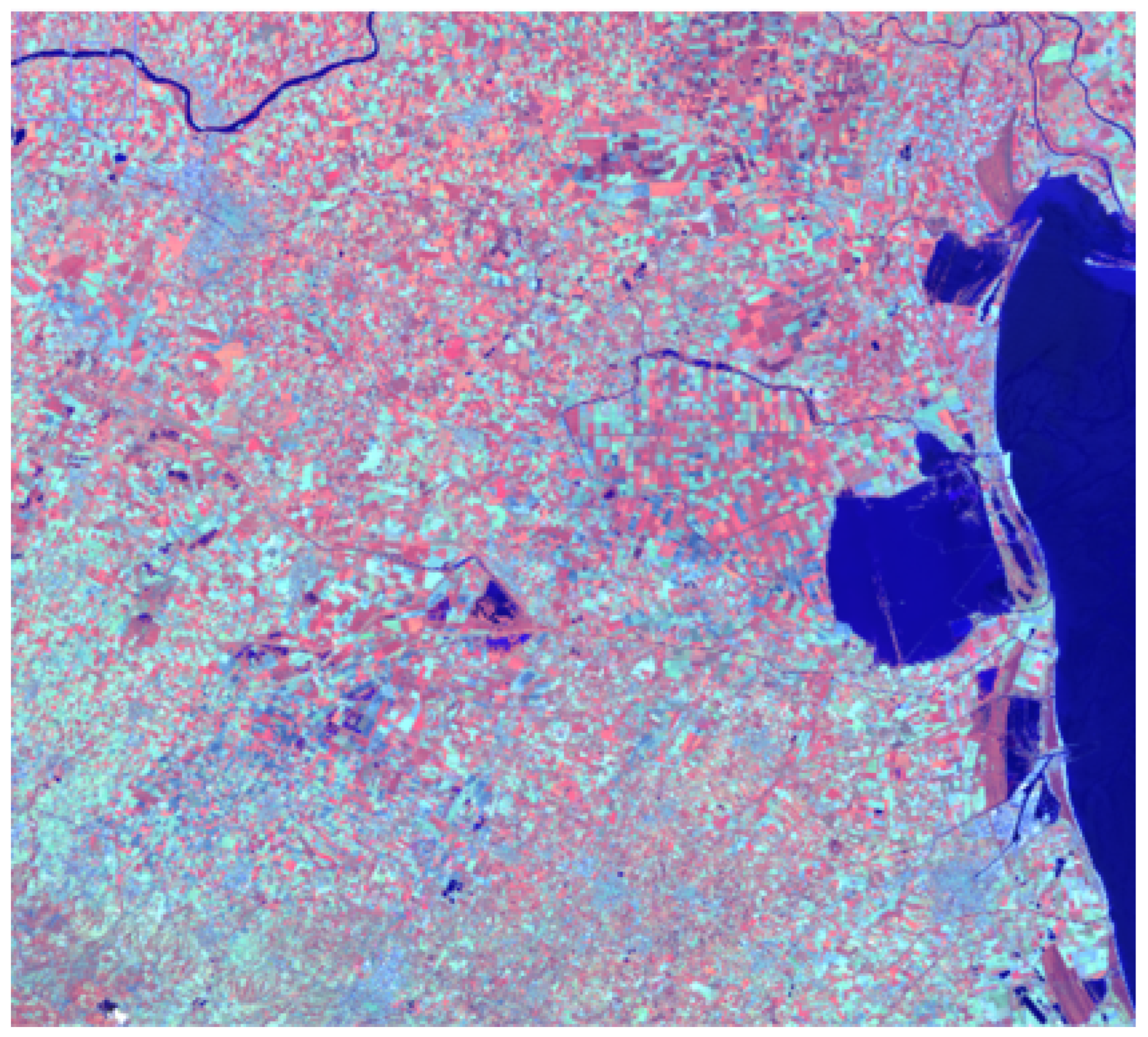
4.2.2. Agriculture Band Composite Imagery

Band combinations of the NIR, SWIR1, and blue ranges are widely used for crop monitoring. As illustrated in Figure 10, land with healthy crops is distinguished by shades of orange, red, and brown, whereas uncultivated areas with soil are black to brown, and other land cover, such as residential areas, is cyan blue [59]. The NIR band’s range indicates the highest plant leaf-based reflectance, making it ideal for crop monitoring.

4.3. Data Augmentation

Image augmentation is essential when there is a scarcity of labels for supervised semantic segmentation. In this context, data augmentation refers to the process of generating new training samples by applying various transformations to the existing labelled images [60,61,62]. This technique effectively increases the diversity and quantity of the available training data, which, in turn, enhances the performance and generalization of the supervised semantic segmentation model. The significance of data augmentation lies in its ability to alleviate the effects of label scarcity. Since obtaining accurate pixel-level annotations for semantic segmentation can be time-consuming and costly, the availability of labelled images is often limited. However, by augmenting the existing labelled data, new samples can be generated based on two main strategies. (i) Image corruption and transformation, such as rotation, adding noise, and pixel distortion, can be employed. This only expands the number of images, but no new labels are generated. (ii) A data-driven strategy based on GANs can also be used. To generate new images, as well as labels, a CGAN can be used. This artificially expands the training dataset, allowing the model to learn more robust and discriminate features, improving its ability to handle diverse real-world scenarios.
Nevertheless, there is a risk associated with augmenting data excessively. When data augmentation is applied excessively, it may lead to over-fitting [62,63,64]. Data augmentation can also introduce model shift problems. Model shift refers to the phenomenon where the performance of a model deteriorates when it is exposed to data that significantly differ from the training distribution. If the augmentation techniques used during training do not adequately represent the real-world variations in the test data, the model may struggle to accurately segment the unseen images. This can result in a significant drop in performance when deploying the model in real-world scenarios. To mitigate these risks, it is crucial to strike a balance between the amount of data augmentation applied and the diversity of the augmented samples. One of the challenges encountered in the analysis of readily available satellite images lies in the absence of structured and labelled datasets, which is particularly true for developing countries. Consequently, preparing a substantial dataset of labelled imagery for the specified area presents a formidable challenge. To enhance the existing datasets for deep learning models, the adoption of data augmentation techniques becomes imperative. This paper aims to elucidate the two augmentation methods, one encompassing various strategies such as image transformations and corruption and the other by generating images using CGANs.

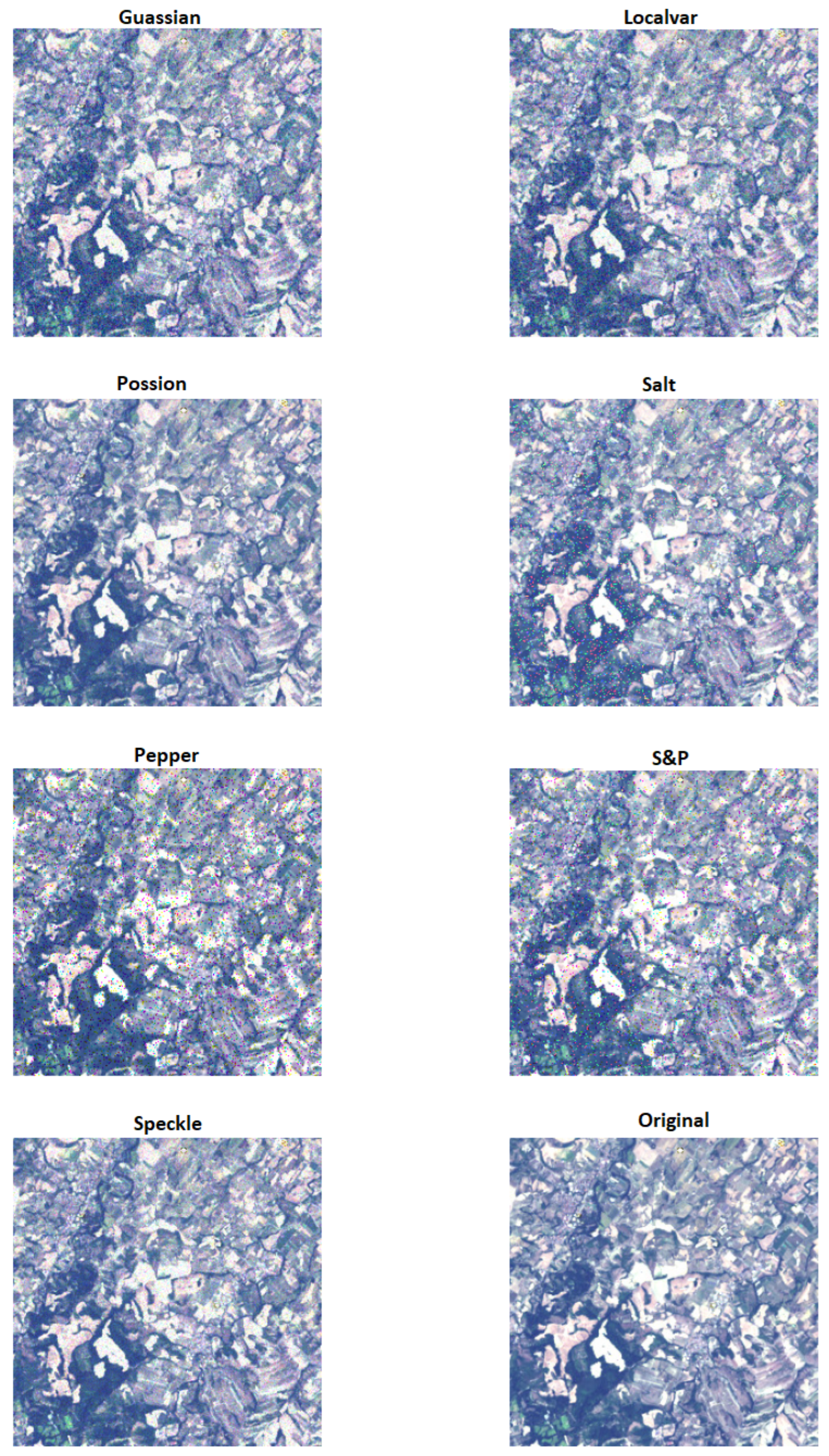
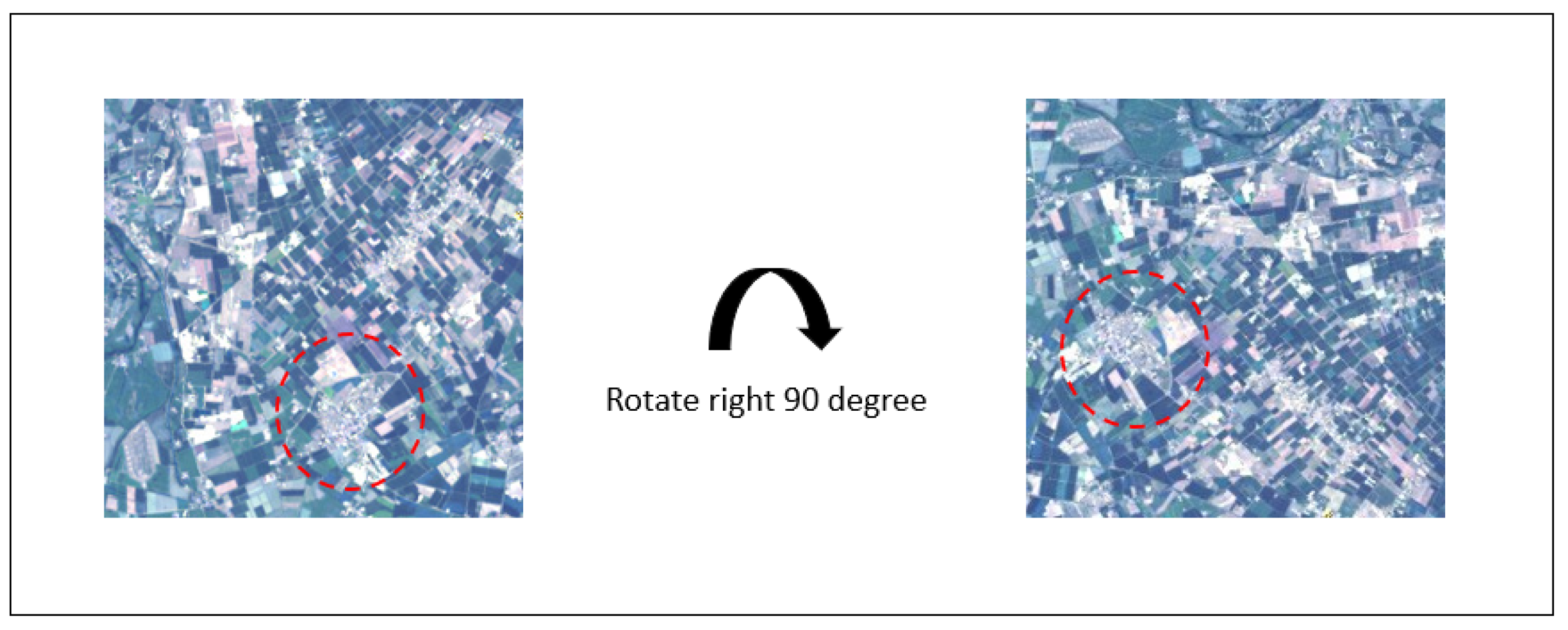
4.3.1. Image Augmentation Based on Transformation and Noise

In order to increase the training samples, we experimented by injecting noise into the dataset to expand the existing imagery. As seen in Figure 11, different noises, such as Gaussian, salt, pepper, a combination of salt and pepper, local var, speckle, and Poisson, were added. To add geometric transformation, the images were rotated 90 degrees to the right, as illustrated in Figure 12 below.
We used the free Python image processing toolbox scikit-image [65]. The probability of noise was set to 0.05 to avoid any major deterioration of pixels.

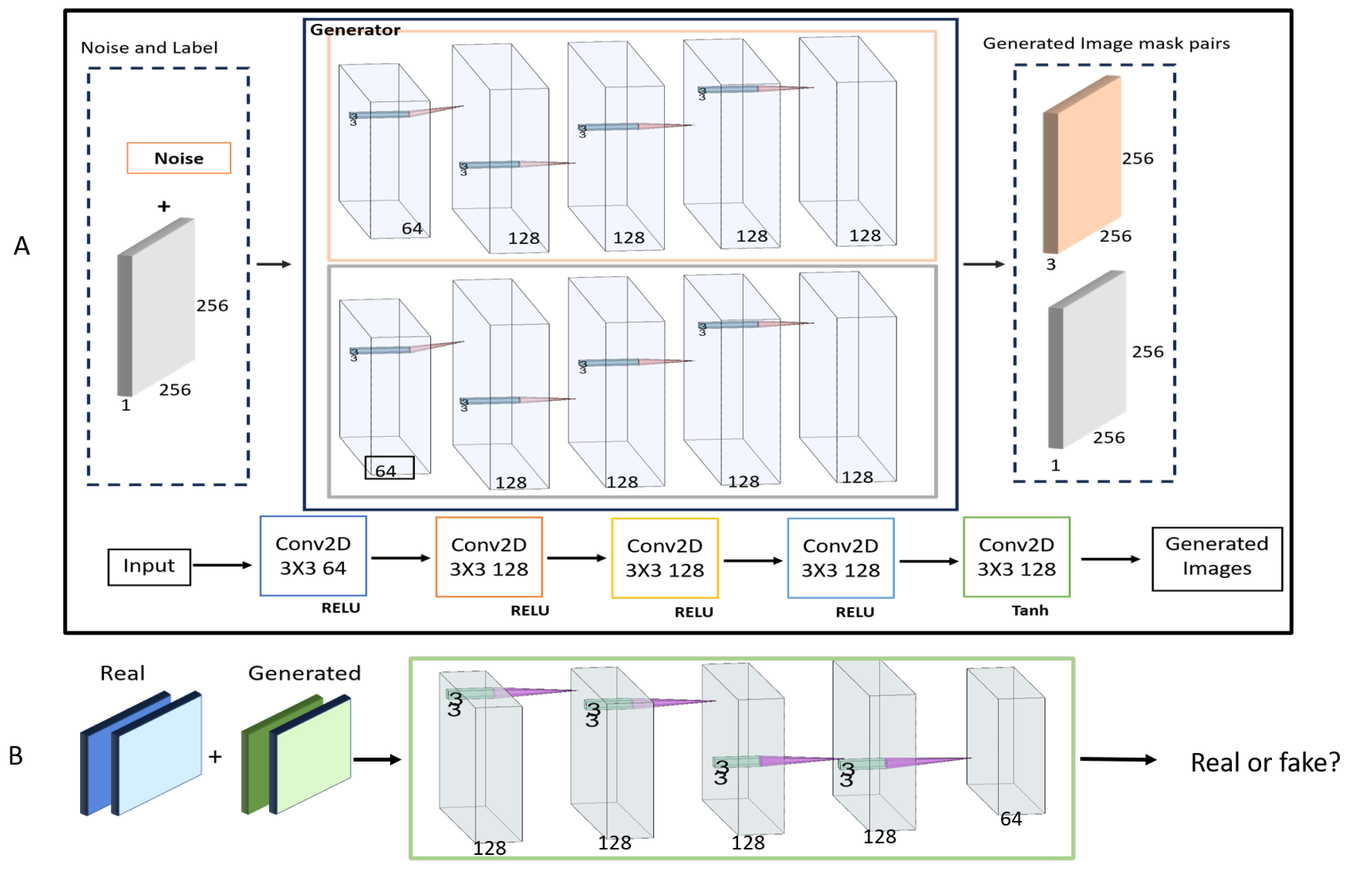
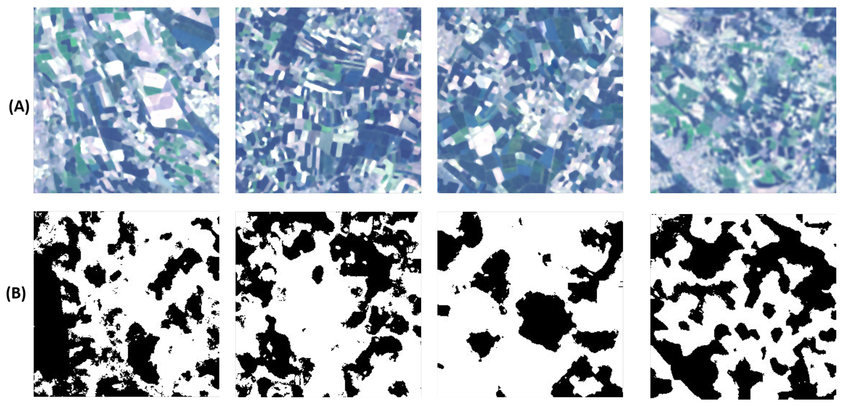
4.3.2. Conditional Generative Adversarial Models (cGANs) for Data Augmentation

A generative adversarial network (GAN) is a generative model consisting of two main components: the generator and the discriminator. The role of the generator is to produce new images from given training samples such that the discriminator is not able to discriminate them from real samples. ‘Adversarial’ indicates that the training is conducted simultaneously in a zero-sum fashion, i.e., the better the discriminator performs, the worse the performance of the generator and vice-versa if the discriminator fails to identify real or fake (generated) images. They compete against each other, and eventually, both components improve together. In 2014, conditional GANs were developed to achieve the controlled generation of synthetic images [11]. The generator and discriminator are provided with additional information about the images in the form of ‘labels’. The coupled loss function of the network is described in the following equation:
m i n G m a x D V ( D , G ) = E x [ l o g D ( x | y ) ] + E z [ l o g ( 1 D ( G ( z | y ) ) ) ] ,
where D(x|y) represents the discriminator’s probability of guessing that x is real, given the condition/label y, whereas E x is the expected value for all real data. G(z) is the output generated by the generator given noise z. D(G(z|y)) is the discriminator’s prediction that the fake sample is real. E z signifies the average value we expect to obtain from the generated fake instances when considering all potential inputs.
In our work, the limited dataset is expanded using conditional GANs for the generation of synthetic images and mask pairs. To implement this, we adapted the method proposed in the works of Neff et al. [66], which was originally developed for medical image segmentation using a DCGAN [67]. In this study, we adopt a modified, diagrammatically represented in Figure 13 CGAN model [66]. The original work was developed for X-ray images, to generate synthetic image-mask pairs. However, there are differences between the satellite imagery data and the previous work on medical X-ray images in terms of their texture, pattern distribution, and resolution. Satellite images consist of diverse textures and distributions of patterns due to the wide range of the viewed land covers and environmental factors, e.g., weather conditions. Another challenge is that there is not necessarily a balanced number of pixels from all land cover types in the view of satellite images. Moreover, their lower resolution (1 pixel = 30 m) due to the far view of the sensor poses challenges for accurate synthetic image generation. Thus, the heterogeneous patterns in satellite imagery require the capture of diverse features and the learning of a greater number of data distributions by the generator of the CGAN model. That is more challenging using adversarial loss in a CGAN compared to the more homogenous classes of patterns in medical X-ray images. Although the adopted CGAN pipeline parameters were optimized for the remote sensing data, the effect of the induced challenges as described causes challenges in reaching convergence in adversarial training and influences the images synthesized by the model generator that attempts to convincingly mimic real-world scenes. Therefore, two further experiments were conducted for the evaluation of the synthesized images in terms of sharpness and color, which will be described in the following sections.
The model architecture includes a generator that is divided into two channels, as shown in Figure 14: one for the image and the other for the mask. This is forwarded to the discriminator, which, now, instead of classifying a single image, takes into consideration an image–mask pair for classification (for more details, refer to the implementation reported in [66]). The input data were re-scaled to fall within the [−1, 1] range, and an Adam optimizer [68] was employed, utilizing a learning rate of 0.0002. A batch size of 128 was deployed to generate samples. RELU [69] was in all layers of the generator, except for the output layer, where the hyperbolic tangent (tanh) activation function was used. The discriminator, on the other hand, used LeakyRELU [70] to allow values less than zero and performs better than using RELU [71].
Mode collapse, as described in reference [72], refers to a situation in which the generator acquires the ability to associate multiple distinct noise vectors (inputted as z) with a single resulting image (G(z)). In our work, the ‘farm’ class dominates the dataset; thus, the generated population majorly comprises farms. To tackle this phenomenon to a certain extent, we evaluated and chose a good mix of variety (including ‘farms’ and ‘non-farms’) as input to the GAN architecture. The generated images and masks exhibit a remarkable similarity to the training population. However, some slight blurriness is noticeable in the generated images, as illustrated in Figure 15. This blurriness can be attributed to limitations in the generator’s ability to accurately capture the edges and subtle characteristics of the minority class, as well as sudden changes in objects within the images [73].
To measure the significance of the deviation of the generated images from the original training samples, they are compared in terms of sharpness and colour. For the former, the Laplacian variation of the two image populations is calculated. The Laplacian captures the sudden changes in intensities and is therefore capable of identifying the edges in an image. If the variance of the Laplacian-applied image is low, it indicates low responses due to a lower number of edges. The blurrier the image, the fewer edges and vice-versa for a clear image. The Laplacian is a second-derivative operator that is used for image edge detection. Given an image array (f), this operator is defined as follows:
f = 2 f = 2 f x 2 + 2 f y 2
where x corresponds to columns (width) and y corresponds to rows (height) of the image array.
The Wilcoxon p value was used to compute statistical the significance of the deviation between the sharpness of the two image groups. Furthermore, the colour histogram of the two groups was considered to check their colour deviations.

4.3.3. The Proposed Augmentation Strategy

The limited labelled RGB imagery dataset was augmented by introducing various types of noise, as explained in the above sections. The noise was applied to the input images to create additional variations, thereby expanding the dataset. This augmentation technique aims to increase the model’s robustness to noise and improve generalization by exposing it to a wider range of training examples. Secondly, to mitigate potential data shift issues caused by introducing synthetic data, we incorporated the synthetic data in small batches during training. This approach prevents major discrepancies between the synthetic and real data distributions and reduces the likelihood of over-fitting or biased model behaviour. By introducing the synthetic data gradually, the model can adapt and learn from both the real and synthetic data sources.

4.4. Evaluation Metrics

4.4.1. Pixel Accuracy

As the name suggests, pixel accuracy is the number of pixels correctly predicted as compared to the ground-truth labels. High pixel accuracy alone does not indicate that the model is accurate; it is therefore cross-checked with other metrics, such as MIoU, as explained in the following section.
P i x e l A c c u r a c y ( P A ) = T P + T N T P + F N + T N + F P

4.4.2. Intersection over Union (IoU)

Intersection over union overcomes the partiality of accuracy in semantic segmentation, especially for problems where there exists class imbalance. IoU uses a fraction of the intersection/overlapping area to the union between predicted labels and the ground-truth labels. Absolute overlap between the union and intersection indicates perfect overlap and yields 1 for the highest score and 0 for no overlap in segmented areas compared to the true labels. In binary and multi-class cases, the mean of the IoU (MIoU) for each is calculated,
I o U = T r u e p o s i t i v e s ( T P ) T r u e p o s i t i v e s ( T P ) + F a l s e p o s i t i v e s ( F P ) + F a l s e N e g a t i v e s ( F N )

4.4.3. Matthew’s Correlation Coefficient (MCC)

MCC was first developed to study chemical structures and was later leveraged as a metric in machine learning models [74]. MCC gives equal importance to both the positive- and the negative-class prediction of a dataset. The values range between −1 and 1, where 1 indicates exact prediction as ground-truth labels and −1 denotes other cases. It strikes a balance between all four values in a confusion matrix (6), giving a score based on the output for both classes. It is formulated as shown in Equation (6) below.
MCC = T P · T N F P · F N ( T P + F P ) · ( T P + F N ) · ( T N + F P ) · ( T N + F N )
Regarding the importance of these three metrics, pixel accuracy measures the overall proportion of correctly classified pixels; however, it does not account for class imbalance or error types; thus, when classes are imbalanced, relying solely on this metric can lead to misleading conclusions. MCC considers the true positives (TPs), true negatives (TNs), false positives (FPs), and false negatives (FNs), providing a balanced measure of performance, especially for data with class imbalance cases. In this paper, the dataset is skewed towards the farm class, accounting for more than 60% of the pixels. IoU shows the success of the model in segmenting the boundaries of the class of interest (farms in this study) compared to the wrongly segmented boundaries in both the positive-class (FP) and negative-class (FN) sides. Therefore, it is valuable for tasks with precise object boundary localization.
Therefore, in this study, we employed all three metrics to better gauge the performances of the models. When they are not consistently agreed upon, the methods showing success in most metrics can be considered. Then, in some cases, appropriate post-processing techniques can be employed to further refine the segmentation results in parts connected to the less successful metrics. For example the small gaps among large, segmented farms could be filled at a post-processing stage.

5. Results

The segmentation models were trained using PyTorch 1.10. The train–test split was fixed at 70–30% for all the experiments. The data used for training and testing were selected at random from the available image patches. We employed a random sampling process to mitigate the risk of any unintentional data leakage between these sets. There are no overlaps between the training and testing sets.

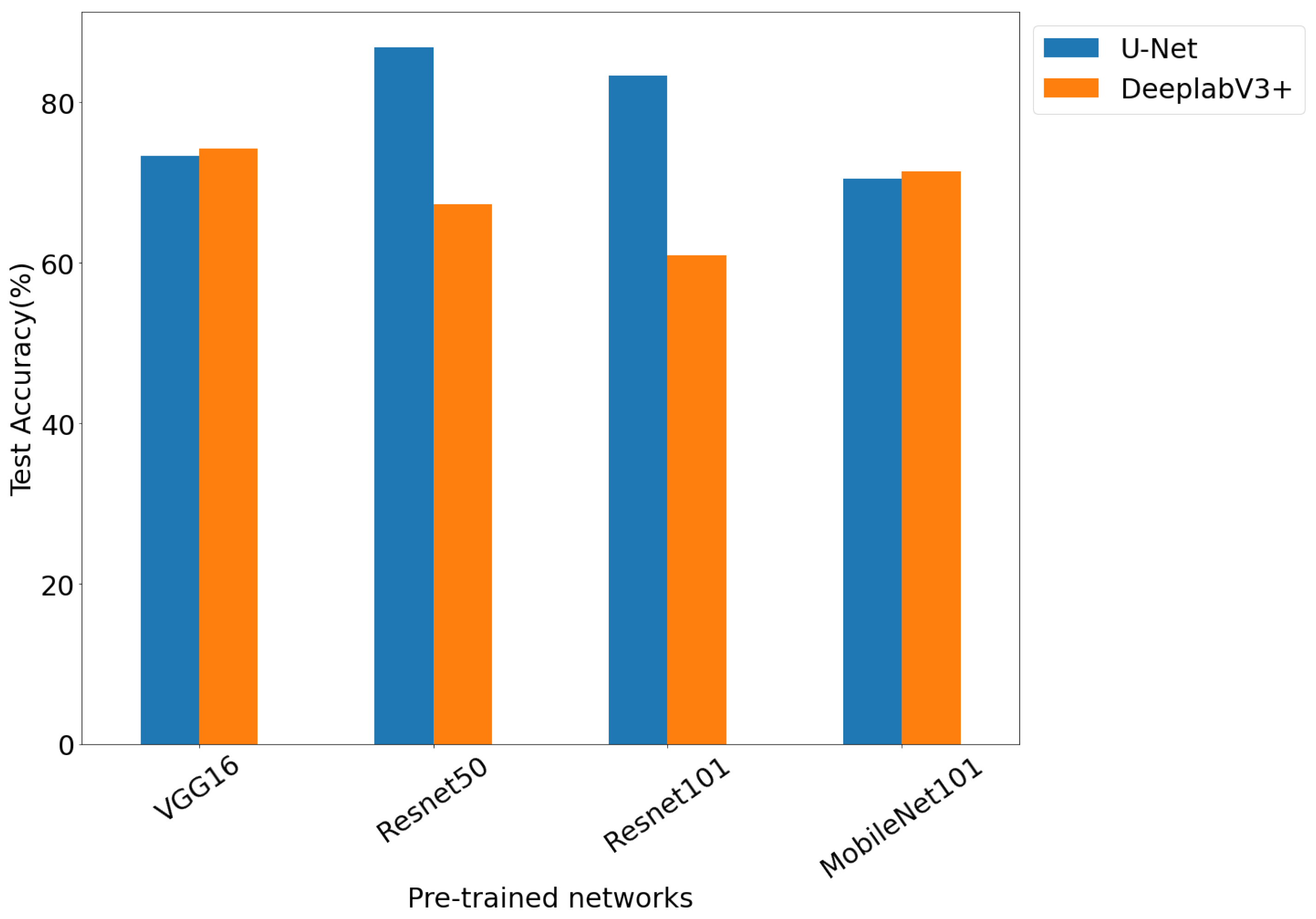
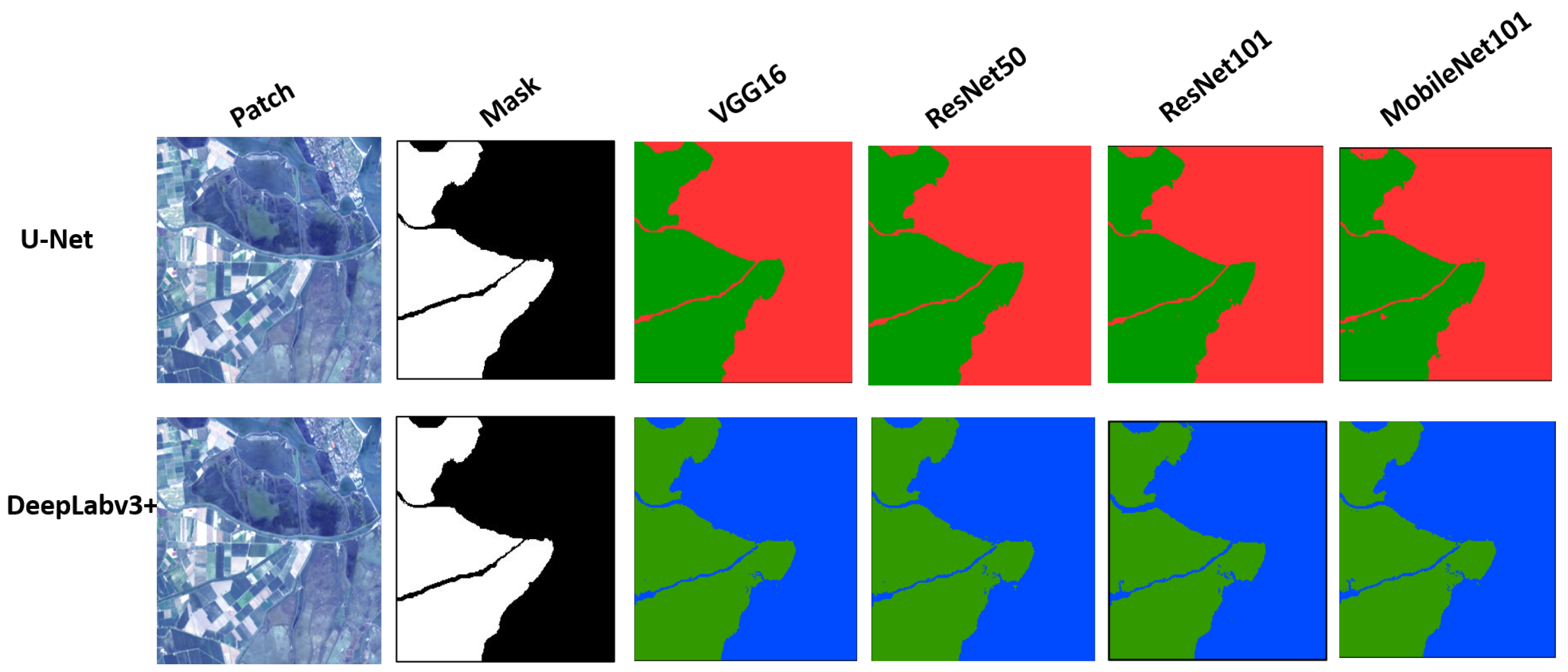
5.1. Supervised Semantic Segmentation

The first set of experiments is based on the utilization of the original training of RGB images, where the two selected segmentation modelling strategies, U-Net and Deeplabv3+, were compared. The U-Net model performed comparatively better with transfer learning strategies on a small dataset as compared to Deeplabv3+. U-Net achieved the highest overall MIoU score of 83.12. Overall, the Resnet model outperformed the other models and provided results consistent with those of the U-Net architecture for all three metrics. The results are summarized in Table 2 and Table 3 below.
As seen in Table 3, we learn that despite the atrous spatial pyramid pooling networks in the Deeplabv3+ models, the results are relatively low as compared to the U-Net models. These results show that the role of the mid-level features carried via the skip connection in the U-Net architecture are more important than the atrous filtering in the DeepLabv3+ model. That might be connected to the texture type of the farms in the satellite images. Since the algorithm attempts to find all different farms with diverse kinds of crops as one class, the non-farm class is also very heterogeneous. Therefore, different levels of features contribute better to discrimination as compared to multi-scale features. It is also reported that the latter method works better for the segmentation of a single large object in high-resolution images [75]. However, the Landsat images are not in high resolution, and farms are not necessarily the most extensive land cover type in all patches of images used in this work. All three metrics agree in terms of the achievement of the best results using the VGG16 model.
The performance difference between U-net and DeeplabV3+ can be observed in Figure 16 below.
It is worth noting that, for the training of deeper convolutional models, a higher number of training samples is required compared to shallower models. Although we performed transfer learning on the previously trained models, fine–tuning based on the existing labelled data was conducted. Then, as the models grow deeper, they tend to fail to generalize well on new satellite images and perform comparatively less accurately. Hence, considering the limited availability of satellite RGB images with 30-m resolutions, ResNet50 and VGG16 outperformed the deeper models, like ResNet101 and MobileNetV2, due to their less complex architectures and lower numbers of parameters. The reduction in model depth also reduced the risk of over-fitting, allowing the models to capture intricate features effectively rather than memorising the training data to survive. Comparison of the performance of the model trained using RGB images from scratch reported in Table 4 with the results of the pre-trained models reported in Table 2 and Table 3 shows a similar range of results, with a slight drop in a few cases supporting this. Figure 17 shows the best model result from Table 2.
On the other hand, none of the pre-trained models was developed based on spectral satellite images, and we could only use the RGB bands to match the input requirements of the pre-trained models. That also influences the success of the models, since the NIR bands are correlated with the chemical characteristics of the objects and play an important role in the detection of land cover in the remote sensing domain. For this reason, we performed segmentation using different combinations of the visible and other NIR and IR bands, which will be presented in the following section. In this paper, when building a model from scratch using other wavelengths, a systematic search from shallower to deeper architecture was conducted, and once the models started to over-fit, the depth was kept fixed, and no further layers were added.

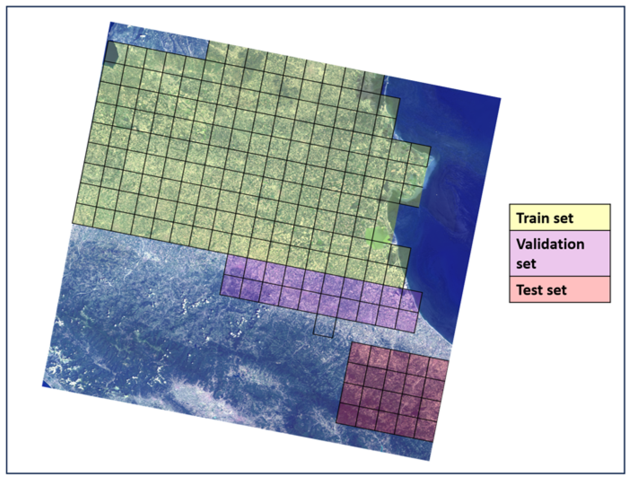
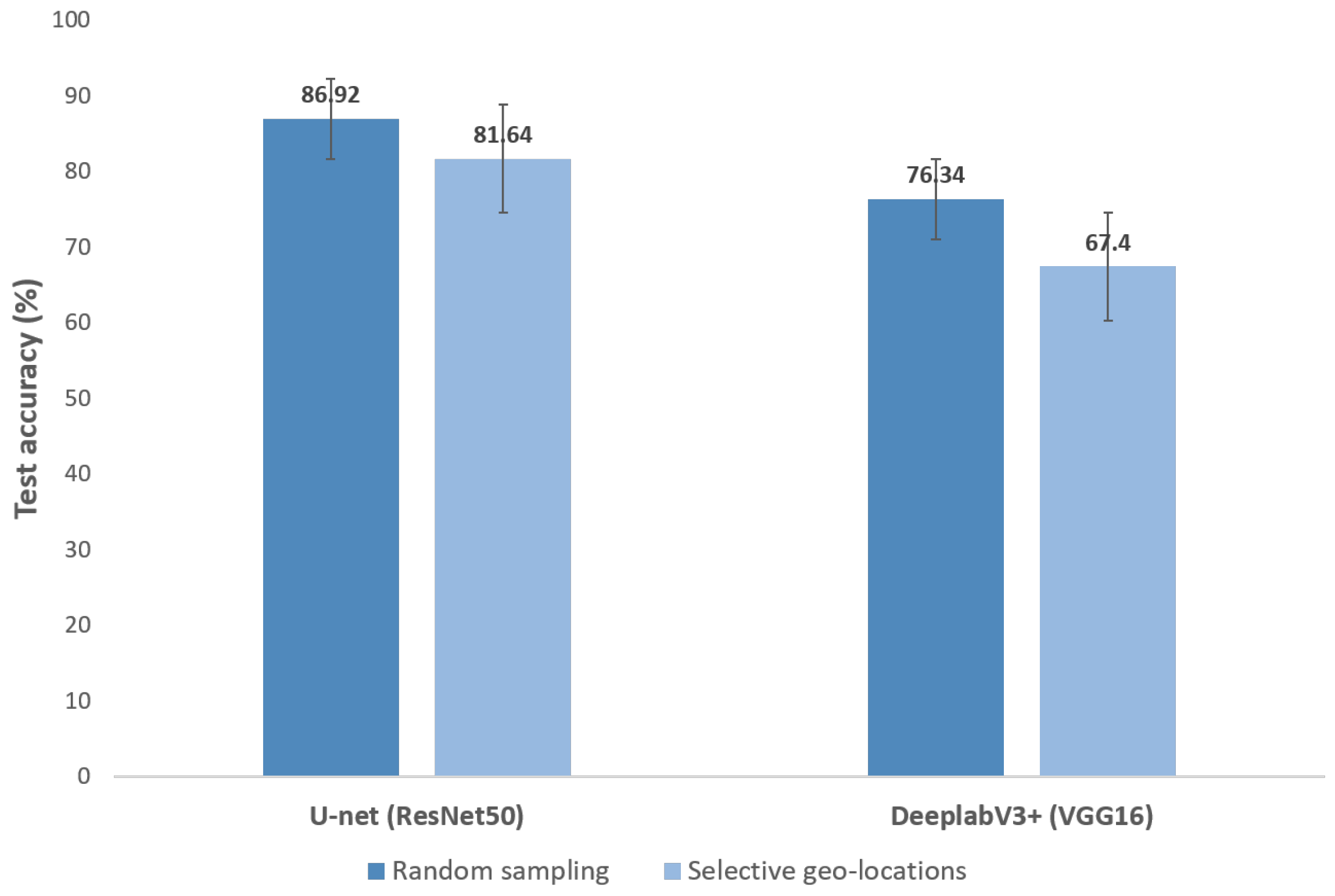
5.2. Model Sensitivity Analysis Using Randomly Sampled versus Specific Geo-Location Training Data

In this section, the two segmentation models are analysed regarding their sensitivity to the use of image patches from separate geo-locations for the train and test sets. The idea is to compare the effect of random sampling versus separate geo-locations on the model’s performance. Since the land cover characteristics vary from region to region in terms of types of materials and components, patterns of land use, and structures in both non-farm and farm area, e.g., types of crops, the nature of selected training, validation, and test image patches might vary when they are randomly selected over the whole ROI or when they are selected from different areas within the ROI, as shown in Figure 18. The former might lead to some sort of data leakage; therefore, a test for distinct geographical separation within the dataset was conducted. For this aim, the training image patches were exclusively sourced randomly from farms situated at distinct GPS coordinates compared to the testing set, ensuring a maximal geographical separation to prevent any spatial proximity between the two. Moreover, the validation image patches were curated deliberately from random farms positioned spatially between the training and testing areas. They were strategically chosen to maximize the overall geographical distance from both sets. This separation methodology guarantees enhanced robustness to data leakage and a certain degree of generalizability of the models, as it was tested on unseen data from locations that are significantly distant from those encountered during training. The image patches were meticulously selected from diverse locations across the Emilia-Romagna region, as shown in Figure 18, adhering to these stringent geographical criteria for a more comprehensive evaluation of the model’s accuracy. In Figure 19, the updated accuracy computations based on this curated testing dataset using RGB bands are presented. The best models from Table 2 and Table 3 were selected for this test. This refined separation strategy ensures that our model was evaluated for geographically distant data points, emphasizing its ability to generalize across diverse spatial settings within the region of interest.

5.3. Spectral Bands for Image Segmentation

To inspect the performance of multi-spectral band combinations we chose the U-Net architecture, which performed best for RGB imagery. All models for this set of experiments were trained from scratch without any pre-trained networks using the randomly sampled image patches from the ROI. Three sets of band combinations were tested: first, the regular RGB imagery; second, the red band was replaced by the NDVI index (as illustrated in (1), the NDVI was derived using the combination of red and NIR wavelengths); and, finally, third, we considered the band combination of NIR, SWIR, and blue. The results obtained are summarised in Table 4. It demonstrates the important role of additional information obtained by the multi-spectral band combination in improving the segmentation accuracy and MCC for farmlands. However, the MIoU shows some level of disagreement. Considering the importance of each of the three used metrics explained earlier at the end of Section 4.4.3, the second band combination, achieving the best performance in two of three metrics, can be considered, and to compensate for the MIoU results, some post-processing analyses can be carried out to fill the small non-farm pixels in the middle of the detected large farm regions to possibly improve the results in the segmented farm area. However, in this paper, only the original segmentation results are reported.

5.4. Synthetic Data Augmentation

5.4.1. Noise and Geometric Augmentation Results

We added noise, as well as geometric transformation, to the training data to expand them further. Salt-and-pepper noise, Gaussian noise, and random rotation were added. We continued to use the best model from Table 2 for all data augmentation experiments. The addition of noisy images and geometric transformation increased the performance of the best model marginally by 2.03%, to 90.97%, as compared to the test accuracy of 88.94% without any noise (Table 2).

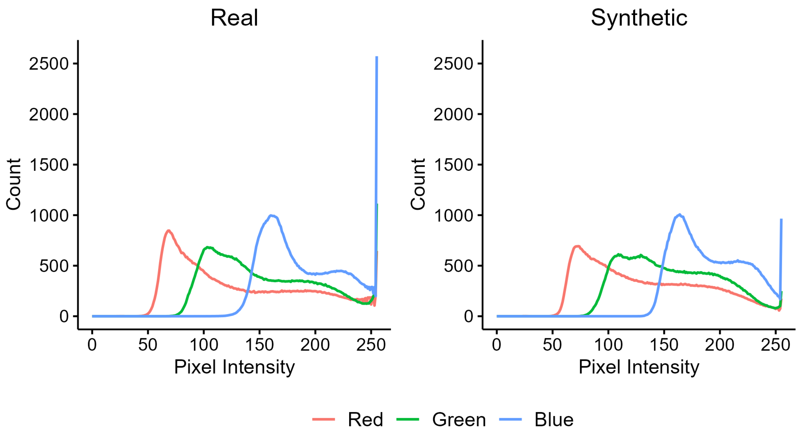
5.4.2. Testing the Quality of GAN-Generated Images

Two tests were performed to compare the quality of the generated images and the original training images. As shown in Figure 15, the generated image seems blurry. The variance and maximum of the Laplacian-applied images that were used for the evaluation of the edges are visualized in Figure 20. The Wilcoxon p value, as shown in Figure 20, is relatively small for the generated images, showing that the two populations are significantly different and supporting what was observed in blurry images. Furthermore, Figure 21 shows that the two image groups are very similar in terms of colour histogram distributions.

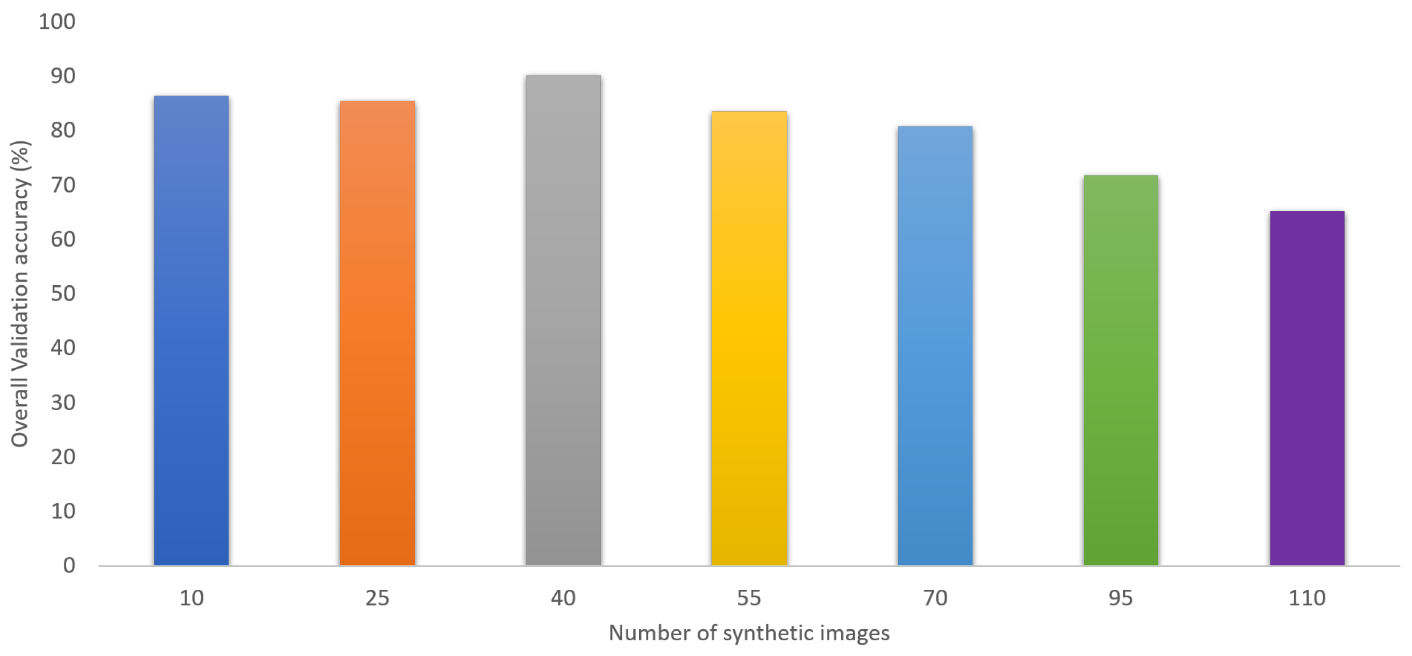
5.4.3. Segmentation Results Using Synthetic Imagery

To avoid major population deviation in the training sample, experiments were conducted with synthetic images in batches. Instead of adding all the generated images to the training dataset at once, small batches of synthesized images were introduced gradually, and the validation performance was considered to decide about adding any further augmented images. In earlier steps, 15 synthesized samples were added at each step, as shown in Figure 22. As can be seen, after adding a total of 40 artificial samples, the accuracy started to reduce. Therefore, it was concluded that the appropriate number of artificial samples to be added to the 175 original images in the train set of pure real samples is 40, corresponding to a percentage of ( 40 × 100 / 175 = 22.85 % ) of the real training samples. The results are summarised in Table 5.
CGAN-generated synthetic data further proved that accuracy can be improved if we expand the dataset; however, the quality of images and the number of generated images impact the model strongly.
In this paper, only RGB images were used to generate synthetic data, as they are easy and faster to train for GANs and have also produced decent accuracy in the past [76]; however, their use for generating other band combination images will be explored in future studies.

6. Discussion

This paper’s primary objective is to provide a comprehensive explanation of two distinct augmentation methods. The first method involves a diverse range of strategies, encompassing techniques such as image transformations and corruption. The second method centres on the generation of images using conditional generative adversarial networks (CGANs). The experimental results demonstrate the important role of the three identified factors in the semantic segmentation of farmlands. The results show that the segmentation model type and architecture, the type of used wavelengths, and the amount of training data can all influence the accuracy of the farm detection task. Below, we summarize the experimental findings with respect to model performance.

6.1. Effect of Deep Learning Architectures

In the case of supervised models, U-Net, though computationally expensive, performs the best with a limited dataset. Additionally, the inference time of both U-net and DeeplabV3+ were tested by taking an average of 10 runs on 10 test samples, and it was found that U-net (16.7 ms on average) consistently performs faster as compared to DeeplabV3+ (23.0 ms on average). In future research, we encourage the community to explore the potential of recent semantic segmentation models in addressing the challenge of semantic segmentation of farmlands. While this study is concentrated on U-Net and DeepLabv3+, we believe that the application of emerging models may offer valuable insights and advancements in this field.

6.2. Effect of IR Bands on Semantic Segmentation of Farmlands

Given the correlation of the IR band with the chemical characteristics of the land cover types, such as water stress in agricultural areas, the addition of the IR bands beside the visible bands improved the model performance.

6.3. Effect of Data Augmentation

Data augmentation showed a positive impact. It is crucial to not overwhelm the model with a large population of synthetically generated images and to maintain a good mix of real and synthetic images. In the case of the data used in this study, we found that adding 22% of synthetic images to the training set achieves the best results. In particular, our proposed strategy for systematic augmentation of CGAN-generated images was effective in improving the model’s accuracy. Overall, based on our findings, we conclude that leveraging the use of spectral bands and synthetic data can aid in accuracy improvement for limited amounts of labelled satellite imagery.

6.4. Effect of Training Data Sample Strategy

The analysis of segmentation models’ sensitivity when utilizing image patches from separate geo-locations for training and testing sheds light on the critical aspect of geographical diversity in dataset selection. We observe that the model is sensitive to different geo-locations, as demonstrated in Figure 19. By comparing the impact of random sampling versus distinct geo-locations on model performance, this study underscores the significance of considering regional variations in land cover characteristics. The deliberate separation of training and testing sets based on geographical coordinates ensures a rigorous evaluation process, mitigating the risk of data leakage and enhancing the models’ generalizability. This approach not only safeguards against spatial proximity bias but also facilitates a more comprehensive assessment of model accuracy across diverse landscapes within the ROI.
This paper’s findings can aid in developing robust models for identifying farmland from satellite images for applications requiring crop monitoring and yield prediction, which are significant, given the current urgent need to tackle world hunger. In this study, only single-season imagery was utilized. It would be worth exploring how these models perform for different seasons and times of the year using transfer learning strategies in the future. Finally, label scarcity can be averted by looking at unsupervised strategies for semantic segmentation; however, they are not as effective as the supervised suite of techniques. The lack of labelled training samples can lead to poor accuracy, especially for remote sensing images, as explicit knowledge about classes is vital to distinguish between different land cover types. The trained models might suffer from subjective error while labelling satellite images. On the other hand, unsupervised strategies struggle to capture contextual information from complex satellite imagery, given the diversity of land cover types; inter- and intra-class variation also impacts the segmentation maps adversely.

7. Conclusions

This paper thoroughly investigated and analyzed the pivotal factors influencing the efficacy of farm segmentation in mid-resolution satellite images. The study delved into various aspects, including the influence of distinct spectral bands, diverse model architectures, and the utilization of conditional generative adversarial networks (CGANs) for data augmentation, as well as the proposed systematic augmentation approach of gradually introducing synthetic images to the training population to test the performance improvement in conjunction with other image corruption and geometrically based augmentation techniques. Among the tested models, the combined employment of the U-Net model and ResNet exhibited the highest accuracy. Nonetheless, it is noteworthy that DeeplabV3+ models exhibit substantial potential for more accurate segmentation, considering the imagery’s resolution and complexity. The segmentation model’s accuracy was also studied in response to training and testing with image patches from distinct geographic locations, highlighting the impact of varied land cover characteristics. Additionally, perhaps the use of NIR bands could further improve the accuracy when trained on different GPS locations. Notably, this study highlights the imperative to develop new GAN architectures capable of generating both images and corresponding masks. Optimizing the augmentation strategy by determining the ideal number (about 22.85% of synthetic data) of augmented images to supplement the original training set helped to improve the semantic accuracy further when when a limited real labelled training samples were available. The promising outcomes from these experiments augur well for future advancements in both the precision and efficiency of farmland segmentation.
Moving forward, to enhance the quality of CGAN-generated images for future research, it is essential to focus on refining the architecture and training process of CGANs. Exploring techniques like progressive training, spectral normalization, and attention mechanisms can contribute to more stable and better-performing CGANs. Additionally, leveraging advanced loss functions such as perceptual loss or feature matching can guide CGANs to generate images with enhanced realism and finer details. Fine tuning the hyper-parameters, optimizing the generator–discriminator balance, and conducting rigorous evaluations of generated images against the ground truth can collectively lead to higher-quality image synthesis and pave the way for more accurate segmentation outcomes in subsequent studies. Moreover, the transfer of a pre-trained model to different seasons and/or different regions could lead to a shift in model accuracies due to various factors, such as the weather at the time of acquisition, illumination, angle of the satellite, etc. Different regions possess different characteristics, such as farming practices, crops grown, and seasons. These challenges underscore the importance of exploring potential solutions in future research endeavours.

Author Contributions

Conceptualization, S.N., S.S. and V.P.; methodology, S.N., S.S. and V.P.; software, S.N.; validation S.N., S.S. and V.P.; formal analysis, S.N.; investigation, S.N.; resources, S.N. and V.P.; data curation, S.N.; writing—original draft preparation, S.N.; writing—review and editing, S.N., S.S. and V.P.; visualization, S.N.; supervision, S.S. and V.P.; project administration, S.N.; funding acquisition, S.S. All authors have read and agreed to the published version of the manuscript.

Funding

This research was generously supported by the Global Challenges Research Fund (GCRF) call 2020–2021. We are grateful for the funding that enabled us to conduct this study.

Data Availability Statement

The data used in this work can be found at https://drive.google.com/drive/folders/1qGitO3Ys3D_PYZbY4W7w-RcEJ1D7SzEX?usp=drive_link (accessed on 1 December 2023).

Acknowledgments

The authors would like to thank Coventry University for the scholarship given to Shruti Nair. The authors would also like to express their sincere gratitude to Charley Hill-Butler for her kind support throughout.

Conflicts of Interest

The authors declare no conflicts of interest.

References

  1. Gap Report. Virginia Tech Cals Global. 28 September 2022. Available online: https://globalagriculturalproductivity.org/ (accessed on 10 May 2023).
  2. Decuyper, M.; Chávez, R.O.; Lohbeck, M.; Lastra, J.A.; Tsendbazar, N.; Hackländer, J.; Herold, M.; Vågen, T.G. Continuous Monitoring of Forest Change Dynamics With Satellite Time Series. Remote Sens. Environ. 2022, 269, 112829. [Google Scholar] [CrossRef]
  3. Hall, D.K.; Chang, A.T.; Siddalingaiah, H. Reflectances of Glaciers as Calculated Using Landsat-5 Thematic Mapper Data. Remote Sens. Environ. 1988, 25, 311–321. [Google Scholar] [CrossRef]
  4. Hong, X.; Chen, L.; Sun, S.; Sun, Z.; Chen, Y.; Mei, Q.; Chen, Z. Detection of Oil Spills in the Northern South China Sea Using Landsat-8 OLI. Remote Sens. 2022, 14, 3966. [Google Scholar] [CrossRef]
  5. Pandey, P.C.; Pandey, M. Highlighting the Role of Agriculture and Geospatial Technology in Food Security and Sustainable Development Goals. Sustain. Dev. 2023, 31, 3175–3195. [Google Scholar] [CrossRef]
  6. Landsat Satellite Missions|U.S. Geological Survey. Available online: https://www.usgs.gov/landsat-missions/landsat-known-issues (accessed on 10 May 2023).
  7. Sharifzadeh, S.; Tata, J.; Sharifzadeh, H.; Tan, B. Farm Area Segmentation in Satellite Images Using DeepLabv3+ Neural Networks. In Data Management Technologies and Applications; Communications in Computer and Information Science Book Series, CCIS; Springer: Cham, Switzerland, 2020; Volume 1255. [Google Scholar] [CrossRef]
  8. Chen, T.-H.K.; Qiu, C.; Schmitt, M.; Zhu, X.X.; Sabel, C.E.; Prishchepov, A.V. Mapping Horizontal and Vertical Urban Densification in Denmark with Landsat Time-Series from 1985 to 2018: A Semantic Segmentation Solution. Remote Sens. Environ. 2020, 251, 112096. [Google Scholar] [CrossRef]
  9. Zhong, L.; Hu, L.; Zhou, H. Deep Learning Based Multi-Temporal Crop Classification. Remote Sens. Environ. 2018, 221, 430–443. [Google Scholar] [CrossRef]
  10. Dou, P.; Shen, H.; Li, Z.; Guan, X. Time series remote sensing image classification framework using combination of deep learning and multiple classifiers system. Int. J. Appl. Earth Obs. Geoinform. 2021, 103, 102477. [Google Scholar] [CrossRef]
  11. Mirza, M.; Osindero, S. Conditional Generative Adversarial Nets. arXiv 2014, arXiv:1411.1784. [Google Scholar]
  12. Ronneberger, O.; Philipp, F.; Thomas, B. U-Net: Convolutional Networks for Biomedical Image Segmentation. In Proceedings of the Medical Image Computing and Computer-Assisted Intervention—MICCAI 2015, Munich, Germany, 5–9 October 2015. [Google Scholar] [CrossRef]
  13. Chen, L.; Zhu, Y.; Papandreou, G.; Schroff, F.; Adam, H. Encoder-Decoder with Atrous Separable Convolution for Semantic Image Segmentation. In Proceedings of the European Conference on Computer Vision (ECCV), Munich, Germany, 8–14 September 2018. [Google Scholar]
  14. Masek, J.G.; Wulder, M.A.; Markham, B.; McCorkel, J.; Crawford, C.J.; Storey, J.; Jenstrom, D.T. Landsat 9: Empowering Open Science and Applications through Continuity. Remote Sens. Environ. 2020, 248, 111968. [Google Scholar] [CrossRef]
  15. Lowe, D.G. Distinctive Image Features from Scale-Invariant Keypoints. Int. J. Comput. Vis. 2004, 60, 91–110. [Google Scholar] [CrossRef]
  16. Rosten, E.; Drummond, T. Fusing Points and Lines for High Performance Tracking. In Proceedings of the Tenth IEEE International Conference on Computer Vision (ICCV’05), Beijing, China, 17–21 October 2005. [Google Scholar]
  17. Dorj, U.O.; Lee, M.; Yun, S.S. An Yield Estimation in Citrus Orchards via Fruit Detection and Counting Using Image Processing. Comput. Electron. Agric. 2017, 140, 103–112. [Google Scholar] [CrossRef]
  18. Otsu, N. A Threshold Selection Method from Gray-Level Histograms. IEEE Trans. Syst. Man Cybern. 1979, 9, 62–66. [Google Scholar] [CrossRef]
  19. Ling, P.P.; Ruzhitsky, V.N. Machine vision techniques for measuring the canopy of tomato seedling. J. Agric. Eng. Res. 1996, 65, 85–95. [Google Scholar] [CrossRef]
  20. Achanta, R.; Shaji, A.; Smith, K.; Lucchi, A.; Fua, P.; Süsstrunk, S. SLIC Superpixels Compared to State-of-the-Art Superpixel Methods. IEEE Trans. Pattern Anal. Mach. Intell. 2012, 34, 2274–2282. [Google Scholar] [CrossRef]
  21. Chen, J.; Yang, C.; Xu, G.; Ning, L. Image Segmentation Method Using Fuzzy C Mean Clustering Based on Multi-Objective Optimization. J. Phys. Conf. Ser. 2018, 1004, 012035. [Google Scholar] [CrossRef]
  22. Yi, F.; Inkyu, M. Image Segmentation: A Survey of Graph-Cut Methods. In Proceedings of the 2012 International Conference on Systems and Informatics (ICSAI2012), Yantai, China, 19–20 May 2012; pp. 1936–1941. [Google Scholar] [CrossRef]
  23. Chen, M.; Artières, T.; Denoyer, L. Unsupervised Object Segmentation by Redrawing. arXiv 2019, arXiv:1905.13539. [Google Scholar]
  24. Xia, X.; Kulis, B. W-Net: A Deep Model for Fully Unsupervised Image Segmentation. arXiv 2017, arXiv:1711.08506. [Google Scholar]
  25. Teichmann, M.T.; Cipolla, R. Convolutional CRFs for Semantic Segmentation. arXiv 2018, arXiv:1805.04777. [Google Scholar]
  26. He, K.; Gkioxari, G.; Dollár, P.; Girshick, R. Mask R-CNN. arXiv 2018, arXiv:1703.06870. [Google Scholar]
  27. Chen, L.C.; Papandreou, G.; Kokkinos, I.; Murphy, K.; Yuille, A.L. DeepLab: Semantic Image Segmentation with Deep Convolutional Nets, Atrous Convolution, and Fully Connected CRFs. arXiv 2017, arXiv:1606.00915. [Google Scholar]
  28. Strudel, R.; Garcia, R.; Laptev, I.; Schmid, C. Segmenter: Transformer for Semantic Segmentation. arXiv 2021, arXiv:2105.05633. [Google Scholar]
  29. Giraud, R.; Ta, V.T.; Papadakis, N. Robust Superpixels Using Color And Contour Features Along Linear Path. Comput. Vis. Image Underst. 2018, 170, 1–13. [Google Scholar] [CrossRef]
  30. Wu, Z.; Gao, Y.; Li, L.; Xue, J.; Li, Y. Semantic segmentation of high-resolution remote sensing images using fully convolutional network with adaptive threshold. Connect. Sci. 2019, 31, 169–184. [Google Scholar] [CrossRef]
  31. Wu, J.; Chen, X.Y.; Zhang, H.; Xiong, L.D.; Lei, H.; Deng, S.H. Hyperparameter Optimization for Machine Learning Models Based on Bayesian Optimization. J. Electron. Sci. Technol. 2019, 17, 26–40. [Google Scholar] [CrossRef]
  32. Passos, D.; Mishra, P. A Tutorial on Automatic Hyperparameter Tuning of Deep Spectral Modelling for Regression and Classification Tasks. Chemom. Intell. Lab. Syst. 2022, 223, 104520. [Google Scholar] [CrossRef]
  33. Ma, L.; Liu, Y.; Zhang, X.; Ye, Y.; Yin, G.; Johnson, B.A. Deep Learning in Remote Sensing Applications: A Meta-Analysis and Review. ISPRS J. Photogramm. Remote Sens. 2019, 152, 166–177. [Google Scholar] [CrossRef]
  34. He, Y.; Wang, C.; Chen, F.; Jia, H.; Liang, D.; Yang, A. Feature Comparison and Optimization for 30-M Winter Wheat Mapping Based on Landsat-8 and Sentinel-2 Data Using Random Forest Algorithm. Remote Sens. 2019, 11, 535. [Google Scholar] [CrossRef]
  35. Wang, L.; Wang, J.; Liu, Z.; Zhu, J.; Qin, F. Evaluation of a Deep-Learning Model for Multispectral Remote Sensing of Land Use and Crop Classification. Crop J. 2022, 10, 1435–1451. [Google Scholar] [CrossRef]
  36. Peng, D.; Zhang, Y.; Guan, H. End-to-End Change Detection for High-Resolution Satellite Images Using Improved UNet++. Remote Sens. 2019, 11, 1382. [Google Scholar] [CrossRef]
  37. Kotaridis, I.; Lazaridou, M. Remote Sensing Image Segmentation Advances: A Meta-Analysis. ISPRS J. Photogramm. Remote Sens. 2021, 173, 309–322. [Google Scholar] [CrossRef]
  38. Alzubaidi, L.; Bai, J.; Al-Sabaawi, A.; Santamaría, J.; Albahri, A.S.; Al-dabbagh, B.S.N.; Fadhel, M.A.; Manoufali, M.; Zhang, J.; Al-Timemy, A.H.; et al. A Survey on Deep Learning Tools Dealing with Data Scarcity: Definitions, Challenges, Solutions, Tips, and Applications. J. Big Data 2023, 10, 46. [Google Scholar] [CrossRef]
  39. Hao, X.; Liu, L.; Yang, R.; Yin, L.; Zhang, L.; Li, X. A Review of Data Augmentation Methods of Remote Sensing Image Target Recognition. Remote Sens. 2023, 15, 827. [Google Scholar] [CrossRef]
  40. Safarov, F.; Temurbek, K.; Jamoljon, D.; Temur, O.; Chedjou, J.C.; Abdusalomov, A.B.; Cho, Y.-I. Improved Agricultural Field Segmentation in Satellite Imagery Using TL-ResUNet Architecture. Sensors 2022, 22, 9784. [Google Scholar] [CrossRef] [PubMed]
  41. Abady, L.; Horváth, J.; Tondi, B.; Delp, E.J.; Barni, M. Manipulation and Generation of Synthetic Satellite Images Using Deep Learning Models. J. Appl. Remote. Sens. 2022, 16, 046504. [Google Scholar] [CrossRef]
  42. Isola, P.; Zhu, J.-Y.; Zhou, T.; Efros, A.A. Image-to-Image Translation with Conditional Adversarial Networks. arXiv 2018, arXiv:1611.07004. [Google Scholar]
  43. Marín, J.; Escalera, S. SSSGAN: Satellite Style and Structure Generative Adversarial Networks. Remote Sens. 2021, 13, 3984. [Google Scholar] [CrossRef]
  44. Singh, P.; Komodakis, N. Cloud-Gan: Cloud Removal for Sentinel-2 Imagery Using a Cyclic Consistent Generative Adversarial Networks. In Proceedings of the IGARSS 2018—2018 IEEE International Geoscience and Remote Sensing Symposium, Valencia, Spain, 22–27 July 2018; pp. 1772–1775. [Google Scholar] [CrossRef]
  45. Weather Emilia-Romagna. 10 May 2023. Available online: https://www.meteoblue.com/en/weather/week/emilia-romagna_italy_3177401 (accessed on 10 May 2023).
  46. Regione Emilia-Romagna. Agriculture and Food. Available online: https://www.regione.emilia-romagna.it/en/agriculture-and-food (accessed on 10 May 2023).
  47. EarthExplorer. Available online: https://earthexplorer.usgs.gov/ (accessed on 10 May 2023).
  48. Young, N.E.; Anderson, R.S.; Chignell, S.M.; Vorster, A.G.; Lawrence, R.; Evangelista, P.H. A Survival Guide to Landsat Preprocessing. Ecology 2017, 98, 920–932. [Google Scholar] [CrossRef]
  49. Landsat 8 Data Users Handbook|U.S. Geological Survey. Available online: https://www.usgs.gov/landsat-missions/landsat-8-data-users-handbook/ (accessed on 10 May 2023).
  50. GISGeography. Landsat 8 Bands and Band Combinations. GIS Geography. 18 October 2019. Available online: https://gisgeography.com/landsat-8-bands-combinations/ (accessed on 10 May 2023).
  51. Chávez, P.S.J.; Mitchell, W.B. Computer Enhancement Techniques of Landsat MSS Digital Images for Land Use/Land Cover Assessments. 1977. Available online: http://pascal-francis.inist.fr/vibad/index.php?action=getRecordDetail&idt=PASCAL7930201432 (accessed on 10 May 2023).
  52. Armstrong, R.A. Remote Sensing of Submerged Vegetation Canopies for Biomass Estimation. Int. J. Remote Sens. 1993, 14, 621–627. [Google Scholar] [CrossRef]
  53. QGIS—A Free and Open Source Geographic Information System, Version 3.30.2. Available online: https://qgis.org/en/site/ (accessed on 10 May 2023).
  54. Shelhamer, E.; Long, J.; Darrell, T. Fully Convolutional Networks for Semantic Segmentation. arXiv 2015, arXiv:1411.4038. [Google Scholar]
  55. Hou, Y.; Liu, Z.; Zhang, T.; Li, Y. C-UNet: Complement UNet for Remote Sensing Road Extraction. Sensors 2021, 21, 2153. [Google Scholar] [CrossRef]
  56. Chen, Z.; Shi, B.E. Appearance-Based Gaze Estimation Using Dilated-Convolutions. arXiv 2019, arXiv:1903.07296. [Google Scholar]
  57. Chen, L.; Zhu, Y.; Papandreou, G.; Schroff, F.; Adam, H. Rethinking Atrous Convolution for Semantic Image Segmentation. arXiv 2017, arXiv:1706.05587. [Google Scholar]
  58. Rouse, J.W.; Haas, R.H.; Schell, J.A.; Deering, D.W.; Harlan, J.C. Monitoring the vernal advancements and retrogradation of natural vegetation. In NASA/GSFC; Final Report; NASA: Greenbelt, MD, USA, 1974; pp. 1–137. [Google Scholar]
  59. Agriculture Satellite Bands: Healthy Vegetation Band Overview. 6 June 2022. Available online: https://eos.com/make-an-analysis/agriculture-band/ (accessed on 10 May 2023).
  60. Negassi, M.; Wagner, D.; Reiterer, A. Smart(Sampling)Augment: Optimal and Efficient Data Augmentation for Semantic Segmentation. arXiv 2021, arXiv:2111.00487. [Google Scholar]
  61. Liu, S.; Zhang, J.; Chen, Y.; Liu, Y.; Qin, Z.; Wan, T. Pixel Level Data Augmentation for Semantic Image Segmentation Using Generative Adversarial Networks. In Proceedings of the ICASSP 2019—2019 IEEE International Conference on Acoustics, Speech and Signal Processing (ICASSP), Brighton, UK, 12–17 May 2019; pp. 1902–1906. [Google Scholar] [CrossRef]
  62. Ma, R.; Tao, P.; Tang, H. Optimizing data augmentation for semantic segmentation on small-scale dataset. In Proceedings of the 2nd International Conference on Control and Computer Vision, Jeju Island, Republic of Korea, 15–18 June 2019; pp. 77–81. [Google Scholar] [CrossRef]
  63. Wong, S.C.; Gatt, A.; Stamatescu, V.; McDonnell, M.D. Understanding Data Augmentation for Classification: When to Warp? In Proceedings of the 2016 International Conference on Digital Image Computing: Techniques and Applications (DICTA), Gold Coast, QLD, Australia, 30 November–2 December 2016; pp. 1–6. [Google Scholar] [CrossRef]
  64. Shorten, C.; Khoshgoftaar, T.M. A survey on image data augmentation for deep learning. J. Big Data 2019, 6, 60. [Google Scholar] [CrossRef]
  65. Van der Walt, S.; Schönberger, J.L.; Nunez-Iglesias, J.; Boulogne, F.; Warner, J.D.; Yager, N.; Gouillart, E.; Yu, T.; The Scikit-Image Contributors. scikit-image: Image processing in Python. PeerJ 2014, 2, e453. [Google Scholar] [CrossRef]
  66. Neff, T.; Payer, C.; Stern, D.; Urschler, M. Generative Adversarial Network Based Synthesis for Supervised Medical Image Segmentation. In Proceedings of the OAGM&ARW Joint Workshop 2017, Vienna, Austria, 10–12 May 2017. [Google Scholar] [CrossRef]
  67. Radford, A.; Metz, L.; Chintala, S. Unsupervised Representation Learning with Deep Convolutional Generative Adversarial Networks. arXiv 2016, arXiv:1511.06434. [Google Scholar]
  68. Kingma, D.P.; Ba, J. Adam: A Method For Stochastic Optimization. arXiv 2014, arXiv:1412.6980. [Google Scholar]
  69. Nair, V.; Hinton, G.E. Rectified linear units improve restricted boltzmann machines. In Proceedings of the 27th International Conference on Machine Learning (ICML-10), Haifa, Israel, 21–24 June 2010; pp. 807–814. [Google Scholar]
  70. Maas, A.L.; Awni, Y.H.; Andrew, Y.N. Rectifier nonlinearities improve neural network acoustic models. In Proceedings of the 30th International Conference on Machine Learning (ICML 2013), Atlanta, GA, USA, 16–21 June 2013; Volume 30, p. 3. [Google Scholar]
  71. Dubey, A.; Vanita, J. Comparative Study of Convolution Neural Network’s Relu and Leaky-Relu Activation Functions. arXiv 2019, arXiv:1511.06434. [Google Scholar]
  72. Goodfellow, I. NIPS 2016 Tutorial: Generative Adversarial Networks. arXiv 2016, arXiv:1701.00160. [Google Scholar]
  73. Sampath, V.; Maurtua, I.; Martín, J.J.A.; Gutierrez, A. A Survey on Generative Adversarial Networks for Imbalance Problems in Computer Vision Tasks. J. Big Data 2021, 8, 27. [Google Scholar] [CrossRef] [PubMed]
  74. Chicco, D.; Jurman, G. The Advantages of the Matthews Correlation Coefficient (MCC) over F1 Score and Accuracy in Binary Classification Evaluation. BMC Genom. 2020, 21, 6. [Google Scholar] [CrossRef] [PubMed]
  75. Cai, C.; Tan, J.; Zhang, P.; Ye, Y.; Zhang, J. Determining Strawberries’ Varying Maturity Levels by Utilizing Image Segmentation Methods of Improved DeepLabV3+. Agronomy 2022, 12, 1875. [Google Scholar] [CrossRef]
  76. Naushad, R.; Kaur, T.; Ghaderpour, E. Deep Transfer Learning for Land Use and Land Cover Classification: A Comparative Study. Sensors 2021, 21, 8083. [Google Scholar] [CrossRef] [PubMed]
Figure 1. Region of Emilia-Romagna, Italy.
Remotesensing 16 00823 g001
Figure 2. Landsat OLI 8 scene covering the region of Emilia-Romagna in two tiles/scenes (path 192–193 and row 029). Image obtained from USGS EarthExplorer [47].
Remotesensing 16 00823 g002
Figure 3. Dark object correction (DOC). (A) Originally dark raw Landsat 8 scene with values for different intensities at each pixel. (B) DOS- and colour-corrected Landsat tile.
Remotesensing 16 00823 g003
Figure 4. The overall analysis plan for the paper.
Remotesensing 16 00823 g004
Figure 5. Landsat image converted into 256 × 256 non-overlapping patches.
Remotesensing 16 00823 g005
Figure 6. Adapted U-Net architecture.
Remotesensing 16 00823 g006
Figure 7. Atrous convolution spatial pyramid pooling: different convolution rates explore the image to enhance the visual receptive fields [27].
Remotesensing 16 00823 g007
Figure 8. DeepLabV3+ architecture.
Remotesensing 16 00823 g008
Figure 9. Illustration of a 256 × 256 patch of an NDVI image randomly selected from Emilia-Romagna, covering around 1966.0 km2. The pixels in different levels of vegetation using the NDVI standard range are depicted in different colours. Translating the colours to numerical values, the no/low-vegetation areas are closer to −1, while the high-vegetation parts are close to +1.
Remotesensing 16 00823 g009
Figure 10. Illustration of the same 256 × 256 patch shown in Figure 9 in the format of an agriculture composite image shaped using SWIR, NIR, and blue bands. The patch is randomly selected from Emilia-Romagna, covering around 1966.0 km2. The healthy vegetation (vibrant green colour) appears different from the bare earth (magenta) and non-crop vegetation (pale green) [59].
Remotesensing 16 00823 g010
Figure 11. Illustration of a 256 × 256 patch of the image randomly selected from Emilia-Romagna, covering around 1966.0 km2. The original image patch, as well as the results of applying various types of noises to the same patch, is visualised, showing how the training images were augmented in the dataset.
Remotesensing 16 00823 g011
Figure 12. Geometric transformation.
Remotesensing 16 00823 g012
Figure 13. Modified CGAN with two-branched generators.
Remotesensing 16 00823 g013
Figure 14. (A) The generator is bifurcated into two channels: the top branch (visualized in orange), producing the generated image, and the bottom branch (visualized inside the grey box), producing the matching label/mask. (B) The discriminator architecture takes both the real and generated image–mask pairs as inputs to make predictions.
Remotesensing 16 00823 g014
Figure 15. (A) Generated images and (B) the corresponding generated masks. The white (1) label represents farms, and black (0) represents non-farms.
Remotesensing 16 00823 g015
Figure 16. Test accuracy comparison between U-net and Deeplabv3+ models.
Remotesensing 16 00823 g016
Figure 17. Resultant segmentation maps. In the mask array, the black (0) represents non-farms, and the white (1) represents farms in the masks. The model’s outputs for the segmentation of farms are visualized based on colours. Segmented farms are green, whereas red in the top row and blue in the bottom row are segmented non-farms.
Remotesensing 16 00823 g017
Figure 18. The RGB image patches for train/test/validation sets were chosen randomly from different geo-locations in the ROI to avoid unintentional data leakage.
Remotesensing 16 00823 g018
Figure 19. Comparison of testing accuracy for random data sampling and selected geo-location-based sampling.
Remotesensing 16 00823 g019
Figure 20. The high variance in plot A and the maximum of Laplacian measures shown in plot B were calculated for the real and CGAN-generated images. The comparison graphs show differences between the two groups of images, i.e., high for the original real image population, whereas the synthetic data showcase low values, indicating blurriness present in the GAN-generated imagery.
Remotesensing 16 00823 g020
Figure 21. The RGB colour histograms of the real population and the generated images. The overall colour scheme is identical.
Remotesensing 16 00823 g021
Figure 22. Illustration of the accuracy when synthetic data were added incrementally to the training set. The accuracy increases up to a certain point. However, it starts to degrade at some point (after adding more than 40 synthetic samples) due to the drift in the data population. The number of original real images was kept constant (175).
Remotesensing 16 00823 g022
Table 1. Description of Landsat 8 bands.
Band No.NameWavelength (μm)Resolution (m)Sensor
1Coastal aerosol0.43–0.4530OLI
2Blue0.45–0.5130OLI
3Green0.53–0.5930OLI
4Red0.63–0.6730OLI
5Near-Infrared (NIR)0.85–0.8830OLI
6Short-wave Infrared (SWIR) 11.57–1.6530OLI
7Short-wave Infrared (SWIR) 22.11–2.2930OLI
8Panchromatic0.50–0.6815OLI
9Cirrus1.36–1.3830OLI
10TIRS 12.11–2.2930 (100)TIRS
11TIRS 210.60–11.1930 (100)TIRS
Table 2. Results for U-Net model using RGB images; best model highlighted in bold.
Exp. No.Pre-Trained NetworksTrain AccuracyTest AccuracyMIoUMCC
1VGG1679.5776.7773.300.647
2ResNet5089.3486.9283.120.763
3ResNet10187.3283.4179.200.714
4MobileNetV274.2970.4768.380.608
Table 3. Results for DeeplabV3+ using RGB images; best model highlighted in bold.
Exp. No.Pre-Trained NetworksTrain AccuracyTest AccuracyMIoUMCC
5VGG1676.3474.2970.440.682
6ResNet5069.5967.3265.730.638
7ResNet10162.5160.9960.180.651
8MobileNetV273.9471.4568.240.619
Table 4. Comparison of segmentation results using different combinations of bands based on a newly trained U-Net model.
BandsTrain AccuracyTest AccuracyMIoUMCC
R-G-B87.8482.7779.300.689
NDVI-G-B92.9690.4972.900.700
NIR, SWIR1 and Blue88.2384.4268.760.652
Table 5. The train and test accuracy using UNET when synthetic data were introduced gradually to the 175 original RGB training images to avoid drastic data shifts.
RealSyntheticTotalTrain AccuracyTest AccuracyMIoUMCC
1751018580.9288.4577.250.640
1752520080.9277.2574.340.634
1754021591.1290.7188.300.716
1755523090.6586.5282.530.686
1757024589.2685.9580.720.649
1759527078.6474.7375.110.582
17511028571.2668.1872.960.532
Disclaimer/Publisher’s Note: The statements, opinions and data contained in all publications are solely those of the individual author(s) and contributor(s) and not of MDPI and/or the editor(s). MDPI and/or the editor(s) disclaim responsibility for any injury to people or property resulting from any ideas, methods, instructions or products referred to in the content.

