A Bidirectional Scoring Strategy-Based Transformation Matrix Estimation of Dynamic Factors in Environmental Sensing

Abstract

Simultaneous localization and mapping (SLAM) is the technological basis of environmental sensing, and it has been widely applied to autonomous navigation. In combination with deep learning methods, dynamic SLAM algorithms have emerged to provide a certain stability and accuracy in dynamic scenes. However, the robustness and accuracy of existing dynamic SLAM algorithms are relatively low in dynamic scenes, and their performance is affected by potential dynamic objects and fast-moving dynamic objects. To solve the positioning interference caused by these dynamic objects, this study proposes a geometric constraint algorithm that utilizes a bidirectional scoring strategy for the estimation of a transformation matrix. First, a geometric constraint function is defined according to the Euclidean distance between corresponding feature points and the average distance of the corresponding edges. This function serves as the basis for determining abnormal scores for feature points. By utilizing these abnormal score values, the system can identify and eliminate highly dynamic feature points. Then, a transformation matrix estimation based on the filtered feature points is adopted to remove more outliers, and a function for evaluating the similarity of key points in two images is optimized during this process. Experiments were performed based on the TUM dynamic target dataset and Bonn RGB-D dynamic dataset, and the results showed that the added dynamic detection method effectively improved the performance compared to state of the art in highly dynamic scenarios.

1. Introduction

With the rapid development of machine learning and computer science, autonomous navigation technology has been widely applied in technological and industrial fields, such as autonomous driving. Simultaneous localization and mapping (SLAM) [1] technology can realize autonomous navigation in unknown environments. Although the existing visual SLAM is still applied to realistic scenarios of some problems, previous studies often treated the external environment as a static assumption, thus ignoring the influence of dynamic objects in real environments on the accuracy of the SLAM algorithm, which eventually leads to inaccurate positioning information and serious deviations in the construction of an environmental map. To enhance the robustness and stability of SLAM in dynamic environments, scholars have eliminated the impact of dynamic objects on algorithms’ accuracy from two major perspectives. One method is the use of multi-view geometry [2] or other geometric constraint methods to detect outliers or dynamic regions with large residuals, while the other method is the introduction of deep learning into dynamic SLAM [3] and the use semantic information to segment some prior moving objects for elimination.

A dynamic detection scheme based on geometric constraints [4,5] has the advantages of high algorithmic efficiency and not requiring prior information on the target. Yu et al. proposed DS-SLAM [6] based on the ORB-SLAM2 [7] framework to distinguish static and dynamic features by using a geometric constraint method because the basic matrix calculated for the polar constraint was susceptible to external points, which then affected the system’s accuracy. Yao et al. divided dynamic and static areas by combining the distance error at the edge of an image [8] and used only the feature points extracted from the static area to estimate the camera pose, but the system’s stability was poor, and it was not sensitive to less dynamic moving targets. Zhang et al. employed the Random sample consensus algorithm (RANSAC) [9] along with feature-point-matching results to calculate an initial transformation matrix [10] between adjacent frames. Subsequently, this matrix was utilized for static weight assessment and static line feature extraction. Finally, the static line features were employed to accomplish the task of visual odometry. This method not only mitigated the impacts of dynamic objects on SLAM, but it also addressed the issue of tracking failure arising from the absence of point features in the environment. However, geometric constraint-based dynamic detection schemes exhibit an inherent limitation. The assumption of a predefined static area in the environment is a default setting, but it may not always hold true in real-world scenarios. For instance, in densely populated areas, dynamic targets often occupy larger spatial extents, thus deviating from the default setting of a static area.

On the other hand, in the application of visual SLAM in dynamic scenes, with the rise in neural networks, semantic segmentation has gradually been introduced into the semantic system of SLAM, and most network architectures include SegNet [11], Mask R-CNN [12], and the YOLO [13] series. Yu et al. proposed a DS-SLAM scheme that combined a visual SLAM algorithm with SegNet to delete semantic information in dynamic scenes, thus filtering out the dynamic parts of the scenes. This method improves the accuracy of pose estimation, but the types of objects identified by the semantic segmentation network in this scheme were limited, which also greatly limited its scope of application in practical scenarios. Bescos et al. proposed a dynamic and robust SLAM algorithm called DynaSLAM [14], which integrated a deep learning method and a multi-view geometry method to detect dynamic feature points in a scene. In RGB-D mode [15], the combination of a Mask R-CNN network and a multi-view geometric model was employed for moving object detection. However, a notable limitation of the system arose when applied to indoor environments with complex dynamic factors. Specifically, the Mask R-CNN network proved to be less effective in accurately segmenting less dynamic targets.

Hence, we propose a semantic SLAM algorithm based on geometric constraints to address the limitations identified in the aforementioned geometric and semantic approaches. Firstly, we designed feature matching constraints aimed at eliminating numerous mismatches between feature point pairs. By leveraging the relationship between the closest and second-closest Hamming distances of the feature point pairs, a matching quality score was computed and utilized to impose constraints on the feature point matching. Secondly, a bidirectional scoring strategy was introduced to eliminate the most dynamic feature points. A geometric constraint function was defined based on the Euclidean distance between corresponding feature points and the average distance of the corresponding edges. Abnormal scores were determined by using this constraint function, enabling the identification and elimination of highly dynamic feature points. Finally, the estimation of a transformation matrix was applied to the filtered feature points for the further removal of outliers. In this step, intrinsic constraints between samples guided selective sampling. Dynamic feature points were initially filtered out through coarse filtering. Subsequently, an evaluation function for the similarity of key points in two images was improved and optimized to achieve the accurate matching of key point pairs. This three-step process collectively enhanced the feature matching accuracy and robustness in handling dynamic scenes.

2. Overall Structure

This study proposes a system that is built upon the semantic SLAM framework, as shown in Figure 1. Two threads proceed in parallel: The first uses a Mask R-CNN network segmentation model to segment an indoor scene, while in the second, the improved system adds a dynamic feature point filtering module to filter out the feature points (marked in a red rectangular box).

In the first thread, we initially employ Mask R-CNN to detect dynamic objects in each input frame, performing pixel-wise segmentation on dynamic objects with prior information (e.g., humans). However, the semantic segmentation model exposes some issues in dynamic detection: movable dynamic objects such as chairs cannot be semantically segmented due to the lack of prior information in the neural network model, and the legs or hands of humans cannot be segmented due to model accuracy limitations. These unfiltered dynamic feature points may introduce additional noise and instability, affecting the robustness and accuracy of navigation. Therefore, based on the segmentation results from Mask R-CNN, we propose a geometric dynamic feature filtering algorithm to further filter out objects without prior information and human limbs that are not segmented. In the second thread, ORB feature points are extracted from the current image frame, and feature point pair matching is accelerated by using the Bag-of-Words model [16] based on the BRIEF descriptor between the matching point pairs. Initially, we establish a bidirectional scoring strategy for filtering out highly dynamic feature points. This strategy utilizes the geometric discrepancy of corresponding edges between adjacent frames, assigning abnormal scores to the two feature points on these edges. Subsequently, we utilize a transformation matrix estimation based on the filtered feature points to remove additional outliers. During this process, a function for evaluating the similarity between key points in two images is optimized. This module effectively segments both dynamic objects with no prior information and potential dynamic objects identified by the CNN. Ultimately, the filtered static feature points are used for pose estimation.

2.1. Bidirectional Scoring Strategy for the Filtering of Dynamic Feature Points

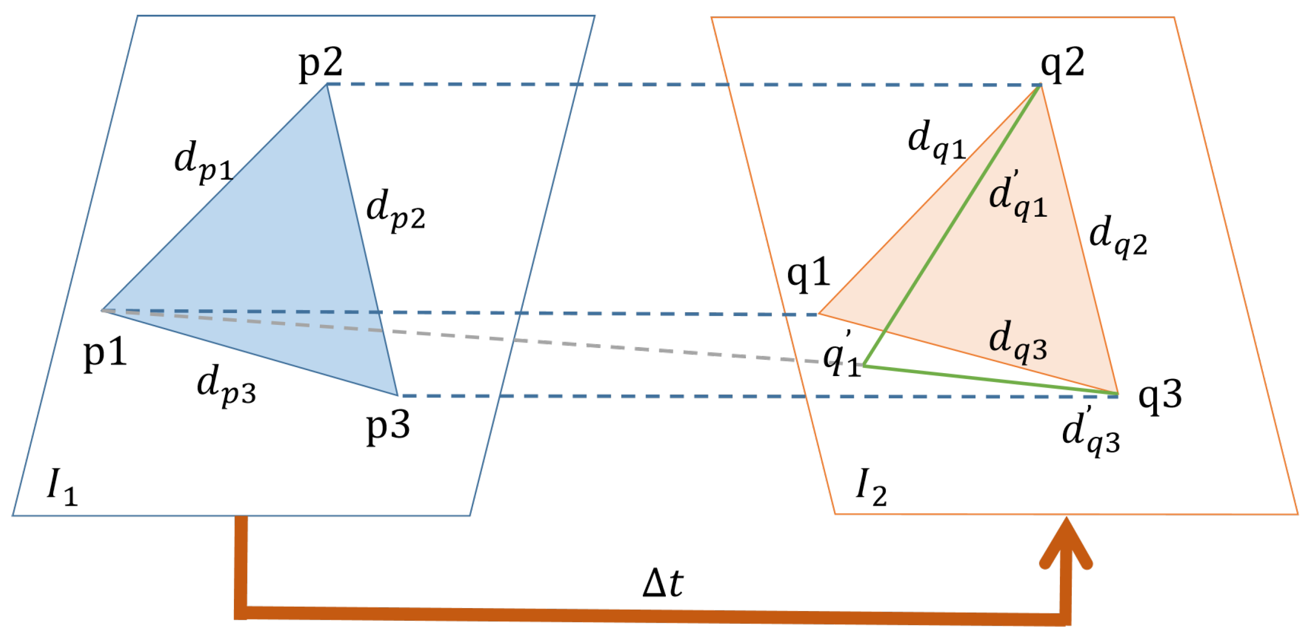
Figure 2 shows a conceptual diagram of bidirectional scoring strategy for the filtering of dynamic feature points. The part inside the blue rectangular box is the accuracy constraint for matching points. In the stage of image feature point matching, we identified matching point pairs when the maximum Hamming distance was significantly larger than the second-closest Hamming distance; then, they were classified as reliable matches. The portion inside the green rectangular box represents our bidirectional scoring strategy. After passing through the accuracy constraint for image feature points, the feature point pairs had a relatively accurate matching relationship, but dynamic feature points were also retained. To further filter out the dynamic feature points in a scene, this study introduced a geometric constraint model of the image feature points, as shown in Figure 3. The query image $I_1$ and the target image $I_2$ are two adjacent frames, and the sampling time interval between them is very short; therefore, the camera projection distortion caused by the camera’s pose transformation is very small. The triangle vertices in the figure represent the extracted ORB feature points, with three pairs forming two triangles $▵p_1{p}_2{p}_3$ and $▵q_1{q}_2{q}_3$ on $I_1$ and $I_2$; the vertices $p_1$, $p_2$, and $p_3$ are the three feature points on $I_1$, and they match the three feature points $q_1$, $q_2$, and $q_3$ on $I_2$, respectively. Furthermore, each side, d, of the triangle is the Euclidean distance [17] between the feature points.

In the context of dynamic SLAM, the decision to employ an exponential function for characterizing geometric constraint scoring functions stems from the distinctive properties inherent in the exponential function. The exponential function serves the crucial purpose of mapping the disparities in geometric constraint scores onto a non-negative range. Through exponentiation, this design ensures that scores corresponding to minor differences in geometric constraints converge towards 1, while scores associated with more significant differences experience rapid growth. This mapping relationship proves invaluable for accentuating subtle differences in geometric constraint scores, thus enhancing the sensitivity and facilitating the differentiation between static and dynamic feature points.

Apart from the exponential function, other functions can also be used to characterize geometric constraint scoring functions, but they all have certain limitations. For instance, linear functions may lack sensitivity in representing minor geometric constraint differences due to their linear variations. Logarithmic functions may prove to be overly responsive, particularly in the presence of minor geometric differences. Sigmoid functions may exhibit saturation under certain circumstances, resulting in inadequate sensitivity in extreme cases.

The selection of the exponential function is guided by its unique ability to distinctly express score differences, providing a nuanced representation of changes in geometric relationships. In the dynamic SLAM domain, where sensitivity to subtle geometric differences is pivotal, the exponential function emerges as a commonly employed and effective choice.

When there is no dynamic target in the image frame, the difference between the corresponding edges of the triangle should be in a small interval; to better describe this relationship, a geometric constraint score function $q_g(i,j)$ is defined as follows:

$$q_g(i,j)=exp\left(⌊\frac{d\left(p_i,p_j\right)-d\left(q_i,q_j\right)}{A(i,j)}⌋\right)$$

(1)

where $d(m,n)$ represents the Euclidean distance between the feature points m and n, and $A(i,j)$ represents the average distance between the two corresponding edges, which can be expressed as follows:

$$A(i,j)=\frac{d\left(p_i,p_j\right)+d\left(q_i,q_j\right)}{2}$$

(2)

If a dynamic target appears in the scene, assuming that the point $q_1$ is on the dynamic target, then $q_1$ on the target image moves to the new position $q_1^{\prime }$, thus constituting the new triangle $▵q_1^{\prime }{q}_2{q}_3$, and the Euclidean distances between the two vertices of the triangle are $d_{q1}^{\prime }$, $d_{q2}^{\prime }$, and $d_{q3}^{\prime }$. Because the position of the $q_1$ point changes, the value of the geometric constraint score function calculated with the geometric constraint score function $q_g(i,j)$ will be abnormally large, so we need to eliminate the dynamic feature points, but the geometric constraint score involves two pairs of feature points, and real dynamic feature points are usually difficult to determine. In light of this, this study proposes a bidirectional feature point scoring strategy for identifying the real dynamic feature points in a scene. The main idea is to define the abnormal score of a characteristic point. When an exception appears on a side, one point each will be added to the abnormal scores of the two characteristic points on that side. In this way, there will be a significant gap between the real dynamic features and the static feature points. Moreover, it is easy to know that the anomalous score of a feature point represents how many feature points are needed to judge a point as an abnormal dynamic point. The geometric expression of an anomalous score of feature points is

$$q_{\mathit{ab}}\left(i\right)=\sum _{j=0}^{M}s(i,j)$$

(3)

where $q_{ab}\left(i\right)$ is the anomalous score of the ith characteristic point, and $s(i,j)$ represents the increment in the abnormal score, as follows:

$$s(i,j)=\left\{\begin{array}{c}1,q_g(i,j)>\beta \times AS\hfill \\ 0,\mathrm{else}\hfill \end{array}\right.$$

(4)

where $\beta$ is the mean score scale factor of the geometric constraint, which controls its strictness. Regarding the range of the average score scale factor $\beta$, it is typically set between 0.1 and 0.5, striking a balance between sensitivity to dynamic changes and stability in static scenes. During the tuning process, the final value for $\beta$ was determined to be 0.2. This specific choice ensured that the geometric constraint scoring exhibited a robust response to dynamic targets in dynamic scenes while maintaining relative stability in static scenes. $AS$ denotes the mean geometric score between the pairs of points in an image:

$$AS=\frac{1}{n}\sum _{i,j=1}^n{w}_s^{i,j}{q}_g(i,j)$$

(5)

where n is the number of matching image feature points, $q_g(i,j)$ denotes the geometric scores of two matching feature points i and j, and $w_s$ is the geometric error weight factor between the matching feature points, which reduces the influence of a large geometric constraint on the calculation of the mean score.

As shown in Figure 4a, we extracted 500 ORB feature points from a dynamic image. The distribution of their abnormal scores is shown in Figure 4b, where the x-axis represents the total number of feature points, the y-axis describes the anomalous score value for a specific feature point, and the red line represents the segmentation threshold, which means that when an abnormal score of a feature point is greater than the threshold, it is judged as a dynamic feature point. We set the adaptive dynamic segmentation threshold [18] to $\gamma M$, where M is the total number of extracted feature points, and $\gamma$ is set to 80% in Figure 4.

2.2. Transformation Matrix Estimation

The pose transformation relationship between image frames can be represented by a fundamental matrix. In this study, we propose an algorithm that incorporates intrinsic constraints between samples to guide selective sampling with the aim of obtaining an improved fundamental matrix. Firstly, dynamic feature points in a scene were filtered out through coarse filtering. Then, the function for the evaluation of the similarity of key points in two images was improved, and it was optimized to achieve accurate matching of the key point pairs. Figure 5 illustrates a conceptual diagram of the transformation matrix estimation.

If there exists a correct pair of matching points $(P_i,Q_i)$ and $(P_j,Q_j)$, $d(P_i,P_j)$ is the distance from $P_i$ to $P_j$, $d(Q_i,Q_j)$ is the distance from $Q_i$ to $Q_j$, and the two distances are similar. We found the relationship between $P_i$ and all associated points $P_j$ in the first image and the relationship between $Q_i$ and all associated points $Q_j$, then used their similarity to evaluate the correspondence of the two points; thus, the following evaluation functions are proposed:

$$\omega \left(i\right)=\sum \frac{r(i,j)}{1+D(i,j)}$$

(6)

where the average distance between $P_i$ and $Q_i$ with each pair of associated points is

$$D(i,j)=\left[d\left(P_i,P_j\right)+d\left(Q_i,Q_j\right)\right]/2$$

(7)

$$r(i,j)=exp\left(-u_{ij}\right)$$

(8)

$$u_{ij}=\left|d\left(P_i,P_j\right)-d\left(Q_i,Q_j\right)\right|/D(i,j)$$

(9)

where $u_{ij}$ is the difference in similarity between $P_i$ and $Q_i$ for each pair of associated points.

The following is the procedure for estimating the transformation matrix:

• All values of $w_i$ are calculated.
• The mean w of all $w_i$ is found.
• $w_i$ is judged: If $w_i>0.8w$, $P_i$ and $Q_i$ are correct similarities, and they are retained; otherwise, they are deleted.
• The filtered point pair with the correct similarity is taken as the initial iterative feature point pair for the RANSAC algorithm.
• The point pair with the correct similarity is used as a candidate matching feature set. Four groups are randomly selected to establish equations and calculate the unknowns in the transformation matrix M for the estimation of the transformation matrix.
• The distances between other feature points and the candidate matching points are calculated by using the transformation model, and the threshold r is set. When the distance is less than this threshold, the feature point is determined to be an inlier; otherwise, it is an outlier.
• The inliers are used to re-estimate the transformation matrix for N iterations.

3. Experiments and Analysis

3.1. Experimental Environment and Datasets

To evaluate the efficacy of the proposed algorithm in our SLAM system, we performed comprehensive evaluations by using the TUM RGB-D dataset and the dynamic Bonn RGB-D dataset. The upgraded version of our system underwent rigorous testing and comparative analysis against benchmark systems such as ORB-SLAM3 [19] and DynaSLAM to gauge its performance improvements. All experiments were conducted on a high-performance computing setup comprising an Intel(R) Core(TM) i9-10900X CPU, RTX3070 GPU, and 64 GB of memory and operating in the Ubuntu 18.04 environment. This robust setup ensured reliable and consistent experimental conditions, allowing for a thorough assessment of our algorithm’s capabilities and advancements in real-time SLAM applications.

The TUM RGB-D dataset is a widely used computer vision dataset that is mainly used for visual SLAM research, and it includes a series of RGB and depth images of indoor scenes, as well as corresponding camera motion trajectories. We used the Dynamic Objects category in the TUM RGB-D dataset, which contains dynamic objects recorded with an Asus Xtion sensor. The dataset that we tested had a total of eight sequences: the sitting_static, sitting_xyz, sitting_halfsphere, sitting_rpy, walking_static, walking_xyz, walking_halfsphere, and walking_rpy image sequences. These sequences were of two types, as shown in Figure 6: sitting sequences and walking sequences. In the sitting sequences, two people sat at a table, chatted, spoke, and made some gestures. In the walking sequences, two people stood up, walked through an office, and finally sat back down in their original positions. Each type also included four types of sensor movements: static—the sensor was manually fixed; xyz—the sensor moved in three directions (xyz); rpy—the sensor rotated along the main axis; halfsphere—the sensor moved on a hemisphere with a diameter of approximately 1 m.

The dynamic Bonn RGB-D dataset—provided by the University of Bonn (BONN)—is an open-source indoor RGB-D dataset that was captured using ASUS Xtion PRO LIVE. The dataset offers real-motion trajectories obtained through dynamic calibration, and it follows the same format and evaluation methodology as those of the TUM dataset. It emulates various complex scenarios in real life, demonstrating strong representativeness for authentic environments. The dataset includes multiple types of complex real-world motions, such as crowd movement, individual person tracking, simultaneous parallel motions, balloon motion, and object transport motion, among others. We selected three representative sequences for testing, as illustrated in Figure 7: rgbd_bonn_balloon, rgbd_bonn_crowd3, and rgbd_bonn_person_tracking2.

To evaluate our improved system in comparison with other SLAM methodologies, we utilized the absolute pose error (APE) and relative pose error (RPE) to measure the accuracy of the camera trajectories. These served as foundational metrics and were complemented by an array of statistical analyses involving the root-mean-squared error (RMSE), sum of squared errors (SSEs), mean, and median. The deployment of these diverse metrics enabled a comprehensive and in-depth evaluation of our system’s tracking accuracy and robustness. By comparing these metrics with those of other SLAM methods, we discerned nuanced performance variations and drew more insightful conclusions regarding the advantages and limitations of our enhanced system.

3.2. Feature Point Matching Based on the Bidirectional Scoring Strategy

To comprehensively validate the efficacy of our geometric constraint algorithm for image feature point matching, we selected the freiburg3_walking_static sequence from our dataset as an experimental input. This sequence was deliberately chosen to assess the algorithm’s performance under dynamic scenarios where objects rapidly transition. Specifically, our investigation focused on examining the filtering impacts of two crucial components of the algorithm: the matching distance accuracy constraint module and the bidirectional scoring strategy. By scrutinizing their effects on feature points in scenarios characterized by swift dynamic changes, our study aimed to provide robust evidence and insights into the algorithm’s ability to handle such dynamic scenes. Through this analysis, we sought to highlight the algorithm’s strengths and limitations under challenging dynamic conditions, enhancing the understanding of its practical utility and performance in real-world scenarios.

Figure 8 shows the filtering results of the algorithm for ORB feature matching when using the test data. In the experimental process, two images of a person quickly standing up in the same scene were selected, as shown in Figure 8a. The experiments were divided into two groups; the first group is shown in Figure 8b, and the traditional ORB feature matching method was used to perform an image registration experiment on two images. For the second group, as shown in Figure 8c, the distance accuracy constraint on feature point pairs was utilized to filter out the mismatching of the first group of matched results. From the filtering results, it can be seen that our algorithm was able to effectively reduce the misjudgment of similar feature points, thereby obtaining more accurate matching point pairs.

The matching accuracy constraint module significantly reduced the number of ORB feature mismatches in the scene. However, feature points within the dynamic target area could still be extracted. To address this, we further employed a bidirectional scoring strategy to filter out feature points with abnormal scores located in the dynamic area. Figure 9 visually demonstrates the effectiveness of the bidirectional scoring strategy in eliminating feature matching point pairs across most regions of the human body, in addition to the matching accuracy constraints that were already applied.

3.3. Feature Point Filtering Based on the Estimation of a Transformation Matrix

Although the aforementioned geometric constraints help eliminate feature points on dynamic objects, some feature points can still be extracted from certain dynamic regions (human hands, feet, etc.). Therefore, we used a novel method of transformation matrix estimation to filter out more outliers. In this experimental evaluation, the freiburg3_sitting_xyz (fr_s_xyz) and freiburg3_walking_xyz (fr_w_xyz) sequences were tested, and the results were compared with those of ORB-SLAM3 and DynaSLAM. The purpose of this comparison was to validate the effectiveness of the transformation matrix estimation in suppressing dynamic feature points.

For the adaptive threshold method that targeted feature points with anomalous scores (described in Section 2.1), we conducted an experiment comparing the precision (based on the fr_w_xyz sequence) to determine the optimal threshold value ($\gamma$). APE metrics—specifically, the mean and RMSE—were selected as indicators of the trajectory accuracy. The mean provided an intuitive understanding of the overall performance, while RMSE emphasized higher sensitivity to significant errors, offering a comprehensive evaluation of the SLAM system’s trajectory estimation accuracy in the combined experiments. As shown in

Table 1. Trajectory accuracy comparison with varying $\gamma$ in an adaptive threshold experiment.

$\mathit{\gamma }$	Mean	RMSE
60%	0.0652	0.0693
70%	0.0447	0.0481
80%	0.0281	0.0235
90%	0.0637	0.0693

, we varied $\gamma$ from 60% to 90% and conducted the trajectory accuracy comparison experiments at 10% intervals. It was evident that when $\gamma$ was set to 80%, both the mean and RMSE reached their minimum values, indicating that the highest accuracy in the SLAM trajectory estimation was at this threshold.

Figure 10a shows the feature point extraction effect of ORB-SLAM3 in dynamic scenes, Figure 10b shows the feature point filtering effect of DynaSLAM in dynamic regions, and Figure 10c shows the feature point filtering results of the transformation matrix estimation in dynamic regions; green dots represent the positions of ORB feature points. In Figure 10a, it can be seen that ORB-SLAM3 did not perform any processing on dynamic objects, and the feature points of the dynamic area were preserved.

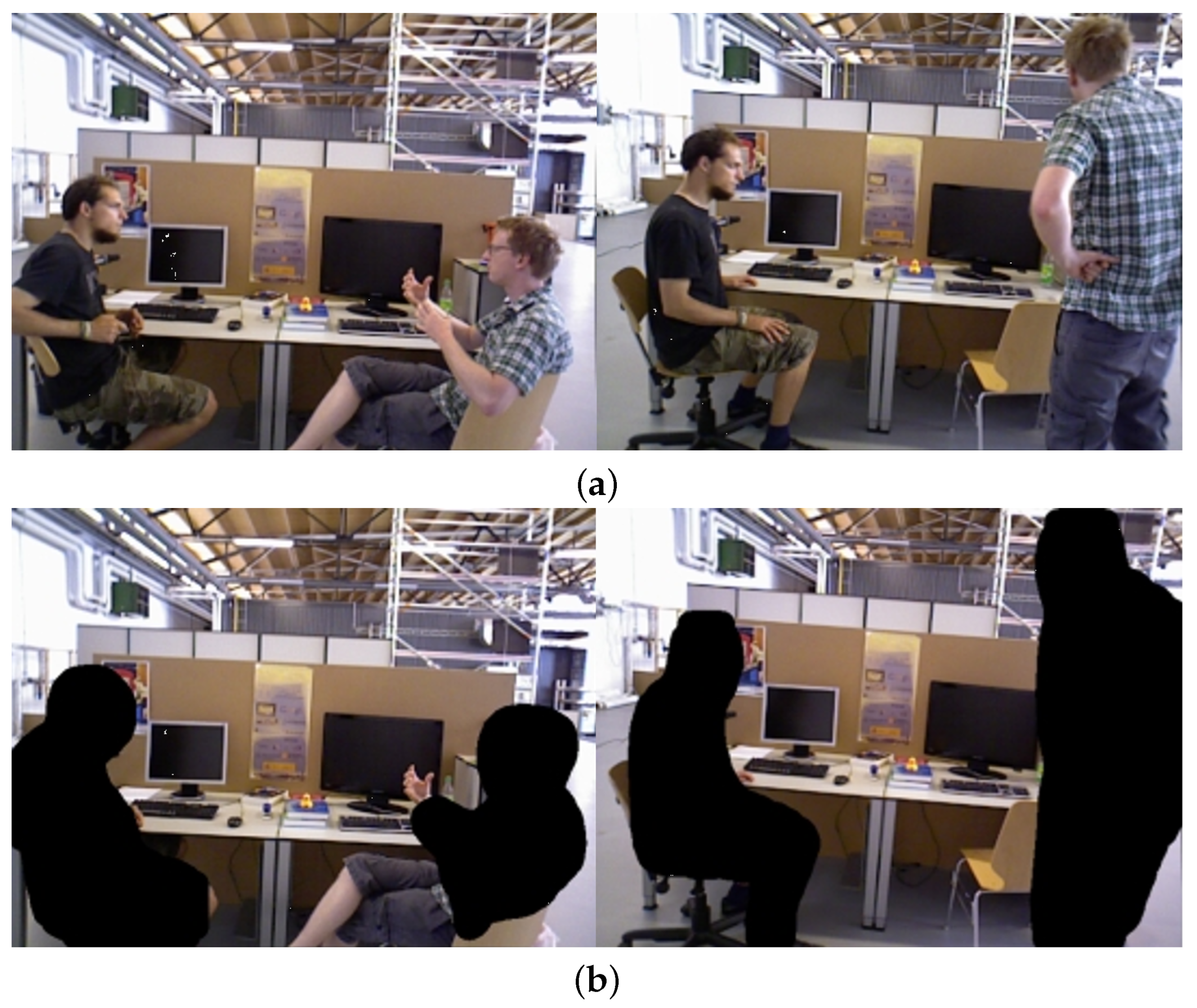
In Figure 10b, it can be seen that DynaSLAM’s scene segmentation model using Mask R-CNN detected and removed feature points that fell on dynamic objects while retaining other feature points that fell on static objects. However, one can see in the left image that the leg feature points of the person sitting on the right were not filtered out. In addition, one can see in the image on the right that the feature points on potential dynamic objects, such as chairs, were not completely filtered out. As shown in Figure 11, Mask R-CNN did not accurately segment the legs and hands of the person in the sitting sequence because the semantic segmentation model had poor segmentation accuracy for less dynamic objects (the right person’s leg hardly moved). Mask R-CNN did not fully segment the chairs in the walking sequence on the right because it lacked prior information about potential dynamic objects, such as chairs, when training the network model.

In Figure 10c, it can be clearly seen that the majority of the feature points on the legs of the person in the left image and the feature points on the chairs in the right image were filtered out, with only a few feature points remaining in the contour of the dynamic target. This indicated that the transformation matrix estimation was able to effectively compensate for the shortcomings of semantic segmentation with Mask R-CNN, thereby improving the suppression of dynamic feature points.

In our study, we devised an experiment to quantify the average number of feature point matches and the trajectory accuracy (RMSE) across eight dynamic sequences from the TUM dataset while comparing three SLAM systems. The primary focus was on highlighting the enhancements offered by our proposed approach concerning the removal of abnormal feature points and the accuracy of trajectory reconstruction in comparison with DynaSLAM.

Table 2. Comparison of feature point matches and trajectory accuracy in dynamic sequences.

Comparative Experiments	ORB-SLAM3		DynaSLAM		Proposed		Improvement on DynaSLAM
Feature Matching and APE	Matches	RMSE	Matches	RMSE	Matches	RMSE	RMSE
freiburg3_sitting_halfsphere	462	0.0430	198	0.0245	146	0.0240	2.91%
freiburg3_sitting_rpy	396	0.9839	176	0.9460	122	0.2591	72.60%
freiburg3_sitting_static	411	0.5759	171	0.2147	133	0.1270	40.87%
freiburg3_sitting_xyz	389	0.0270	185	0.0210	145	0.0175	16.77%
freiburg3_walking_halfsphere	367	0.7125	163	0.0230	159	0.0225	2.19%
freiburg3_walking_rpy	335	0.7551	153	0.1319	110	0.1125	14.69%
freiburg3_walking_static	459	2.7401	203	0.1710	172	0.1331	22.63%
freiburg3_walking_xyz	312	1.7032	189	0.0255	132	0.0235	7.68%

illustrates that, in contrast to ORB-SLAM3, both DynaSLAM and the proposed method excelled in eliminating a significant proportion of the dynamic feature points within the scenes. Particularly, in comparison with DynaSLAM, which incorporated dynamic detection capabilities, the proposed method demonstrated superior efficacy in eliminating more matching feature points associated with potential dynamic targets, leading to a noticeable improvement in the RMSE. In the experiments based on the freiburg3_walking_halfsphere (fr_w_halfsphere) sequence, due to the rapid rotation of the camera, the dynamic targets in the scene are mostly the upper bodies of two individuals, and the neural network model of DynaSLAM was capable of semantically segmenting these targets. Therefore, the proposed method extracted nearly the same number of feature points as that of DynaSLAM in the scene, and the improvement in trajectory accuracy was also limited. In the experiments based on the fr_w_xyz sequence, the proposed method removed numerous matching feature points, including some from static scenes, such as computer-generated features. This was because the rapid motion of dynamic objects in this sequence, along with the fast shaking of the camera, may have led to the failure to extract static feature points, and motion blur, defocused effects, disparity, and feature occlusion were the main contributing factors. Additionally, the camera underwent parallel motion, causing the feature points in the image frames to move on a nearly flat plane with minimal depth variations. This situation may have introduced errors into the algorithm’s motion estimation, leading to the removal of some static feature points. However, our trajectory accuracy still showed some improvements. Therefore, the observed phenomenon of removing static feature points in Figure 10c is common in dynamic environments, but it does not compromise the effectiveness of our method in enhancing the performance of SLAM while maintaining the representation integrity of static environments.

3.4. Three-Dimensional Pose Tracking Accuracy

Figure 12 shows the APE of ORB-SLAM3, DynaSLAM, and the proposed system on the highly dynamic sequence fr3_w_static. The gray line represents the ground truth of the camera, while the colored line represents the camera trajectory estimated with the SLAM algorithm. In highly dynamic environments, there is a significant difference between the motion trajectory estimated by the ORB-SLAM3 system and the ground truth, and even erroneous trajectories may occur in certain areas. On the contrary, DynaSLAM and the proposed system had a large overlap in their estimations of the motion trajectories and real trajectories, and the proposed system was closer to the real trajectories. This indicated that the method in this article was more capable of handling highly dynamic scenarios.

Figure 13 shows how the APE on the highly dynamic sequence fr3_w_static changed over time, and colored curves are used to represent errors, such as the RMSE, mean, and median. It can be clearly seen that our method had higher accuracy at almost all times. Our method also had better robustness than that of traditional methods when facing different environments.

As shown in

Table 3. Improvements in the 3D trajectory accuracy of the proposed system in comparison with ORB-SLAM3 and DynaSLAM based on the TUM RGB-D dataset.

Comparative Experiments	Improvement on ORB-SLAM3				Improvement on DynaSLAM
APE	Mean	Median	RMSE	See	Mean	Median	RMSE	See
freiburg3_sitting_halfsphere	47.43%	44.94%	43.07%	64.64%	3.59%	2.28%	2.91%	0.34%
freiburg3_sitting_rpy	73.69%	72.76%	73.66%	92.97%	72.63%	72.92%	72.60%	64.42%
freiburg3_sitting_static	77.97%	78.33%	77.95%	97.22%	40.91%	42.02%	40.87%	69.23%
freiburg3_sitting_xyz	37.00%	39.83%	35.26%	50.46%	16.89%	21.26%	16.77%	32.46%
freiburg3_walking_halfsphere	97.14%	97.52%	96.84%	99.97%	2.87%	1.82%	2.19%	2.03%
freiburg3_walking_rpy	84.64%	85.21%	85.10%	99.36%	15.31%	16.52%	14.69%	27.90%
freiburg3_walking_static	95.14%	95.14%	95.14%	99.86%	22.19%	21.85%	22.63%	58.92%
freiburg3_walking_xyz	98.71%	98.78%	98.62%	99.99%	10.63%	12.03%	7.68%	22.65%

, in highly dynamic walking sequences, both DynaSLAM and the proposed system showed significant improvements in terms of the absolute pose error (APE) compared to ORB-SLAM3. The APE reduction in each sequence was maintained at over 70%. However, in the less dynamic sequence fr3_s_xyz, the improvement in the error was relatively small in comparison with that in other sequences. This was because the dynamic interference in this sequence was not strong, and ORB-SLAM3 itself was designed to perform well in less dynamic environments. As a result, there was limited room for improvement in this specific scenario.

To assess the generalization and adaptability of our algorithm, we conducted 3D pose-tracking accuracy experiments on the dynamic Bonn RGB-D dataset. We selected three representative sequences for evaluation: rgbd_bonn_balloon (b_balloon), rgbd_bonn_crowd3 (b_crowd), and rgbd_bonn_person_tracking2 (b_p_tracking). Since the Bonn dataset requires modifications to the parameter file format used in the TUM dataset and not all parameters are consistent, we could not guarantee accurate correspondences of ground truth trajectories at each time step. Therefore, we adopted the relative pose error (RPE) to evaluate the trajectory tracking accuracy. The RPE is a comparison of poses with the previous time step, and lower requirements for temporal synchronization are imposed.

As shown in

Table 4. Improvement in the 3D trajectory accuracy of the proposed system in comparison with ORB-SLAM3 and DynaSLAM based on the dynamic Bonn RGB-D dataset.

Comparative Experiments	Improvement on ORB-SLAM3				Improvement on DynaSLAM
RPE	Mean	Median	RMSE	See	Mean	Median	RMSE	See
rgbd_bonn_balloon	68.37%	82.37%	54.98%	24.01%	62.28%	61.03%	49.86%	27.07%
rgbd_bonn_crowd3	63.57%	68.81%	52.98%	3.95%	39.89%	43.82%	31.10%	3.52%
rgbd_bonn_person_tracking2	37.23%	31.52%	30.26%	22.58%	37.61%	50.10%	23.73%	4.05%

, the experimental results for the three sequences in the dataset demonstrated significant improvements in accuracy for the four RPE metrics. Based on the experiments with the b_balloon sequence, our proposed method achieved an accuracy improvement that was comparable to that of DynaSLAM and ORB-SLAM3. This similarity in the accuracy improvement was attributed to DynaSLAM’s neural network segmentation model, which lacked prior information about balloons, leading to the inaccurate segmentation of balloons in the scene, as illustrated in Figure 14. The fast-moving balloons in the image frames significantly impacted DynaSLAM’s feature matching and pose estimation, resulting in only a marginal improvement in trajectory accuracy over ORB-SLAM3. Our method effectively addressed the interference caused by the dynamic target of the balloon. In the b_p_tracking sequence, where individuals moved rapidly and the texture on their clothing was not particularly distinct, ORB-SLAM3 tended to extract fewer feature points on people when they moved quickly. As a result, the rapid movement of people had a minimal impact on the pose estimation with ORB-SLAM3. Additionally, due to the fast movements of both people and the camera, DynaSLAM experienced tracking loss at a certain point in the scene, leading to lower mean and median values than those of ORB-SLAM3.

4. Conclusions

This study proposed a bidirectional scoring strategy-based transformation matrix estimation to address the impact of dynamic objects in indoor environments. Firstly, a bidirectional scoring strategy for feature points was adopted based on matching constraints to remove dynamic points with abnormal scores. Then, a matrix estimation based on the filtered feature points was utilized to remove more outliers. In this process, the internal constraints between samples were leveraged to select the optimal sampling. The comprehensive experimental results demonstrated that the proposed system surpassed the state-of-the-art methods, resulting in enhanced camera pose tracking and improved positioning accuracy. However, our system still exhibits several limitations. Firstly, the real-time performance of the system requires further improvement. Secondly, continuous optimization of the semantic segmentation network is imperative to enhance the system’s effectiveness in mitigating the impacts of dynamic objects.

References

1. Montemerlo, M.; Thrun, S.; Koller, D.; Wegbreit, B. FastSLAM: A factored solution to the simultaneous localization and mapping problem. In Proceedings of the AAAI-02: Eighteenth National Conference on Artificial Intelligence, Edmonton, AL, Canada, 28 July–1 August 2002; Volume 593598. [Google Scholar]
2. Chen, H.; Guo, P.; Li, P.; Lee, G.H.; Chirikjian, G. Multi-person 3D pose estimation in crowded scenes based on multi-view geometry. In Proceedings of the Computer Vision–ECCV 2020: 16th European Conference, Proceedings, Part III, Glasgow, UK, 23–28 August 2020; Springer: Berlin/Heidelberg, Germany, 2020; pp. 541–557. [Google Scholar]
3. Henein, M.; Zhang, J.; Mahony, R.; Ila, V. Dynamic SLAM: The need for speed. In Proceedings of the 2020 IEEE International Conference on Robotics and Automation (ICRA), Paris, France, 31 May–31 August 2020; pp. 2123–2129. [Google Scholar]
4. Cheng, Z.Q.; Chen, Y.; Martin, R.R.; Lai, Y.K.; Wang, A. SuperMatching: Feature Matching Using Supersymmetric Geometric Constraints. IEEE Trans. Vis. Comput. Graph. 2013, 19, 1885–1894. [Google Scholar] [CrossRef]
5. Lu, X.; Manduchi, R. Wide baseline feature matching using the cross-epipolar ordering constraint. In Proceedings of the 2004 IEEE Computer Society Conference on Computer Vision and Pattern Recognition, CVPR 2004, Washington, DC, USA, 27 June–2 July 2004; Volume 1, p. I. [Google Scholar] [CrossRef]
6. Yu, C.; Liu, Z.; Liu, X.-J.; Xie, F.; Yang, Y.; Wei, Q.; Fei, Q. DS-SLAM: A semantic visual SLAM towards dynamic environments. In Proceedings of the 2018 IEEE/RSJ International Conference on Intelligent Robots and Systems (IROS), Madrid, Spain, 1–5 October 2018; pp. 1168–1174. [Google Scholar]
7. Mur-Artal, R.; Tardós, J.D. ORB-SLAM2: An open-source SLAM system for monocular, stereo, and RGB-D cameras. IEEE Trans. Robot. 2017, 33, 1255–1262. [Google Scholar] [CrossRef]
8. Lopez-Molina, C.; Baets, B.D.; Bustince, H. Quantitative error measures for edge detection. Pattern Recognit. 2013, 46, 1125–1139. [Google Scholar] [CrossRef]
9. Derpanis, K.G. Overview of the RANSAC Algorithm. Image Rochester NY 2010, 4, 2–3. [Google Scholar]
10. Cashbaugh, J.; Kitts, C. Automatic Calculation of a Transformation Matrix Between Two Frames. IEEE Access 2018, 6, 9614–9622. [Google Scholar] [CrossRef]
11. Badrinarayanan, V.; Kendall, A.; Cipolla, R. SegNet: A deep convolutional encoder-decoder architecture for image segmentation. IEEE Trans. Pattern Anal. Mach. Intell. 2017, 39, 2481–2495. [Google Scholar] [CrossRef]
12. He, K.; Gkioxari, G.; Dollár, P.; Girshick, R. Mask R-CNN. In Proceedings of the IEEE International Conference on Computer Vision, Venice, Italy, 22–29 October 2017; pp. 2961–2969. [Google Scholar]
13. Tian, Y.; Yang, G.; Wang, Z.; Wang, H.; Li, E.; Liang, Z. Apple detection during different growth stages in orchards using the improved YOLO-V3 model. Comput. Electron. Agric. 2019, 157, 417–426. [Google Scholar] [CrossRef]
14. Bescos, B.; Fácil, J.M.; Civera, J.; Neira, J. DynaSLAM: Tracking, mapping, and inpainting in dynamic scenes. IEEE Robot. Autom. Lett. 2018, 3, 4076–4083. [Google Scholar] [CrossRef]
15. Li, S.; Lee, D. RGB-D SLAM in dynamic environments using static point weighting. IEEE Robot. Autom. Lett. 2017, 2, 2263–2270. [Google Scholar] [CrossRef]
16. Zhang, Y.; Jin, R.; Zhou, Z. Understanding bag-of-words model: A statistical framework. Int. J. Mach. Learn. Cybern. 2010, 1, 43–52. [Google Scholar] [CrossRef]
17. Wang, L.; Zhang, Y.; Feng, J. On the Euclidean distance of images. IEEE Trans. Pattern Anal. Mach. Intell. 2005, 27, 1334–1339. [Google Scholar] [CrossRef]
18. Roy, P.; Dutta, S.; Dey, N.; Dey, G.; Ray, S. Adaptive thresholding: A comparative study. In Proceedings of the 2014 International Conference on Control, Instrumentation, Communication and Computational Technologies (ICCICCT), Kanyakumari, India, 10–11 July 2014. [Google Scholar]
19. Campos, C.; Elvira, R.; Rodríguez, J.J.G.; Montiel, J.M.; Tardós, J.D. ORB-SLAM3: An accurate open-source library for visual, visual-inertial, and multimap SLAM. IEEE Trans. Robot. 2021, 37, 1874–1890. [Google Scholar] [CrossRef]
Figure 1. The overall framework of the proposed dynamic SLAM system. The dynamic feature point filtering module (marked in a red rectangular box) consists of two components: bidirectional scoring strategy and transformation matrix estimation. In forthcoming work, detailed explanations for the specific processes of these two algorithms will be presented (Figure 2 illustrates the bidirectional scoring strategy, and Figure 5 demonstrates the process of transformation matrix estimation).
Remotesensing 16 00723 g001
Figure 2. Flowchart of bidirectional scoring strategy.
Remotesensing 16 00723 g002
Figure 3. Schematic diagram of bidirectional scoring for the geometric constraint model. The blue lines depict the matching of points between adjacent frames, which consist of a query image and a target image. The dashed line represents a disruption in the point correspondence due to the presence of dynamic objects. Specifically, the initial match between p 1 and q 1 has been altered to p 1 and q 1 .
Remotesensing 16 00723 g003
Figure 4. Schematic representation of dynamic feature filtering. (a) Feature point extraction from a dynamic scene. (b) Distribution of anomalous scores of feature points, the green points represent normal feature points, while the red points denote abnormal feature points.
Remotesensing 16 00723 g004
Figure 5. Schematic diagram of transformation matrix estimation.
Remotesensing 16 00723 g005
Figure 6. TUM RGB-D dataset. Sitting sequence and walking sequence.
Remotesensing 16 00723 g006
Figure 7. Dynamic Bonn RGB-D dataset. From left to right, the frames correspond to the following image sequences: rgbd_bonn_balloon, rgbd_bonn_crowd3, and rgbd_bonn_person_tracking2.
Remotesensing 16 00723 g007
Figure 8. Feature matching results based on the distance accuracy constraint. (a) Original image for feature matching. (b) ORB feature matching. (c) Filtering out feature mismatches.
Remotesensing 16 00723 g008
Figure 9. Feature matching results based on the bidirectional scoring strategy. (a) Filtering out feature mismatches. (b) Dynamic feature filtering.
Remotesensing 16 00723 g009
Figure 10. Elimination of dynamic feature points in images by the three systems; the images on the left came from the sitting sequence, while the images on the right came from the walking sequence. (a) ORB-SLAM3. (b) DynaSLAM. (c) Transformation matrix estimation.
Remotesensing 16 00723 g010
Figure 11. DynaSLAM’s utilization of Mask R-CNN for the semantic segmentation of dynamic objects in sequence images. The images on the left came from the sitting sequence, while the images on the right came from the walking sequence. (a) Original images of dynamic scenes. (b) Semantic segmentation of images using Mask R-CNN.
Remotesensing 16 00723 g011
Figure 12. The APE of ORB-SLAM3, DynaSLAM, and the proposed system on the highly dynamic sequence fr3_w_static. (a) ORB-SLAM3. (b) DynaSLAM. (c) Proposed system.
Remotesensing 16 00723 g012
Figure 13. The APE over time for ORB-SLAM3, DynaSLAM, and the proposed system on the highly dynamic sequence fr3_w_static. (a) ORB-SLAM3, due to a significantly large rmse, the blue lines representing the error exceed the boundaries of the error comparison chart. (b) DynaSLAM. (c) Proposed system.
Remotesensing 16 00723 g013
Figure 14. DynaSLAM’s utilization of Mask R-CNN for the semantic segmentation of dynamic objects in b_balloon.
Remotesensing 16 00723 g014