Abstract
The use of Earth Observation (EO) for water quality monitoring has substantially raised in the recent decade; however, harmonisation of EO-based indicators across the seas to support environmental policies is in great demand. EO-based Cyanobacterial Bloom Index (CyaBI) originally developed for open waters, was tested for transitional and coastal waters of the Lithuanian Baltic Sea and the Ukrainian Black Sea during 2006–2019. Among three tested neural network-based processors (FUB-CSIRO, C2RCC, standard Level-2 data), the FUB-CSIRO applied to Sentinel-3 OLCI images was the most appropriate for the retrieval of chlorophyll-a in both seas (R2 = 0.81). Based on 147 combined MERIS and OLCI synoptic satellite images for the Baltic Sea and 234 for the Black Sea, it was shown that the CyaBI corresponds to the eutrophication patterns and trends over the open, coastal and transitional waters. In the Baltic Sea, the cyanobacteria blooms mostly originated from the central part and the outflow of the Curonian Lagoon. In the Black Sea, they occurred in the coastal region and shelf zone. The recent decrease in bloom presence and its severity were revealed in the areas with riverine influence and coastal waters. Intensive blooms significantly enhanced the short-term increase in sea surface temperature (mean ≤ 0.7 °C and max ≤ 7.0 °C) compared to surrounding waters, suggesting that EO data originating from thermal infrared sensors could also be integrated for the ecological status assessment.
1. Introduction
Algal blooming occurs globally and has the greatest impact on the quality and functioning of water bodies [1,2]. The increase in cyanobacteria blooms in European seas is linked to severe eutrophication caused by anthropogenic nutrient enrichment originating from industry, urban areas and agriculture [3].
The Baltic Sea and the Black Sea are brackish and semi-enclosed seas with eutrophication considered as one particularly severe problem caused by anthropogenic nutrients entering via rivers and air–sea fluxes [4,5,6]. The nitrogen-fixing, toxic cyanobacteria Nodularia spumigena and Aphanizomenon spp. cause the algal blooms in the Baltic Sea, and form surface accumulations mostly during July and August [7]. Similarly, in the Black Sea, large nutrient fluxes, low salinity, and strong stratification create favourable conditions for the growth of cyanobacteria [6]. The massive bloom is often formed by Oscillatoria, Aphanizomenon, Anabaena, and Microcystis [8], while massive blooms of Nodularia spumigena are also detected [9]. In both seas, cyanobacteria blooms became more intense in the 21st century, and are suspected to become more prevailing due to warming temperatures [10]. The EU Marine Strategy Framework Directive (MSFD) is the main initiative to protect the European seas that requires minimising human-induced eutrophication and especially related adverse effects, such as losses in biodiversity, ecosystem degradation, harmful algae blooms and oxygen deficiency in near-bottom waters. The Good Environmental Status (GES) is a key concept introduced by the MSFD and used as a benchmark to assess the health and sustainability of marine ecosystems [11]. The threshold values for GES are defined for each criterion (i.e., list of indicators). Under the MSFD Descriptor 5 Eutrophication, the majority of indicators (e.g., chlorophyll-a, total nitrogen and phosphorus and dissolved inorganic forms, water clarity, oxygen debt) are based on in situ monitoring data, while the Earth Observation (EO) data are now becoming increasingly widely used for monitoring, ecological status assessment and indicator development [12].
Prior to the application of EO data for supporting the implementation of the EU Directives, the most important and challenging step is the relatively accurate retrieval of in-water constituents, i.e., chlorophyll-a (Chl-a) concentration. Both careful validation and sophisticated algorithm development are required to acquire reliable data from satellites [13]. Remote sensing has enabled more frequent synoptic detection, identification, and risk assessment of algal blooms. A variety of bio-optical algorithms have been developed to estimate near-surface concentrations of Chl-a (the primary photosynthetic pigment in all phytoplankton) from satellite imagery. However, optical remote sensing of Chl-a is challenging due to atmospheric interference, and the uncertainties arising from the applied atmospheric correction processors [14]. Several studies have demonstrated the advantage of various satellite sensors for monitoring Chl-a concentration. In the Baltic Sea and the Black Sea or their tributaries, the Medium Resolution Imaging Spectrometer (MERIS) on-board Envisat at 300 m [15,16,17,18], the Moderate Resolution Imaging Spectroradiometer (MODIS) on-board Aqua and Terra at 1000 m [19,20] were explored for Chl-a concentration mapping. For this, special attention is given to the recently launched Ocean and Land Colour Instrument (OLCI) on-board Sentinel-3 at 300 m and the MultiSpectral Instrument (MSI) on-board Sentinel-2 at 10, 20, or 60 m, depending on the bands used [21,22,23]. Satellite remote sensing can provide other bloom metrics and indices for reporting on the status and long-term trends in water quality and ecosystem status. One of the recently tested methods in the Baltic Sea is the cyanobacteria index (CI) [24]. CI is a tool that can differentiate cyanobacteria from other phytoplankton groups efficiently because it does not need atmospheric corrections, uses satellite bands near 680 nm, and relies on the weak Chl-a fluorescence of cyanobacteria. Another index used for the cyanobacteria bloom assessment in the Baltic Sea is the frequency of cyanobacteria accumulations (FCA) [25]. FCA is the ratio of the number of days when cyanobacteria accumulations were detected to the number of days with unobstructed (cloud-free) satellite views of the sea surface, calculated for each pixel, and is not directly dependent on the number of available images. The utilised algorithm is based on remote sensing reflectance of the water in the red spectral band, a measure of turbidity [7]. Two statistical indices were proposed by Sagarminaga et al. [26]: the Extreme Highest exceedances (EH) and the Extreme Anomalous exceedances (EA). Recently, the Baltic Marine Environment Protection Commission (Helsinki Commission, HELCOM) proposed a pre-core indicator Cyanobacterial Bloom Index (CyaBI) that evaluates cyanobacterial surface accumulations and cyanobacteria-caused blooms and exclusively is based on EO data [27]. The indicator, formerly referred to as the Cyanobacterial Surface Accumulation Index [28], was developed using the Baltic Sea as a testing site and is focused on the open sea areas [29]. However, coastal and transitional waters are more often exposed to ongoing eutrophication and severe cyanobacteria blooms, and therefore the use of CyaBI is relevant too.
In addition, several studies demonstrated that cyanobacteria surface accumulations may affect a wide variety of EO-based measurements operating in the surface water layers. In the Baltic Sea, a broadband weather sensor the Advanced Very High Resolution Radiometer (AVHRR) at 1100 m was used to investigate the area covered by cyanobacteria blooms [30]. The internal gas vesicles present in the cyanobacteria increase the total backscatter and therefore can indicate the presence of filamentous cyanobacteria in the open waters of the Baltic Sea. This suggests that the inorganic suspended particulate matter (ISPM) EO-based product can also be used to identify cyanobacteria blooms [31]. The ISPM time series allowed the tracking of the onset of filamentous cyanobacteria development already in May and June in the Eastern Gotland Basin, and the end of the summer cyanobacteria bloom. The use of optical imagery in synergy with Advanced Synthetic Aperture Radar (ASAR) data also provided the possibility to investigate cyanobacteria surface accumulations and their spatial distribution in the Curonian Lagoon under cloudy conditions [32]. Sea Surface Temperature (SST) data originating from sensors operating in thermal infrared (IR) spectral region were also utilized for cyanobacteria blooms retracing [33,34]. Phytoplankton pigments, including Chl-a, can heat the sea surface through enhanced absorption of sunlight during photosynthesis [33], creating ideal short-term conditions for the development of blooms. On the other hand, the light absorption by coloured dissolved organic matter (CDOM) may also influence the heating of the sea surface [35,36,37].
This study aims to test the pre-core indicator CyaBI for two semi-enclosed seas: the Baltic and the Black Sea, considering the open, coastal and transitional waters. In total, four processors were utilized for the retrieval of the Chl-a concentration from MERIS/Envisat and OLCI/Sentinel-3 satellite data, and validated with in situ measured values. The best-performing processor allowed the accurate Chl-a mapping and classification into four algal surface accumulation classes, inferring that high Chl-a concentrations indicate high amounts of cyanobacteria. Combining information on cyanobacteria blooms into the CyaBI index and the evaluation of algal blooms’ duration, seasonal volume and severity allowed us to assess the current environmental (ecological) status in the water bodies at different latitudes. We hypothesize that intensive cyanobacteria blooms significantly enhance the short-term increase in SST, which could indicate eutrophic waters and, to some extent, data originating from sensors operating in thermal IR spectral region could also be integrated, and support the ecological status assessment considering the implementation of the MSFD Descriptor 5.
2. Materials and Methods
2.1. Study Area
The Baltic and the Black Sea are the world’s largest brackish water ecosystems, which exhibit many striking similarities as geologically young post-glacial water bodies, semi-isolated from the ocean by physical barriers [38]. Both maritime regions are exposed to similar anthropogenic pressures, such as increasing urbanization, water pollution by heavy industries, intense agriculture, overexploitation of fish stocks, abundant sea traffic and port activities, oil spills, etc. On the other hand, the natural specificity of the regions contributes to the availability of many types of ecosystem services (primary production, nutrient cycling, maintenance of biodiversity, environmental protection, etc.). The Black Sea and the Baltic Sea also contain numerous marine protected areas [39,40] and designated ecologically and biologically significant areas [41]. Therefore, in both cases, increasing attention is being paid to finding science-based solutions to improve the state of the marine environment from both allochthonous and autochthonous causes of eutrophication [39,42,43,44].
2.1.1. Lithuanian Baltic Sea
The south-eastern part of the Baltic Sea is comprised of the coastal and offshore waters of Lithuania and also covers part of Latvian waters and the Kaliningrad region (Figure 1). In this study, the south-eastern Baltic Sea is represented by the waters of Lithuania, covering 8620 km2; with a maximum depth of 125 m [45]. The area is exposed to any westerly wind direction, with a wind fetch exceeding 200 km [46]. The prevailing influence of SW and SE winds, waves, and northwards water currents produce a hydrodynamically active environment with no oxygen deficiency. Generally, surface salinity is in the range of 7 to 8 PSU, whereas near the mouth of the Curonian Lagoon salinity decreases to values, which approximate those of freshwater systems, and the salinity gradient can extend for tens of kilometres out into the sea [47]. The discharge of waters from the lagoon usually forms relatively large areas of plume (transitional waters) due to the runoff (>23 km3 year−1) of the main rivers [48]. The plume area is strongly affected by the hypereutrophic lagoon waters: highly productive waters, rich in dissolved organic matter and suspended particles, which reduces light penetration into the deeper water layers [49]. The water temperature regime in the study area exhibits the typical boreal pattern, with average temperatures around 18–19 °C in July and August, and the lowest ones, on average around 2 °C, in January and February (see, e.g., [50]). Long-term studies of phytoplankton composition revealed that in spring diatoms and dinoflagellate Peridiniella catenata species prevail, whereas in summer the dominant group is cyanobacteria, with regularly occurring blooms, mainly caused by Aphanizomenon sp. and Nodularia spumigena [51,52]. The Lithuanian Baltic Sea is optically complex, and during the summer months, it is characterized by high concentrations of Chl-a (0.69–156.18 mg m−3), total suspended matter (TSM, 1.05–32.0 g m−3), and high variations in CDOM, ranging from 0.01 up to 2.01 m−1, with an average of 0.42 ± 0.40 m−1. Water transparency ranges from 0.45 to 7.20 m [49].
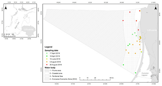
Figure 1.
Lithuanian Baltic Sea. The sampling sites for the Earth Observation (EO) data validation within the water bodies are indicated.
The Lithuanian Baltic Sea is divided into four water bodies following the requirements of the Marine Strategy Framework Directive (MSFD) and the Water Framework Directive (WFD) (Figure 1, Table 1): the Exclusive Economic Zone (EEZ), Territorial Sea, coastal zone, which are subdivided into stony coast in the North, and sandy coast in the South (in this study, this subdivision was not considered) and the plume area.

Table 1.
The division of the Lithuanian Baltic Sea waters into the water bodies and their size.
2.1.2. Ukrainian Black Sea
The Ukrainian sector of the north-western Black Sea is located within the coastline from the Danube Delta to Cape Tarkhankut (Crimea), and represents 25% of the total area of the Black Sea (Figure 2). It is comprised of shallow (average depth of less than 180 m) transitional and coastal water bodies (river plumes, estuaries, and bays), shallows (spits and banks), and indented shores [53]. The geomorphological features determine the extended phytal zones with infralittoral and circalittoral [54]. The main freshwater discharge occurs in the north-western part of the Black Sea [55] as the four major rivers drain here: Danube, Dnieper, Southern Bug, and Dniester. The total average freshwater runoff in the region is 272 km3 year−1, i.e., 80% of the total river flow of the entire Black Sea basin, with the Danube River—the largest European river, representing 61% of the total river flow to the Black Sea [5,56,57]. The river runoff results in considerable desalination zones in the coastal areas with surface salinities ranging from less than 15 PSU in the river influence zone while in the open sea, it reaches about 18–19 PSU [56,58]. These features of desalination and geomorphological heterogeneity of the seabed topologically represented by paleo-valleys and watersheds of flooded paleo-rivers led to the formation of a thermo-haline structure with pycnocline [59]. Winds of north-western, western, and south-western directions, connected with circulation in temperate latitudes of the northern hemisphere predominate in the region [60]. The annual SST cycle range in the Black Sea is around 17 °C with the coldest temperature in winter, i.e., water temperatures in the north-western shelf < 5 °C with the presence of sea ice in some regions, and the warmest temperature of around 25 °C in summer, mainly in July and August [58,61,62]. The dominant phytoplankton include diatoms, dinoflagellates, and coccolithophores [8,63]. Diatoms are the most abundant group, and they typically bloom in spring and early summer. Dinoflagellates are also common, and some species are known to cause harmful algal blooms. In recent years, the mass development of cyanobacteria has caused water blooms in the summer and early autumn to worsen water quality. Dominant species are Dolichospermum affine, Aphanizomenon flos-aquae, Nodularia spumigena, Oscillatoria kisselevii, Spirulina laxissima, and Microcystis aeruginosa [8]. The high variations in Chl-a (0.13–98.7 mg m−3 [64]), TSM (0.3–12.0 g m−3 [18,64]), and CDOM (0.06–2.36 m−1, with an average of 0.46 ± 0.45 m−1 [64]) confirm that the waters of the Ukrainian Black Sea are optically complex. Water transparency in the coastal areas of the sea is primarily defined by the concentration of suspended and dissolved substances and ranges from less than 2 m up to 11 m [65].
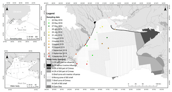
Figure 2.
Ukrainian Black Sea. The sampling sites for EO data validation within the water bodies are indicated. CR—coastal region, CeR—central region, BlS—Black Sea.
The Ukrainian Black Sea is divided into thirty water bodies following the requirements of the MSFD and the WFD. For a better interpretation of the results of this study, several water bodies were merged according to hydrological and geographical features, e.g., coast type, bathymetry, and water regime (Figure 2, Table 2).
Table 2.
The division of the Ukrainian Black Sea shelf waters into water bodies and merged water bodies used in this study for the ecological status assessment.
2.2. Chlorophyll-a Retrieval from Satellite Data
2.2.1. Processors
The first attempt to map chlorophyll-a (Chl-a) concentration in the Lithuanian coastal waters of the Baltic Sea was performed by Vaičiūtė et al. [49]. Cloud-free satellite images of the Medium Resolution Imaging Spectrometer (MERIS) on-board Envisat full spatial resolution (FR, 300 m at nadir) were used. The MERIS sensor operated in the visible and near-infrared spectral range (400 to 900 nm) with a wavelength configuration sensitive to the most important optically active water constituents. MERIS acquired data in 15 spectral bands. In total, five neural network-based processors for optically Case 2 or coastal and inland waters were tested for Chl-a retrieval: FUB (1.2.4 version) [66], Case 2 Regional processor (C2R, 1.4.1 version), Eutrophic lakes processor (Eutrophic, 1.4.1 version) and Boreal lakes processor (Boreal, 1.4.1 version) [67], and standard MERIS Level-2. Chl-a concentrations were validated with in situ data collected in 77 sampling sites during May–September 2010, where Chl-a ranged from 0.69 to 156.18 mg m−3. Results showed that the FUB processor provided the most accurate estimates of the concentration of Chl-a (R2 = 0.69; RMSE = 14.44, N = 56) in comparison with other tested processors [49]. Most importantly, the FUB processor estimated relatively higher Chl-a concentrations ranging from 25 to more than 100 mg m−3 with sufficient accuracy, which often occur in the coastal waters of the Lithuanian Baltic Sea. Therefore, the FUB processor was indicated as the most appropriate approach for the Chl-a concentration retrieval from the MERIS images (more details in [49]).
In this study, we used the Ocean and Land Colour Instrument (OLCI) on-board Sentinel-3A/B images over the Lithuanian Baltic Sea and Ukrainian Black Sea waters. The OLCI sensor operates in the visible and near-infrared spectral range (400 nm to 1020 nm), and acquires data in 21 spectral bands, and has been operating since 2016.
Cloud-free Level-1b Full Resolution (FR, with 300 m pixel size at the nadir) images were downloaded from the Copernicus Open Access Hub (https://scihub.copernicus.eu/, accessed on 7 May 2020). Two neural network-based processors were used to perform the atmospheric correction and retrieve remote sensing reflectance (Rrs) and Chl-a concentration from the Level-1b images: FUB-CSIRO (version 1.0.0.0.5.4) and C2RCC (Case 2 Regional CoastColour, version 1.0). Sentinel-3 Toolbox Kit Module (S3TBX; version 6.0.4) in Sentinel Application Platform (SNAP; version 9.0.) was used to process the Level-1b OLCI images.
Originally, the FUB processor was designed for European coastal waters and uses Level-1b top-of-atmosphere radiances to retrieve Rrs and the concentration of the optical water constituents from the MERIS images [66], and lately, it was adapted for OLCI data and named FUB-CSIRO [68]. The algorithm class is a full spectral physics-based inversion method that performs a pixel-by-pixel direct inversion of the Top of Atmosphere (TOA) signal into spectral remote sensing reflectance Rrs(λ) = LW(λ)/Ed(λ) [sr−1], defined as the ratio of the water-leaving radiance LW(λ) and the downwelling irradiance Ed(λ), with associated sensor and inverse model uncertainties at mean sea level. A set of quality flags generated by FUB-CSIRO was applied to remove image pixels where the inversion of the satellite signal failed, from further processing. A combined valid-pixel expression was constructed to “quality_flags.sun_glint_risk” or “quality_flags.land” or “quality_flags.bright” or “quality_flags.coastline” or “quality_flags.invalid” or “quality_flags.dubious”. The expression allows masking of bright pixels associated with cloud probability, affected by sun glint due to viewing and wind conditions, invalid pixels, i.e., a pixel value is missing either it is out of the instrument swath or due to unusable Level-0 data, and any pixels that are potentially contaminated by a neighbour saturated pixels [69]. In addition, land and coastline pixels were masked as well.
The Case 2 Regional CoastColour (C2RCC) processor, is software for processing Ocean Colour data from different satellite instruments, e.g., OLI, MERIS, MODIS, SeaWiFS, MSI and OLCI [70]. The processor is a further development of the Case 2 Regional Processor (C2R) produced by Doerffer and Schiller [67], which was further modified during the CoastColour project (www.coastcolour.org, accessed on 17 October 2022). In this processor, atmospheric correction is performed and reflectance values are converted into water quality parameters with different neural networks (NNs). The C2RCC processor provides flexibility in adjusting ancillary parameters, e.g., salinity, temperature, ozone, air pressure, and specific IOPs, namely the Chl-specific absorption coefficient and the specific scatter of total suspended matter. In this study, salinity and temperature were regionally adjusted. A combined valid-pixel expression was constructed to “quality_flags.sun_glint_risk” or “quality_flags.land” or “quality_flags.bright” “uality_flags.straylight_risk” or “quality_flags.cosmetic” or “quality_flags.coastline” or “quality_flags.invalid” or “quality_flags.dubious”.
In addition, the Neural Network-based standard Level-2 data (the Sentinel-3 OLCI FR Level-2 water products—OL_2_WFR) were downloaded from the Copernicus Online Data Access (CODA) service. As the outputs, the processor provides Rrs data and the Chl-a products. The images are available for download pre-processed with two established Chl-a algorithms, one based on spectral ratios for open marine water bodies (OC4Me) [71] and the other based on a neural networks (NNs) approach (Case 2 Regional/Coast Color (C2RCC)) for complex water bodies [67]. The latter takes into account light attenuation by phytoplankton pigments, absorption by coloured dissolved organic matter (CDOM), and scattering by suspended particulate matter (SPM), by integrating these bio-optical properties with preceding atmospheric correction to provide an optimal algorithm for Case 2 waters [67]. The OC4Me algorithm originally was developed for Chl-a concentration retrieval in open ocean Case 1 waters, where phytoplankton is the main driver of water optical properties. However, it is also worth testing its performance over the Baltic and Black Seas, which are considered optically complex Case 2 waters due to the presence of high concentrations of CDOM caused by humic-rich water inflow from the rivers, and high concentrations of sediments due to resuspension [72].
In total, three atmospheric correction processors (FUB-CSIRO, C2RCC and standard Level-2), and four Chl-a concentration products (outputs of FUB-CSIRO, C2RCC, Level-2 NN and Level-2 OC4Me) were validated against in situ measured Rrs and Chl-a concentration, respectively. The validation exercise utilized the satellite data constructed by extracting a 3 × 3 pixel window centred on the (Lat/Lon) coordinates of the in situ measurements. In evaluating each 3 × 3 window, the proportion of flagged pixels (invalid data based on processor-specific flags) was calculated. If over 50% of the window pixels were flagged as invalid, the site was excluded from further analysis. For the remaining pixels, the homogeneity was tested according to [73]. The probability of the presence of mixed pixels, adjacency, and the bottom effect in the nearshore zone was solved by the elimination of the distance of 900 m (i.e., three pixels of MERIS and OLCI) from the shoreline in all images. This distance was determined after careful visual inspection of both the RGB composites and reflectance by considering the entire dataset [74,75].
2.2.2. In Situ Data for Validation
In situ data were collected during five field campaigns carried out from April to August 2019 in the coastal waters of the Lithuanian Baltic Sea (see Figure 1). Chl-a data for validation were collected during eleven field campaigns carried out in May 2016 and July-September 2019 in the Black Sea (see Figure 2). Data on the Chl-a concentrations in the Black Sea were obtained from the results of the Black Sea EMBLAS-PLUS project (https://blackseadb.org/, accessed on 14 November 2022).
Chl-a concentration was analysed using the same methodology in both study sites. Water samples were taken from just below the sea surface. Water samples for Chl-a measurement were filtered through glass fibre GF/F filters with a nominal pore size of 0.7 μm and extracted into 90% acetone. Photosynthetic pigments were measured spectrophotometrically and estimated according to the trichromatic method [76,77].
In situ remote sensing reflectance (Rrs) was measured only in the coastal waters of the Lithuanian Baltic Sea. Rrs was acquired in the spectral range of 400–800 nm by the simultaneous measurements of downwelling irradiance, sky radiance, and water leaving radiance, performed with a WISP-3 spectroradiometer [78], and calculated according to Equation (1):
where Lu is the upwelling radiance, Ld—the downwelling radiance, Ed—the downwelling irradiance, ρ—the water surface reflectance factor of 0.028.
2.3. CyaBI Index Calculation
The CyaBI index is based on two parameters: (1) cyanobacterial surface accumulation determined from EO data and (2) in situ determined cyanobacterial biomass. If either parameter does not apply to a specific assessment unit, then only one parameter is used [29]. Originally the inputs to calculate the CyaBI index include the Chl-a concentration as a proxy for cyanobacterial biomass, and turbidity that indicates the presence of dead cyanobacteria derived from satellite data [27]. However, the enhanced turbidity in transitional and coastal waters is strongly caused by outflowing organic and inorganic suspended matter from the rivers or resuspended by strong wind events [49,79]. Therefore, in this study, the CyaBI index was calculated using EO-based Chl-a data, which cover the period from 20 June to 31 August, i.e., the period of typical cyanobacteria occurrence in the Baltic Sea during 2006–2011 (MERIS) and 2016–2019 (OLCI) (Table 3).
Table 3.
The summary of the investigated years and number of available satellite (N) images for coastal water of the Lithuanian Baltic Sea and the Ukrainian Black Sea. The first number indicates the number of available satellite images for Chl-a, and the second number—for SST.
The empirically derived Chl-a concentration maps were classified into four classes of blooming intensity based on the class boundaries proposed by Anttila et al. [27]: 0–11 mg m−3—no algal surface accumulations (0), 11–27 mg m−3—potential algal surface accumulations (1), 28–46 mg m−3—likely algal surface accumulations (2), and >46 mg m−3—evident algal surface accumulations (3).
The remotely sensed daily algal bloom products were first spatially aggregated by calculating a so-called algae barometer value (AB) for each investigated water body. The algae barometer value (Equation (2)) is a weighted sum of the proportion of positive algae bloom estimations in the three potentiality blooming classes (1–3) observed in an MSFD unit [80].
where ntot is the total number of observations, and ncl1, ncl2, and ncl3 are the number of algae bloom cases in the blooming intensity classes 1–3.
According to Anttila et al. [27], a problem in using this method with an extensive number of observations available from satellite data (i.e., pixels) was detected. Even a single pixel with a positive algae observation increases the daily algae barometer to a value above zero and affects the bloom characteristics estimation. To tackle this problem, very low algae barometer values (<0.002) were set as zero under the assumption that these values do not represent significant algal blooms or, more likely, are caused by erroneous observations (e.g., caused by small clouds).
As indicative variables for the CyaBI index, three bloom characteristics were defined: (i) seasonal bloom volume, (ii) duration of the algal surface accumulation period, and (iii) bloom severity. These characteristics were estimated for each water body (see Table 1 and Table 2) and year. The cumulative proportion of the observations was derived from the daily AB values using the empirical cumulative distribution functions (ECDF; more details in [81]). Seasonal bloom volume was determined from the area above the ECDF functions. The duration of the algal surface accumulation period was represented by the percentage of observations with algae barometer values above 0.002, and the bloom severity was determined based on the 90th percentile of the algae barometer observations.
The CyaBI index combines these indicative variables by averaging the normalised time series from each of them. The included variables were considered equally important. The time series of indicative variables describing the bloom characteristics were normalised according to Equation (3).
where Pnorm,y is the normalized value of a parameter for year y and Py is the actual parameter value for the year. Pmin and Pmax are the minimum and maximum values of the time series with annual time steps.
The ecological status was assessed considering the Good Ecological Status (GES) threshold values of the CyaBI index provided in HELCOM [29].
2.4. SST Retrieval
MODIS Level-2 SST products (spatial resolution of about 1 km) were retrieved from the moderate resolution imaging spectroradiometer (MODIS) on-board Terra and Aqua from the NASA OceanColor website (http://oceancolor.gsfc.nasa.gov/, accessed on 8 June 2023). There are typically about 2 to 4 MODIS Terra/Aqua observations of the study region (both, in the Baltic Sea and the Black Sea) per day. Aqua provides observations ca. 10–12 UTC in the daytime and 00–02 UTC at night, while Terra provides observations at around 08–11 UTC in the daytime and 19–21 UTC in the evening. The validation of the MODIS SST product against in situ observations showed a very good agreement between satellite and conventional in situ measurements in the Baltic Sea (with R2 not less than 0.78, more details in [50]) and in the Black Sea (with R2 not less than 0.83, more details in [82].
To assess the SST changes within the presence and intensity of the cyanobacteria blooms in the Baltic Sea, six out of ten investigated years with the highest number of cloud-free SST maps were selected (see Table 3). The images were selected at the nearest possible time to the satellite retrievals of Chl-a. Only in a few cases, due to the absence of cloud-free daytime SST maps, night-time SST imagery of the same day was used. The mean SST values were extracted overlaying the CyaBI maps comprising four classes of blooming intensity and according to the determined water bodies in the Lithuanian Baltic Sea and the Ukrainian Black Sea. The differences in SST were calculated between class 1, class 2, class 3 and class 0, which refers to no algal surface accumulations over the water.
2.5. Statistical Data Analysis
For analysing the difference between satellite-derived and in situ measured Chl-a concentration the coefficient of determination (R2), the root mean square error (RMSE, Equation (4)), the normalized root mean square error (NRMSE, Equation (5)), and the mean bias error (bias) were used.
where xin situ is the field measurement, ysat—the satellite estimation, N—the total number of observations, and xin situ max and xin situ min—the maximum and minimum Chl-a concentration from the field measurements.
The spatial-temporal patterns of the seasonal bloom volume, duration of the algal surface accumulation period, bloom severity, and CyaBI index in the Baltic Sea and the Black Sea were assessed using the Generalized Additive Modelling (GAM) or the Generalized Additive Mixed Modelling (GAMM). Each algal parameter was a response variable in the model, where the interaction effect of studied years and the water bodies (as a nominal explanatory variable) was selected as a smoothing explanatory variable, and the variable of water bodies was also included separately. The penalized cyclic cubic smoothing term was selected for the smoothing explanatory variable with 4 degrees of freedom. Based on the Akaike’s Information Criterion (AIC), the Gaussian or scaled t (identity link) distribution was selected in the models, which were performed with the ‘mgcv’ package for R [83]. Due to the unequal variances between the water bodies, ‘varIdent’ variance structure was also tested in the GAMM models by AIC using the ‘nlme’ package for R [84]. For each model, the assumptions of the normal distribution, homogeneity and autocorrelation of residuals were checked, respectively, by a normal Q-Q plot, a plot of residuals vs. fitted values, and a residual autocorrelation plot by ‘acf’ function [85].
The GAMM was also used for the testing of significance of SST trends along the CyaBI classes. The SST was selected as a response variable in the model, where the interaction effect of CyaBI and the water bodies was selected as a fixed smoothing explanatory variable (smoothing term with penalized cyclic cubic and 4 degrees of freedom), the interaction effect of months and years was selected as a random smoothing explanatory variable (smoothing basis with “re”), while the variable of the water bodies was included separately. The proportion of variance explained (deviance) by the GAM model was determined. All statistical analyses were performed in R [86] using RStudio [87].
3. Results
3.1. Validation of Rrs and Chl-a Concentration
The remote sensing reflectance data (Rrs) were available only from the coastal waters of the Lithuanian Baltic Sea. The spectral shape of reflectance derived by the FUB-CSIRO processor is reasonably in line with the in situ measurements (Figure 3). A slight underestimation can be observed at 560 nm. Relatively higher variability of Rrs across the sites with higher underestimation at 560 nm was observed after the application of C2RCC to OLCI data. The Level-2 images in some cases provided negative values of Rrs, especially in the blue and red-NIR sections of the spectrum.
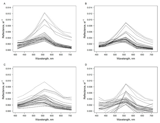
Figure 3.
Remote sensing reflectance (sr−1) measured in situ (A) and retrieved from the OLCI images after application of FUB-CSIRO (B) and C2RCC (C) processors, and acquired from the Level-2 images (D) over the coastal waters of Lithuanian Baltic Sea in April–August 2019. In total, 35 spectra are plotted. Only the bands common to all processors are plotted, i.e., bands centred at 412, 443, 490, 510, 560, 620, 665 and 708 nm wavelengths.
Based on R2, RMSE, NRMSE and bias, the lowest agreement of Rrs corresponded to the blue bands (Figure 4). Particularly for bands centred at 412 and 443 nm, the FUB-CSIRO processor showed the lowest RMSE and NRMSE with a slight underestimation, while the C2RCC processor showed an overestimation. The agreement of Rrs at 490 nm was the highest for FUB-CSIRO with a slight underestimation, while the C2RCC and Level-2 processors showed the same tendency as for bands centred at 412 and 443 nm. At the green to NIR section of the spectrum, the agreement of Rrs was the highest after the application of the FUB-CSIRO processor. This processor underestimated more than the C2RCC processor for the bands starting from 560 nm, whereas the highest underestimation was of the Level-2 images.
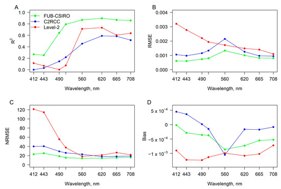
Figure 4.
Agreement, based on (A) the coefficient of determination (R2), (B) the room mean square error (RMSE) in sr−1, (C) the normalised root mean square error (NRMSE) in %, and (D) the mean bias error (Bias) in sr−1, between remote sensing reflectance measured in situ and retrieved after the application of FUB-CSIRO, C2RCC, and acquired from the Level-2 images for certain wavelengths.
In situ measured Chl-a concentration levels ranged from 1.41 to 22.47 mg m−3, with a mean of 7.15 ± 6.18 mg m−3 during the period of sampling for the OLCI data validation in the coastal waters of the Lithuanian Baltic Sea. The highest (22.47 mg m−3) concentration was determined near the outflow of the Curonian Lagoon in August 2019. Relatively lower Chl-a concentration was measured in the Black Sea, ranging from 0.20 to 29.83 mg m−3, with a mean of 3.15 ± 6.25 mg m−3. The highest (29.83 mg m−3) concentration was determined in the north-western part of the Black Sea near the Dnipro River outflow in September 2019.
The best fit between in situ and estimated Chl-a concentration considering two datasets (separately and combined) was found for the FUB-CSIRO processor (Figure 5, Table 4). A relatively good fit was observed for the C2RCC processor, although with higher RMSE and NRMSE values than for the FUB-CSIRO processor. An obvious underestimation of higher than 10 mg m−3 Chl-a concentration was determined by the C2RCC processor and standard Level-2 NN products. An evident overestimation of Chl-a concentration was determined for standard Level-2 OC4Me products, and on average 27% of the data was discarded due to flagged pixels. The validation results of four processors applicable to OLCI data for Chl-a concentration retrieval indicated that the FUB-CSIRO processor is mostly appropriate for further use.
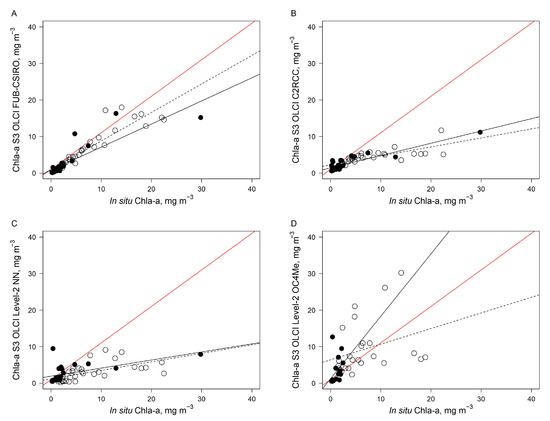
Figure 5.
Relationship between Chl-a concentration derived from OLCI/Sentinel-3 data after application of FUB-CSIRO (A), and C2RCC (B) processor, and acquired from the Level-2 NN (C) and OC4Me (D) products with in situ measured Chl-a. In situ data were collected in April–August 2019 in the coastal waters of the Lithuanian Baltic Sea (open circles), and in May 2019 and July–September 2019 in the Black Sea (black circles) (see Figure 1 and Figure 2). The dashed line indicates the linear regression fit for the Baltic Sea data, the black line indicates the linear regression fit for the Black Sea data, and the red line represents a 1:1 fit. The regression statistics are provided in Table 4.
Table 4.
Regression equations, the coefficient of determination (R2), the root mean squared error (RMSE) in mg m−3, and the normalized root mean square error (NRMSE) in % of investigated processors applied to the OLCI data for the Chl-a concentration retrieval in the case of the Baltic Sea, the Black Sea, and combined datasets. N—number of measurements.
After the application of the FUB processor to the MERIS images and the FUB-CSIRO processor to the OLCI images from the Lithuanian Baltic Sea, the highest values of Chl-a were recorded close to the outlet of the Curonian Lagoon and along northern coastal waters (Figure 6). Moderately high Chl-a concentrations were determined in the open water, while the lowest values were observed in the Territorial Sea and along southern coastal waters. In the Ukrainian Black Sea, the highest Chl-a was determined near the outflows of the biggest rivers (Danube, Dniester and Dnieper), while the lower concentrations were in the shelf zone and open waters.
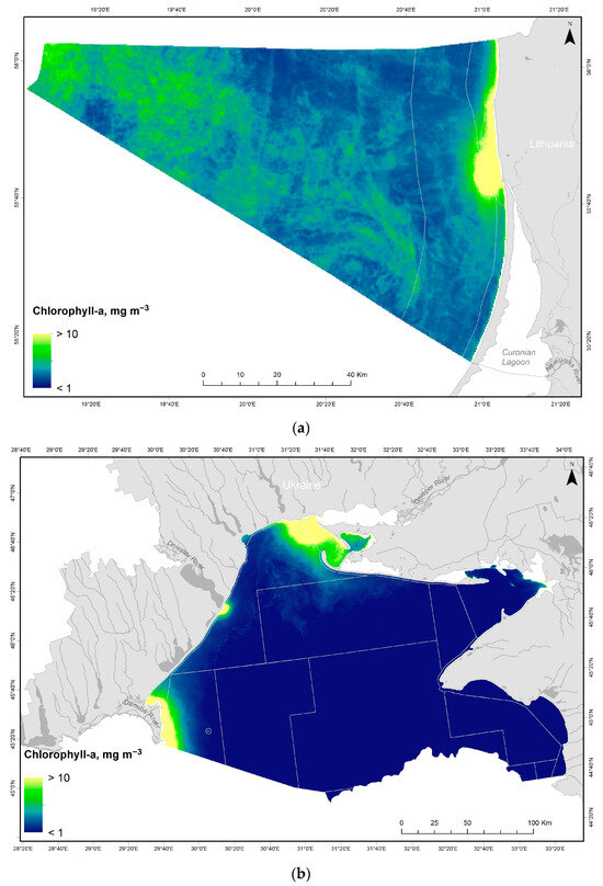
Figure 6.
Spatial distribution of the mean Chl-a concentration (mg m−3) during 2006–2019 (the period of 2012–2015 is not covered due to the lack of satellite data) in the Lithuanian Baltic Sea (a) and the Ukrainian Black Sea (b). The water bodies are indicated by grey lines.
3.2. Cyanobacteria Blooms in the Lithuanian Baltic Sea: Inter-Annual Variability and Spatio-Temporal Trends
In the Lithuanian Baltic Sea, the least affected water bodies by cyanobacteria blooms were the Exclusive Economic Zone (EEZ) and Territorial Sea, where >80% of investigated cases were without blooms (Figure 7). In the plume area and coastal waters, the cyanobacteria blooms were not observed in <40% of investigated cases, except in 2018 and 2019, where the tendency was similar to the EEZ and Territorial Sea. The potential surface accumulations (class 1), where the Chl-a concentration ranged from 11 to 27 mg m−3, were determined in the EEZ, coastal waters and the plume area in 2006, while in 2010, 2011 and 2017, the potential surface accumulations were indicated in the Territorial Sea and coastal region, including the plume area. A significant decrease in the presence of potential surface accumulations was observed during 2018 and 2019. In total, the potential surface accumulations were present in <40% of investigated cases. A similar tendency was determined for the likely algal surface accumulations (class 2), where the Chl-a concentration ranged from 28 to 46 mg m−3. The evident algal surface accumulations (class 3), defined by the Chl-a concentration of >46 mg m−3, were more frequent (around 40% of total investigated cases) in the EEZ and coastal region including the plume area during 2006, 2010 and 2011, while in 2017 and 2019 the evident algal surface accumulations were more present in the EEZ, and significantly rare in the coastal region. In 2018, no evident algal surface accumulations were determined.
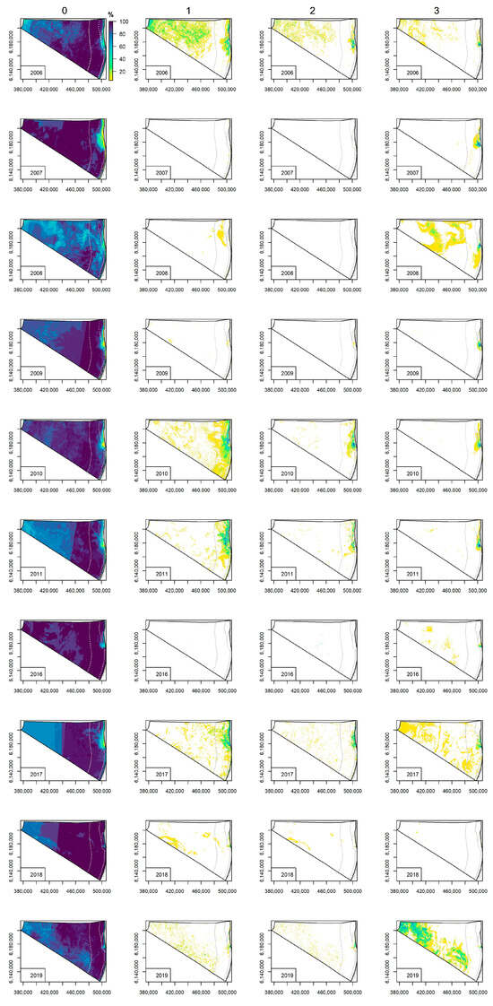
Figure 7.
Spatial distribution of relative occurrence (from the total number of satellite images available for each investigated year) of cyanobacteria bloom intensity classes derived from the Earth Observation data in the Lithuanian coastal waters of the Baltic Sea. Class 0 indicates no algal surface accumulations present, 1—potential algal surface accumulations, 2—likely algal surface accumulations, and 3—evident algal surface accumulations. The water bodies are indicated by grey lines.
In the plume area, the blooms covered on average 36 ± 28%, i.e., 33 ± 26 km2, of the total plume area (Figure 8). The blooms covered >80% of the surface during 2007, and in June–July during 2009 and 2010, with a relatively equal proportion of all three algal surface accumulations classes. During 2016–2017, the blooms covered approximately 60% of the surface; however, the class 1, indicating the potential algal surface accumulations, was mainly determined. During 2018–2019, the blooms’ coverage significantly decreased up to 88 ± 11 km2 and 11 ± 15 km2, respectively, and only sporadically reached up to 40% of the total plume area.
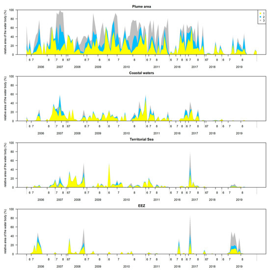
Figure 8.
Temporal variability of relative bloom area from the total area of the water body (provided in Table 1) in the Lithuanian coastal waters of the Baltic Sea during the investigated years. Class 0 indicates no algal surface accumulations present, 1—potential algal surface accumulations, 2—likely algal surface accumulations, and 3—evident algal surface accumulations.
In the coastal waters, the blooms covered on average 8 ± 12%, i.e., 23 ± 32 km2, of the total coastal waters area (Figure 8). The blooms covered >40% of the surface during 2007 and 2010. Throughout the entire investigation period, the most dominant was class 1 indicating the potential algal surface accumulations. The lowest bloom coverage was determined during 2018–2019 with 3 ± 2 km2 and 1 ± 3 km2, respectively.
In the Territorial Sea, the blooms covered on average 5 ± 10%, i.e., 74 ± 152 km2, of the total Territorial Sea area (Figure 8). In contrast to the plume area and the coastal waters, the largest blooms were recorded in 2008 and 2017, where the area covered by cyanobacteria accumulations reached 60% and 80%, respectively, with a relatively equal proportion of all three classes of algal surface accumulations.
In the Exclusive Economic Zone (EEZ), the blooms covered on average 5 ± 13%, i.e., 196 ± 566 km2, of the total EEZ area (Figure 8). The largest blooms covering >40% of the surface were recorded in 2006 and 2008, and in contrast to the plume area and the coastal waters, in 2016, 2017 and 2019, where the bloom coverage reached up to 1500, 3900 and 2300 km2, respectively. A relatively equal proportion of all three classes of algal surface accumulations was determined.
3.3. Cyanobacteria Blooms in the Ukrainian Black Seas: Inter-Annual Variability and Spatio-Temporal Trends
In the Ukrainian Black Sea, the least affected areas by cyanobacteria blooms were the coastal region of the south-western part and shelf zone of Crimea, the mixing zone of the shelf (except 2009), the central region of the shelf and open sea, where in >80% of investigated cases the blooms were not observed (Figure 9). In the coastal region with and without riverine influence, the blooms were not observed in <40% of investigated cases, except in 2016 and 2017.
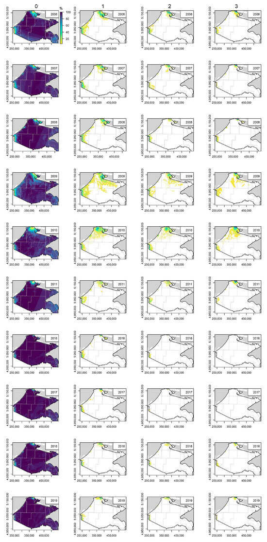
Figure 9.
Spatial distribution of relative occurrence (from the total number of satellite images available for each investigated year) of cyanobacteria bloom intensity classes derived from the Earth Observation data in the Ukrainian shelf of the Black Sea. Class 0 indicates no algal surface accumulations present, 1—potential algal surface accumulations, 2—likely algal surface accumulations, and 3—evident algal surface accumulations. Water bodies are indicated by grey lines.
The potential surface accumulations (class 1) were determined in all coastal regions, in the shelf zones with riverine influence and the mixing zone of the shelf in 2009–2011, and the central region of the shelf in 2009 (Figure 9). A similar tendency was determined for the likely algal surface accumulations (class 2) and the evident algal surface accumulations (class 3). Since 2011, with an evident decline in potential, likely and evident algal surface accumulations were determined in the coastal region without the riverine influence.
In the coastal region with the riverine influence, the blooms covered on average 29 ± 20%, i.e., 362 ± 252 km2, of the total area (Figure 10). The blooms covered approximately 80% of the surface during 2006, 2008 and 2009, with a relatively equal proportion of all three classes of algal surface accumulations. Since 2016, the bloom coverage has decreased twice.
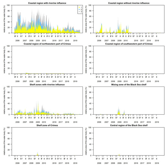
Figure 10.
Temporal variability of relative bloom area from the total area of the water body (provided in Table 2) in the Ukrainian coastal waters of the Black Sea during the investigated years. Class 0 indicates no algal surface accumulations present, 1—potential algal surface accumulations, 2—likely algal surface accumulations, and 3—evident algal surface accumulations.
In the coastal region without the riverine influence, the blooms covered on average 4 ± 8%, i.e., 12 ± 23 km2 of the total area of the unit, with a clear dominance of the class 1 indicating the potential algal surface accumulations (Figure 10). Similarly to the coastal region with the riverine influence, the blooms coverage decreased starting from 2011 in this area (up to 6% of the total area), while the blooms covered up to 40%, i.e., 22 ± 28 km2, of the surface during 2006–2010.
In the coastal regions of the north-western parts of Crimea, the blooms covered the surface up to 4% (up to 60 km2) of the total area of the unit (Figure 10). The blooms rarely occurred in the coastal region of the south-western parts of Crimea.
In the shelf zone with the riverine influence, the blooms covered on average 6 ± 7%, i.e., 420 ± 494 km2, of the total area of the unit (Figure 10). Similarly to the coastal region of the Black Sea with the riverine influence, the blooms covered more than 20% of the surface during 2006–2011, with a relatively equal proportion of all three classes of algal surface accumulations. While since 2016 the blooms mean coverage decreased up to threefold (2 ± 2%).
In the mixing zone of the Black Sea shelf, the shelf zone of Crimea and the central region of the shelf, the blooms rarely covered the surface, except in 2009 and 2010, while no surface blooms were determined in the open Black Sea (not shown in Figure 10).
3.4. Algal Bloom Characteristics and Ecological Status Assessment in the Baltic and Black Seas Using CyaBI
The seasonal bloom volume in the Lithuanian Baltic Sea depended on the zones and years (Figure 11). The mean seasonal bloom volume was significantly higher (0.91 ± 0.29) in the plume area (F = 3.96, df = 3.00, p = 0.02) than in the coastal zone, Territorial Sea and EEZ, where the mean seasonal bloom volume was with relatively high variation (respectively, 0.36 ± 0.28, 0.38 ± 0.47 and 0.45 ± 0.60). In these areas, exceptionally high values of seasonal bloom volume were in 2017 and also in 2010 in the coastal waters, in 2008 in the Territorial Sea and EEZ, and in 2019 in EEZ.
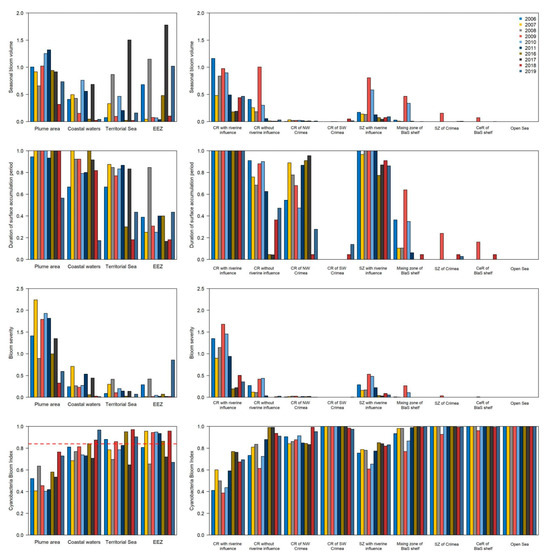
Figure 11.
Spatial-temporal changes (different years and areas) of algal bloom characteristics in the Lithuanian Baltic Sea (left panel of the figure) and the Ukrainian Black Sea (right panel of the figure): seasonal bloom volume, duration of the algal surface accumulation period, bloom severity, and CyaBI index. The red dotted line indicates a good ecological status (GES = 0.84) threshold value determined for the Eastern Gotland Basin of the Baltic Sea which includes the Lithuanian Baltic Sea [29].
In the Black Sea, the highest mean seasonal bloom volume (0.61 ± 0.23) was in the coastal zone with riverine influence, followed by the coastal zone without riverine influence and the shelf zone with riverine influence (respectively, 0.23 ± 0.31 and 0.22 ± 0.26) (Figure 11). Other investigated regions were characterized by relatively lower bloom volume values (<0.07). Negative temporal trends of seasonal bloom volume in the coastal zone with and without riverine influence were significant (respectively, F = 9.61, edf = 1.00, p < 0.01 and F = 4.21, edf = 1.00, p = 0.04).
Algal surface accumulations were present through the entire analysed period in the plume area of the Lithuanian Baltic Sea (Figure 11) during the majority of investigated years (F = 0.96, edf = 1.00, p = 0.34). The algal surface accumulations decreased towards the offshore waters, where they were present in only one-third (0.36 ± 0.19) of the analysed period in the EEZ (except in 2008). A significant decrease in the algal surface accumulation period was determined in the Territorial Sea since 2016 (F = 7.54, edf = 1.33, p = 0.01).
In the Ukrainian Black Sea, algal surface accumulations were present throughout the entire analysed period in the coastal waters with an influence of the riverine waters during all investigated years (F = 0.00, edf = 1.00, p = 1.00) (Figure 11). Relatively shorter mean periods of the algal surface accumulation (0.57 ± 0.33) were determined in the coastal waters without an influence of the riverine waters with a significant decrease since 2011 (F = 25.83, edf = 2.90, p < 0.01). On the opposite, relatively longer periods of algal surface accumulation (0.64 ± 0.30) were determined in the coastal region of NW of Crimea during 2016–2017, and a significant decrease was observed since 2018 (F = 10.29, edf = 2.90, p < 0.01). The algal surface accumulations did not significantly affect the rest of the regions, although there was a marginally significant negative trend since 2016 in the shelf zone of the Black Sea with riverine influence (F = 3.38, edf = 1.00, p = 0.07).
The highest mean bloom severity (1.33 ± 0.62) was determined in the plume area of the Lithuanian Baltic Sea with extreme conditions during 2007 (Figure 11). The bloom severity significantly decreased since 2016 (F = 13.57, edf = 2.18, p < 0.01). In contrast, the mean bloom severity was significantly lower (<0.28) in the rest of the investigated water bodies (F = 49.02, edf = 3.00, p < 0.01). A similar tendency was determined in the Ukrainian Black Sea, where the highest mean bloom severity (0.87 ± 0.54) was in the coastal region with the riverine influence, where a significant decrease in severity was observed since 2016 (F = 67.24, edf = 2.93, p < 0.01). Other investigated regions were characterized by relatively lower bloom severity (<0.14) except coastal regions without riverine influence and the shelf zone of the Black Sea with riverine influence. In the latter regions, significant negative trends were determined since 2016 (respectively, F = 9.22, edf = 1.00, p < 0.01 and F = 6.34, edf = 2.25, p < 0.01).
The lowest mean CyaBI (0.55 ± 0.13) was determined In the plume area of the Lithuanian Baltic Sea (Figure 11), where it significantly increased since 2018 (F = 29.36, edf = 2.93, p < 0.01). CyaBI values were lower than the GES threshold of 0.84, therefore, it corresponded to the bad ecological status. The good ecological status in the coastal waters was reached during the latest investigated years (i.e., 2016, 2018 and 2019), while in the Territorial Sea—during 2006, 2009, 2016, 2018 and 2019. The good ecological status in EEZ was determined during most of the investigated years, except 2006, 2009, 2017 and 2019.
In the Ukrainian Black Sea, the lowest mean CyaBI (0.58 ± 0.14) was in the coastal region with riverine influence, followed by the shelf zone with riverine influence, the coastal region without riverine influence and the NW of Crimea. In the first two regions, statistically significant increasing linear trends of CyaBI were determined (respectively, F = 15.14, edf = 1.00, p < 0.01 and F = 10.27, edf = 1.00, p < 0.01), while a significant decrease in CyaBI was recorded since 2018 (F = 29.36, edf = 2.93, p < 0.01). A good ecological status could be considered in the rest of the investigated regions since the CyaBI values were close to 1 (Figure 11).
3.5. SST Variability in the Presence of Cyanobacteria Bloom
In general, the mean SST determined in the Lithuanian Baltic Sea waters (approx. 20 °C) was approximately lower by 5 °C than in the Ukrainian Black Sea waters with a mean of approx. 25 °C. In the Lithuanian Baltic Sea, the mean SST temporal pattern was usually with the highest SST in the middle of July (Figure 12). Intensive cyanobacteria blooms significantly enhance the short-term increase in SST compared to surrounding waters by the mean of 0.64 ± 0.68 °C, with a maximum of 4.50 °C, in the Lithuanian Baltic Sea, and by the mean of 0.70 ± 0.73 °C, with a maximum of 7.03 °C in the Ukrainian Black Sea. Relatively high mean differences in SST (>2 °C) were observed between the areas of mainly class 2 and class 3 of cyanobacteria bloom intensity (derived from the EO data) and the areas with no algal surface accumulations present. These differences were recorded mainly during June-July in the plume and coastal area, whereas the mean differences in SST between cyanobacteria bloom intensity classes and areas without cyanobacteria blooms recorded were significantly lower in the rest of the water bodies. There were significantly lower mean differences in SST (>−2 °C) in the coastal area in July 2018.
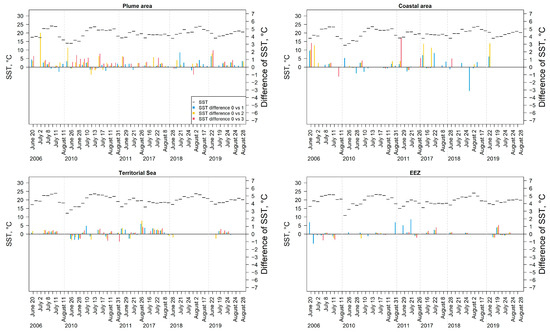
Figure 12.
Temporal changes in the mean SST and the mean difference in SST between the areas, where cyanobacteria blooms were recorded (class 1–3) and the areas with no algal surface accumulations present as derived from the Earth Observation data in different water bodies in the Lithuanian waters of the Baltic Sea.
In the Black Sea, the mean SST temporal pattern was usually with higher SST at the end of July (Figure 13). Relatively high mean differences in SST (>2 °C) were observed between the areas of mainly class 2 and class 3 of cyanobacteria bloom intensity (derived from the EO data) and the areas with no algal surface accumulations present mainly during July–August in the coastal region with and without riverine influence, and coastal region of NW Crimea. Meanwhile, the mean differences in SST were significantly lower in the rest of the water bodies. There were significantly lower mean differences in SST (>−2 °C) in the coastal region and shelf zone with riverine influence.
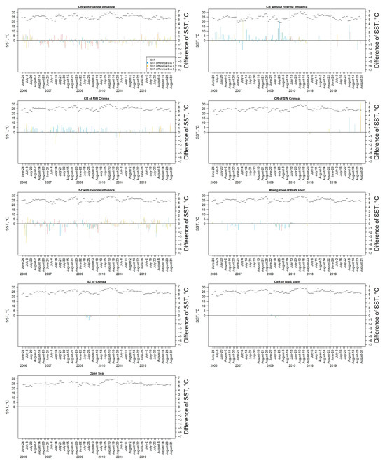
Figure 13.
Temporal changes in the mean SST and the mean difference in SST between the areas, where cyanobacteria blooms were recorded (class 1–3) and the areas with no algal surface accumulations present as derived from the EO data in different water bodies in the Ukrainian Black Sea.
The GAM models explained 69% and 53% of the variance (deviance) of SST, respectively, in the Lithuanian Baltic Sea and the Ukrainian Black Sea. In the Baltic Sea, significant positive linear trends of SST along the increasing CyaBI class (Figure 14A) were determined in the plume and EEZ (respectively, F = 10.70, edf = 1.00, p < 0.01 and F = 5.46, edf = 1.00, p = 0.02), while the significance of the trend in the coastal waters was marginal (F = 4.00, edf = 1.00, p = 0.05). In the Black Sea, significant nonlinear trends of SST along the increasing CyaBI class (Figure 14B) were determined in the coastal zone without riverine influence and SW of Crimea (respectively, F = 4.20, edf = 1.96, p < 0.01 and F = 3.25, edf = 1.76, p = 0.03). The significance of the negative trend in the mixing zone of the Black Sea shelf was marginal (F = 3.63, edf = 1.13, p = 0.06).
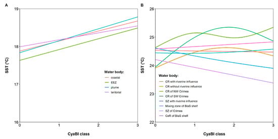
Figure 14.
GAM fitted values of SST for CyaBI classes in different water bodies of the Lithuanian Baltic Sea waters (A) and the Ukrainian Black Sea (B).
From several satellite SST maps (Figure 15A–F), it can be seen that the Lithuanian Baltic Sea areas under the influence of algae accumulations are characterized by higher temperatures compared to those with no algae accumulations present. In the Territorial Sea, the highest CyaBI values were typically observed in the Curonian Lagoon plume zone together with the areas in a close vicinity to the coast (Figure 15B,D). In turn, these areas were distinguished from the surrounding waters by higher water temperature which was up to 3 °C higher in the zones with evident algal accumulations (class 3) compared to the zones with no algal surface accumulations present (class 0). A similar pattern was also observed in the EEZ. On 22 July 2017, the evident algal surface accumulations covered only a small part of EEZ, nevertheless, the difference between average SST in class 3 and class 0 zones was around 0.9 °C. On 19 July 2019, the evident algal surface accumulations (class 3) covered a significant part of the EEZ and in this case, the SST difference reached about 1.4 °C (Figure 15F).
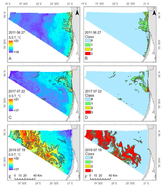
Figure 15.
Examples of the SST (A,C,E) and four classes of blooming intensity (B,D,F) spatial distribution in the Lithuanian Baltic Sea during 27 June 2011, 22 July 2017 and 19 July 2019.
In the Ukrainian Black Sea, water temperature differences due to the presence of algae accumulations were not as significantly pronounced as in the Lithuanian Baltic Sea. The spatial patterns of decreased SST and increased CyaBI were observed under the influence of upwelling events in the coastal regions (Figure 16A–D). In the example provided for 4th August 2010, positive water temperature variations were associated with increased Chl-a concentration expressed as CyaBI class 1–3 in the coastal region with the influence of the Dnieper River and the Danube River (Figure 16E,F).
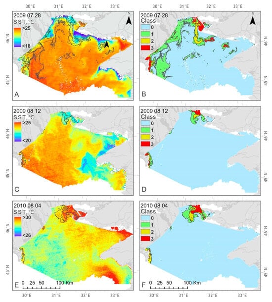
Figure 16.
Examples of the SST (A,C,E) and four classes of blooming intensity (B,D,F) spatial distribution in the Ukrainian Black Sea on 28 July 2009, 12 August 2009 and 4 August 2010.
4. Discussion
4.1. The Remote Sensing of Chl-a Concentration: The Importance of the Accuracy
In general, Chl-a concentration is a variable that is primarily sensed remotely which can provide an understanding of ongoing eutrophication in a waterbody, determine its productivity, and reflect its health. It is therefore used as an indicator for both the assessment and management of ecological status. However, to ensure the accuracy of Chl-a mapping using remote sensing data, it is crucial to carefully select the most appropriate approach for processing the data while considering the uncertainties that may arise and significantly impact the overall accuracy. Accurate atmospheric correction of satellite optical imagery over the water bodies is a prerequisite for quantitative aquatic remote sensing and remains a key challenge in inland and coastal waters, especially in the Baltic Sea [88,89]. This is due to numerous confounding factors such as the complexity of water optical properties, the surface glint, the heterogeneous nature of atmospheric aerosols, and the proximity of bright land surfaces. This combination of factors makes it difficult to retrieve accurate information about the system observed. Therefore, validation of the approaches for satellite data processing and algorithms is an important step because their accuracy directly determines the accuracy with which satellite ocean colour products, e.g., Chl-a concentration, can be derived from subsequent processing using atmospherically corrected reflectance spectra as input. The overall accuracy of an AC algorithm is usually determined by comparison of the satellite-derived reflectance against in situ radiometric observations. This match-up approach quantifies the mean retrieval accuracy ideally across a large number of concurrent in situ and satellite observations. In this study, we have investigated the performance of three commonly used processors (FUB-CSIRO, C2RCC and Neural Network-based standard Level-2 data) to retrieve the Rrs only in the Lithuanian Baltic Sea waters, since in situ radiometric observations were not available for the Ukrainian Black Sea waters. To the best of our knowledge, this is the first study, where the performance of the FUB-CSIRO processor was tested over the Baltic and Black Seas. The spectral shape of the derived reflectance by FUB-CSIRO was reasonably in line with the in situ measurements with a slight underestimation at 560 nm. The lowest agreement was determined in the blue portion of spectra, while at the green to NIR section of the spectrum the agreement was highest (R2 ranged from 0.79 to 0.90). Similar results were obtained by Schroeder et al. [68] over the coastal waters of the Great Barrier Reef (Australia), and based on our search, this has been the only study where FUB-CSIRO was successfully applied to OLCI data. The other investigations were focused on the validation of the FUB processor (plugin for the BEAM VISAT platform) applicable to MERIS images (e.g., [17]), and determined that the FUB processor provided the consistent spectral shape, although slightly underestimated the reflectance in all bands compared to sea-truthing data. Considering that the former FUB is the follow up processor to the FUB-CSIRO, and MERIS is the follow up mission to OLCI, all the findings confirm that this approach is suitable for the optical remote sensing data processing over the optically complex coastal waters with a wide range of in-water constituents.
In our study, the lowest agreement nearly for every investigated band was found for the C2RCC processor, with the R2 ≤ 0.6 of the bands starting from 560 nm. Kutser et al. [21] demonstrated that the C2RCC processor applied to OLCI data is capable of producing quite reasonable reflectances in the Estonian Baltic Sea waters. The exception might be relatively dense cyanobacterial bloom areas due to uncorrected C2RCC-derived Rrs at red/near-infrared wavelengths [90,91]. The same processor was evaluated in the Black Sea by Grégoire et al. [58] against Rrs measured by the two Black Sea Aeronet-OC stations “Gloria” and “Galata” located in the western part. The agreement between in situ measured and retrieved from OLCI after application of C2RCC Rrs was significantly high for all investigated bands (i.e., 413, 443, 490, 560 and 665 nm), where R2 ranged from 0.64 to 0.90 for the blue bands, and R2 ranged from 0.83 to 0.88 for green and red bands. The contradictory results related to atmospheric correction performance by C2RCC are most likely linked to the optical complexity, especially in coastal areas, where influence by CDOM is high, and the spatio-temporal variations. This highlights a demand for further and more detailed analysis of both studied seas.
In our study, we demonstrate that the atmospheric correction of OLCI Level-2 products was not suitable in the Lithuanian Baltic Sea conditions, since negative values of Rrs, in particular in the blue and red-NIR sections of the spectrum were recorded. These findings were provided also by Kutser et al. [21], where in the case of relatively clear open Baltic Sea waters the reflectances were negative in the blue bands in such CDOM-rich waters. The study also discovered that in the presence of algal bloom and due to the increase in phytoplankton biomass a larger portion of the OLCI reflectance spectra becomes negative.
In general, our results showed that Chl-a retrieved from OLCI data after application of the FUB-CSIRO processor showed a good agreement with in situ Chl-a measurements in both the Lithuanian Baltic Sea and the Ukrainian Black Sea waters. To our best knowledge, this is the first study, where the FUB-CSIRO processor was tested for the Chl-a retrieval in the Baltic Sea and the Black Sea waters, therefore the only comparison of the results can be performed considering the previous investigations focused on the validation of Chl-a after application of the FUB processor applicable to MERIS images. The previous studies performed in the Lithuanian Baltic Sea coastal waters showed a good agreement between Chl-a measured in situ and derived from the MERIS data after application of the FUB processor, especially in the open sea and in the plume area, where relatively high concentration of pigments and other in-water constituents occurred [49]. The performance of the FUB processor to retrieve the Chl-a concentration after application to the MERIS data was tested in Skagerrak [92] and in the north-western part of the Baltic Sea [93]. Similarly, the study in Skagerrak demonstrated the ability of the FUB processor to retrieve well Chl-a. Kratzer et al. [93] and Beltrán-Abaunza et al. [17] found that the Chl-a concentration retrieved after the application of the FUB processor to the MERIS data had the lowest bias. These promising results from the validation suggest that the FUB processor could be used as a common tool for monitoring the spatial distribution of Chl-a in the Baltic Sea and the Black Sea. The success of both the FUB processor for MERIS data and the FUB-CSIRO processor for the OLCI data could also support the retrieval of Chl-a time series that covers the period of 2002–2012 (MERIS mission) and 2016-up today (OLCI mission).
Although the low values of the Chl-a concentration retrieved from the OLCI data after application of the C2RCC processor provided reasonable results, the processor strongly underestimated the Chl-a concentration higher than 10 mg m−3 in both the Lithuanian Baltic Sea and the Ukrainian Black Sea waters. The same results were obtained in the north-western part of the Baltic Sea [22,88] and Estonian Baltic Sea waters [21], where the processor underestimated Chl-a above the same threshold, or provided a poor agreement with in situ measured Chl-a. Better results were obtained by Soomets et al. [23], where the Chl-a concentration measured in situ and derived after the application of the C2RCC processor to the OLCI data was in relatively good agreement (R2 = 0.55) indicating that the performance of the processor should be tested further more in details, especially due to the possibility for modification of the C2RCC parameters to better reflect local conditions generating the Chl-a product [88]).
The validation of two standard Chl-a concentration products (Level-2 NN and OC4Me) provided by EUMETSAT showed that the fit between satellite derived and in situ measured values was in moderate to a poor agreement for both, the Lithuanian Baltic Sea and the Ukrainian Black Sea waters. Similar findings were described in Soomets et al. [23] over the Estonian Baltic Sea waters, where the R2 between in situ measured and standard Level-2 NN Chl-a product was 0.39, and the OC4Me product—0.02. In addition, a significant number of pixels (up to 60%) usually are flagged in the standard Level-2 Chl-a products [17,23], while it was a relatively low number in our study (in the case of Level-2 NN—5%, in case of OC4Me—27%). These findings conclude that due to this the further utility of the standard Level-2 Chl-a products might limit the possibility to perform the detailed spatio-temporal analysis of Chl-a concentration.
4.2. Use of Satellite-Derived Bloom Indices for Reporting on Status and Trends
The cyanobacteria blooms in the different seas have been evaluated by several indices derived from satellites, which can be used for reporting on the status and long-term trends in water quality and ecosystem conditions [24,25]. However, the eutrophication symptoms are related not only to cyanobacteria, but in case of enhanced productivity and blooms caused by other phytoplankton groups (green algae and diatoms), or a mixture of both, which might occur in the transitional and coastal waters of the seas that are influenced by riverine outflows. In this study, we have applied the HELCOM pre-core indicator Cyanobacterial Bloom Index (CyaBI) for the evaluation of the blooms caused by cyanobacteria over open waters. However, the index utilizes the EO-based Chl-a concentrations, therefore we intended to test if the index could be also applicable to other water bodies (transitional, coastal, territorial sea and shelf zones) and other European seas (e.g., the Black Sea), and to assess the potential of CyaBI to determine the blooms caused by both cyanobacteria and also a mixture of cyanobacteria and other phytoplankton groups. In this study, we are still referring to cyanobacteria bloom, since during the summer season in the transitional waters and coastal waters affected by riverine influence cyanobacteria comprise a significant amount (up to 40–80%) of phytoplankton [94].
Our results confirm that the HELCOM pre-core indicator CyaBI represents a great advantage and valuable complement to the evaluation of the eutrophication symptoms and is suitable for cyanobacteria bloom events analysis over the open, coastal and transitional waters. The results of this study are based on a significant amount of synoptic satellite images of the Lithuanian Baltic Sea and the Ukrainian Black Sea over 147 and 234 images, respectively, that cover the period 2006–2019, except 2012–2015 due to no orbiting Envisat and Sentinel-3 satellites. Our analysis revealed the decreased cyanobacteria bloom presence and its severity in the areas with riverine influence during the latest period of investigation in the Lithuanian Baltic Sea (during 2018–2019) and in the Ukrainian Black Sea (during 2016–2019). The same tendency was evident in the coastal areas. This tendency could be explained by local changes in the hydrometeorological regime followed by nutrient loads and supply towards the coastal waters. In the Lithuanian Baltic Sea region, the time series of yearly mean wind direction demonstrates changes in the regime from westerly winds towards the southern directions during the period of 2015–2019 and marginal decrease in easterly winds [46] that are primarily responsible for the transport of the eutrophic Curonian Lagoon waters to the coastal waters. In addition, long-term analysis of the water balance suggests a decreasing trend for the Nemunas River discharge [95], which is considered the major source of nutrients. In the Ukrainian Black Sea region, the average river runoff in the warm period of the year (May–September) showed long-term decreasing trends after 2011 meaning a lower supply of nutrients, followed by local increase in the wind speed that reduces the vertical stratification and subsequent rise of salinity [20,26,96].
The cyanobacteria blooms were also observed in the open waters of the Lithuanian Baltic Sea. Although no evident tendency could be revealed since cyanobacteria blooms were observed during both the beginning (2006–2008) and the end (2016–2019) of the studied time series; however, the seasonal bloom volume and bloom severity increased during 2016–2019. While the duration of blooms remained relatively constant through the investigated period, the spatio-temporal analyses of 2002–2018 MODIS and OLCI satellite data over the entire Baltic Sea revealed an increasing trend in terms of the cyanobacteria bloom season length [24]. The difference in these findings could be explained by several reasons. First of all, we tested the CyaBI applicability for different environments rather than assessing the long-term trends and therefore followed the proposed methodology for calculating the CyaBI index, which focuses on the period from 20 June to 31 August, while the blooms were frequently observed earlier (in June) after 2005 [24]. The prolongation period of a CyaBI calculation could be a recommendation for improvement, especially considering the transferability of the CyaBI use in other seas, e.g., the Black Sea, where cyanobacteria blooms are frequently observed during the beginning of June, while the intensive growth begins in April-May, and may last until October or even November [9]. Secondly, our study relies on the satellite data originating from MERIS and OLCI, while the integration of the MODIS data with the revisiting time being once or twice per day could be an advantage. The algal blooms were not observed in the open waters of the Ukrainian Black Sea comprising a minor portion (around 450 km2, 1.14% of the total investigated area) of the studied area confirming that the cyanobacteria blooms occur mostly in the coastal region and shelf zone [20]. It is worth mentioning that overall cyanobacteria blooms ongoing in the Lithuanian Baltic Sea could be characterised as more severe and of higher seasonal volume than in the Ukrainian Black Sea.
We also assessed the ecological status according to the CyaBI index in different water bodies in the Lithuanian Baltic Sea and the Ukrainian Black Sea. Based on this index, the ecological status was assessed in the Baltic Sea proper [29] and the Estonian coastal waters using CyaBI [79]. However, the results of this study should be interpreted with caution, since the threshold values of good ecological status (GES) were determined only for the open waters of the Baltic Sea, which varied from 0.59 for the Bothnian Sea to 0.98 for the Gdansk Basin [27]. Considering this, our results indicate that GES is still not achieved in the areas influenced by riverine outflow, where the CyaBI value ranged from 0.40 to 0.77 in the case of the Lithuanian Baltic Sea, and from 0.41 to 0.85 in the case of the Ukrainian Black Sea. However, the trend of increasing the CyaBI value in these regions during 2016–2019 is evident. While in the open waters of the Lithuanian Baltic Sea, in most cases the CyaBI index values were higher than the determined GES threshold of 0.84 indicating the good ecological status, the recent CyaBI value decreased to 0.72 in 2017 and to 0.67 in 2019. The CyaBI values in the Crimea region, central part and open waters of the Ukrainian Black Sea in most of the cases were close or equal to 1, therefore the good ecological status could be considered. The ability to determine and track the ecological status using CyaBI provides valuable insights regarding the benefit of the proposed index; however, the determination of GES thresholds for the coastal and transitional waters of the Baltic Sea and other severely eutrophic seas (e.g., the Black Sea) is also needed and should be considered as a next step.
4.3. Sea Surface Heating Caused by Algal Blooms
Water temperature is the main factor controlling algal blooms [97]. However, it was also shown that algal blooms, especially dominated by cyanobacteria, maintain high rates of photosynthesis, even under high ultraviolet radiation. The enhanced absorption by near-surface Chl-a locally increases the sea surface temperature (SST) and the heat budget of the upper mixed layer [98]. Significant increases in SST values in the top layer of the water column during intense blooms have been reported in several studies [33,99,100]. Thus, SST increases are likely an indicator of higher near-surface phytoplankton concentration.
Our study revealed that SST in most of the cases was higher in the areas where algal blooms were observed in the Lithuanian Baltic Sea waters. The highest differences in comparison with areas that were not affected by blooms were recorded in the plume area and coastal waters. It is worth mentioning that these regions are affected by the outflowing waters from the shallow Curonian Lagoon, which is characterized by relatively higher SST [50] and productivity [101] in comparison to the Baltic Sea waters. Therefore, it is more difficult to distinguish the effect of algal blooms or warmer water masses for the enhanced SST. Relatively higher SST was observed over the other investigated areas, i.e., Territorial sea and open waters, where the maximum difference in SST was 1.8 and 3.9 °C, respectively. Similarly, the series of AVHRR (Advanced Very High Resolution Radiometer) satellite images of 1992 showed that surface accumulations of cyanobacteria in the southern Baltic Sea can cause local increases in the satellite-derived SST by up to 1.5 °C [33], followed by low-wind conditions.
Some contradictory results were obtained during the investigation of SST changes due to cyanobacteria bloom presence in the Ukrainian Black Sea. The positive difference in SST due to the presence of algal blooms was determined in the coastal region without riverine influence and the coastal region of Crimea, while the negative difference was determined in the coastal region and shelf zone with riverine influence. This could be explained by the fact that the Dnieper-Bug estuary and the Danube Delta region are relatively influenced by wind-induced upwelling followed by an evident decrease in SST [20]; however, the waters might remain productive due to uplifted nutrients [102].
In general, the use of optical imagery in synergy with data originating from sensors operating in the thermal infrared spectral region provides the possibility to identify cyanobacteria blooms and their spatial distribution, and prevents the unavailability of optical data [30]. Despite the many advantages of synergistic use of remote sensing data originating from different sensors (in this case from optical and thermal infrared sensors), there are some key limitations and challenges that might inhibit the ability to adequately monitor cyanobacteria bloom. In general, satellite sensors of higher spatial resolutions, i.e., MERIS and OLCI resolution images (300 m) can resolve finer scale features lost in the coarser MODIS SST resolution images (1000 m), and therefore determine an underestimation of SST over the areas affected by cyanobacteria blooms. This can explain the fact, why in some cases (e.g., in a mixing zone and central zone of the Black Sea shelf) the trend of SST difference was contradictive. The difference in the overpass time could also influence the result. To some extent, even a few hours’ difference between the acquisitions might affect the result, since local hydroclimatic conditions (wind speed and direction, turbulence, light regime) might significantly change (personal observations). As a next step, the utility of SLSTR Sentinel-3 data could be foreseen, since the data originating from this sensor is concurrent with data acquired by OLCI. On the other hand, the cloud cover also can change over time, and therefore the difference in acquisition time might prevent the unavailability of EO data and benefit the EO-based monitoring of cyanobacteria blooms. Our findings confirm that the intensive cyanobacteria blooms significantly enhance the short-term increase in SST, which could indicate eutrophic waters and, therefore, EO data originating from thermal infrared sensors could also support the ecological status assessment of such seas.
5. Conclusions
In this study, we determined the most suitable processors among three tested neural network-based processors (FUB-CSIRO, C2RCC, and Neural Network-based standard Level-2 data), which can be utilized for Chl-a mapping in two semi-enclosed European Seas. The FUB-CSIRO processor applied to OLCI/Sentinel-3 images was the most appropriate for the retrieval of remote sensing reflectance (R2 = 0.25–0.90) in the Baltic Sea and chlorophyll-a concentration (R2 = 0.81) in both seas. This processor was further utilized for the CyaBI calculation using OLCI data in combination with the FUB, a follow-up processor of the FUB-CSIRO, applied to historical MERIS/Envisat data. The results of this study, based on a significant amount of synoptic satellite images (147 for the Lithuanian Baltic Sea and 234 for the Ukrainian Black Sea), confirmed that the HELCOM pre-core indicator Cyanobacterial Bloom Index (CyaBI) corresponds to the eutrophication patterns and trends over the open, coastal and transitional waters. The decrease in cyanobacteria bloom presence and its severity were revealed in the areas with riverine influence and coastal waters during 2018–2019 in the Lithuanian Baltic Sea and during 2016–2019 in the Ukrainian Black Sea. This tendency could be explained by local changes in the hydrometeorological regime followed by nutrient loads and supply by rivers to the coastal waters. Overall, cyanobacteria blooms detected in the Lithuanian Baltic Sea could be characterised as more severe and of higher seasonal volume than in the Ukrainian Black Sea. However, the GES thresholds of CyaBI should be established for a comprehensive comparison of ecological status across different seas and water bodies. Considering the transferability of the CyaBI use in other eutrophic seas, the CyaBI assessment period should be brought forward as cyanobacteria blooms are frequently observed during June in the Baltic and Black Seas. Intensive cyanobacteria blooms significantly enhanced the short-term increase in SST indicating eutrophic waters and, therefore, EO data originating from thermal infrared sensors could also support the ecological status assessment, especially in the open waters.
Author Contributions
Conceptualization, D.V. and Y.S.; methodology, D.V.; validation, D.V. and M.B.; formal analysis, D.V., Y.S., M.B. and T.D.; investigation, D.V. and M.B.; data curation, D.V., Y.S., T.D. and O.Z.; writing—original draft preparation, D.V.; writing—review and editing, D.V., Y.S., M.B., T.D. and O.Z.; visualization, D.V., M.B. and T.D.; supervision, D.V. All authors have read and agreed to the published version of the manuscript.
Funding
This research was funded by the Lithuanian Research Council under the Lithuanian-Ukrainian bilateral cooperation in the field of science and technology project MARSTAT (Measuring the marine ecosystem health: concepts, indicators, assessments), grant number S-LU-20-1.
Data Availability Statement
Inquiries regarding the source data can be directed to the corresponding author.
Acknowledgments
We kindly acknowledge Thomas Schroeder from CSIRO Oceans & Atmosphere (Australia) for valuable support and advice in the integration and use of the FUB-CSIRO processor in SNAP. We thank Sergej Olenin (Marine Research Institute, Klaipėda University, Lithuania) and Galyna Minicheva (Institute of Marine Biology of the NAS of Ukraine, Ukraine) for their constructive discussions and kind support. We are grateful to the Journal Editor and all the reviewers for their valuable comments, which significantly improved the manuscript.
Conflicts of Interest
The authors declare no conflicts of interest.
References
- Berdalet, E.; Fleming, L.E.; Gowen, R.; Davidson, K.; Hess, P.; Backer, L.C.; Moore, S.K.; Hoagland, P.; Enevoldsen, H. Marine Harmful Algal Blooms, Human Health and Wellbeing: Challenges and Opportunities in the 21st Century. J. Mar. Biol. Assoc. UK 2016, 96, 61–91. [Google Scholar] [CrossRef] [PubMed]
- O’Neil, J.M.; Davis, T.W.; Burford, M.A.; Gobler, C.J. The Rise of Harmful Cyanobacteria Blooms: The Potential Roles of Eutrophication and Climate Change. Harmful Algae 2012, 14, 313–334. [Google Scholar] [CrossRef]
- Vigouroux, G.; Kari, E.; Beltrán-Abaunza, J.M.; Uotila, P.; Yuan, D.; Destouni, G. Trend Correlations for Coastal Eutrophication and Its Main Local and Whole-Sea Drivers—Application to the Baltic Sea. Sci. Total Environ. 2021, 779, 146367. [Google Scholar] [CrossRef]
- HELCOM. Sources and Pathways of Nutrients to the Baltic Sea; Baltic Sea Environment Proceedings 2018, No. 153; Helsinki Commission: Helsinki, Finland, 2018. [Google Scholar]
- Bakan, G.; Büyükgüngör, H. The Black Sea. Mar. Pollut. Bull. 2000, 41, 24–43. [Google Scholar] [CrossRef]
- Moncheva, S.; Gotsis-Skretas, O.; Pagou, K.; Krastev, A. Phytoplankton Blooms in Black Sea and Mediterranean Coastal Ecosystems Subjected to Anthropogenic Eutrophication: Similarities and Differences. Estuar. Coast. Shelf Sci. 2001, 53, 281–295. [Google Scholar] [CrossRef]
- Kahru, M.; Elmgren, R. Multidecadal Time Series of Satellite-Detected Accumulations of Cyanobacteria in the Baltic Sea. Biogeosciences 2014, 11, 3619–3633. [Google Scholar] [CrossRef]
- Terenko, L.M.; Nesterova, D.A. Planktic Cyanoprokaryota of the Northwestern Part of the Black Sea (Ukraine). Int. J. Algae 2015, 17, 225–241. [Google Scholar] [CrossRef]
- Terenko, G.V. Abnormal “bloom” of water in the Odessa Gulf of the Black Sea by the alga Nodularia spumigena Mertens ex bornet et flahault (cyanoprokaryota) in June 2019. In Cyanoprokaryotes/Cyanobacteria: Taxonomy, Ecology, Distribution; Patova, E.N., Sterlyagova, I.N., Ogrodovaya, L.Y., Eds.; Springer: Cham, Switzerland, 2019; pp. 263–267. [Google Scholar]
- Munkes, B.; Löptien, U.; Dietze, H. Cyanobacteria Blooms in the Baltic Sea: A Review of Models and Facts. Biogeosciences 2021, 18, 2347–2378. [Google Scholar] [CrossRef]
- European Union. Directive 2008/56/EC of the European Parliament and of the Council of 17 June 2008 Establishing a Framework for Community Action in the Field of Marine Environmental Policy (Marine Strategy Framework Directive) (Text with EEA Relevance); Publications Office of the EU: Luxembourg, 2008; Volume 164. [Google Scholar]
- Tyler, A.N.; Hunter, P.D.; Spyrakos, E.; Groom, S.; Constantinescu, A.M.; Kitchen, J. Developments in Earth Observation for the Assessment and Monitoring of Inland, Transitional, Coastal and Shelf-Sea Waters. Sci. Total Environ. 2016, 572, 1307–1321. [Google Scholar] [CrossRef]
- Harvey, E.T.; Kratzer, S.; Philipson, P. Satellite-Based Water Quality Monitoring for Improved Spatial and Temporal Retrieval of Chlorophyll-a in Coastal Waters. Remote Sens. Environ. 2015, 158, 417–430. [Google Scholar] [CrossRef]
- Liu, X.; Steele, C.; Simis, S.; Warren, M.; Tyler, A.; Spyrakos, E.; Selmes, N.; Hunter, P. Retrieval of Chlorophyll-a Concentration and Associated Product Uncertainty in Optically Diverse Lakes and Reservoirs. Remote Sens. Environ. 2021, 267, 112710. [Google Scholar] [CrossRef]
- Krawczyk, H.; Neumann, A.; Gerasch, B.; Walzel, T. Regional Products for the Baltic Sea Using MERIS Data. Int. J. Remote Sens. 2007, 28, 593–608. [Google Scholar] [CrossRef]
- Kratzer, S.; Vinterhav, C. Improvement of MERIS Level 2 Products in Baltic Sea Coastal Areas by Applying the Improved Contrast between Ocean and Land Processor (ICOL)-Data Analysis and Validation. Oceanologia 2010, 52, 211–236. [Google Scholar] [CrossRef]
- Beltrán-Abaunza, J.M.; Kratzer, S.; Brockmann, C. Evaluation of MERIS Products from Baltic Sea Coastal Waters Rich in CDOM. Ocean Sci. 2014, 10, 377–396. [Google Scholar] [CrossRef]
- Slabakova, V.; Slabakova, N.; Hristova, O.; Dzhurova, B. Assessment of MERIS Ocean Color Products Using in Situ Data Collected in the Northwestern Black Sea. In Proceedings of the 5th International Conference on Recent Advances in Space Technologies—RAST2011, Istanbul, Turkey, 9–11 June 2011; pp. 132–136. [Google Scholar]
- Reinart, A.; Kutser, T. Comparison of Different Satellite Sensors in Detecting Cyanobacterial Bloom Events in the Baltic Sea. Remote Sens. Environ. 2006, 102, 74–85. [Google Scholar] [CrossRef]
- Kubryakov, A.A.; Lishaev, P.N.; Aleskerova, A.A.; Stanichny, S.V.; Medvedeva, A.A. Spatial Distribution and Interannual Variability of Cyanobacteria Blooms on the North-Western Shelf of the Black Sea in 1985–2019 from Satellite Data. Harmful Algae 2021, 110, 102128. [Google Scholar] [CrossRef]
- Kutser, T.; Paavel, B.; Kaljurand, K.; Ligi, M.; Randla, M. Mapping Shallow Waters of the Baltic Sea with Sentinel-2 Imagery. In Proceedings of the 2018 IEEE/OES Baltic International Symposium (BALTIC), Klaipeda, Lithuania, 12–15 June 2018; pp. 1–6. [Google Scholar]
- Kyryliuk, D.; Kratzer, S. Evaluation of Sentinel-3A OLCI Products Derived Using the Case-2 Regional CoastColour Processor over the Baltic Sea. Sensors 2019, 19, 3609. [Google Scholar] [CrossRef] [PubMed]
- Soomets, T.; Toming, K.; Paavel, B.; Kutser, T. Evaluation of Remote Sensing and Modeled Chlorophyll-a Products of the Baltic Sea. J. Appl. Remote Sens. 2022, 16, 046516. [Google Scholar] [CrossRef]
- Konik, M.; Bradtke, K.; Stoń-Egiert, J.; Soja-Woźniak, M.; Śliwińska-Wilczewska, S.; Darecki, M. Cyanobacteria Index as a Tool for the Satellite Detection of Cyanobacteria Blooms in the Baltic Sea. Remote Sens. 2023, 15, 1601. [Google Scholar] [CrossRef]
- Kahru, M.; Elmgren, R.; Kaiser, J.; Wasmund, N.; Savchuk, O. Cyanobacterial Blooms in the Baltic Sea: Correlations with Environmental Factors. Harmful Algae 2020, 92, 101739. [Google Scholar] [CrossRef]
- Sagarminaga, Y.; Borja, Á.; Fontán, A. “Extreme Highest” and “Extreme Anomalous”: Proposed Indices for Chlorophyll-a Extreme Events in European Seas between 2003 and 2021. Remote Sens. Environ. 2024, 300, 113885. [Google Scholar] [CrossRef]
- Anttila, S.; Fleming-Lehtinen, V.; Attila, J.; Junttila, S.; Alasalmi, H.; Hällfors, H.; Kervinen, M.; Koponen, S. A Novel Earth Observation Based Ecological Indicator for Cyanobacterial Blooms. Int. J. Appl. Earth Obs. Geoinf. 2018, 64, 145–155. [Google Scholar] [CrossRef]
- Anttila, S.; Attila, J.; Fleming-Lehtinen, V. Cyanobacterial Surface Accumulations—The CSA-Index. In The MARMONI Approach to Marine Biodiversity Indicators 2015; Volume II: List of indicators for assessing the state of marine biodiversity in the Baltic Sea developed by the LIFE MARMONI project; Estonian Marine Institute Report; Estonian Marine Institute: Tallinn, Estonia, 2015; p. 169. [Google Scholar]
- HELCOM. Cyanobacteria Bloom Index; HELCOM Pre-Core Indicator Report; Helsinki Commission: Helsinki, Finland, 2018. [Google Scholar]
- Kahru, M.; Horstmann, U.; Rud, O. Satellite Detection of Increased Cyanobacteria Blooms in the Baltic Sea: Natural Fluctuation or Ecosystem Change? Ambio 1994, 23, 469–472. [Google Scholar]
- Kratzer, S.; Kyryliuk, D.; Brockmann, C. Inorganic Suspended Matter as an Indicator of Terrestrial Influence in Baltic Sea Coastal Areas—Algorithm Development and Validation, and Ecological Relevance. Remote Sens. Environ. 2020, 237, 111609. [Google Scholar] [CrossRef]
- Bresciani, M.; Adamo, M.; De Carolis, G.; Matta, E.; Pasquariello, G.; Vaičiūtė, D.; Giardino, C. Monitoring Blooms and Surface Accumulation of Cyanobacteria in the Curonian Lagoon by Combining MERIS and ASAR Data. Remote Sens. Environ. 2014, 146, 124–135. [Google Scholar] [CrossRef]
- Kahru, M.; Leppanen, J.-M.; Rud, O. Cyanobacterial Blooms Cause Heating of the Sea Surface. Mar. Ecol. Prog. Ser. 1993, 101, 1–7. [Google Scholar] [CrossRef]
- Ibelings, B.W.; Vonk, M.; Los, H.F.J.; van der Molen, D.T.; Mooij, W.M. Fuzzy Modeling of Cyanobacterial Surface Waterblooms: Validation with Noaa-Avhrr Satellite Images. Ecol. Appl. 2003, 13, 1456–1472. [Google Scholar] [CrossRef]
- Campbell, J.; Antoine, D.; Armstrong, R.; Arrigo, K.; Balch, W.; Barber, R.; Behrenfeld, M.; Bidigare, R.; Bishop, J.; Carr, M.-E.; et al. Comparison of Algorithms for Estimating Ocean Primary Production from Surface Chlorophyll, Temperature, and Irradiance. Glob. Biogeochem. Cycles 2002, 16, 9-1–9-15. [Google Scholar] [CrossRef]
- Chang, G.C.; Dickey, T.D. Coastal Ocean Optical Influences on Solar Transmission and Radiant Heating Rate. J. Geophys. Res. Ocean. 2004, 109, C01020. [Google Scholar] [CrossRef]
- Hill, V.J. Impacts of Chromophoric Dissolved Organic Material on Surface Ocean Heating in the Chukchi Sea. J. Geophys. Res. Ocean. 2008, 113, C07024. [Google Scholar] [CrossRef]
- Barale, V. The European Marginal and Enclosed Seas: An Overview. In Remote Sensing of the European Seas; Barale, V., Gade, M., Eds.; Springer: Dordrecht, The Netherlands, 2008; pp. 3–22. ISBN 978-1-4020-6772-3. [Google Scholar]
- Alexandrov, B.; Minicheva, G.; Zaitsev, Y. Black Sea Network of Marine Protected Areas. In Management of Marine Protected Areas; John Wiley & Sons, Ltd.: Hoboken, NJ, USA, 2017; pp. 227–246. ISBN 978-1-119-07580-6. [Google Scholar]
- Jonsson, P.R.; Moksnes, P.-O.; Corell, H.; Bonsdorff, E.; Nilsson Jacobi, M. Ecological Coherence of Marine Protected Areas: New Tools Applied to the Baltic Sea Network. Aquat. Conserv. Mar. Freshw. Ecosyst. 2020, 30, 743–760. [Google Scholar] [CrossRef]
- UNEP. CBD/EBSA/WS/2017/1/4 Report of the Regional Workshop to Facilitate the Description of Ecologically or Biologically Significant Marine Areas in the Black Sea and Caspian Sea, Baku, Azerbaijan 24–29 April 2017; UNEP: Nairobi, Kenya, 2018. [Google Scholar]
- Minicheva, G.; Demchenko, V.; Sokolov, Y. Integrative Ecological Management of Coastal Marine and Limans Ecosystems of Ukraine. E3S Web Conf. 2021, 255, 01008. [Google Scholar] [CrossRef]
- Kotlyakov, V.; Uppenbrink, M.; Metreveli, V. Conservation of the Biological Diversity as a Prerequisite for Sustainable Development in the Black Sea Region; Springer: Dordrecht, The Netherlands, 1998; ISBN 978-94-010-6149-0. [Google Scholar]
- Strokal, M.P.; Kroeze, C.; Kopilevych, V.A.; Voytenko, L.V. Reducing Future Nutrient Inputs to the Black Sea. Sci. Total Environ. 2014, 466–467, 253–264. [Google Scholar] [CrossRef]
- Gelumbauskaitė, L.-Ž.; Grigelis, A.; Cato, I.; Repecka, M.; Kjellin, B. Bottom Topography and Sediment Maps of the Central Baltic Sea—Scale 1:500,000. A Short Description; LGT Series of Marine Geological Maps No. 1; SGU Series of Geological Maps Ba No. 54; Lietuvos Geologijos Tarnyba: Vilnius, Lithuania, 1999. [Google Scholar]
- Kondrat, V.; Šakurova, I.; Baltranaitė, E.; Kelpšaitė-Rimkienė, L. Natural and Anthropogenic Factors Shaping the Shoreline of Klaipėda, Lithuania. J. Mar. Sci. Eng. 2021, 9, 1456. [Google Scholar] [CrossRef]
- Zemlys, P.; Ferrarin, C.; Umgiesser, G.; Gulbinskas, S.; Bellafiore, D. Investigation of Saline Water Intrusions into the Curonian Lagoon (Lithuania) and Two-Layer Flow in the Klaipėda Strait Using Finite Element Hydrodynamic Model. Ocean Sci. 2013, 9, 573–584. [Google Scholar] [CrossRef]
- Ferrarin, C.; Razinkovas, A.; Gulbinskas, S.; Umgiesser, G.; Bliūdžiūtė, L. Hydraulic Regime-Based Zonation Scheme of the Curonian Lagoon. Hydrobiologia 2008, 611, 133–146. [Google Scholar] [CrossRef]
- Vaiciute, D.; Bucas, M.; Bresciani, M. Validation of MERIS Bio-Optical Products with in situ Data in the Turbid Lithuanian Baltic Sea Coastal Waters. J. Appl. Remote Sens. 2012, 6, 063568. [Google Scholar] [CrossRef]
- Kozlov, I.; Dailidienė, I.; Korosov, A.; Klemas, V.; Mingėlaitė, T. MODIS-Based Sea Surface Temperature of the Baltic Sea Curonian Lagoon. J. Mar. Syst. 2014, 129, 157–165. [Google Scholar] [CrossRef]
- Ryabov, A.; Blasius, B.; Hillebrand, H.; Olenina, I.; Gross, T. Estimation of Functional Diversity and Species Traits from Ecological Monitoring Data. Proc. Natl. Acad. Sci. USA 2022, 119, e2118156119. [Google Scholar] [CrossRef]
- Gasiūnaitė, Z.R.; Cardoso, A.C.; Heiskanen, A.-S.; Henriksen, P.; Kauppila, P.; Olenina, I.; Pilkaitytė, R.; Purina, I.; Razinkovas, A.; Sagert, S.; et al. Seasonality of Coastal Phytoplankton in the Baltic Sea: Influence of Salinity and Eutrophication. Estuar. Coast. Shelf Sci. 2005, 65, 239–252. [Google Scholar] [CrossRef]
- BSC. State of the Environment of the Black Sea (2001–2006/7); Publications of the Commission on the Protection of the Black Sea Against Pollution (BSC) 2008-3; Commission on the Protection of the Black Sea Against Pollution: Istanbul, Turkey, 2008; p. 448. [Google Scholar]
- Minicheva, G.G.; Sokolov, E.V. Ecofactorial approach to zoning of the Ukrainian sector of the Black and Azov seas. Mar. Ecol. J. 2021, 9, 52–62. [Google Scholar]
- Kara, A.B.; Wallcraft, A.J.; Hurlburt, H.E.; Stanev, E.V. Air–Sea Fluxes and River Discharges in the Black Sea with a Focus on the Danube and Bosphorus. J. Mar. Syst. 2008, 74, 74–95. [Google Scholar] [CrossRef]
- Zaitsev, Y. Introduction to the Black Sea Ecology; Smil Edition and Publishing Agency Ltd.: Odessa, Ukraine, 2008. [Google Scholar]
- Oguz, T.; Velikova, V. Abrupt Transition of the Northwestern Black Sea Shelf Ecosystem from a Eutrophic to an Alternative Pristine State. Mar. Ecol. Prog. Ser. 2010, 405, 231–242. [Google Scholar] [CrossRef]
- Grégoire, M.; Alvera-Azcaráte, A.; Buga, L.; Capet, A.; Constantin, S.; D’ortenzio, F.; Doxaran, D.; Faugeras, Y.; Garcia-Espriu, A.; Golumbeanu, M.; et al. Monitoring Black Sea Environmental Changes from Space: New Products for Altimetry, Ocean Colour and Salinity. Potentialities and Requirements for a Dedicated in-Situ Observing System. Front. Mar. Sci. 2023, 9, 998970. [Google Scholar] [CrossRef]
- Tuzhilkin, V.S. Thermohaline Structure of the Sea. In The Black Sea Environment; Kostianoy, A.G., Kosarev, A.N., Eds.; The Handbook of Environmental Chemistry; Springer: Berlin/Heidelberg, Germany, 2008; pp. 217–253. ISBN 978-3-540-74292-0. [Google Scholar]
- Repetin, L.N.; Belokopytov, V.N. Wind regime in the northwestern part of the Black Sea and its climatic changes. Environ. Saf. Coast. Shelf Zones Integr. Use Shelf Resour. ECOSI-Hydrophys. 2009, 17, 225–243. [Google Scholar]
- Vyshnevskyi, V.; Matygin, A.; Komorin, V. Thermal regime of the northwestern part of the Black Sea. Geogr. Tech. 2022, 18, 29–38. [Google Scholar] [CrossRef]
- Mohamed, B.; Ibrahim, O.; Nagy, H. Sea Surface Temperature Variability and Marine Heatwaves in the Black Sea. Remote Sens. 2022, 14, 2383. [Google Scholar] [CrossRef]
- Vinogradova, O.M.; Bryantseva, Y.V. Taxonomic Revision of the Species Composition of Cyanobacteria/Cyanoprokaryota of the Ukrainian Coast of the Black Sea. Int. J. Algae 2017, 19, 301–318. [Google Scholar] [CrossRef]
- Karageorgis, A.P.; Gardner, W.D.; Mikkelsen, O.A.; Georgopoulos, D.; Ogston, A.S.; Assimakopoulou, G.; Krasakopoulou, E.; Oaie, G.; Secrieru, D.; Kanellopoulos, T.D.; et al. Particle Sources over the Danube River Delta, Black Sea Based on Distribution, Composition and Size Using Optics, Imaging and Bulk Analyses. J. Mar. Syst. 2014, 131, 74–90. [Google Scholar] [CrossRef]
- Kukushkin, A.S. River Runoff Effects on the Coastal Water Transparency in the Western Black Sea. Russ. Meteorol. Hydrol. 2018, 43, 464–472. [Google Scholar] [CrossRef]
- Schroeder, T.; Schaale, M.; Fischer, J. Retrieval of Atmospheric and Oceanic Properties from MERIS Measurements: A New Case-2 Water Processor for BEAM. Int. J. Remote Sens. 2007, 28, 5627–5632. [Google Scholar] [CrossRef]
- Doerffer, R.; Schiller, H. The MERIS Case 2 Water Algorithm. Int. J. Remote Sens. 2007, 28, 517–535. [Google Scholar] [CrossRef]
- Schroeder, T.; Schaale, M.; Lovell, J.; Blondeau-Patissier, D. An Ensemble Neural Network Atmospheric Correction for Sentinel-3 OLCI over Coastal Waters Providing Inherent Model Uncertainty Estimation and Sensor Noise Propagation. Remote Sens. Environ. 2022, 270, 112848. [Google Scholar] [CrossRef]
- Lesne, O.; Rouffi, F. Product Data Format Specification—OLCI Level 1 Products; S3IPF.PDS.004.1; Preparation and operations of the mission performance centre (MPC) for the Copernicus Sentinel-3 mission; ACRI-ST: Sophia-Antipolis, France, 2019. [Google Scholar]
- Brockmann, C.; Doerffer, R.; Peters, M.; Kerstin, S.; Embacher, S.; Ruescas, A. Evolution of the C2RCC Neural Network for Sentinel 2 and 3 for the Retrieval of Ocean Colour Products in Normal and Extreme Optically Complex Waters. In Proceedings of the Living Planet Symposium, Prague, Czech Republic, 9–13 May 2016; Volume 740, p. 54. [Google Scholar]
- Morel, A.; Huot, Y.; Gentili, B.; Werdell, P.J.; Hooker, S.B.; Franz, B.A. Examining the Consistency of Products Derived from Various Ocean Color Sensors in Open Ocean (Case 1) Waters in the Perspective of a Multi-Sensor Approach. Remote Sens. Environ. 2007, 111, 69–88. [Google Scholar] [CrossRef]
- Kowalczuk, P.; Stedmon, C.A.; Markager, S. Modeling Absorption by CDOM in the Baltic Sea from Season, Salinity and Chlorophyll. Mar. Chem. 2006, 101, 1–11. [Google Scholar] [CrossRef]
- Bailey, S.W.; Werdell, P.J. A Multi-Sensor Approach for the on-Orbit Validation of Ocean Color Satellite Data Products. Remote Sens. Environ. 2006, 102, 12–23. [Google Scholar] [CrossRef]
- Jia, T.; Zhang, X.; Dong, R. Long-Term Spatial and Temporal Monitoring of Cyanobacteria Blooms Using MODIS on Google Earth Engine: A Case Study in Taihu Lake. Remote Sens. 2019, 11, 2269. [Google Scholar] [CrossRef]
- Hou, X.; Feng, L.; Duan, H.; Chen, X.; Sun, D.; Shi, K. Fifteen-Year Monitoring of the Turbidity Dynamics in Large Lakes and Reservoirs in the Middle and Lower Basin of the Yangtze River, China. Remote Sens. Environ. 2017, 190, 107–121. [Google Scholar] [CrossRef]
- Jeffrey, S.W.; Humphrey, G.F. New Spectrophotometric Equations for Determining Chlorophylls a, b, C1 and C2 in Higher Plants, Algae and Natural Phytoplankton. Biochem. Physiol. Pflanz. 1975, 167, 191–194. [Google Scholar] [CrossRef]
- Parsons, T.R.; Maita, Y.; Lalli, C.M. 4.1—Determination of Chlorophylls and Total Carotenoids: Spectrophotometric Method. In A Manual of Chemical & Biological Methods for Seawater Analysis; Parsons, T.R., Maita, Y., Lalli, C.M., Eds.; Pergamon: Amsterdam, The Netherlands, 1984; pp. 101–104. ISBN 978-0-08-030287-4. [Google Scholar]
- Hommersom, A.; Kratzer, S.; Laanen, M.; Ansko, I.; Ligi, M.; Bresciani, M.; Giardino, C.; Beltran-Abaunza, J.M.; Moore, G.; Wernand, M.R.; et al. Intercomparison in the Field between the New WISP-3 and Other Radiometers (TriOS Ramses, ASD FieldSpec, and TACCS). J. Appl. Remote Sens. 2012, 6, 063615. [Google Scholar] [CrossRef]
- Rahn, I.-A.; Kangro, K.; Jaanus, A.; Alikas, K. Application of Satellite-Derived Summer Bloom Indicators for Estonian Coastal Waters of the Baltic Sea. Appl. Sci. 2023, 13, 10211. [Google Scholar] [CrossRef]
- Rapala, J.; Kilponen, J.; Järvinen, M.; Lahti, K. Finland: Guidelines for Monitoring of Cyanobacteria and Their Toxins. In Current Approaches to Cyanotoxin Risk Assessment, Risk Management and Regulations in Different Countries; Chorus, I., Ed.; Umweltbundesamt Publications: Dessau-Roßlau, Germany, 2012; Volume 63, pp. 54–62. [Google Scholar]
- Gentle, J.E. Computational Statistics; Statistics and Computing; Springer: New York, NY, USA, 2009; ISBN 978-0-387-98143-7. [Google Scholar]
- Slabakova, V.; Valcheva, N. Estimation of Feasibility of Sea Surface Temperature Satellite Data Use through Comparison against in Situ Measurements for the Western Black Sea Region. In Proceedings of the SENS 2007, Third Scientific Conference with International Participation SPACE, ECOLOGY, NANOTECHNOLOGY, SAFETY, Varna, Bulgaria, 27–29 June 2007; pp. 185–190. [Google Scholar]
- Wood, S.N.; Pya, N.; Säfken, B. Smoothing Parameter and Model Selection for General Smooth Models. J. Am. Stat. Assoc. 2016, 111, 1548–1563. [Google Scholar] [CrossRef]
- Pinheiro, J.; Bates, D. ; R Core Team. Nlme: Linear and Nonlinear Mixed Effects Models; R Foundation for Statistical Computing: Vienna, Austria, 2023. [Google Scholar]
- Zuur, A.F.; Ieno, E.N.; Walker, N.; Saveliev, A.A.; Smith, G.M. Mixed Effects Models and Extensions in Ecology with R; Statistics for Biology and Health; Springer: New York, NY, USA, 2009; ISBN 978-0-387-87457-9. [Google Scholar]
- R Core Team. Rproject.Org. Available online: http://ww25.rproject.org/?subid1=20231218-2051-2626-951e-855f62177d89 (accessed on 18 December 2023).
- RStudio Team. RStudio: Integrated Development Environment for R; RStudio, PBC: Boston, MA, USA, 2023. [Google Scholar]
- Kratzer, S.; Plowey, M. Integrating Mooring and Ship-Based Data for Improved Validation of OLCI Chlorophyll-a Products in the Baltic Sea. Int. J. Appl. Earth Obs. Geoinf. 2021, 94, 102212. [Google Scholar] [CrossRef]
- Brando, V.E.; Sammartino, M.; Colella, S.; Bracaglia, M.; Di Cicco, A.; D’Alimonte, D.; Kajiyama, T.; Kaitala, S.; Attila, J. Phytoplankton Bloom Dynamics in the Baltic Sea Using a Consistently Reprocessed Time Series of Multi-Sensor Reflectance and Novel Chlorophyll-a Retrievals. Remote Sens. 2021, 13, 3071. [Google Scholar] [CrossRef]
- Giardino, C.; Bresciani, M.; Pilkaitytė, R.; Bartoli, M.; Razinkovas, A. In Situ Measurements and Satellite Remote Sensing of Case 2 Waters: First Results from the Curonian Lagoon. Oceanologia 2010, 52, 197–210. [Google Scholar] [CrossRef]
- Gitelson, A.A.; Schalles, J.F.; Hladik, C.M. Remote Chlorophyll-a Retrieval in Turbid, Productive Estuaries: Chesapeake Bay Case Study. Remote Sens. Environ. 2007, 109, 464–472. [Google Scholar] [CrossRef]
- Sørensen, K.; Aas, E.; Høkedal, J. Validation of MERIS Water Products and Bio-optical Relationships in the Skagerrak. Int. J. Remote Sens. 2007, 28, 555–568. [Google Scholar] [CrossRef]
- Kratzer, S.; Brockmann, C.; Moore, G. Using MERIS Full Resolution Data to Monitor Coastal Waters—A Case Study from Himmerfjärden, a Fjord-like Bay in the Northwestern Baltic Sea. Remote Sens. Environ. 2008, 112, 2284–2300. [Google Scholar] [CrossRef]
- Vybernaite-Lubiene, I.; Zilius, M.; Giordani, G.; Petkuviene, J.; Vaiciute, D.; Bukaveckas, P.A.; Bartoli, M. Effect of Algal Blooms on Retention of N, Si and P in Europe’s Largest Coastal Lagoon. Estuar. Coast. Shelf Sci. 2017, 194, 217–228. [Google Scholar] [CrossRef]
- Vybernaite-Lubiene, I.; Zilius, M.; Bartoli, M.; Petkuviene, J.; Zemlys, P.; Magri, M.; Giordani, G. Biogeochemical Budgets of Nutrients and Metabolism in the Curonian Lagoon (South East Baltic Sea): Spatial and Temporal Variations. Water 2022, 14, 164. [Google Scholar] [CrossRef]
- Stanev, E.V.; Peneva, E.; Chtirkova, B. Climate Change and Regional Ocean Water Mass Disappearance: Case of the Black Sea. J. Geophys. Res. Ocean. 2019, 124, 4803–4819. [Google Scholar] [CrossRef]
- Paerl, H.W.; Paul, V.J. Climate Change: Links to Global Expansion of Harmful Cyanobacteria. Water Res. 2012, 46, 1349–1363. [Google Scholar] [CrossRef] [PubMed]
- Sathyendranath, S.; Gouveia, A.D.; Shetye, S.R.; Ravindran, P.; Platt, T. Biological Control of Surface Temperature in the Arabian Sea. Nature 1991, 349, 54–56. [Google Scholar] [CrossRef]
- Kanoshina, I.; Lips, U.; Leppänen, J.-M. The Influence of Weather Conditions (Temperature and Wind) on Cyanobacterial Bloom Development in the Gulf of Finland (Baltic Sea). Harmful Algae 2003, 2, 29–41. [Google Scholar] [CrossRef]
- Paerl, H.W.; Otten, T.G. Harmful Cyanobacterial Blooms: Causes, Consequences, and Controls. Microb. Ecol. 2013, 65, 995–1010. [Google Scholar] [CrossRef]
- Vaičiūtė, D.; Bučas, M.; Bresciani, M.; Dabulevičienė, T.; Gintauskas, J.; Mėžinė, J.; Tiškus, E.; Umgiesser, G.; Morkūnas, J.; De Santi, F.; et al. Hot Moments and Hotspots of Cyanobacteria Hyperblooms in the Curonian Lagoon (SE Baltic Sea) Revealed via Remote Sensing-Based Retrospective Analysis. Sci. Total Environ. 2021, 769, 145053. [Google Scholar] [CrossRef]
- Dabuleviciene, T.; Vaiciute, D.; Kozlov, I.E. Chlorophyll-a Variability during Upwelling Events in the South-Eastern Baltic Sea and in the Curonian Lagoon from Satellite Observations. Remote Sens. 2020, 12, 3661. [Google Scholar] [CrossRef]
Disclaimer/Publisher’s Note: The statements, opinions and data contained in all publications are solely those of the individual author(s) and contributor(s) and not of MDPI and/or the editor(s). MDPI and/or the editor(s) disclaim responsibility for any injury to people or property resulting from any ideas, methods, instructions or products referred to in the content. |
© 2024 by the authors. Licensee MDPI, Basel, Switzerland. This article is an open access article distributed under the terms and conditions of the Creative Commons Attribution (CC BY) license (https://creativecommons.org/licenses/by/4.0/).