Abstract
Surface urban heat islands (SUHIs) can extend beyond the urban boundaries and greatly affect the thermal environment of continuous regions over an agglomeration. Traditional urban-rural dichotomy depending on the built-up and non-urban lands is challenged in characterizing regional SUHIs, such as how to accurately quantify the intensity, spatial pattern, and scales of SUHIs, which are vulnerable to SUHIs, and what the optimal scale for conducting measures to mitigate the SUHIs. We propose a machine-learning-assisted solution to address these problems based on the thermal similarity in the Yangtze River Delta of China. We first identified the regional-level SUHI zone of approximately 42,328 km2 and 38,884 km2 and the areas that have no SUHI effects from the annual cycle of land surface temperatures (LSTs) retrieved from Terra and Aqua satellites. Defining SUHI as an anomaly on background condition, random forest (RF) models were further adopted to fit the LSTs in the areas without the SUHI effects and estimate the LST background and SUHI intensity at each grid point in the SUHI zone. The RF models performed well in fitting rural LSTs with a simulation error of approximately 0.31 °C/0.44 °C for Terra/Aqua satellite data and showed a good generalization ability in estimating the urban LST background. The RF-estimated daytime Aqua/SUHI intensity peaked at approximately 6.20 °C in August, and the Terra/SUHI intensity had two peaks of approximately 3.18 and 3.81 °C in May and August, with summertime RF-estimated SUHIs being more reliable than other SUHI types owing to the smaller simulation error of less than 1.0 °C in July–September. This machine-learning-assisted solution identified an optimal SUHI scale of 30,636 km2 and a zone of approximately 23,631 km2 that is vulnerable to SUHIs, and it provided the SUHI intensity and statistical reliability for each grid point identified as being part of the SUHI. Urban planners and decision-makers can focus on the statistically reliable RF-estimated summertime intensities in SUHI zones that have an LST annual cycle similar to that of large cities in developing effective strategies for mitigating adverse SUHI effects. In addition, the selection of large cities might strongly affect the accuracy of identifying the SUHI zone, which is defined as the areas that have an LST annual cycle similar to large cities. Water bodies might reduce the RF performance in estimating the LST background over urban agglomerations.
1. Introduction
Urban areas are usually warmer than their surrounding rural regions [1]. This phenomenon, known as the urban heat island (UHI), has been expanding to a regional level in many urban agglomerations experiencing rapid urbanization, new industrialization, and fast transportation in recent years [2,3,4]. Regional UHIs greatly affect the thermal environment of continuous regions and threaten regional-level environmental sustainability, biodiversity, and resource and energy consumption, and they are thus increasingly drawing attention from residents, urban climate researchers, and policymakers [5,6]. Accurate UHI information on urban agglomerations, including the intensity, spatial pattern, and scale of UHIs and their spatiotemporal variations, is of practical importance to urban planning and environmental management in terms of shaping rational urban clusters, mitigating heat-related health risks and improving human comfort [4,7].
UHIs are defined differently depending on the layers in which the highest temperatures are recorded, namely surface UHIs (SUHIs), canopy-layer UHIs (CUHIs), and boundary-layer UHIs (BLUHIs) [1]. The three types of UHIs have strong differences in intensity, extent, spatial pattern, and diurnal and seasonal variations within a single city. It is difficult for policymakers in urban design to select a UHI type as a reference in developing effective strategies to mitigate the adverse effects of UHIs [7]. CUHIs and BLUHIs, with the intensity notably lower than that of SUHIs and peaking in winter [8,9,10,11], can be markedly enhanced by upstream urbanization and have a nonlocal distribution due to atmospheric thermal advection and local wind circulation [12,13]. Being the main heating source of CUHIs and BLUHIs, SUHIs explain 70–87% of the land surface temperature (LST) variation in urban areas, with a spatial pattern similar to built-up land and a high sensitivity to land cover and human activities [4,14,15]. The SUHI intensity peaks in the summer daytime owing to the seasonal and diurnal variations of solar radiation and notably exacerbates summer heatwave stress on human health in urban areas [16]. Hence, it is more important that urban planners and decision-makers have accurate information on summertime SUHIs than on other UHI types in establishing effective strategies for coping with urban heat waves and heat-related health risks.
Against a background of rapid urbanization and global warming, key decision-makers and urban planners are becoming increasingly concerned with mitigating regional-level SUHIs over urban agglomerations from the perspective of climatology in actively incorporating UHI-related considerations [7]. However, it is a great challenge to accurately characterize the intensity, spatial pattern, and scale of SUHIs in urban agglomerations, mainly because the daytime SUHIs extend beyond the urban boundaries, with the extent being approximately 2.3–3.9, 1–3, 1.3–2.5, and 1.5–2.0 times the urban size over many large cities and metropolitan areas in the world [4,17,18,19]. The SUHI extent also has notable diurnal, seasonal, and inter-city differences [9,10], which further increase the difficulty of characterizing the SUHIs in urban agglomerations [20,21,22]. An ambiguous classification of the urban areas and surrounding rural areas could be responsible for disagreements on the spatial extent and intensity of SUHIs [21]. Fine-resolution mesoscale models and regional climate models have been developed to investigate the effects of urbanization on the thermal and physical properties of the land surface at various spatiotemporal scales [19,23,24,25,26], but complex data collection, data pre-and post-processing, and model validation make it difficult to simulate complex urbanization processes and human activities over urban agglomerations at a high spatial resolution [27,28]. Recent advances in machine-learning approaches have made it possible to extract valuable SUHI information from a variety of widely available high-spatial-resolution satellite data [21]; e.g., the two-dimensional Gaussian, decision regression tree, random forest (RF), and support vector machine models are becoming useful tools that support heat-related active policy measures in urban planning [29,30,31,32,33,34]. Integrating machine-learning and remote-sensing methods has improved the insights into the relationship between urbanization, climatic, geographical, and biophysical conditions, as well as the SUHIs [35,36]. A myriad of factors affecting micro-scale SUHIs, including the albedo, roughness, geographical location, topography, urban geometry, land cover, thermal capacity and conductivity, and anthropogenic heat have been investigated using machine-learning methods and high-resolution satellite products for the Yangtze River Delta, Pearl River Delta, and Jing-Jin-Ji urban agglomerations of China and European and American cities [37,38,39,40,41,42]. A convolutional neural network model was used to predict the impact of urban structure patterns on the thermal environment and achieved a high accuracy rate of 81.97% in identifying low and medium thermal risks [43]. RF regression shows high accuracy in predicting the LSTs and identifying the main drivers of SUHI [44]. The nonlinear relationships between two-dimensional and three-dimensional factors and the LST were investigated by applying the RF method over the Olympic Area of Beijing and identified four dominant factors affecting the land thermal environments [45], among which the vegetation and buildings were the domain factors influencing daytime and nighttime LST on a block scale, and the urban greenery coverage is the most important for urban heat mitigation [46,47].
Urbanization-induced impacts on global SUHI trends have shown strong divergent features since the 1980s [48]. Under the 1.5 °C global warming limit, addressing UHI-related challenges is urgent not only for environmental, ecosystem, social, and health consequences but also for economic impacts relevant to labor, capital, and goods or services due to the UHIs being a common issue for many metropolitans in the world [49]. Accurate UHI information on urban agglomerations is of practical importance to future urban planning and environmental management. However, the extent of SUHIs being larger than the urban size and varying with the background climate state and land cover means that urban and built-up land cannot accurately represent the spatial scale and distribution of SUHIs. As a phenomenon of any area being warmer than its surroundings, heat islands also can develop in a non-urban area, such as a wetland, water body at nighttime, or seasonally bare soil lands. These non-urban heat islands do not represent a risk to humans or the environment but strongly increase the difficulty of identifying the SUHI spatial pattern, scale, and intensity in an urban agglomeration. How do you quantify the intensity, spatial pattern, and scale of SUHIs, where are they vulnerable to the SUHIs, and what is the optimal scale for conducting measures to mitigate the SUHIs over an urban agglomeration? Using the Yangtze River Delta urban agglomeration (YRDUA) of China as an example, we propose a machine-learning-assisted solution to address these problems by separately characterizing the SUHI spatial features from the thermal similarity of land cover types and the SUHI intensity according to the definition of urban heat islands as an anomaly on background condition. The new solution can reasonably estimate the SUHI extent being larger than the urban size and the SUHI intensity at each grid point with statistical reliability and has great potential for rapidly developing urban agglomerations in the field of urban planning and design.
2. Materials and Methods
2.1. Data Sources and Preprocessing
A daily 1 km all-weather LST dataset for 2000–2021 retrieved from the Moderate Resolution Imaging Spectroradiometer (MODIS) sensors on Terra and Aqua satellites was used to quantify the SUHIs in the YRDUA region [50]. A 500 m-resolution land cover dataset for 2020 from Terra and Aqua satellites (MCD12Q1) was used to extract the land cover types of croplands, forests, and large cities [51]. A global 8-day composite fractional vegetation coverage (FVC) dataset generated from a suite of the global land surface satellite products (GLASS) in 2000–2020 [52], a 30 m-resolution satellite-retrieved human settlement dataset for 1978–2017 [53], a 30 m-resolution Landsat impervious surface dataset at a 5-year interval in 1985–2020 [54], and a suite of global 1 km topographic variables for environmental and biodiversity modeling [55] were used to input features into RF models to estimate the SUHI intensity based on the 8-day composite MODIS/LST in the YRDUA region. All these data are spatially and temporally continuous with no gaps and missing values, and they are of great use in regional-level SUHIs over urban agglomerations from the perspective of climatology. The global 1 km topographic products provide fully standardized topographic variables to quantify the impacts of complex terrain on the regional-level SUHIs in the YRDUA region.
Determined by the data source of MODIS/LSTs, GLASS products, and 1 km topographic variables, we investigated the regional-level SUHIs in the YRDUA region at a spatial resolution of 1 km × 1 km with an 8-day composite. The data were preprocessed with spatiotemporal matching as the following procedure. First, a simple 8-day averaging method was conducted for the daily 1 km all-weather MODIS/LST dataset to fit the 8-day composite GLASS products in 2000–2020. Second, the 30 m-resolution Landsat impervious surface and satellite-retrieved human settlement data were merged by their union at each grid point in the period from 2015–2020 and upscaled to 1 km to generate more continuous imperviousness density data in space by summarizing the merged impervious surface area to the 1 km grid. Finally, all these data without gaps and missing values were reprojected to the latitude–longitude grid at 30 arc seconds (about 1 km × 1 km spatial resolution) to generate all variables for training the RF models.
2.2. Definition of the SUHI Intensity on Each Grid Point in Urban Agglomerations
Here, local LST anomaly is calculated as the difference between the actual and background LSTs at each grid point:
ΔTi = Ti − TBi,
When defining SUHI as the additional anomaly on background condition [16], ΔTi, Ti, and TBi are the SUHI intensity and actual and background LSTs at grid point i in the areas that have an SUHI phenomenon. Actual LSTs in the areas that have no SUHIs are well-associated with climate, geographical, topographical, and biophysical conditions, all of which have been well-retrieved from high-quality satellite datasets without gaps and missing values [50,56]. When the LSTs in the areas that have no SUHIs are selected as the background condition and fitted by machine-learning algorithms with geographical and biophysical parameters, ΔTi is the background simulation error at grid point i. Hence, it is critical for quantifying the SUHI intensity on each grid point in urban areas to identify the non-SUHI areas, which are mainly attributed to the LSTs in non-SUHI areas being used to train the machine-learning models that are used to estimate the LST background in areas that have an SUHI effect.
2.3. Identifying the SUHI and Non-SUHI Zones in Urban Agglomerations
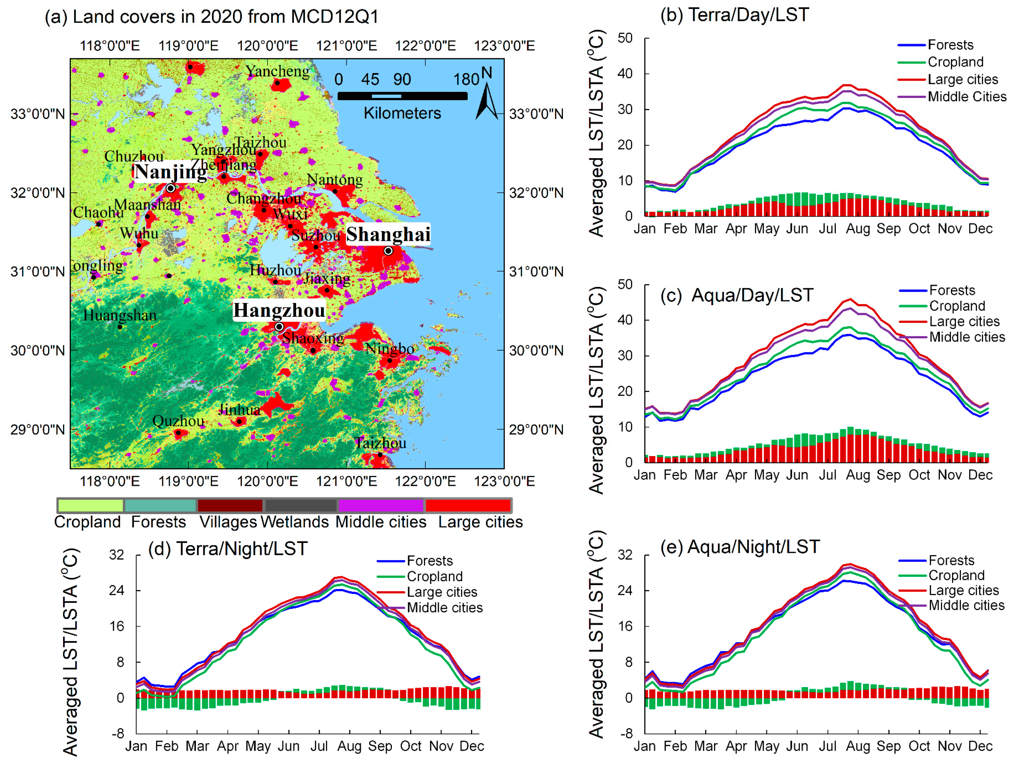
Land cover types mainly consist of cropland, forests, water bodies, and urban and built-up land in the YRDUA region at [117.5–123°E, 28.5–33.7°N] (Figure 1a), with the total area of urban and built-up land of approximately 31,663 km2 in 2020. Spatially continuous large cities with a built-up area exceeding 100 km2 along the Yangtze River and Hangzhou Bay have been identified as representative areas that have notable SUHI effects [4]. These cities are located along the Yangtze River and in Hangzhou Bay and are surrounded by cropland and many medium-size (<100 km2) cities (Figure 1a). Applying the urban population criteria of being more than 1 million, 1 million to 500,000, and below 500,000 from the China Urban Construction Statistical Yearbook [57,58], 15 large, nine medium, and 36 small cities are obtained in the YRD region, with an average built-up area of approximately 414.2, 113.6, and 49.4 km2. Small towns have an average built-up area of approximately 4.6 km2 according to the China Urban–Rural Construction Statistical Yearbook [57,58]. Therefore, large, medium, and small cities and villages are identified from the MCD12Q1 urban and built-up lands by using continuously built-up areas that are ≥ 100 km2, 50–100 km2, 5–50 km2, and <5 km2.
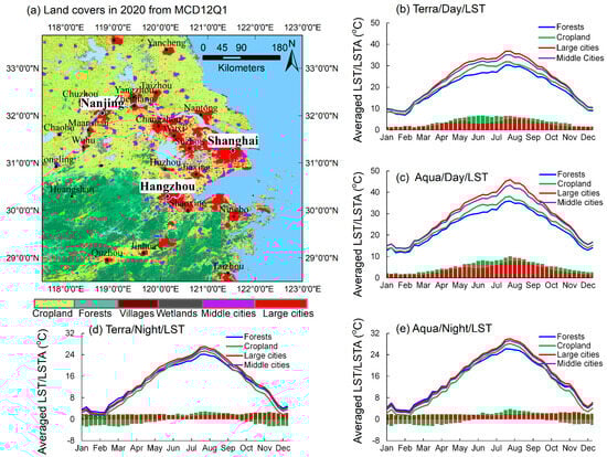
Figure 1.
The MCD12Q1 land cover types in 2020 (a) and long-term mean land surface temperature (LST) annual cycles (lines) during the day and at night for croplands, forests, and medium and large cities, and LST differences between large cities and cropland (red bars), and between cropland and forests (green bars) for Terra (b,d) and Aqua data (c,e) between 2015–2020.
Here, the SUHI zones were defined as areas that have an LST annual cycle similar to that of large cities. Since the Chinese government implemented a development plan to restrict urban expansion in the YRDUA region in 2016, large- and medium-sized cities have maintained a stable urban and built-up area of approximately 7787.6–7818.4 km2 according to the China Urban Construction Statistical Yearbook for 2015–2020 [57,58]. We thus investigated the land thermal features based on differences in the LST annual cycle between medium-sized cities (50–100 km2), large cities, cropland, and forests for the period 2015–2020. Statistically significant differences in the daytime LST annual cycle were found among large cities, medium cities, cropland, and forests in an F-test variance analysis at a 0.01 significance level (lines in Figure 1b,c). There were large LST differences of approximately 4–8 °C between April–September and small differences of less than 2 °C between October–March (red bars in Figure 1b,c). Medium and large cities, cropland, and forests had similar nighttime LST annual cycles, with LST differences of approximately −3 to 3 °C. The daytime LST annual cycle was thus suitable for classifying the land surface thermal zones owing to its statistically significant differences among large cities, medium cities, cropland, and forests.
A spatial similarity regression model (Si) proposed by Xie et al. in 2022 [4] was used to identify areas that have LST annual cycles similar to those of large cities, cropland, and forests. The spatial similarity of the LST annual cycle (Si) to the LST annual cycle of the large cities, cropland, or forests at a grid point was quantified using the explained variance (R2) and the root mean square error (RMSEi), defined as
where Ri is the correlation coefficient, Rmode is the mode of Ri frequencies, Trj is the regionally averaged LST in large cities, cropland, or forests, RMSEi is the root mean square error, is the average value of Trj, Tij and denote the LST series at grid point i and the average value, N is the series length, and and are adjustment factors adopted to avoid the excessive reduction of RMSEi. Si is the spatial similarity of the LST annual cycle to the LST annual cycle of large cities, cropland, or forests at the grid point i, with a statistical confidence level from the chi-square variable . Applying a natural-break algorithm, all Si values were classified into five types that were two zones with strong positive/negative values R~±1.0, two transition zones with positive/negative correlation, and an uncorrelated zone (R~0) by using a natural-break algorithm.
2.4. Estimation of the SUHI Intensity on Each Grid Point in Urban Agglomerations
RF regression is a nonlinear machine-learning technique based on decision trees with good generalization ability, and increasing the critical hyper-parameter ntree can improve the RF model performance and stability [59]. Non-urban LSTs in the background, cropland, and forest zones well-related to the geographical factors, the topographic variables, and biophysical and urbanization parameters, were used to train the RF models adopting the input features listed in Table 1.

Table 1.
Influencing factors of the LST used in random forest models.
Theoretically, there is no need for any additional accuracy estimation procedures like cross-validation or a separate test set to get an estimate of the training error for RF regression owing to the out-of-bag error being estimated internally during the training. Hence, three critical hyper-parameters used in the RF models, the tree depth max_depth, the minimum samples required at a leaf node min_sample_count, and the maximum tree number ntree, were determined by the out-of-bag error at the respective ranges of 5–25, 0.5%–3%, and 5–300 with the increments of 1, 0.1%, and 5 during the training. As a result, all RF models showed a small out-of-bag error of less than 1.0 °C and 1.4 °C at the critical hyper-parameters min_sample_count = 1%, max_depth = 10 and ntree = 200 for the 8-day composite long-term Terra and Aqua LSTs in the period between 2015–2020. The min_sample_count = 1%, max_depth = 10, and ntree = 200 thus were selected as the optimal values. Considering the urban LST background value at each grid point in the SUHI zone as a missing value, these RF models trained by the non-urban LSTs were further used to estimate the urban LST background owing to the advantage of RF regression in estimating a large proportion of missing data with a good accuracy.
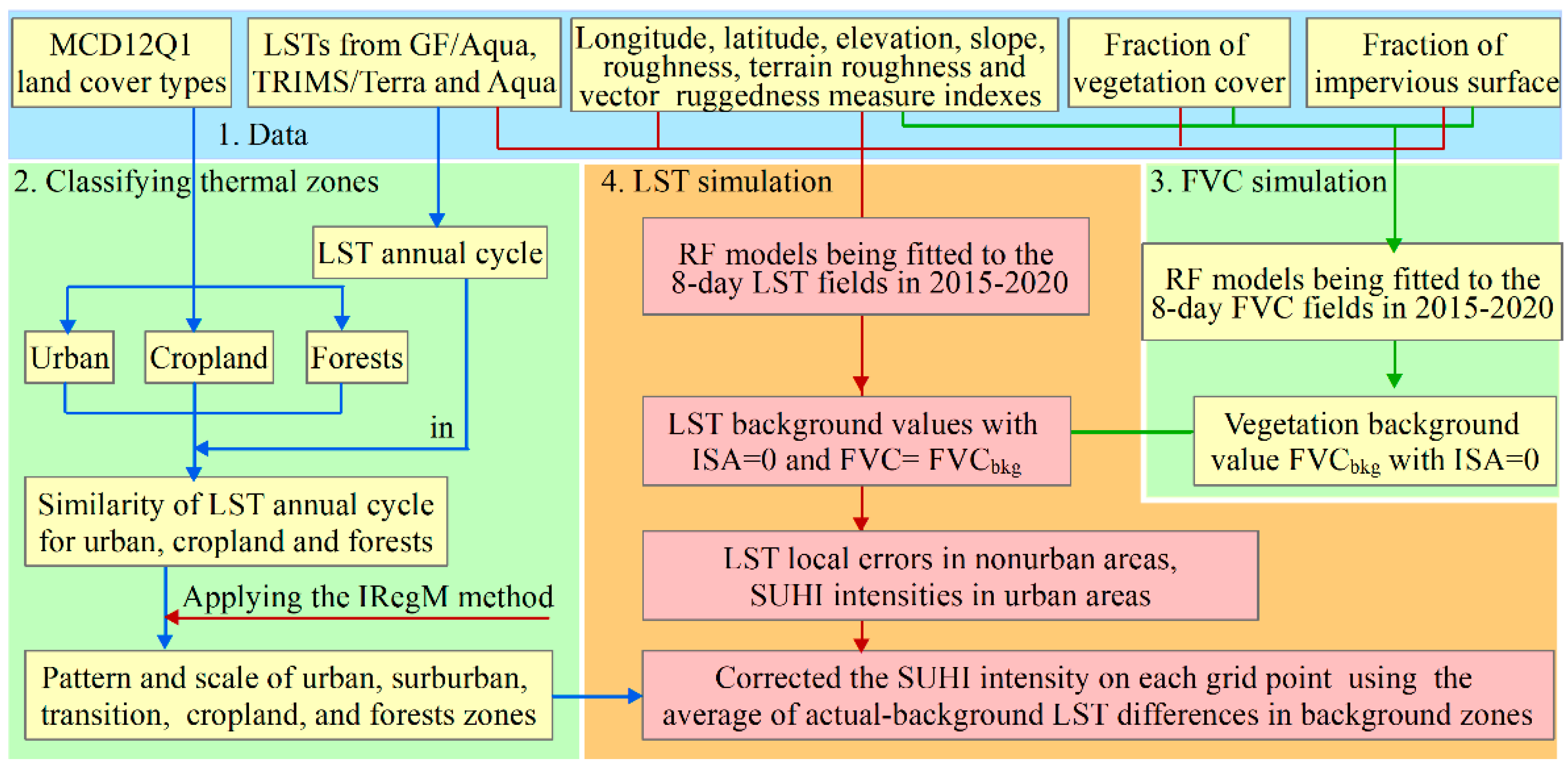
The SUHI intensity at each grid point was estimated by adopting the following procedure. (1) Applying the spatial similarity regression model proposed by Xie et al. (2022) [4], the SUHI zone and its spatial pattern and scale were first identified from the MODIS/LST annual cycle for the YRDUA region between 2015–2020. (2) Strong SUHI zones, vulnerable SUHI zones, background zones, cropland zones, and forest zones were then identified from long-term LST annual cycles similar to those of large cities, cropland, and forests. The LST samples in the background, cropland, and forest zones were used to train RF models. (3) A series of RF models with the hyper-parameters min_sample_count = 1%, max_depth = 10, and ntree = 200 were obtained from each long-term 8-day composite FVC field and non-urban LST field between 2015–2020, and the LST-simulating error was calculated at each grid point. These RF models were further used to estimate the vegetation background FVCbkg with ISA = 0 and the temperature background LSTbkg with ISA = 0 and FVC = FVCbkg at each grid point over strong SUHI zones and the vulnerable SUHI zones. (4) The SUHI intensity was finally obtained from the difference between actual and background LSTs at each grid point over urban agglomerations. The framework is shown in Figure 2.
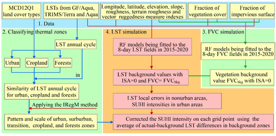
Figure 2.
Framework for characterizing the SUHI spatial pattern and scale and intensity in urban agglomerations.
3. Results
Applying the proposed solution described in Section 2, the strong SUHI zone and the zones being vulnerable to SUHIs were identified out on the similarity of long-term LST annual cycles and successfully excluded the heat islands unrelated to urbanization in the YRDUA region. We also obtained the SUHI intensity, spatial pattern, and scale for each case of the long-term 8-day composite MODIS/LST data between 2015–2020, which were further used to investigate the seasonal variations of the regional SUHIs related to vegetation changes and urbanization. All these are conducive to urban planning and environmental management in terms of shaping rational urban clusters and improving human comfort.
3.1. The SUHI Spatial Pattern and Scale and the Land Surface Thermal Types
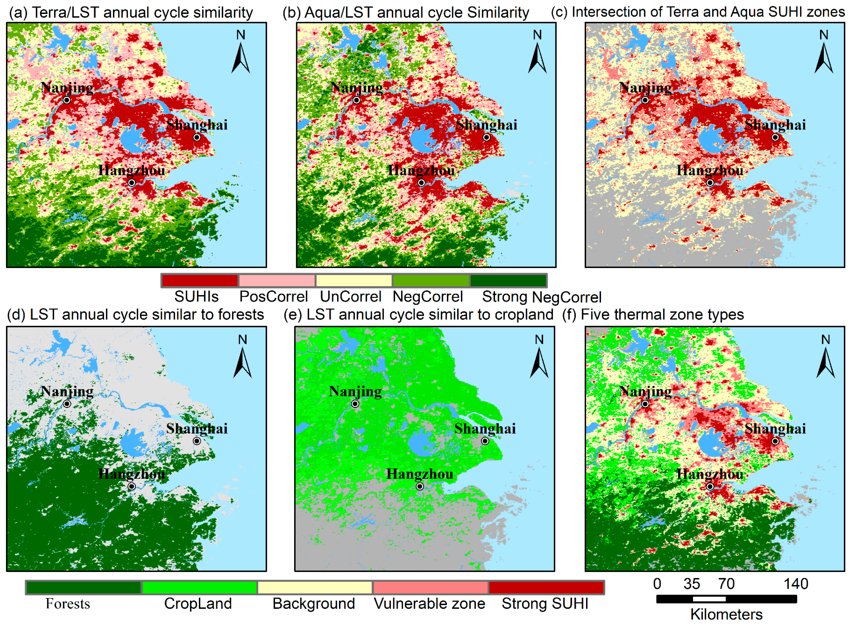
Terra/SUHI and Aqua/SUHI zones were obtained from the spatial similarity of LST annual cycles similar to those in large cities with a chi-square test at 0.05 confidence level, (Figure 3a,b), with the spatial extents of approximately 42,328 km2 and 38,884 km2. Their intersections represented a stable daytime SUHI phenomenon over the middle and large cities (Figure 3c) and were identified as the optimal SUHI zone, with statistical reliability belonging to the SUHIs at each grid point and a spatial scale of approximately 30,636 km2. The thermal zones that have a long-term LST annual cycle similar to that of cropland (forests) were identified from Terra and Aqua satellites, and their union was identified as the cropland (forests) zones (Figure 3d,e). The SUHI zone had notable overlapping areas with cropland and forest zones (Figure 3c–e), which were the mixed areas of built-up land and natural and agricultural vegetation land according to the MCD12Q1 data in 2020. These overlapping areas had an LST annual cycle simultaneously similar to that of large cities, cropland, and forests and were identified as the SUHI vulnerable zone related to urbanization, with a spatial extent of approximately 23,631 km2. A strong SUHI zone was then defined as the difference between the SUHI zone and the SUHI vulnerable zone and had a spatial extent of approximately 7005 km2 compatible with the urban and built-up area of large- and medium-sized cities. Intersections between the cropland and forest zones and the areas uncorrelated with large cities were further defined as background zones without notable UHI effects. Ultimately, the YRDUA region was divided into a strong SUHI zone, vulnerable SUHI zone, background zone, cropland zone, and forest zone (Figure 3f). In summary, the SUHI effects steadily occurred in the strong SUHI zone, they could deteriorate with the urbanization in the vulnerable zone, and they did not occur in the background, cropland, and forest zones. According to the SUHI zone and the urban and built-up land in 2020 MCD12Q1 data, approximately 24,784 km2 of urban and built-up land and 14,098 km2 of non-urban land around large cities showed notable SUHI phenomenon and approximately 6879 km2 of urban and built-up land in small cities and villages that have no SUHI phenomenon. Hence, urban and built-up lands cannot accurately represent the spatial scale and pattern of SUHIs.
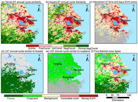
Figure 3.
Strongly positively correlated (also referred to as SUHI), positively correlated, uncorrelated, negatively correlated, and strongly negatively correlated zones that have the Terra/LST (a) and Aqua/LST (b) annual cycles similar to those of large cities and the intersections of Terra/SUHI and Aqua/SUHI zones (c); areas having the LST annual cycle similar to that of forests (d) and the cropland (e); and five thermal zone types (f).
3.2. Estimation of the FVC and LST Backgrounds and the SUHI Intensity
The nonurban LST is well-associated with climate, geographical, topographical, and biophysical conditions, all of which have been well-retrieved from high-quality satellite datasets without gaps or missing values [50,56]. RF regression models were with geographical, biophysical, and urbanization parameters to fit the nonurban LST in the background, cropland, and forest zones and estimate the urban LST background and SUHI intensity at each grid point in the SUHI zone.
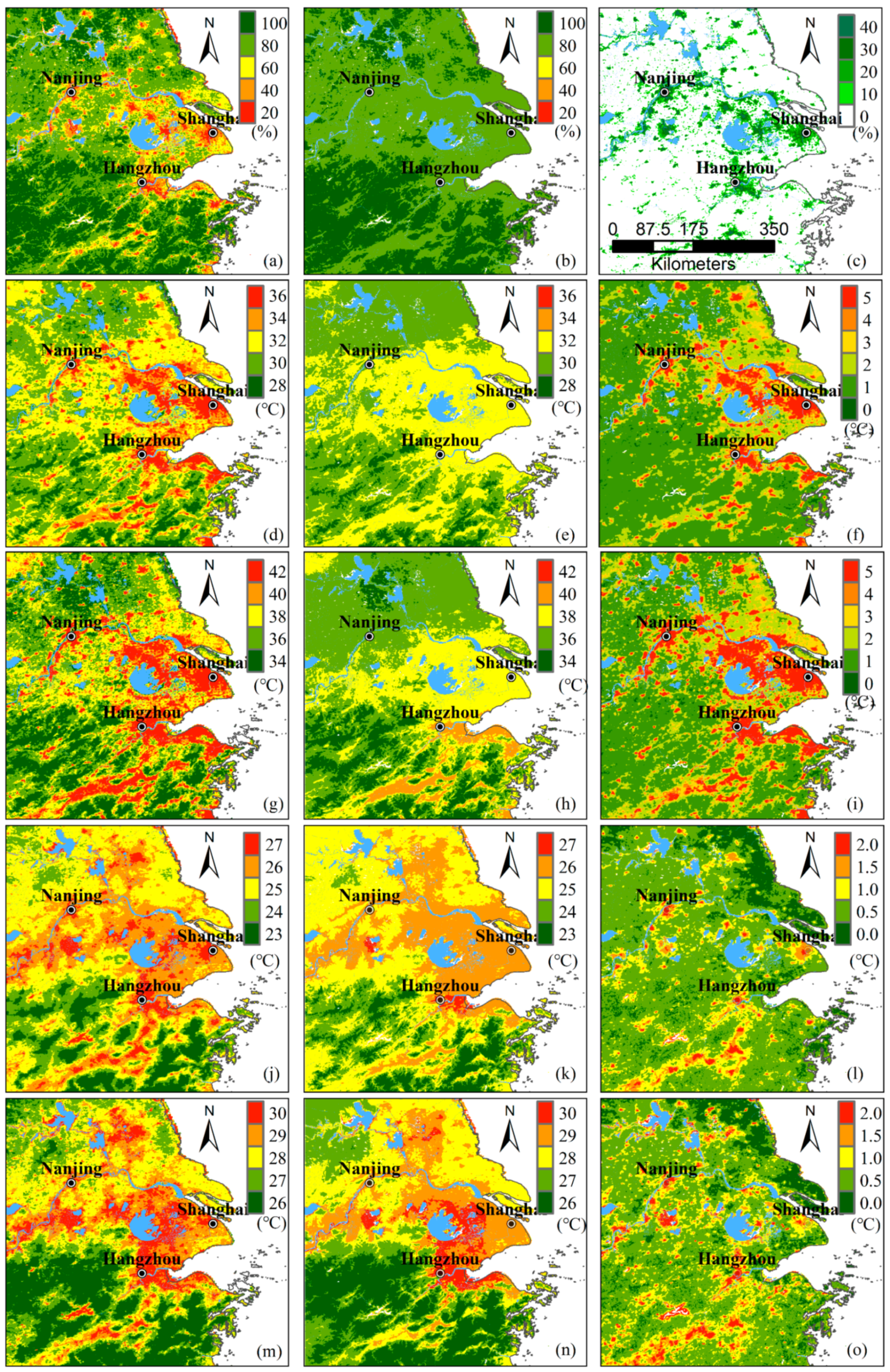
Figure 4 shows an example of estimating the urban FVC and LST backgrounds and quantifying the SUHI intensity on Day 225 of the long-term LST annual cycle between 2015–2020. An RF model was first trained by the FVC samples in the background, cropland, and forest zones with the input features listed in Table 1 at the optimal hyper-parameter ntree = 200 and was used to estimate the vegetation background FVCbkg without the urban effect (ISA = 0) at each grid point in the SUHI zone. In the same way, the LST samples in the background, cropland, and forest zones were used to train another RF model with the input features listed in Table 1 at the optimal hyper-parameter ntree = 200. This RF model was further used to estimate the temperature background LSTbkg with ISA = 0 and FVC = FVCbkg at each grid point in the SUHI zone. As shown in the left and middle panels of Figure 4, the actual FVC and LST values and their estimated backgrounds from the geographical factors, topographic variables, and vegetation background had similar spatial patterns and comparable values in the background, cropland, and forest zones. Almost no urban effects on the FVC and LST backgrounds were observed in the urban areas. Large actual background differences in the FVC and LST (right panel in Figure 4) thus represented urban effects and showed a spatial pattern similar to the urban and built-up land (Figure 1a). The SUHIs reached a maximum intensity of approximately 5 °C during the day and approximately 2 °C at night in the urban areas and valleys of the YRDUA region. Small actual background LST differences below 1 °C were due to RF simulation errors in the cropland and forest zones. Therefore, the RF models simulated the FVC and LST values in the non-SUHI zone well and reasonably estimated the FVC and LST backgrounds in the SUHI zone on Day 225 of the long-term LST annual cycle between 2015–2020.

Figure 4.
Example of estimating the background (middle panel) and the urban effect (right panel) of the fractional vegetation coverage (a–c) and land surface temperature (LST, d–o) on Day 225 of the long-term annual cycle between 2015–2020 using the Random Forest method. Actual value, the RF-estimated background and SUHI intensity for the daytime Terra/LST in (d–f) and Aqua/LST (g–i), and the nighttime Terra/LST (j–l) and Aqua/LST (m–o).
Adopting RF models to fit the nonurban LSTs and estimate the LST background in the SUHI zone for all long-term mean 8-day composite MODIS/LST data between 2015–2020, the results revealed that all RF models performed well in fitting the LSTs in the non-SUHI zone (Figure 5), with the annual MAE value being approximately 0.31 °C for Terra data and 0.44 °C for Aqua data. There were strong seasonal variations of the MAE in the background zones for the daytime LST, with peaks of approximately 0.65 and 0.80 °C for Terra/LST and Aqua/LST data between May–June (Figure 5a,b). The RF models performed well in simulating the LST over background, cropland, and forest zones, with the average MAE being approximately 0.14–0.65, 0.18–0.43, and 0.22–0.38 °C for daytime Terra/LST data and 0.28–0.80, 0.30–0.57, and 0.15–0.50 °C for daytime Aqua/LST data. The cropland and forest zones had a stable MAE of approximately 0.29 and 0.40 °C for the daytime LST of Terra and Aqua data. All RF models simulated the nighttime LST well, with a stable MAE of approximately 0.20–0.30 °C (Figure 5c,d).
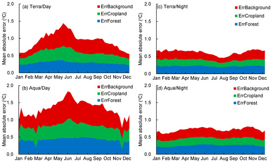
Figure 5.
Seasonal variation of mean absolute errors of the random-forest-estimated land surface temperature (LST) in background, cropland, and forest zones for daytime (a,b) and nighttime (c,d) LSTs from the Terra (a,c) and Aqua (b,d) satellites.
3.3. Seasonal Variations of the SUHI Intensity in the YRDUA Region
As shown in Figure 6, the daytime SUHI intensity in the strong SUHI zone had a strong seasonal variation in the range between 0.93–6.20 °C for Aqua data and 0.29–3.81 °C for Terra data, with an Aqua/SUHI peak in August and two Terra/SUHI peaks of approximately 3.18 and 3.81 °C in May and August (Figure 6a,b). The zone vulnerable to SUHIs had daytime Terra/SUHI and Aqua/SUHI intensities of approximately 0.12–1.85 °C and 0.43–2.74 °C, being half of the intensity in the strong SUHI zone. The strongest daytime SUHI intensity between July–September corresponded to a small RF simulation error of less than 1.0 °C (Figure 5), meaning that the RF models can provide reliable summertime SUHI information for urban planners and decision-makers to design strategies for coping with urban heat waves in the YRDUA region. The cropland zone had a weak cold effect of approximately −1.0 to 0.0 °C for Terra and Aqua data. Nighttime SUHIs had a weak intensity of less than 1.0 °C for Terra and Aqua data (Figure 6c,d).
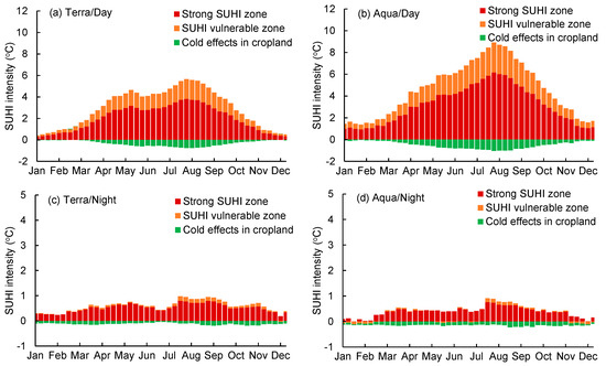
Figure 6.
Seasonal variations of the regionally averaged intensity in the strong SUHI, vulnerable SUHI, and cropland zones from the Terra (a,c) and Aqua (b,d) data.
3.4. Spatial Distribution and Scale of the RF-Estimated SUHI Intensities
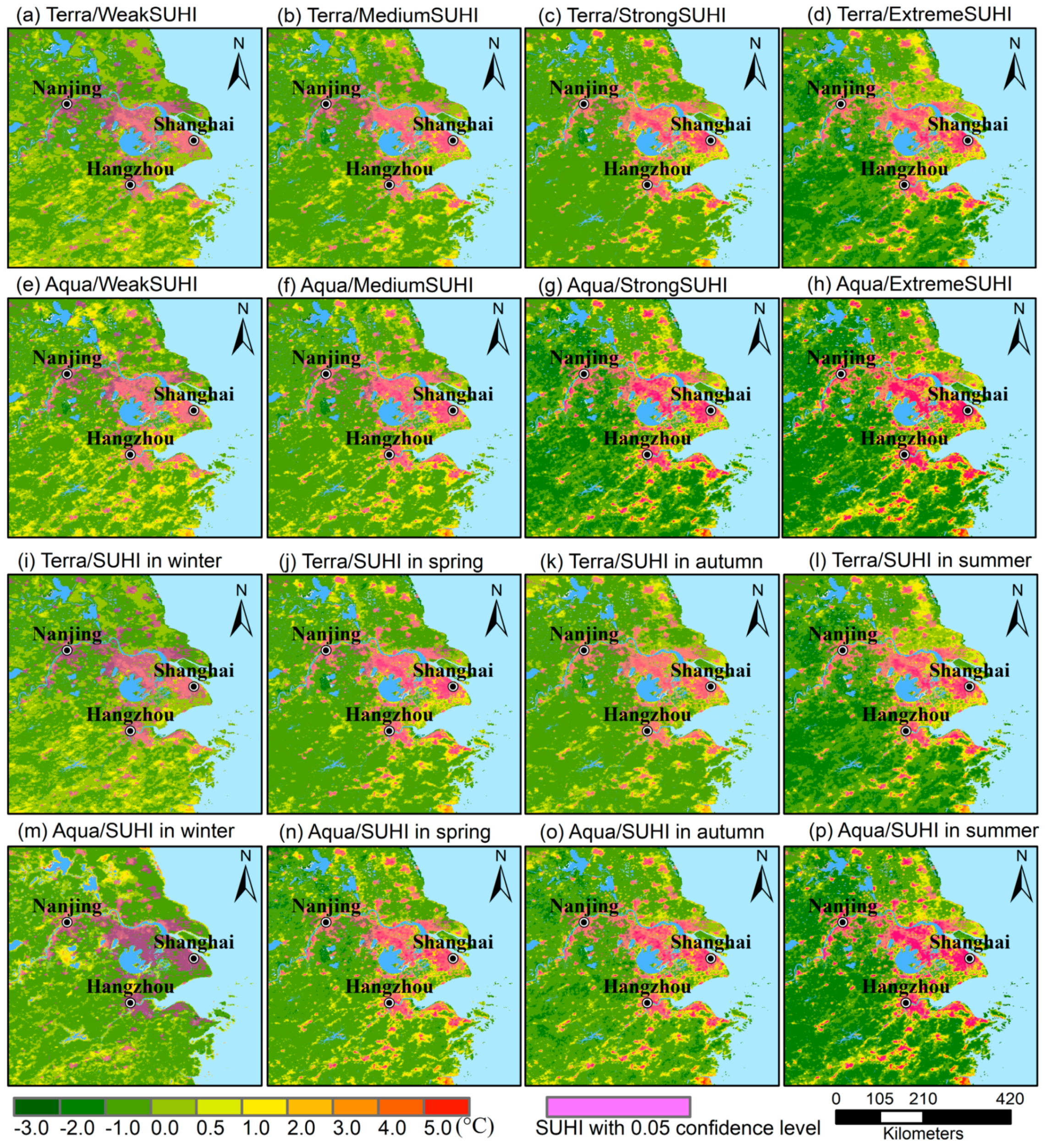
Applying the Jenks–Fisher natural-break algorithm, all daytime SUHIs were divided into weak, medium, strong, and extreme types according to the regionally averaged intensity in the SUHI zones, with the SUHI possessing intensities of 0.18–0.45, 0.46–1.68, and 1.69–2.00 and 2.01–2.59 °C for Terra and 0.60–0.88, 0.89–2.00, 2.01–2.90, and 2.91–4.03 °C for Aqua. The spatial distribution of SUHI intensities of four types is shown in Figure 7a–h. Strong and extreme SUHIs with an intensity of at least 1 °C had spatial extents of approximately 39,528–45,121 km2 for the Terra satellite and 50,078–56,665 km2 for the Aqua satellite, which were larger than the spatial extents of 42,328 km2 and 38,884 km2 obtained from the Terra and Aqua LST annual cycles (Table 2). After the spring sowing of maize, and early harvesting of rice from late July to August over the southern valleys and along the northern coast, some cropland is transformed to bare soil and contributes to the nonurban heat island phenomenon that enhanced the SUHI spatial extent in the strong and extreme types. With the threshold of SUHI intensity increasing from 1.0 °C to 2.0 °C, strong and extreme SUHIs rapidly shrank to the middle and large cities and had the Terra/SUHI and Aqua/SUHI spatial extents of approximately 27,694 km2 and 26,841 km2, which were notably less than those obtained from the Terra and Aqua LST annual cycles. Weak and medium SUHIs had an underestimated extent in the large cities and an overestimated extent in southern YRDUA, with spatial extents of approximately 6612–39,109 km2 and a spatial pattern different from the strong and extreme types. The SUHIs in winter, spring, autumn, and summer showed spatial patterns and variations similar to weak, medium, strong, and extreme types (Figure 7i–p). Therefore, a small amplitude variation in the intensity ranging from 0.5–3.0 °C corresponded to a highly varying spatial extent of the SUHIs among four seasons and the four types of SUHI. The RF models generated more reliable Terra/SUHI and Aqua/SUHI intensities in the extreme type and summer than in other types and seasons owing to the clear urban–rural cliff, low MAE, and statistical reliability at the 0.05 confidence level (purple shading in Figure 7).
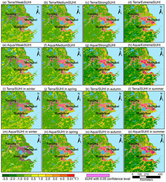
Figure 7.
Spatial pattern and intensity at each grid point for the weak, medium, strong, and extreme SUHI types (a−h) and four seasons (i−p) in the YRDUA region. Green dots represent the grid point identified as the SUHI with a 0.05 confidence level.
Table 2.
The spatial extent of SUHIs at different intensity thresholds.
Table 2 lists the spatial extent of SUHIs for the Terra and Aqua satellites at different intensity thresholds. Compared with the SUHI extents of 42,328 km2 and 38,884 km2 obtained from the Terra and Aqua LST annual cycles, strong and extreme SUHIs had larger spatial extents of approximately 39,528–45,121 km2 for the Terra satellite and 50,078–56,665 km2 for Aqua satellite (Table 2). When the threshold of SUHI intensity varies in the range of 1.0–2.0 °C, strong and extreme SUHIs had smaller spatial extents of approximately 27,694–32,983 km2 for the Terra satellite and 38,798–45,759 km2 for the Aqua satellite. Weak and medium SUHIs had a spatial pattern of approximately 6612–39,109 km2. The SUHIs in winter, spring, autumn, and summer also showed a varying spatial extent at different intensities. In short, it was difficult to identify the reasonable intensity threshold for quantifying the optimal scale and pattern of SUHIs in the YRDUA region. Fortunately, two compatible spatial extents of the SUHI were obtained from the spatial similarity of LST annual cycles similar to those in large cities (Figure 3a,b). Their intersections represented a stable daytime SUHI phenomenon over the middle and large cities and were identified as the optimal SUHI zone of approximately 30,636 km2 for urban design and urban planning.
3.5. Relative Importance of the RF-Model Input Features
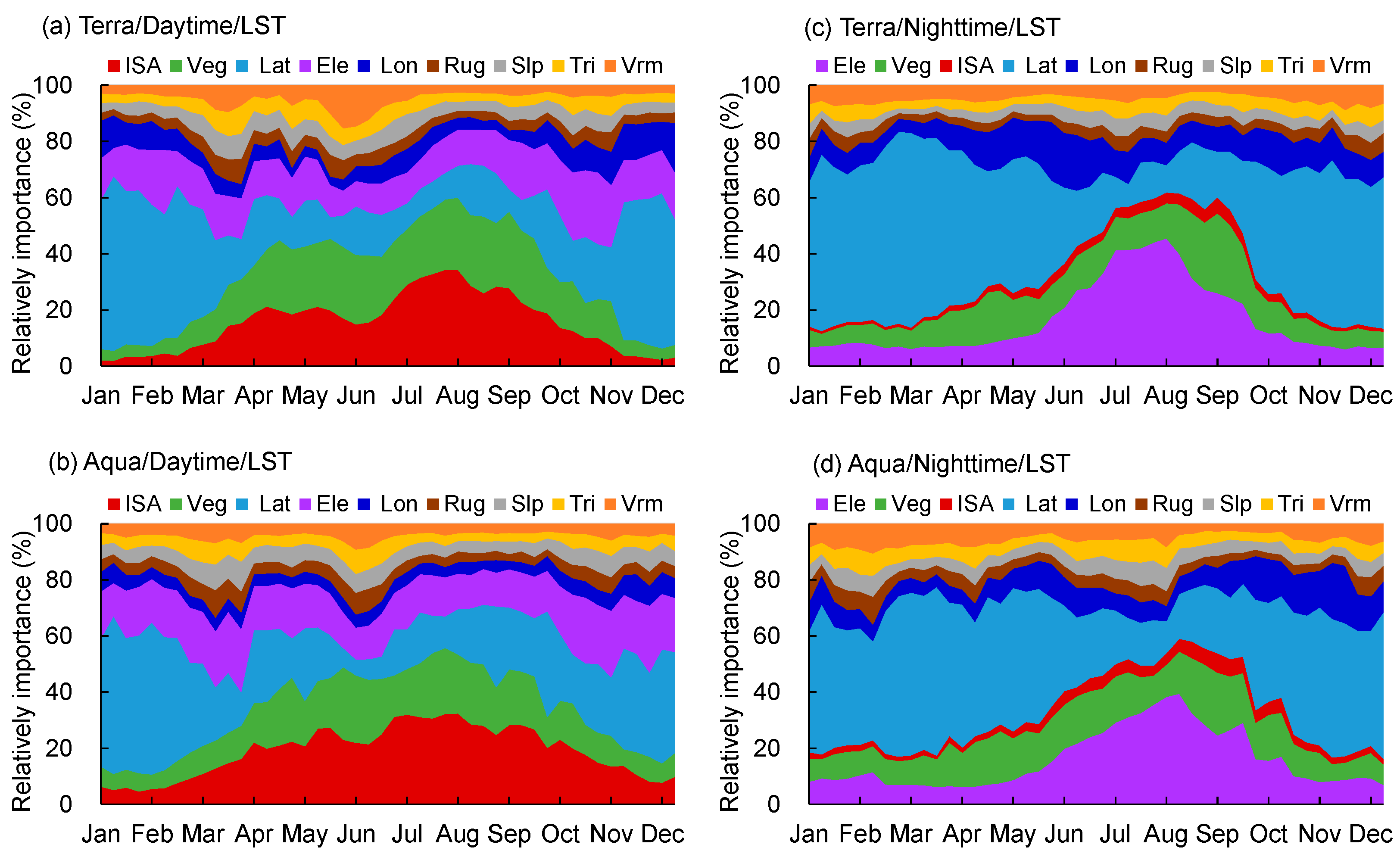
The relative importance values of nine input features were obtained using the RF model regression to fit all actual LSTs in the YRDUA region between 2015–2020. A large importance value means that the feature notably affected the RF model performance in the simulation of the LST spatial distribution and the accuracy of the RF-estimated SUHI intensity. The ISA, FVC, LAT, ELE, and LON features explained approximately 80% of the LST spatial heterogeneity in the YRDUA region (Figure 8a,b). The LAT feature had the largest importance value, exceeding 50%, in the cold season between October–March, and the ISA and FVC features had a large combined importance of approximately 40%–60% and anchored the spatial heterogeneity of the daytime LST in the warm season between April–September. The terrain features of ELE, RUG, SLP, TRI, and VRM, as well as the LON feature, had a stable combined importance of approximately 40% in the daytime LST. In contrast, the ISA and FVC features had small importance values of approximately 15% for the nighttime LST (Figure 8c,d). The topographic variables of RUG, SLP, TRM, and VRM had a combined importance value of less than 20%. The LAT, LON, and ELE features contributed approximately 68% and 63% of the spatial variation of the nighttime Terra/LST and Aqua/LST. The LAT feature contributed more than 50% of the nighttime LST spatial variation between October–May and approximately 20–50% for the Lon feature between June–September. The ISA feature had the lowest importance value of approximately 1–3% in the nighttime LST spatial variation.
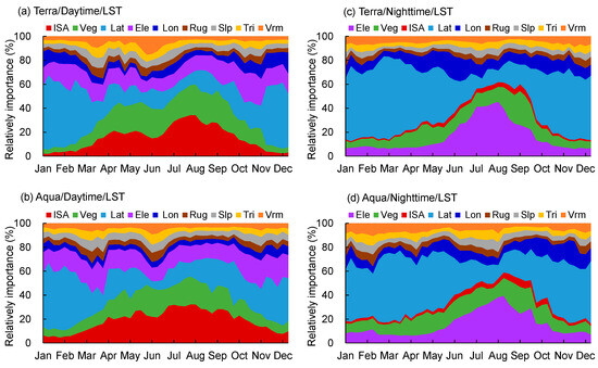
Figure 8.
Seasonal variations in the relative importance of nine inputting features for fitting all actual LST values retrieved from the Terra (a,c) and Aqua (b,d) satellites at day (a,b) and night (c,d) in the YRDUA region.
4. Discussion
4.1. Potential Applications of the Quantitative Regional SUHIs in Urban Planning and Decision-Making
As a phenomenon of any area being warmer than its surroundings, heat islands also can develop in a non-urban area, such as a wetland and water body at nighttime or seasonally bare soil land. These heat islands do not represent a risk to humans or the environment but increase the difficulty of identifying the SUHI spatial pattern and scale and intensity in an urban agglomeration. Anthropogenic heat from vehicles, air-conditioning units, buildings, thermal plants, and other industrial facilities further increase this difficulty [60]. Fortunately, from the perspective of climatology, large cities usually have a daytime LST annual cycle that is statistically significantly different from that of other land cover types at a 0.05 statistical confidence level (Figure 1). Quantifying regional SUHI spatial scales from the spatial similarity of LST annual cycles excluded the heat islands unrelated to the urbanization and captured the SUHI phenomenon extending beyond the urban boundaries over large cities (Figure 2f). Relative to the varying SUHI spatial extents obtained at different intensity thresholds, the statistically reliable spatial pattern and extent identified from the LST annual cycle are more conducive to urban design and planning. The vulnerable SUHI zones that have an LST annual cycle similar to that of large cities, cropland, and forests can provide important references for urban planners and decision-makers in urban design to restrain the rapid expansion of the SUHI spatial extent over urban agglomerations. The strong SUHI zones that have the strongest SUHI intensity and highly urbanized levels should be paid more attention to developing effective mitigation strategies.
Defining the SUHI intensity as the difference between the actual and background LSTs, the non-urban thermal types without SUHI effects: background, cropland, and forest zones that are identified out from the spatial similarity of LST annual cycles at a 0.05 statistical confidence level. The three non-urban thermal types can be used in selecting suitable non-urban LSTs to train the RF models, in which the non-urban LST samples that have notable SUHI effects have been removed to improve the accuracy of estimating the LST background. RF regression can quantify the contribution of various landscape compositions, and biophysical and climate conditions on the LST. Thus, the non-urban LST with the averaged simulation error of approximately 0.31 °C and 0.44 °C is well-fitting for Terra and Aqua satellites, and it reasonably estimated the urban LST background in the YRDUA region. The reliable RF-estimated SUHI intensity in the areas that have an LST annual cycle similar to that of large cities is conducive for urban planners and decision-makers to develop effective mitigation strategies.
4.2. Advantages and Limitations of the Proposed Solution in Quantifying Regional SUHIs
The SUHI spatial heterogeneity in cities cannot be adequately addressed using the traditional urban–rural dichotomy [61]. Defining the SUHI intensity as the difference between the actual and background LSTs, RF regression has clearly shown advantages in estimating the LST background and SUHI intensity at each grid point. It describes the SUHI phenomena based on empirical knowledge and the statistical relationships between LSTs and the geographical, topographic, biophysical, urbanization parameters, and other factors. Although fine-resolution mesoscale simulating models can estimate the LST background and SUHI intensity at each grid point over urban agglomerations, complex data collection, data pre- and post-processing, and model validation make it difficult to simulate complex urbanization processes and human activities over urban agglomerations at a high spatial resolution [27,28]. The two-dimensional Gaussian surface model has been widely used to estimate the SUHI intensity and footprint owing to its good performance in quantifying SUHIs [9,17,30]. Applying a two-dimensional Gaussian surface model to quantify the SUHIs in a single city includes two key steps: First, identifying the rural LST pixels in a single city according to the land cover data. Second, the two-dimensional Gaussian surface models are used to fit the rural LSTs and estimate the urban LST background and SUHI intensity on each grid point in urban areas. Its performance strongly depends on the accuracy of the land cover data and is influenced by the complex terrain and urban geometry. The proposed machine-learning-assisted solution identifies the SUHI zone and rural LST samples from the statistically significant differences in the LST annual cycle between the large cities and other land cover types and reduces the dependence on the land cover data accuracy. More importantly, this solution provides clear urban–rural cliffs and more reliable RF-estimated intensity on each grid point over an agglomeration with a 0.05 statistical confidence level and avoids some heat islands unrelated to urbanization being wrongly marked as SUHIs. Hence, it has great potential in urban planning and design and in mitigating heat-related health risks in rapidly developing urban agglomerations.
Compared with other machine-learning methods [4,7,32], the RF regression avoids the additional accuracy estimation procedures like cross-validation or a separate test set to obtain an estimate of the training error and can quantify the contribution of each inputting feature on the spatial heterogeneity of SUHIs and LSTs over urban agglomerations. The ISA, FVC, LAT, ELE, and LON features explained approximately 80% of the LST spatial heterogeneity in the YRDUA region (Figure 8). The LAT feature had the largest importance value, exceeding 50%, between October–March, and the ISA and FVC features had a large, combined importance of approximately 40–60% and anchored the spatial heterogeneity of the daytime LST between April–September. In contrast, the ISA and FVC features had small importance values of approximately 15% for the nighttime LST, and the LAT, LON, and ELE features contributed approximately 68% and 63% of the spatial variation of the nighttime Terra/LST and Aqua/LST. The main SUHI-related factors are solar radiation, evapotranspiration, land cover type, climate, and geographical factors, topographical and biophysical conditions, and rapid urbanization and other human activities. Most of these factors are well-quantified by high-quality and high-accurate datasets without gaps or missing values [56], and a suite of global 1 km topographic variables has been developed to represent the environmental geographical and topographical conditions [55]. We need to select suitable seasonally varying factors to estimate the urban LST background when quantifying the regional SUHI intensities in urban agglomerations according to the data availability of biophysical parameters for day and night. Among the seasonally varying factors, including the FVC index, normalized difference vegetation index, enhanced vegetation index, leaf area index, surface albedo, downward shortwave radiation, soil moisture, and evapotranspiration, the FVC feature was ultimately identified as the optimal biophysical parameter by adopting RF models owing to its data availability and the ease of estimating the FVC urban background from environmental, geographical, and topographical conditions. The ISA and FVC features represented the effects of urbanization and vegetation relating to solar radiation and biophysical conditions in the YRDUA region.
The proposed solution also has some limitations. A selection of the large cities might strongly affect the accuracy of identifying the SUHI zone and rural LST samples in urban agglomerations, mainly because the SUHI zones are defined as the areas having an LST annual cycle similar to that of the large cities. Spatially continuous large cities with a built-up area of ≥100 km2 have been identified as representative areas that have notable SUHI effects in the YRDUA region. The criterion of built-up areas exceeding 100 km2 for large cities might need further validation before applying it to identify the regional-level SUHIs over other urban agglomerations. Statistically significant differences in the LST annual cycle between large cities and other land cover types are prerequisites for identifying the SUHI zone, but these differences also might not exist in some large cities over arid and desert areas. In addition, the inputting features of RUG, SLP, TRI, VRM, FVC, and ISA for training the RF models usually have a zero value over large lakes, rivers, and large reservoirs, which can lead to the failure of simulating the LSTs over water bodies. In this study, LST samples in large water bodies have been removed from the rural LST samples to generate more accurate RF models in estimating the urban LST background and SUHI intensity (Figure 4 and Figure 7).
5. Conclusions
Since SUHIs have expanded to a regional level and have changed the climate over many urban agglomerations worldwide, mitigating regional SUHIs from the perspective of climatology has become a growing concern for decision-makers and urban planners in terms of actively incorporating UHI-related considerations. Complex urban geometry and human activities, weather and terrain conditions, and some nonurban land being warmer than its surroundings greatly increase the difficulty of characterizing the SUHI intensity, spatial pattern, and scale. Instead of quantifying the complex effects of the urban geometry and human activities on the urban LST, reasonably estimating the urban LST background is a feasible solution for quantifying regional SUHIs in urban agglomerations when defining the SUHI intensity as the difference between the actual and background LSTs. We thus proposed a machine-learning-assisted solution to quantify the SUHI spatial features and intensity at each grid point based on the LST annual cycle in large cities being statistically significantly different from that for other land cover types. This solution provides clear urban–rural cliffs and more reliable RF-estimated intensities of regional SUHIs based on a chi-square testing statistical variable at a 0.05 statistical confidence level and avoids some heat islands unrelated to urbanization being wrongly marked as SUHIs in urban agglomerations. More importantly, we can focus on quantifying the intensity on each grid point without the consideration of the nonurban heat islands when applying machine-learning methods to characterize the SUHIs and the SUHI spatial features that can be reasonably identified from the LST annual cycle over urban agglomerations.
Using the YRDUA as an example and applying the proposed solution, two compatible SUHI spatial scales of approximately 42,328 and 38,884 km2 were obtained from long-term Terra and Aqua LST annual cycles between 2015–2020. The SUHI spatial pattern and scales were identified from the spatial similarity of LST annual cycles at a 0.05 confidence level and excluded the heat island effects of non-urban land such as wetlands, water bodies, and seasonally bare soils. We further adopted an RF method to estimate the urban LST background and SUHI intensity at each 1 km × 1 km grid point using the MODIS-retrieved LST as the response variable and nine satellite-retrieved input variables. By avoiding the quantification of complex effects of the urban morphological factors and human activities on the urban LST, RF models performed well in fitting the nonurban LST values with a low MAE of approximately 0.31 °C for Terra/LST data and 0.44 °C for Aqua/LST data. In addition, the RF models estimated the urban LST background and SUHI intensity in the YRDUA region well. The daytime SUHI intensity in urban zones had a maximum value of approximately 6.20 °C for Aqua/LST data in August and had two peaks of approximately 3.18 and 3.81 °C for Terra/LST data in May and August; these values were approximately 2.2 times the SUHI intensity in suburban zones. The RF models provide more reliable summertime SUHI information in the YRDUA region owing to the low MAE errors of less than 1.0 °C between July–September. This information includes the SUHI spatial pattern and the intensity at each grid point. This feasible solution identifies the strong SUHI and the vulnerable zones and the reliable summertime SUHI intensity on each grid point, all of which are conducive to developing suitable mitigation strategies in different SUHI zones for urban planners and decision-makers. The vulnerable zone, with the SUHI intensity being half of that in the strong SUHI zone, should be paid more attention in urban design to restrain the rapid expansion of the SUHI spatial extent over urban agglomerations.
The reasonable selection of input features in machine-learning methods is critical to quantifying the SUHI intensities in urban agglomerations. SUHI-related factors mainly comprise solar radiation, evapotranspiration, land cover type, climate and geographical factors, topographical and biophysical conditions, and urbanization and human activities. A lack of high-precision and high-resolution climate and weather conditions and human activities could increase the uncertainty in quantifying SUHIs in the YRDUA region. Fortunately, the ISA, VEG, LAT, and ELE explained approximately 80% of the spatial variation of the long-term mean 8-day composite MODIS/LST data between 2015–2020 and anchored the seasonal variation of the daytime SUHIs in the YRDUA region, meaning that it is important to ensure sufficient vegetation to alleviate the SUHIs during rapid urbanization. Our simple solution allows the non-expert to quantify regional SUHIs over urban agglomerations. It is a powerful tool that clarifies urban–rural LST boundaries and provides the reliable land thermal types, the SUHI spatial patterns, and the SUHI intensity on each grid point, and it also indicates the zones that are vulnerable to SUHIs with statistical reliability in urban agglomerations. All these features are conducive to urban planning and environmental management in terms of shaping rational urban clusters, mitigating heat-related health risks, and improving human comfort.
Regional SUHIs gradually extend beyond the urban boundaries in some urban agglomerations and greatly affect the thermal environment of continuous regions and threaten regional-level environmental sustainability, biodiversity, and resource and energy consumption. Machine-learning methods have shown great potential in characterizing the intensity, spatial pattern, and scale of regional SUHIs and their spatiotemporal variations over urban agglomerations. Fine-scale simulation experiments should be conducted simultaneously as a complementary method to machine-learning methods to improve interpretability in future studies, particularly in urban agglomerations that have complex terrain and weather conditions, which could provide more valuable insights for urban design and decision-making.
Author Contributions
Conceptualization, Y.D. and Z.X.; methodology, Z.X.; software, M.W.; validation, N.W. and J.H.; formal analysis, Y.D.; investigation, Y.D. and N.W.; resources, L.Z.; data curation, Y.D.; writing—original draft preparation, Y.D. and Z.X.; writing—review and editing, Z.X.; visualization, N.W. and M.W.; supervision, Z.X.; project administration, Z.X.; funding acquisition, Z.X. All authors have read and agreed to the published version of the manuscript.
Funding
This research was funded by the National Natural Science Foundation of China (Grant 42075118 and Grant 42075027) and the National Key Research and Development Program (Grant 2020YFA0608901).
Data Availability Statement
The daily LST data used in identifying SUHI effects are freely available at the National Tibetan Plateau Data Center (https://doi.org/10.11888/Meteoro.tpdc.271252). The 500 m-resolution yearly land cover type dataset from 2001 to 2020 (MODIS/MCD12Q1) is freely available at https://lpdaac.usgs.gov/products/mcd12q1v061/, accessed on 1 May 2023. The global 30-m-resolution impervious surface dataset with a 5-year interval (1985–2020) is freely available at https://zenodo.org/record/5220816, accessed on 1 May 2023. Data pre- and post-processing and the RF models training are supported by the C/C++ libraries of GDAL at https://gdal.org, accessed on 1 March 2023, Dlib at https://github.com/davisking/dlib, accessed on 1 March 2023, and OpenCV at https://opencv.org/, accessed on 1 March 2023.
Conflicts of Interest
The authors declare no conflicts of interest.
References
- Oke, T.R.; Mills, G.; Christen, A.; Voogt, J.A. Urban Climates; Cambridge University Press: Cambridge, UK, 2017. [Google Scholar] [CrossRef]
- Du, Y.; Xie, Z.Q.; Zeng, Y.; Shi, Y.F.; Wu, J.G. Impact of urban expansion on regional temperature change in the Yangtze River Delta. J. Geogr. Sci. 2007, 17, 387–398. [Google Scholar] [CrossRef]
- Fang, C.; Yu, D. Urban agglomeration: An evolving concept of an emerging phenomenon. Landsc. Urban Plan. 2017, 162, 126–136. [Google Scholar] [CrossRef]
- Xie, Z.Q.; Du, Y.; Miao, Q.; Zhang, L.L.; Wang, N. An approach to characterizing the spatial pattern and scale of regional heat islands over urban agglomerations. Geophys. Res. Lett. 2022, 49, e2022GL099117. [Google Scholar] [CrossRef]
- Manoli, G.; Fatichi, S.; Schläpfer, M.; Yu, K.; Crowther, T. Magnitude of urban heat islands largely explained by climate and population. Nature. 2019, 573, 55–60. [Google Scholar] [CrossRef]
- Masoudi, M.; Tan, P.Y. Multi–year comparison of the effects of spatial pattern of urban green spaces on urban land surface temperature. Landsc. Urban Plan. 2019, 184, 44–58. [Google Scholar] [CrossRef]
- Kim, S.W.; Brown, R.D. Urban heat island (UHI) intensity and magnitude estimations, a systematic literature review. Sci. Total Environ. 2021, 779, 146389. [Google Scholar] [CrossRef] [PubMed]
- Chakraborty, T.; Sarangi, C.; Tripathi, S.N. Understanding diurnality and interseasonality of a sub-tropical urban heat island. Bound.-Layer Meteor. 2017, 163, 287–309. [Google Scholar] [CrossRef]
- Hu, J.; Yang, Y.B.; Zhou, Y.Y.; Zhang, T.; Ma, Z.F.; Meng, X.J. Spatial patterns and temporal variations of footprint and intensity of surface urban heat island in 141 China cities. Sustain. Cities Soc. 2022, 77, 103585. [Google Scholar] [CrossRef]
- Yang, C.B.; Yan, F.Q.; Zhang, S.W. Comparison of land surface and air temperatures for quantifying summer and winter urban heat island in a snow climate city. J. Environ. Manag. 2020, 265, 110563. [Google Scholar] [CrossRef]
- Venter, Z.S.; Chakraborty, T.; Lee, X.H. Crowdsourced air temperatures contrast satellite measures of the urban heat island and its mechanisms. Sci. Adv. 2021, 7, eabb9569. [Google Scholar] [CrossRef]
- Zhang, D.L.; Shou, Y.X.; Dickerson, R.R. Upstream urbanization exacerbates urban heat island effects. Geophys. Res. Lett. 2009, 36, L24401. [Google Scholar] [CrossRef]
- Zhang, N.; Chen, Y. A case study of the upwind urbanization influence on the urban heat island effects along the Suzhou-Wuxi Corridor. J. Appl. Meteorol. Climatol. 2014, 53, 333–345. [Google Scholar] [CrossRef]
- Imhoff, M.L.; Zhang, P.; Wolfe, R.E.; Bounoua, L. Remote sensing of the urban heat island effect across biomes in the continental USA. Remote Sens. Environ. 2010, 114, 504–513. [Google Scholar] [CrossRef]
- Li, X.M.; Asrar, G.R.; Imhoff, M.; Li, X.C. The surface urban heat island response to urban expansion: A panel analysis for the conterminous United States. Sci. Total Environ. 2017, 605, 426–435. [Google Scholar] [CrossRef]
- Zhao, L.; Lee, X.H.; Smith, R.B.; Oleson, K. Strong contributions of local background climate to urban heat islands. Nature 2014, 511, 216–219. [Google Scholar] [CrossRef] [PubMed]
- Zhou, D.C.; Zhao, S.Q.; Zhang, L.X.; Sun, G.; Liu, Y.Q. The footprint of urban heat island effect in China. Sci. Rep. 2015, 5, 11160. [Google Scholar] [CrossRef] [PubMed]
- Sun, Y.W.; Gao, C.; Li, J.L.; Wang, R.; Liu, J. Evaluating urban heat island intensity and its associated determinants of towns and cities continuum in the Yangtze River Delta urban agglomerations. Sustain. Cities Soc. 2019, 50, 101659. [Google Scholar] [CrossRef]
- Wang, Z.A.; Meng, Q.Y.; Allam, M.; Hu, D.; Zhang, L.L.; Menenti, M. Environmental and anthropogenic drivers of surface urban heat island intensity: A case study in the Yangtze River Delta, China. Ecol. Indic. 2021, 128, 107845. [Google Scholar] [CrossRef]
- Zhou, D.C.; Xiao, J.F.; Bonafoni, S.; Berger, C.; Deilami, K.; Zhou, Y.Y.; Frolking, S.; Yao, R.; Qiao, Z.; Sobrino, J.A. Satellite remote sensing of surface urban heat islands: Progress, challenges, and perspectives. Remote Sens. 2019, 11, 48. [Google Scholar] [CrossRef]
- Acosta, M.P.; Vahdatikhaki, F.; Santos, J.; Hammad, A.; Dor′ee, A.G. How to bring UHI to the urban planning table? A data-driven modeling approach. Sustain. Cities Soc. 2021, 71, 102948. [Google Scholar] [CrossRef]
- Chen, S.Z.; Yu, Z.W.; Liu, M.; Da, L.J.; Faiz, M. Trends of the contributions of biophysical (climate) and socioeconomic elements to regional heat islands. Sci. Rep. 2021, 11, 12696. [Google Scholar] [CrossRef] [PubMed]
- Wang, Y.; Li, Y.G.; Xue, Y.; Martilli, A.; Shen, J.; Chan, P.W. City-scale morphological influence on diurnal urban air temperature. Build. Environ. 2020, 169, 106527. [Google Scholar] [CrossRef]
- Back, Y.; Bach, P.M.; Jasper-Tönnies, A.; Rauch, W.; Kleidorfer, M. A rapid fine-scale approach to modeling urban bioclimatic conditions. Sci. Total Environ. 2021, 756, 143732. [Google Scholar] [CrossRef] [PubMed]
- Du, R.; Song, J.; Huang, X.; Wang, Q.; Zhang, C.; Brousse, O.; Chan, P.W. High-resolution regional modeling of urban moisture island: Mechanisms and implications on thermal comfort. Build. Environ. 2022, 207, 108542. [Google Scholar] [CrossRef]
- Zhu, D.; Ooka, R. WRF-based scenario experiment research on urban heat island: A review. Urban Clim. 2023, 49, 101512. [Google Scholar] [CrossRef]
- Feng, Y.; Li, H.; Tong, X.; Chen, L.; Liu, Y. Projection of land surface temperature considering the effects of future land change in the Taihu Lake Basin of China. Glob. Planet Chang. 2018, 167, 24–34. [Google Scholar] [CrossRef]
- Shen, C.H.; Hou, H.; Zheng, Y.Y.; Murayama, Y.J.; Wang, R.C.; Hu, T.G. Prediction of the future urban heat island intensity and distribution based on landscape composition and configuration: A case study in Hangzhou. Sustain. Cities Soc. 2022, 83, 103992. [Google Scholar] [CrossRef]
- Hsu, A.; Sheriff, G.; Chakraborty, T.; Manya, D. Disproportionate exposure to urban heat island intensity across major US cities. Nat. Commun. 2021, 12, 2721. [Google Scholar] [CrossRef]
- Yang, Q.Q.; Huang, X.; Tang, Q.H. The footprint of urban heat island effect in 302 Chinese cities: Temporal trends and associated factors. Sci. Total Environ. 2019, 655, 652–662. [Google Scholar] [CrossRef]
- Yao, L.; Sun, S.; Song, C.X.; Li, J.; Xu, W.T.; Xu, Y. Understanding the spatiotemporal pattern of the urban heat island footprint in the context of urbanization, a case study in Beijing, China. Appl. Geogr. 2021, 133, 102496. [Google Scholar] [CrossRef]
- Adilkhanova, I.; Ngarambe, J.; Yun, G.Y. Recent advances in black box and white-box models for urban heat island prediction: Implications of fusing the two methods. Renew. Sust. Energ. Rev. 2022, 165, 112520. [Google Scholar] [CrossRef]
- Oukawa, G.Y.; Krecl, P.; Targino, A.C. Fine-scale modeling of the urban heat island: A comparison of multiple linear regression and random forest approaches. Sci. Total Environ. 2022, 815, 152836. [Google Scholar] [CrossRef]
- Wang, Q.; Wang, X.N.; Meng, Y.; Zhou, Y.; Wang, H.T. Exploring the impact of urban features on the spatial variation of land surface temperature within the diurnal cycle. Sustain. Cities Soc. 2023, 91, 104432. [Google Scholar] [CrossRef]
- Li, F.; Yigitcanlar, T.; Nepal, M.; Nguyen, K.; Dur, F. Machine learning and remote sensing integration for leveraging urban sustainability: A review and framework. Sustain. Cities Soc. 2023, 96, 104653. [Google Scholar] [CrossRef]
- Lin, J.Y.; Qiu, S.X.; Tan, X.J.; Zhuang, Y.Y. Measuring the relationship between morphological spatial pattern of green space and urban heat island using machine learning methods. Build. Environ. 2023, 228, 109910. [Google Scholar] [CrossRef]
- Du, H.; Wang, D.; Wang, Y.; Zhao, X.; Qin, F.; Jiang, H.; Dai, Y. Influences of land cover types, meteorological conditions, anthropogenic heat and urban area on surface urban heat island in the Yangtze River Delta Urban Agglomeration. Sci. Total Environ. 2016, 571, 461–470. [Google Scholar] [CrossRef]
- Deilami, K.; Kamruzzaman, M.; Liu, Y. Urban heat island effect: A systematic review of spatio-temporal factors, data, methods, and mitigation measures. Int. J. Appl. Earth Obs. Geoinf. 2018, 67, 30–42. [Google Scholar] [CrossRef]
- Peng, J.; Jia, J.; Liu, Y.; Li, H.; Wu, J. Seasonal contrast of the dominant factors for the spatial distribution of land surface temperature in urban areas. Remote Sens. Environ. 2018, 215, 255–267. [Google Scholar] [CrossRef]
- Yu, Z.; Yao, Y.; Yang, G.; Wang, X.; Vejre, H. Spatiotemporal patterns and characteristics of remotely sensed region heat islands during the rapid urbanization (1995–2015) of southern China. Sci. Total Environ. 2019, 674, 242–254. [Google Scholar] [CrossRef] [PubMed]
- Li, Y.F.; Schubert, S.; Kropp, J.P.; Rybski, D. On the influence of density and morphology on the Urban Heat Island intensity. Nat. Commun. 2020, 11, 2647. [Google Scholar] [CrossRef]
- Xiang, Y.; Huang, C.B.; Huang, X.; Zhou, Z.X.; Wang, X.S. Seasonal variations of the dominant factors for spatial heterogeneity and time inconsistency of land surface temperature in an urban agglomeration of central China. Sustain. Cities Soc. 2021, 75, 103285. [Google Scholar] [CrossRef]
- Lau, T.K.; Chen, Y.C.; Lin, T.P. Application of local climate zones combined with machine learning to predict the impact of urban structure patterns on thermal environment. Urban Clim. 2023, 52, 101731. [Google Scholar] [CrossRef]
- Jato-Espino, D.; Manchado, C.; Roldán-Valcarce, A.; Moscardó, V. ArcUHI: A GIS add-in for automated modelling of the Urban Heat Island effect through machine learning. Urban Clim. 2022, 44, 101203. [Google Scholar] [CrossRef]
- Hu, Y.F.; Dai, Z.X.; Guldmann, J.M. Modeling the impact of 2D/3D urban indicators on the urban heat island over different seasons: A boosted regression tree approach. J. Environ. Manag. 2020, 266, 110424. [Google Scholar] [CrossRef]
- Han, D.R.; An, H.M.; Cai, H.Y.; Wang, F.; Xu, X.L.; Qiao, Z.; Jia, K.; Sun, Z.Y.; An, Y. How do 2D/3D urban landscapes impact diurnal land surface temperature: Insights from block scale and machine learning algorithms. Sustain. Cities Soc. 2023, 99, 104933. [Google Scholar] [CrossRef]
- Hou, H.R.; Longyang, Q.Q.; Su, H.B.; Zeng, R.J.; Xu, T.F.; Wang, Z.H. Prioritizing environmental determinants of urban heat islands: A machine learning study for major cities in China. Int. J. Appl. Earth Obs. 2023, 122, 103411. [Google Scholar] [CrossRef]
- Li, L.; Zhan, W.F.; Hu, L.Q.; Chakraborty, T.C.; Wang, Z.H.; Fu, P.; Wang, D.Z.; Liao, W.L.; Huang, F.; Fu, H.Y.; et al. Divergent urbanization-induced impacts on global surface urban heat island trends since 1980s. Remote Sens. Environ. 2023, 295, 113650. [Google Scholar] [CrossRef]
- He, B.J.; Wang, J.S.; Zhu, J.; Qi, J.D. Beating the urban heat: Situation, background, impacts and the way forward in China. Renew. Sust. Energ. Rev. 2022, 161, 112350. [Google Scholar] [CrossRef]
- Tang, W.B.; Zhou, J.; Ma, J.; Wang, Z.W.; Ding, L.R.; Zhang, X.D.; Zhang, X. TRIMS LST: A daily 1 km all-weather land surface temperature dataset for China’s landmass and surrounding areas (2000–2022). Earth Syst. Sci. Data 2024, 16, 387–419. [Google Scholar] [CrossRef]
- Abercrombie, S.P.; Friedl, M.A. Improving the consistency of multitemporal land cover maps using a hidden Markov model. IEEE Trans. Geosci. Remote Sens. 2016, 54, 703–713. [Google Scholar] [CrossRef]
- Yang, L.Q.; Jia, K.; Liang, S.L.; Liu, J.C.; Wang, X.X. Comparison of four machine learning methods for generating the GLASS fractional vegetation cover product from MODIS data. Remote Sens. 2016, 8, 682. [Google Scholar] [CrossRef]
- Gong, P.; Li, X.C.; Zhang, W. 40-Year (1978–2017) human settlement changes in China reflected by impervious surfaces from satellite remote sensing. Sci. Bull. 2019, 64, 756–763. [Google Scholar] [CrossRef]
- Zhang, X.; Liu, L.L.; Zhao, T.T.; Gao, Y.; Chen, X.D.; Mi, J. GISD30: Global 30m impervious-surface dynamic dataset from 1985 to 2020 using time-series Landsat imagery on the Google Earth Engine platform. Earth Syst. Sci. Data 2022, 14, 651–664. [Google Scholar] [CrossRef]
- Amatulli, G.; Domisch, S.; Tuanmu, M.N.; Parmentier, B.; Ranipeta, A.; Malczyk, J.; Jetz, W. A suite of global, cross-scale topographic variables for environmental and biodiversity modeling. Sci. Data 2018, 5, 180040. [Google Scholar] [CrossRef]
- Liang, S.L.; Cheng, J.; Jia, K.; Jiang, B.; Liu, Q.; Xiao, Z.Q.; Yao, Y.J.; Yuan, W.P.; Zhang, X.T.; Zhao, X.; et al. The Global Land Surface Satellite (GLASS) products suite. Bull. Am. Meteorol. Soc. 2021, 102, E323. [Google Scholar] [CrossRef]
- Zhao, H.Z.; Ge, Q.H.; Ni, K. China Urban Construction Statistical Yearbook–2015: National Urban Population and Construction Land by City; China Statistics Press: Beijing, China, 2015; pp. 52–85. [Google Scholar]
- Hu, Z.J.; Wu, W.J.; Xin, Y.N. China Urban Construction Statistical Yearbook–2020: National Urban Population and Construction Land by City; China Statistics Press: Beijing, China, 2021; pp. 48–83. [Google Scholar] [CrossRef]
- Breiman, L. Random forests. Mach. Learn. 2001, 45, 5–32. [Google Scholar] [CrossRef]
- U.S. Environmental Protection Agency. Reducing Urban Heat Islands: Compendium of Strategies. 2008. Available online: https://www.epa.gov/heat-islands/heat-island-compendium (accessed on 20 October 2023).
- Wang, Z.H. Reconceptualizing urban heat island: Beyond the urban-rural dichotomy. Sustain. Cities Soc. 2022, 77, 103581. [Google Scholar] [CrossRef]


Disclaimer/Publisher’s Note: The statements, opinions and data contained in all publications are solely those of the individual author(s) and contributor(s) and not of MDPI and/or the editor(s). MDPI and/or the editor(s) disclaim responsibility for any injury to people or property resulting from any ideas, methods, instructions or products referred to in the content. |
© 2024 by the authors. Licensee MDPI, Basel, Switzerland. This article is an open access article distributed under the terms and conditions of the Creative Commons Attribution (CC BY) license (https://creativecommons.org/licenses/by/4.0/).