Abstract
The height of the F2 peak electron density (hmF2) is an essential parameter in studying ionospheric electrodynamics and high-frequency wireless communication. Based on ionosphere ray propagation theory, the physical relationship between M3000F2 and hmF2 is derived and visualized. Furthermore, based on the above physical theory and the machine learning method, this paper proposes a new model for determining hmF2 using propagation factor at a distance of 3000 km from the ionospheric F2 layer, time, and season. This proposed model is easy to understand and has the characteristics of clear principles, simple structure, and easy application. Furthermore, we used six stations in east Asia to verify this model and compare it with the other three models of the International Reference Ionosphere (IRI) model. The results show that the proposed model (PRO) has minor error and higher accuracy. Specifically the RMSE of the BSE, AMTB, SHU, and the PRO models were 20.35 km, 31.51 km, 13.59 km, and 5.68 km, respectively, and the RRMSE of the BSE, AMTB, SHU, and PRO models were 8.17%, 11.88%, 4.96%, and 2.12%, respectively. In addition, the experimental results show that the PRO model can better predict the trend of the hmF2 inflection point. This method can be further extended to add data sources and provide new ideas for studying the hmF2 over global regions.
1. Introduction
High-frequency (HF) communication is widely applied in various production and daily life domains. For instance, the Global Navigation Satellite System has gained extensive use worldwide through shortwave positioning and communication, particularly in military applications [1]. Because HF communication has the advantages of flexible networking, strong destruction resistance, and high mobility, which can effectively avoid high cost and geographical environment restrictions [2], it is an important research direction [3]. The ionosphere, a variable medium affecting HF communication [4], exhibits time-varying dispersion characteristics. The ionosphere, which includes the thermosphere, part of the mesosphere, and the exosphere, is the ionized part of the upper atmosphere surrounding the earth, extending from 60 km to more than 1000 km [5]. The primary plasma sources are the photoionization of neutral molecules in soft X-ray radiation and the photoionization of neutral molecules in solar EVU [6].
Knowledge of the ionosphere is essential in several applications, such as high-frequency communications, satellite positioning, and navigation systems [7]. The ionosphere consists of the D-layer, E-layer, and F-layer (F1-layer and F2-layer). Among these, the F2 layer exhibits the highest electron density, making it the most significant [8] and stable [9] region in the ionosphere. The height of the peak electron density in the ionospheric F2 layer (hmF2) is one of the critical parameters for predicting the HF communication link [10,11], which represents the distance from the point with the highest electron density in the ionosphere to the ground [12]. The prediction of hmF2 is helpful for the design [13,14] and operation of high-frequency propagation systems [15]. In addition, hmF2 is also helpful for calculating the drift velocity of vertical plasma, studying ionospheric electrodynamics, and enhancing the understanding of space weather environment [16].
Research in this area has been ongoing since the middle of the last century. Shimazaki et al. [17] used Appleton–Beynon data in 1955 to propose an empirical model based on the correlation between hmF2 and the propagation factor at a distance of 3000 km from the F2 layer (identified as M(3000)F2). Later, Bradley and Dudeney [18] improved the above model in 1973 and added correction items. However, this method is impractical in certain cases. In order to solve this problem, Dudeney [19] proposed a new formula based on inverted profiles of high-latitude ionospheric stations in 1975. In 1979, Bilitza et al. [20] proposed a more complex model based on the previous work by using the peak height of the F2 layer measured by incoherent scatter radar, which depended not only on the ratio of foF2 to foE and the number of sunspots but also on the geomagnetic latitude. Finally, this model was included by IRI and became one of the three hmF2 prediction models in IRI. Judging from the above evolution process, the prediction expression of hmF2 has become increasingly complex. However, the study of Adebesin et al. [21] shows that only a simple formula is needed to obtain better prediction results. This model does not directly establish the relationship expression between hmF2 and M(3000)F2, but it uses the solar activity parameter F10.7 to replace M(3000)F2 to develop the relationship expression between hmF2 and F10.7 according to the strong correlation between F10.7 and M(3000)F2 in different seasons and at different times.
Considering the balance of method simplification and precision, this paper proposes a new model between hmF2 and M(3000)F2 according to the season and time (in hours) based on analyzing the strong correlation between hmF2 and M(3000)F2. The structure of this paper is arranged as follows: Section 2 introduces the methodology which includes the physical principle for supporting later modeling, the modeling method, data used for modeling, and the specific modeling process; Section 3 shows experimental results; Section 4 compares the experimental results with the IRI model. In the end, a conclusion is given.
2. Methodology
2.1. Physical Principle
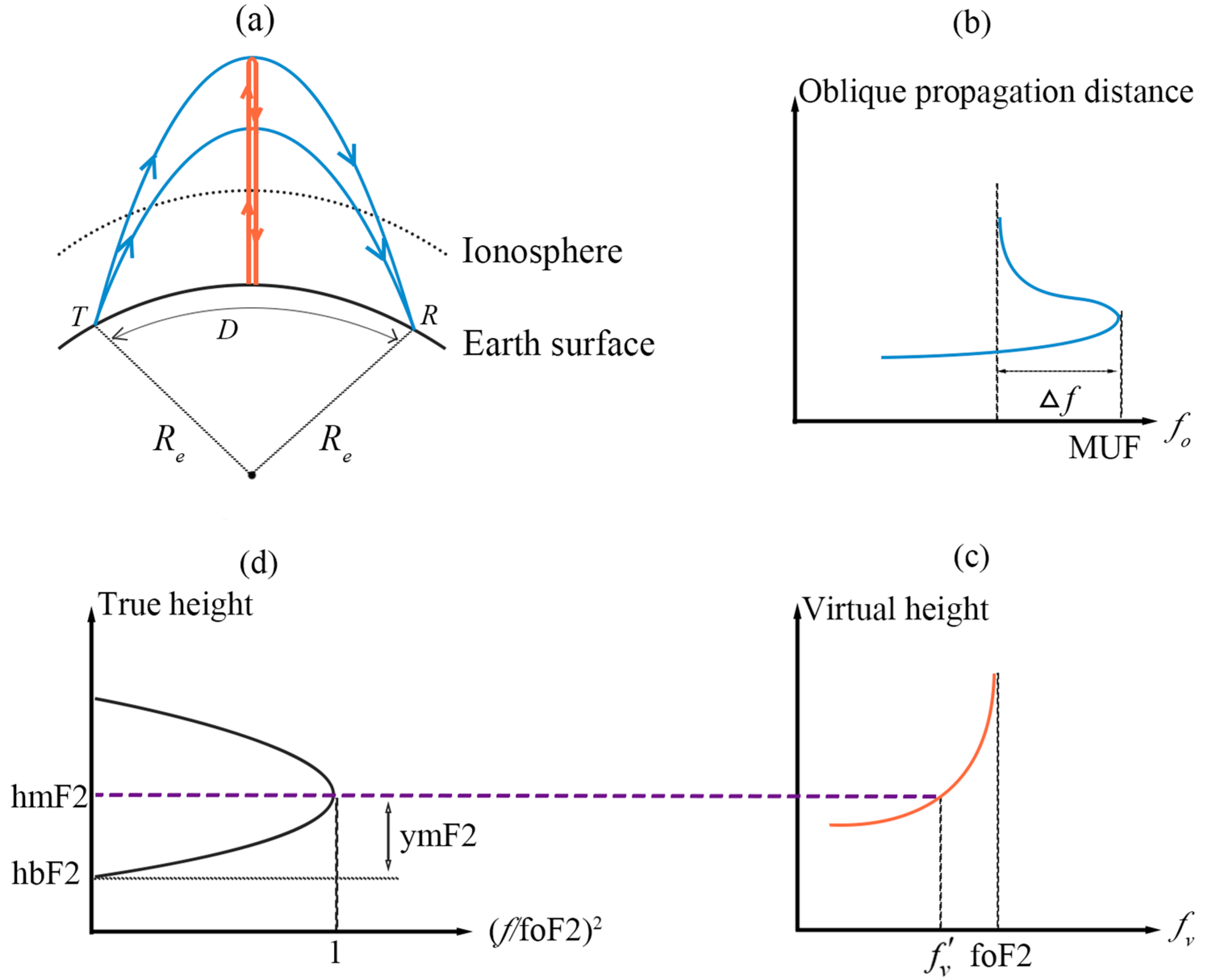
As shown in Figure 1a, ionospheric vertical sounding means that the transmitting position (T) and the receiving position (R) are located at the same position. In contrast, the T and R are located at different positions during oblique ionospheric sounding. Figure 1b shows the curve of virtual height against oblique sounding frequency, and Figure 1c shows the curve of traveling time delay and vertical sounding frequency.
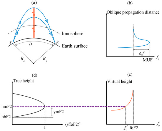
Figure 1.
The relationship between vertical and oblique sounding in the ionospheric F2 layer: (a) Wave transmission path of vertical and oblique sounding; (b) Oblique propagation distance–frequency curve of oblique sounding; (c) Virtual height–frequency curve of vertical sounding; (d) Parabolic distribution of the electron density.
In the following analysis, we ignore the influence of the geomagnetic field and assume that the electron density distribution is parabolic (Figure 1d). For ordinary waves, the relationship between the vertical sounding frequency fv′ corresponding to the peak height hmF2 and the critical frequency foF2 of the F2 layer is as follows [17]:
According to the ray propagation theory [4], the oblique propagation frequency fo corresponding to fv can be expressed as [17]:
where MUF is the maximum usable frequency, M is the propagation factor, Δf is the deviation from MUF, and δ is the rate deviation from MUF.
According to Figure 1a,d, the hmF2 can be represented as
where Re is the radius of the Earth, and its value is 6370; D is the propagation distance between T and R; ymF2 is the half thickness of the ionospheric F2 layer; and hbF2 is the bottom height of the ionospheric F2 Layer. When D is 3000 km, then M is M(3000)F2, and the following results can be obtained:
where hbF2 = hmF2 − ymF2.
In conclusion, hmF2 is a function related to M(3000)F2, ymF2, and δ.
In actual observation, the above parameters vary within a specific range [17]. Suppose that M(3000)F2 varies from 2.5 MHz to 4 MHz, ymF2 varies from 60 km to 120 km, and δ varies from −0.07 to −0.04. The relationship between hmF2 and the above three variables is shown as follows:
As shown in Figure 2, when ymF2 and δ are constant, hmF2 and 1/M(3000)F2 are always approximately linear, so Equation (4) can be simplified as follows:
where C0 and C1 are variables related to ionospheric parameters; however, the ionosphere varies with time, season, and latitude [22,23]. Shimazaki [17] pointed out in his experiment in 1955 that the diurnal variation of hmF2 in the middle and high latitudes has seasonal characteristics, and there are apparent semi-diurnal variations in the middle and low latitudes. According to the above characteristics, this paper intends to train the hmF2 prediction model for different seasons and days, namely Equation (6).
where s is the factor related to the season, and t is the factor related to the daily variation (i.e., the hour).
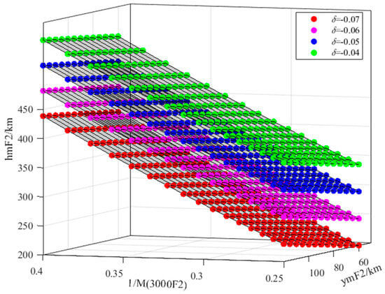
Figure 2.
Relationship between hmF2 and M(3000)F2, ymF2, and δ: the four planes from bottom to top correspond with δ = −0.07, −0.06, −0.05, and −0.04, respectively. Since the differences in hmF2 between the four conditions were particularly small, in order to show them clearly, the hmF2 value with δ = −0.06, −0.05, and −0.04 has been increased by 50, 100, and 150 km, respectively.
2.2. Modeling Method
In this paper, we used statistical machine learning (SML) methods to determine the hyperparameters (C0(s,t) and C1(s,t)) in Equation (6). SML is a multidisciplinary specialty including the knowledge of statistics, probability theory, and complex algorithms. SML is a research hotspot and an important branch of artificial intelligence [24]. Traditional statistics is more inclined toward pure mathematics or theory. However, SML is more inclined toward the intersection of mathematics and computers, and statistical theories often need to be transformed into practical algorithms through learning research. SML uses data and statistical methods to improve system performance. Compared with black box operations such as artificial neural networks, SML has more advantages, such as that its model parameters are often more interpretable and easier to understand [2].
SML is a tool that simulates the human learning process and builds algorithm mappings between inputs and outputs to improve the performance of specific algorithms [20]. SML needs to address four questions [25]: What data need to be selected? How should we select the model, determine the model, and evaluate the model? This corresponds to the three elements of statistical machine learning [25]: model, algorithm, and strategy.
- (1)
- Data are the core of SML, which should have certain statistical regularity and be similar data with some common properties.
- (2)
- The model of SML can be understood as a function, that is, to find the relationship between the input and output variables. Through previous analysis, it has been determined that the relationship between hmF2 and 1/M3000F2 is approximately linear (Equation (6)). M(3000)F2 is the input variable, and hmF2 is the output variable. C0(s,t) and C1(s,t) are the intercept and slope of the model, respectively, which are unknown quantities in the model. It needs to be determined by selecting a suitable algorithm.
- (3)
- SML primarily uses supervised learning to determine the model, and the task of supervised learning is to obtain the mapping relationship between input and output through learning. Specifically, the specific values of hyperparameters C0(s,t) and C1(s,t) in Equation (6) need to be determined through supervised learning. Considering that the model can be reduced to a linear function of one variable, the least squares (LS) regression analysis method is chosen in this paper to find the best function matching of the data by obtaining the sum of squares that minimizes the error.
- (4)
- SML needs to set model evaluation criteria to evaluate the merits and demerits of the trained model, in which root mean square error (RMSE) and relative root mean square error (RRMSE) are selected. RMSE can evaluate performance changes and characterize the impact caused by data perturbations, while RRMSE is used to assess the percentage of relative performance changes [26].
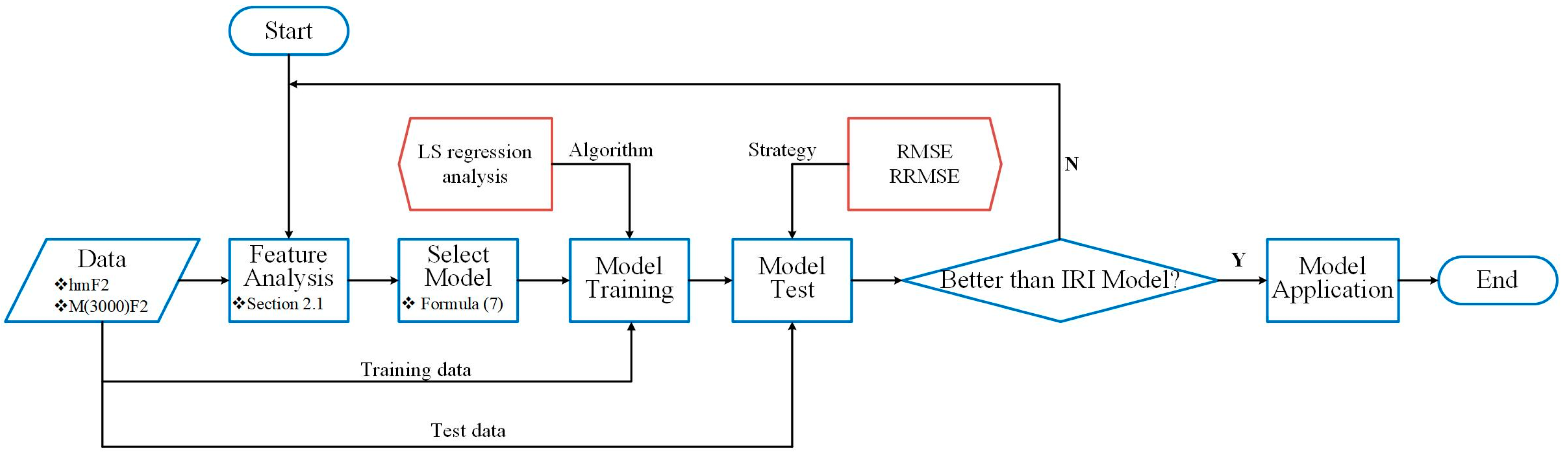
As illustrated in Figure 3, we used the LS regression analysis to determine the model based on the linear relationship between hmF2 and 1/M(3000)F2, and RMSE and RRMSE were chosen as evaluation metrics to assess the performance of this model compared to the IRI model.

Figure 3.
Schematic diagram depicting the experimental procedure based on the SML method.
2.3. Data Collecting
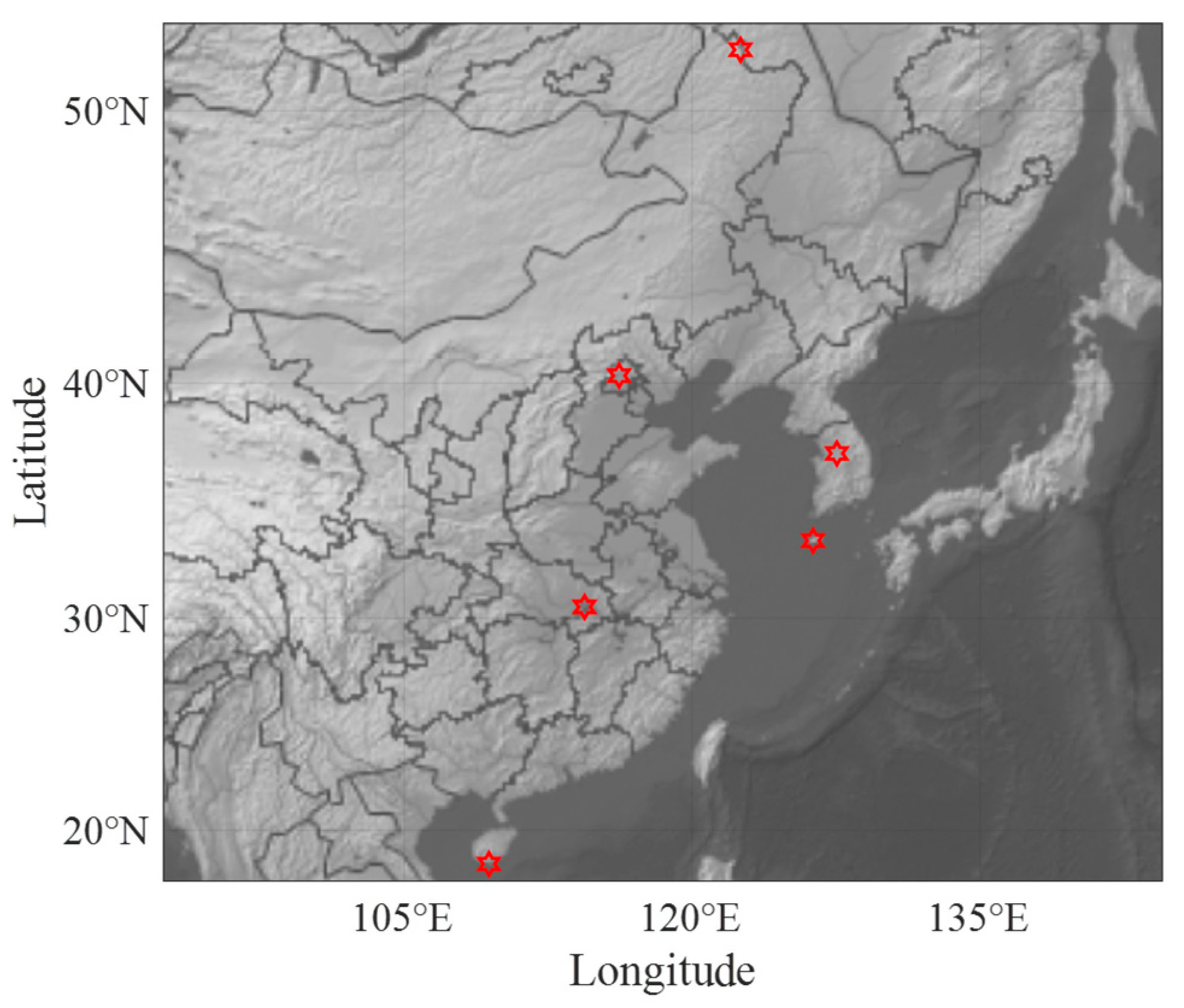
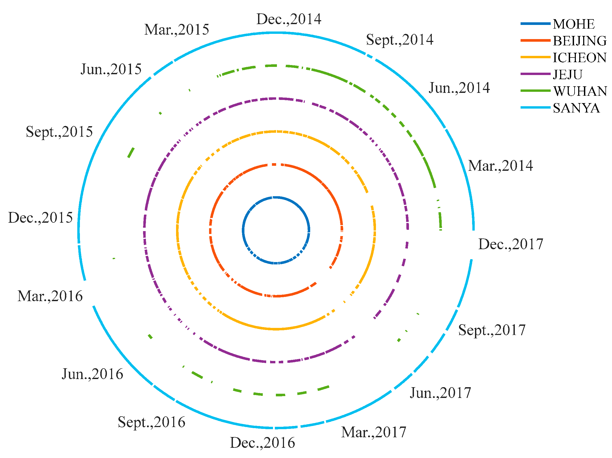
We downloaded the ionospheric data (hmF2 and M(3000)F2) from https://giro.uml.edu/didbase/scaled.php (accessed on 1 May 2023), which was obtained by the Ionosonde. We selected six stations in east Asia, covering middle and low latitudes. Specifically, we selected four stations in China (Mohe, Beijing, Wuhan, and Sanya) and two stations in South Korea (Icheon and Jeju). In addition to the Sanya station located in the low-latitude area, all other stations are located in the mid-latitude area. The geographic locations marked with red hexagrams in Figure 4 are the locations of the six stations used in this paper. hmF2 and M(3000)F2 use the median value, which is the corresponding median value under each hour of each month. Figure 5 shows the training data used in this paper, including the station’s name used for modeling and the time information. The circle in the figure represents the time from 2014 to 2017. The curve indicates that hmF2 and M(3000)F2 are recorded simultaneously at the corresponding time. The station names corresponding to the different colored line segments are in the upper right corner.
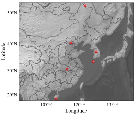
Figure 4.
Latitude and longitude information from the six stations. From top to bottom in turn: Mohe, Beijing, Icheon, Jeju, Wuhan, and Sanya.
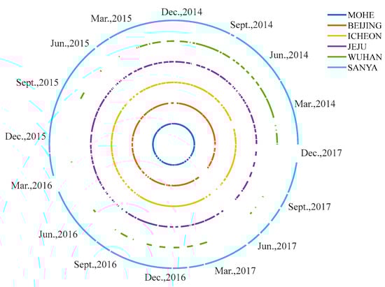
Figure 5.
Training data information.
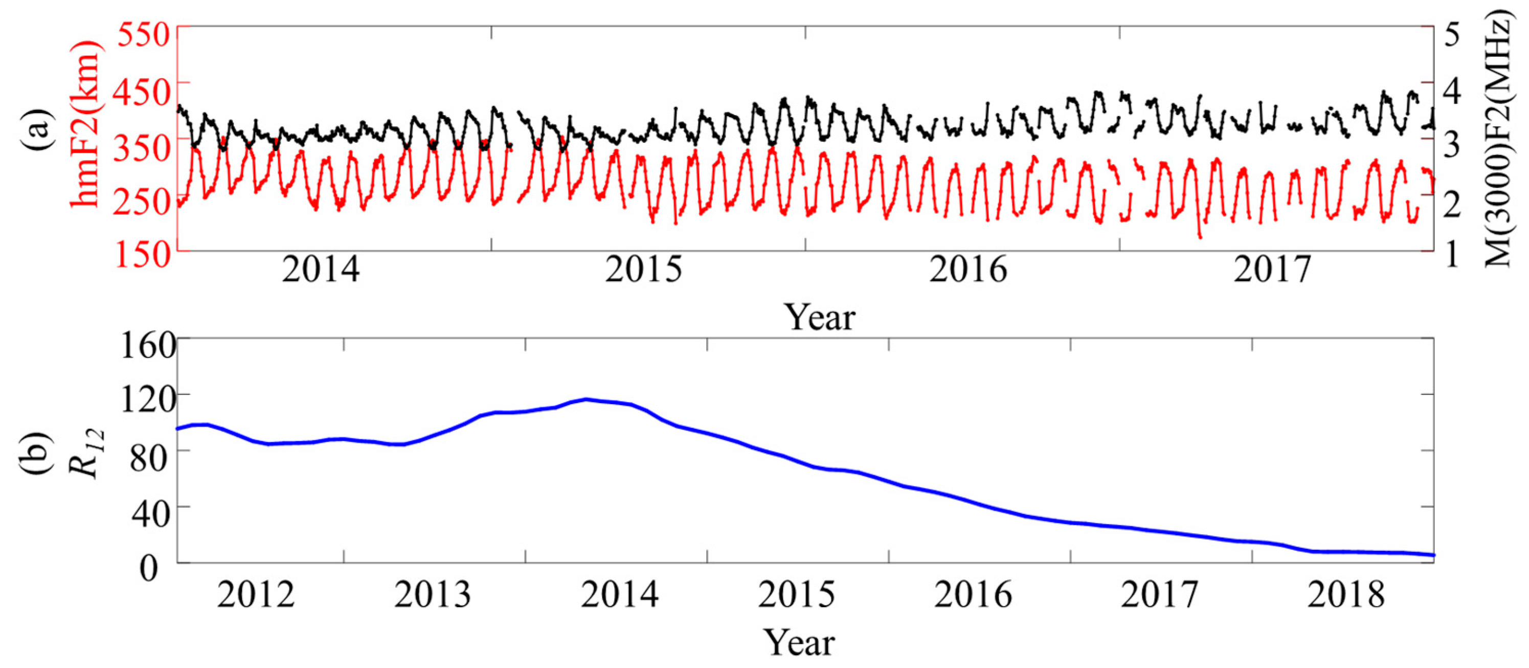
Table 1 shows the detailed information of the verification data used in this paper, and it distinguishes solar activity periods according to Figure 6b. Figure 6a draws the measured data of hmF2 and M(3000)F2 at the Mohe station from 2014 to 2017. The red line represents hmF2, and the black line represents M(3000)F2. There is a negative correlation between the hmF2 and M(3000)F2. In other words, there is a positive correlation between hmF2 and 1/M(3000)F2. Figure 6b plots the twelve-month smoothed value of sunspots from 2012 to 2018, and these values can be obtained from https://www.sidc.be/silso/datafiles (accessed 28 October 2022). We know that, in the period from 2014 to 2017, there was a decline in solar activity. The years 2012 and 2013 were high solar activity years, and 2018 was a low solar activity year.

Table 1.
Validation data information.
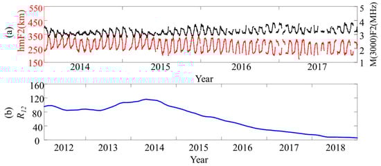
Figure 6.
(a) Measured data of hmF2 and M(3000)F2 at Mohe station from 2014 to 2017; (b) The twelve-month smoothed value of sunspots from 2012 to 2018.
2.4. Modeling Process
Previous analyses have shown that hmF2 is a linear function of 1/M(3000)F2 and is related to seasonal and diurnal variations. According to Lloyd’s season division method [27], seasons are divided into equinox, summer, and winter. According to the different seasons and hours, the corresponding model expression is preliminarily established as shown in (7), where C0(s,t) is the intercept, C1(s,t) is the slope of hmF2 and 1/M(3000)F2, t is the time-dependent factor, and s is the Lloyd season-dependent factor. The division of seasonal factors originated from Lloyd’s harmonic analysis of monthly observations of diurnal variations in the geomagnetic field in Dublin, where similar results were observed in the autumn and spring months [28]. Lloyd’s season divides the 12 months into 3 seasons of 4 months each. In the northern hemisphere, the equinoxes are in March, April, September, and October; summer is May to August, and winter is November to February.
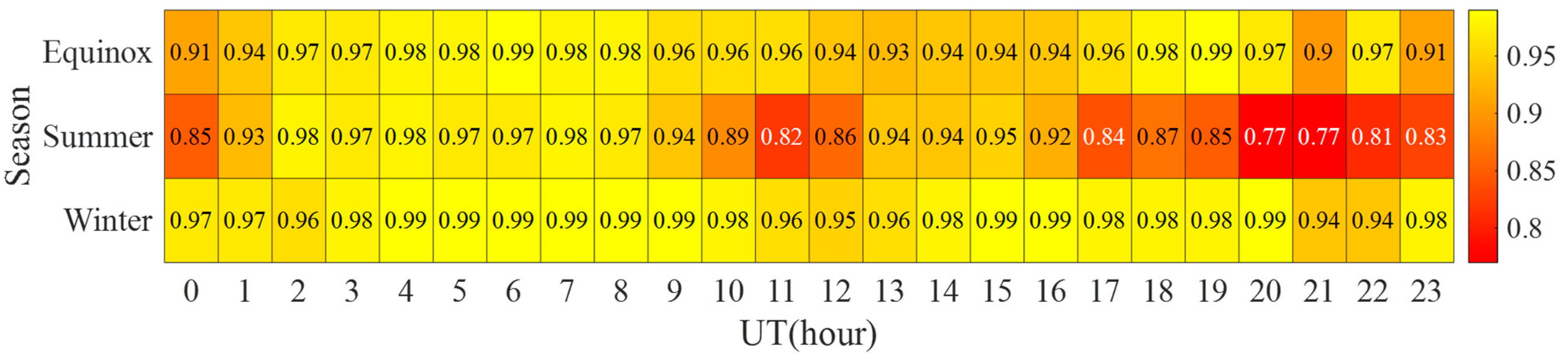
In order to measure the close relationship between hmF2 and 1/M(3000)F2, we first calculated the correlation between hmF2 and 1/M(3000)F2 according to season and universal hour (UT). The calculated results are shown in Figure 7. The correlation between equinox and winter is high, greater than or equal to 0.9, while the correlation between summer and autumn is relatively low. However, except for the correlation between UT = 20 and UT = 21, which is 0.77 and less than 0.80, the correlation between the remaining times is more significant than 0.8, which also provides the possibility for predicting hmF2 by 1/M(3000)F2.
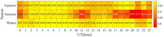
Figure 7.
Correlation between hmF2 and 1/M(3000)F2 of six stations.
Therefore, the training is conducted through (6), where the coefficients C0(s,t) and C1(s,t) are determined by the LS regression analysis method, that is, a group of C0(s,t) and C1(s,t) are found to minimize the sum of squares of the deviation between the predicted value of the model and the actual value, as shown in (7):
where C0(s,t) + C1(s,t)/M(3000)F2n is the predicted value, and hmF2n is the measured value.
Then, the trained model is evaluated, and the evaluation index is RMSE and RRMSE as follows:
where is the predicted value, hmF2n is the measured value, N is the actual data quantity, and n is an integer from 1 to N. If the subscript n differs, the corresponding parameter values are also different.
3. Results
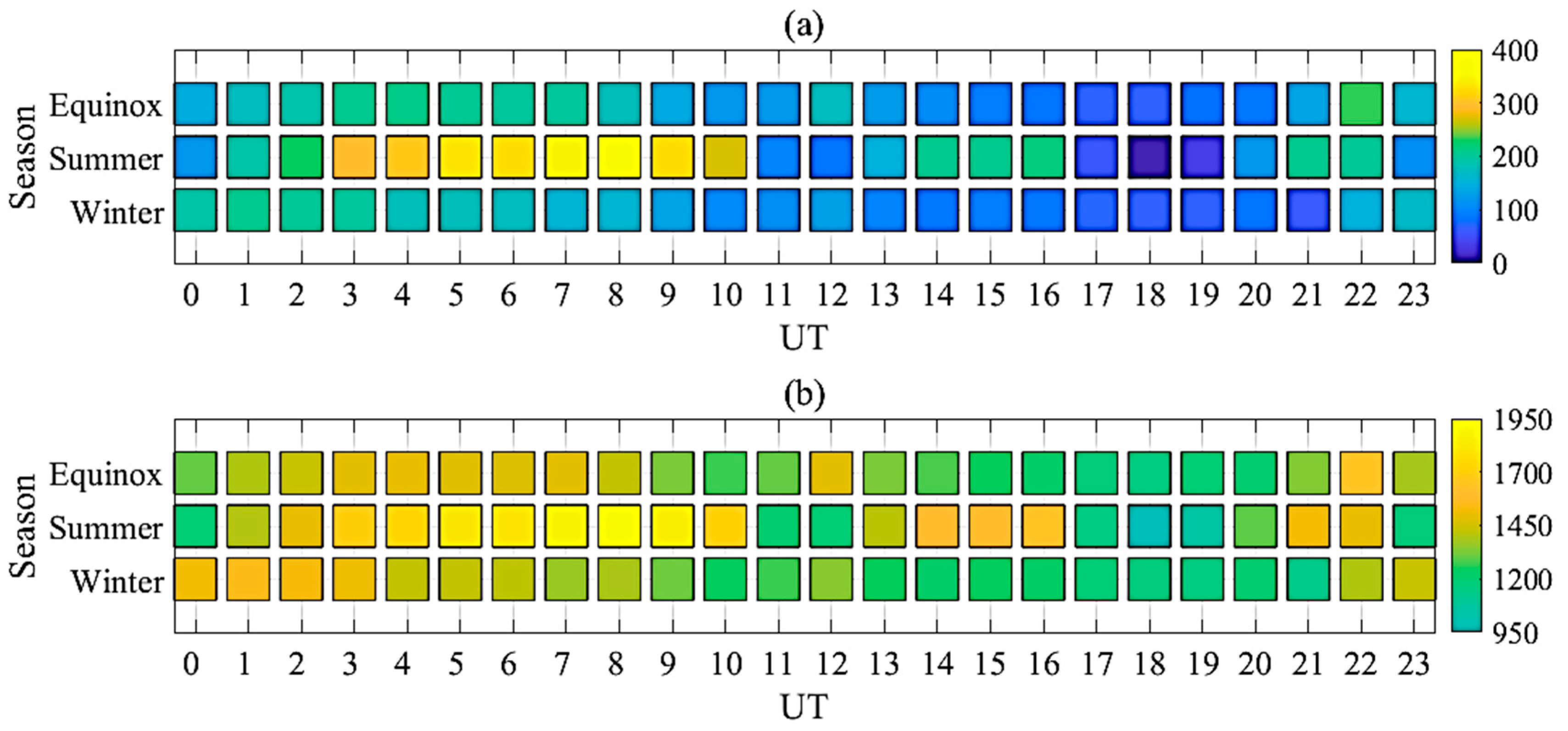
Observed data from 2014 to 2017 were trained according to season and UT, and the corresponding C0(s,t) and C1(s,t) were obtained. Figure 8a shows the inversion value of C0 at different UTs in different seasons, which is similar to C1(s,t). When UT = 8 in summer, C0(s,t) has the maximum value of 3.5524 × 10²; when UT = 18 in summer, C0(s,t) has the minimum value of 3.257. Figure 8b shows the value of C1(s,t) in different seasons and at different UTs. When UT = 8 in summer, C1(s,t) has a maximum value of 1.9255 × 10³; when UT = 18 in summer, C1(s,t) has a minimum value of 9.742 × 10².
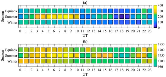
Figure 8.
The values of C0 and C1 obtained by training in different seasons and universal time: (a) C0; (b) C1.
In order to measure the fitting degree of the model to the observed value, the respective goodness of fit (defined as R2) is calculated according to season and universal time, respectively. Namely,
where is the predicted value, is the average of the measured value, N is the actual data quantity, and n is an integer from 1 to N. If the subscript n differs, the corresponding parameter values are also different.
The value of the goodness of fit R2 ranges from 0 to 1. The closer the value is to 1, the better the degree of fit; the closer the value is to 0, the worse the degree of fit.
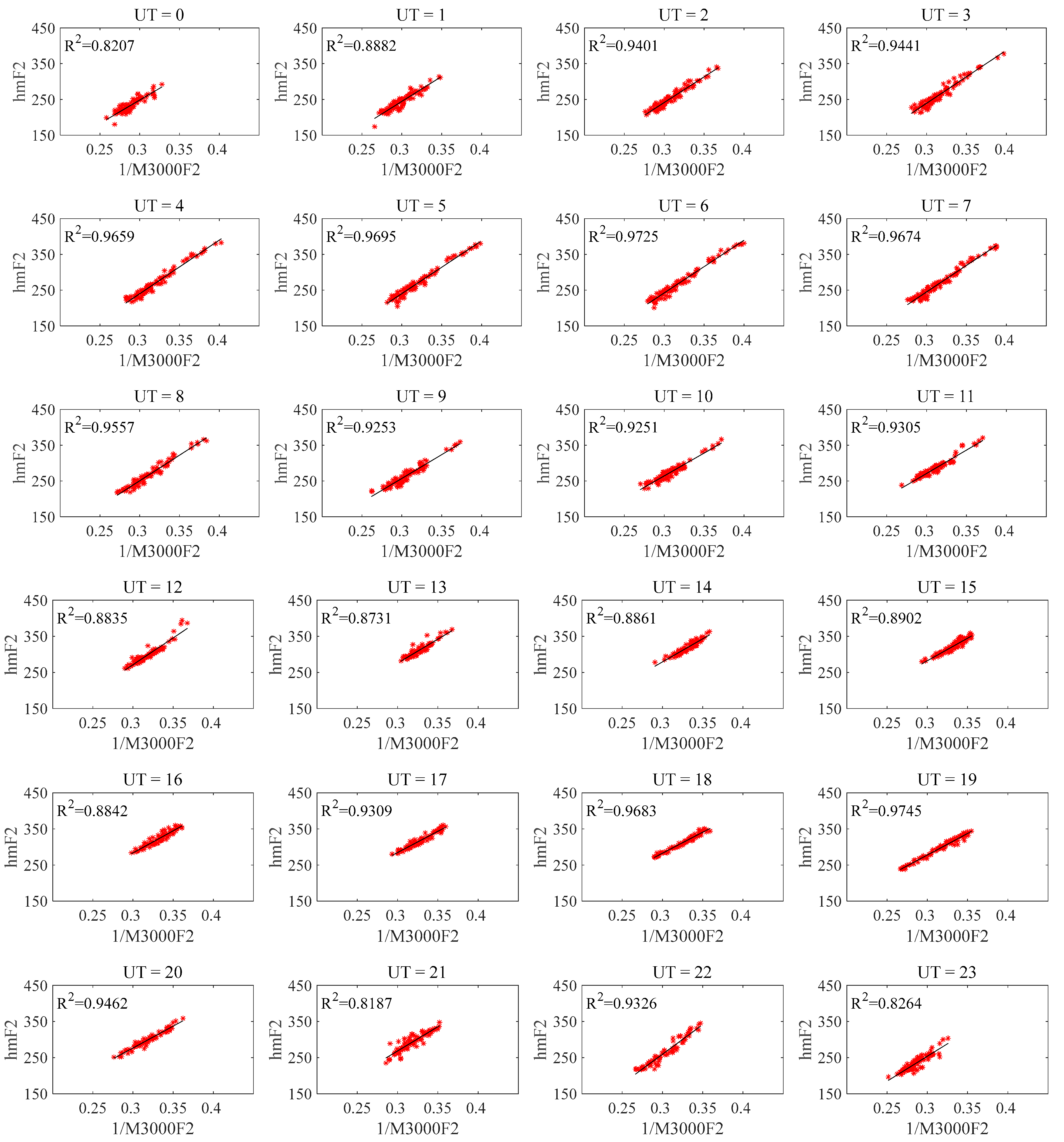
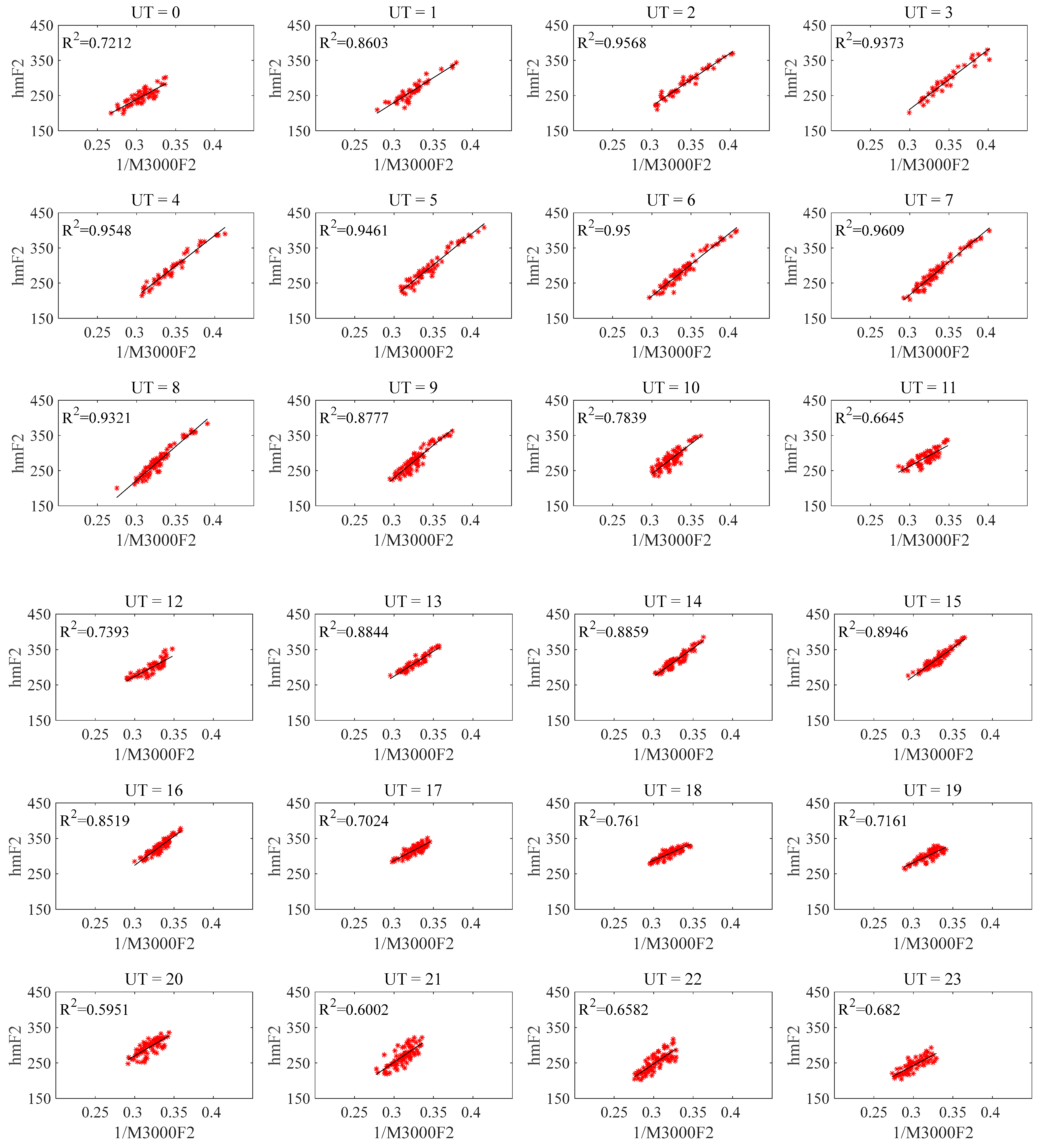
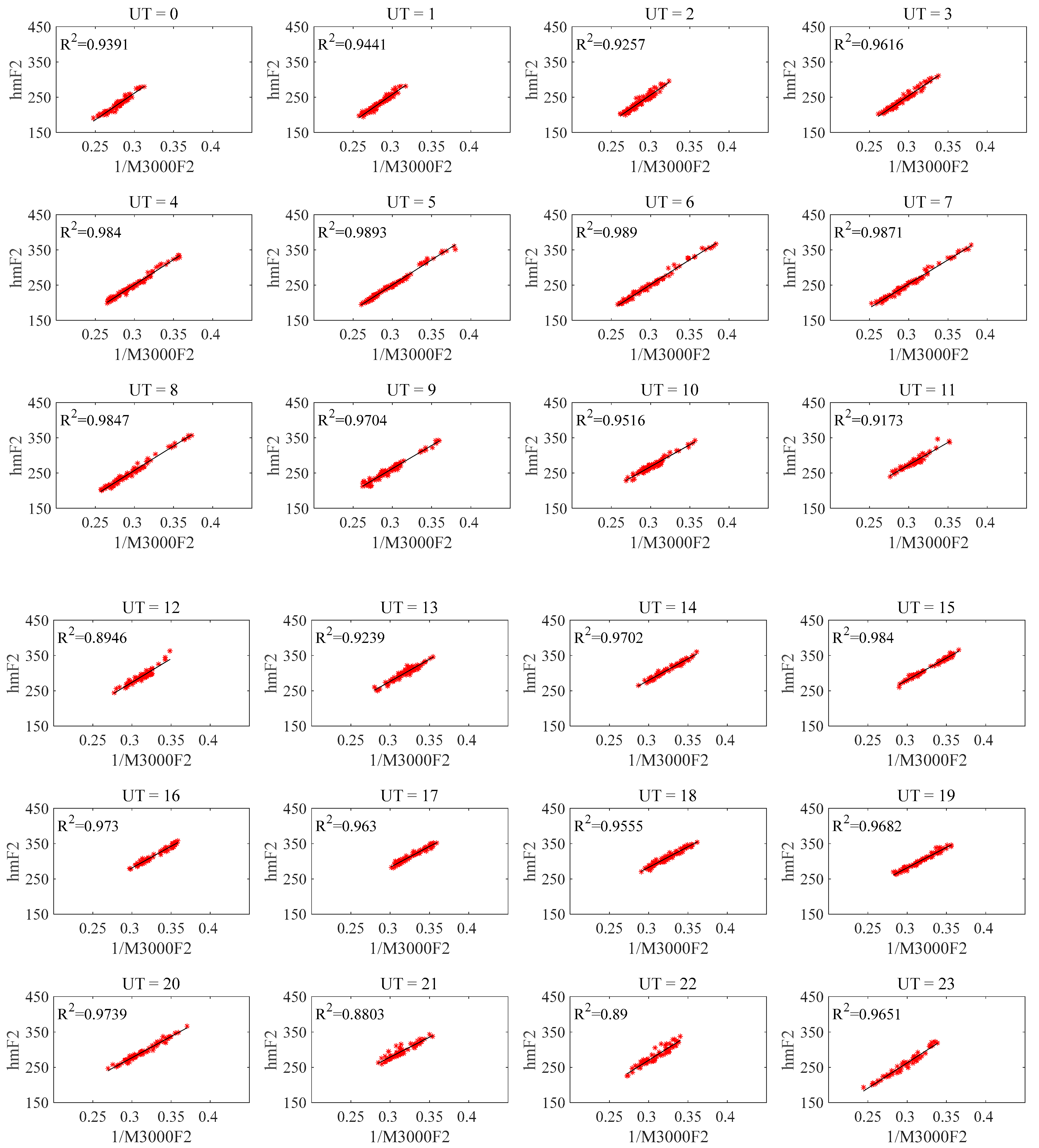
Figure 9, Figure 10 and Figure 11 show the training results under different UTs and seasons, which are equinox (corresponding to Figure 9), summer (corresponding to Figure 10), and winter (corresponding to Figure 11), and the corresponding R2 is labeled in the upper left corner of each subgraph.
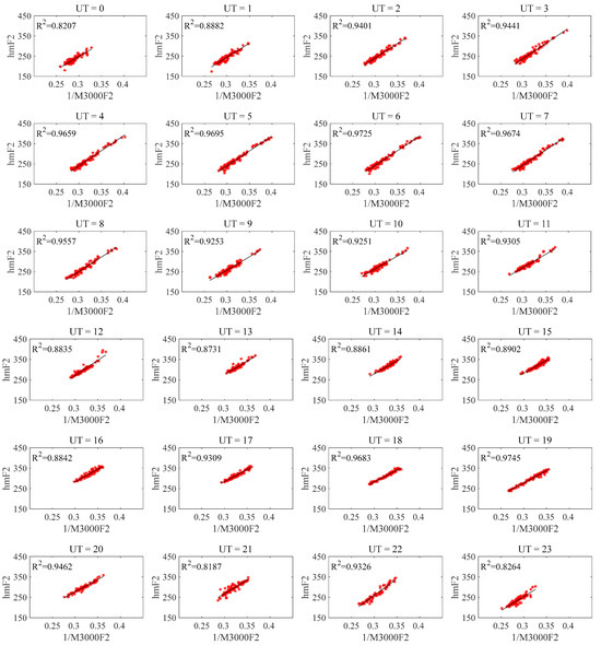
Figure 9.
The training result of equinox.
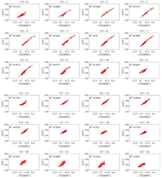
Figure 10.
The training result of the summer.
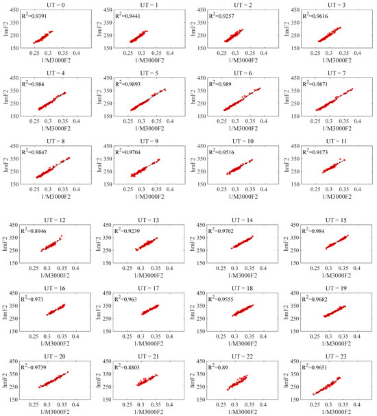
Figure 11.
The training result of winter.
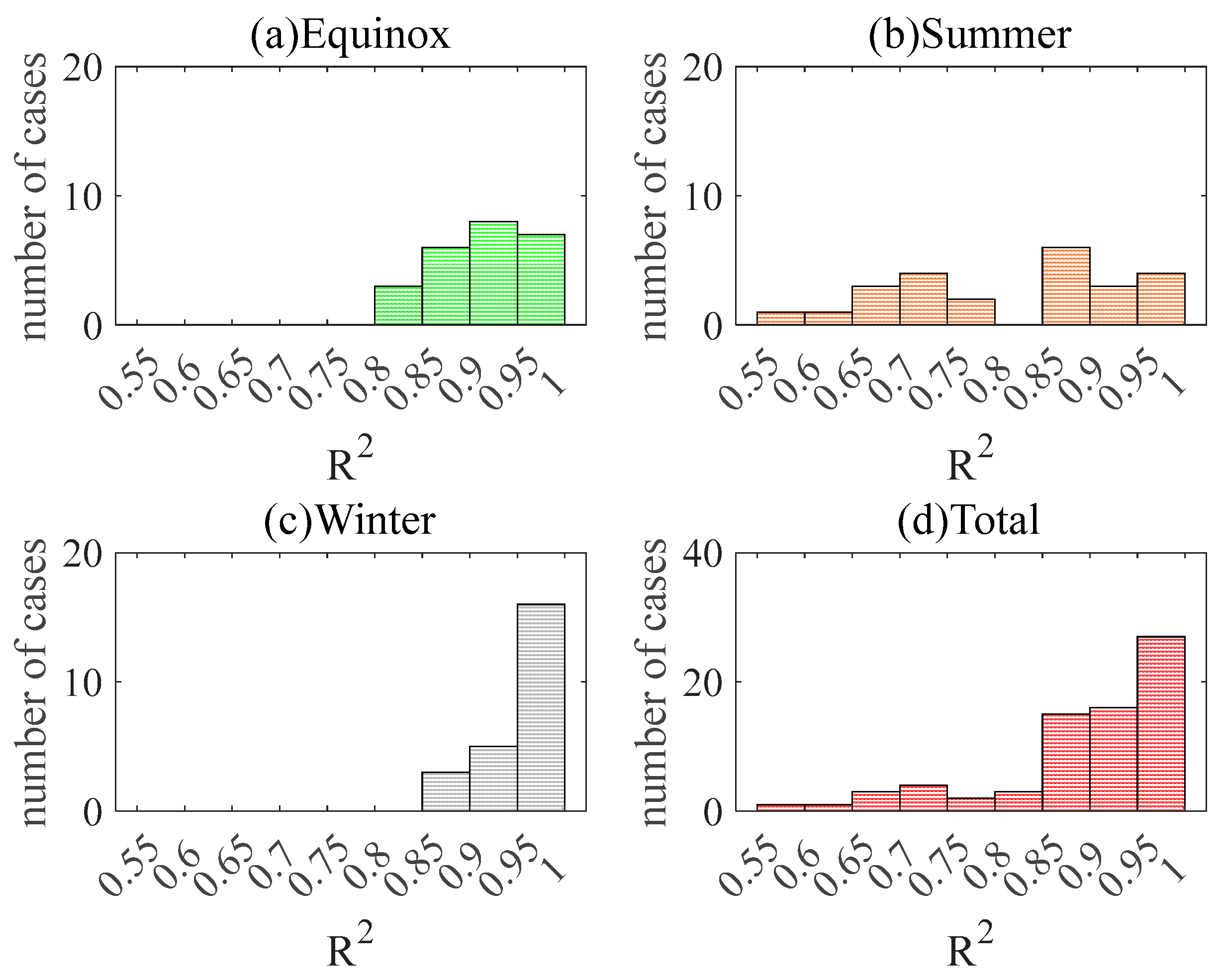
Figure 12 shows the distribution of R2 of different seasons. The horizontal coordinate represents the value of R2, and the vertical coordinate represents the number of events corresponding to R2. From Figure 9, Figure 10, Figure 11 and Figure 12, it can be seen that the goodness of fit in equinox and winter is better than the goodness of fit in summer. Among them, the R2 in equinox is between 0.8 and 1, the R2 in winter is between 0.85 and 1, and the R2 in summer is between 0.55 and 1. In summer, the R2 is 0.5951 when UT = 20 and 0.6002 when UT = 21. Except for the above two times, the corresponding R2 at other times is more significant than 0.65. This result shows that when M (3000) F2 is used to fit hmF2 according to season and UT, the fitting value is close to the measured value, which also proves the feasibility of this method.

Figure 12.
The histogram of R2: (a) Equinox; (b) Summer; (c) Winter; (d) Total.
4. Discussion
To test the generalization ability of the above-proposed model, we validate the trained model using validation data, the details of which are shown in Table 1. The validation data were substituted into the proposed model (identified as “PRO”) to obtain the predicted value. We compared the predicted value of the PRO model and the other three hmF2 models of IRI-2020 [12], which include Bilitza–Sheikh–Eyfrig (BSE) [18], Altadill–Magdaleno–Torta–Blanch (AMTB) [29] and Shubin (SHU) [30].
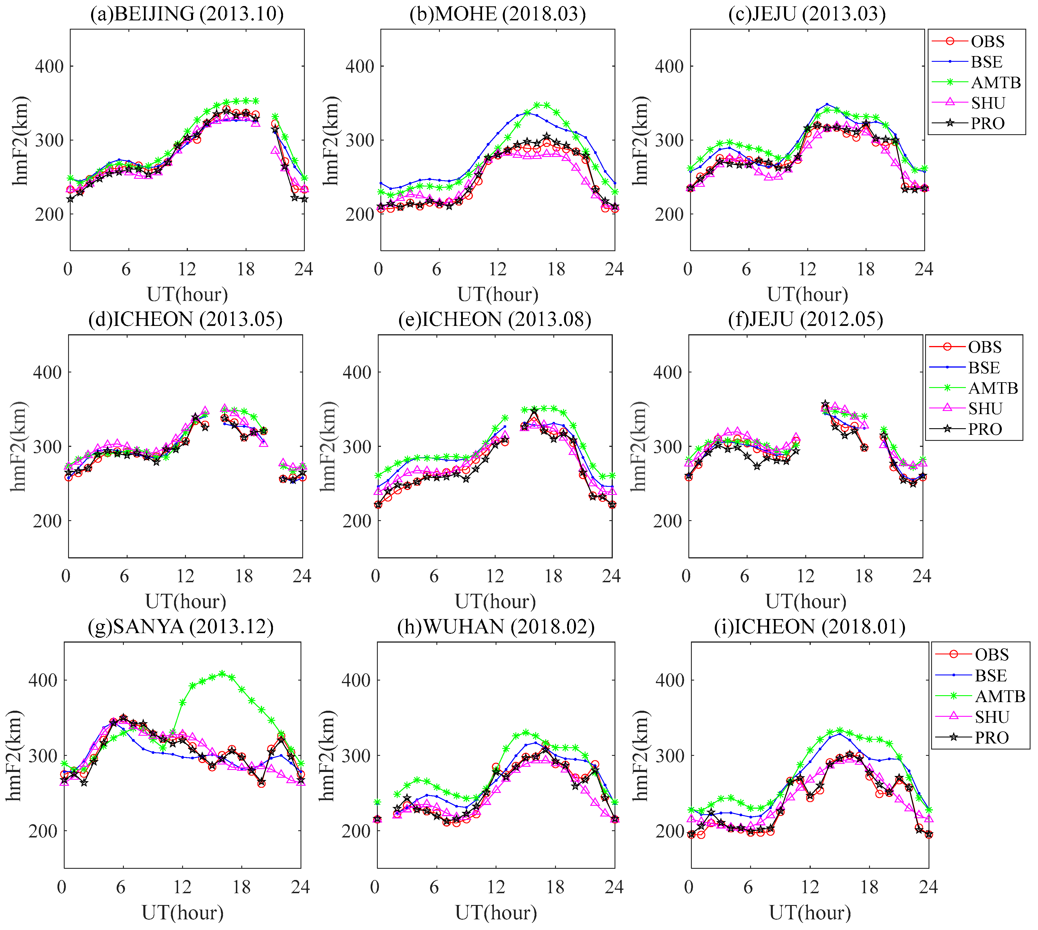
Figure 13 shows the specific data of observed hmF2 (OBS), the predicted value of three IRI models (BSE, AMTB, and SHU), and PRO. Each row represents a season, from top to bottom: equinox, summer, and winter. The results show that the PRO and OBS are closer than the IRI model. Moreover, PRO and OBS change trends are more consistent, as shown in Figure 13c,d,g–i, which can be consistent with the trend at the inflection point of OBS. Figure 13 also shows that there are differences in the forecasting performance of the same model at different times. For example, the prediction of the AMTB model for summer is significantly better than that of equinox and winter.
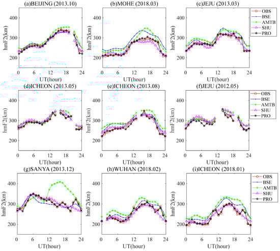
Figure 13.
Specific data of OBS, the predicted value of three IRI models (BSE, AMTB, and SHU), and PRO: (a) Beijing (2013.10); (b) Mohe (2018.03); (c) Jeju (2013.03); (d) Icheon (2013.05); (e) Icheon (2018.08); (f) Jeju (2012.05); (g) Sanya (2013.12); (h) Wuhan (2018.02); (i) Icheon (2018.01).
In order to show the advantages of the proposed model more precisely, RMSE and RRMSE between the predicted and observed values of the model were calculated according to (8) and (9), respectively, according to the season and the solar activity period.
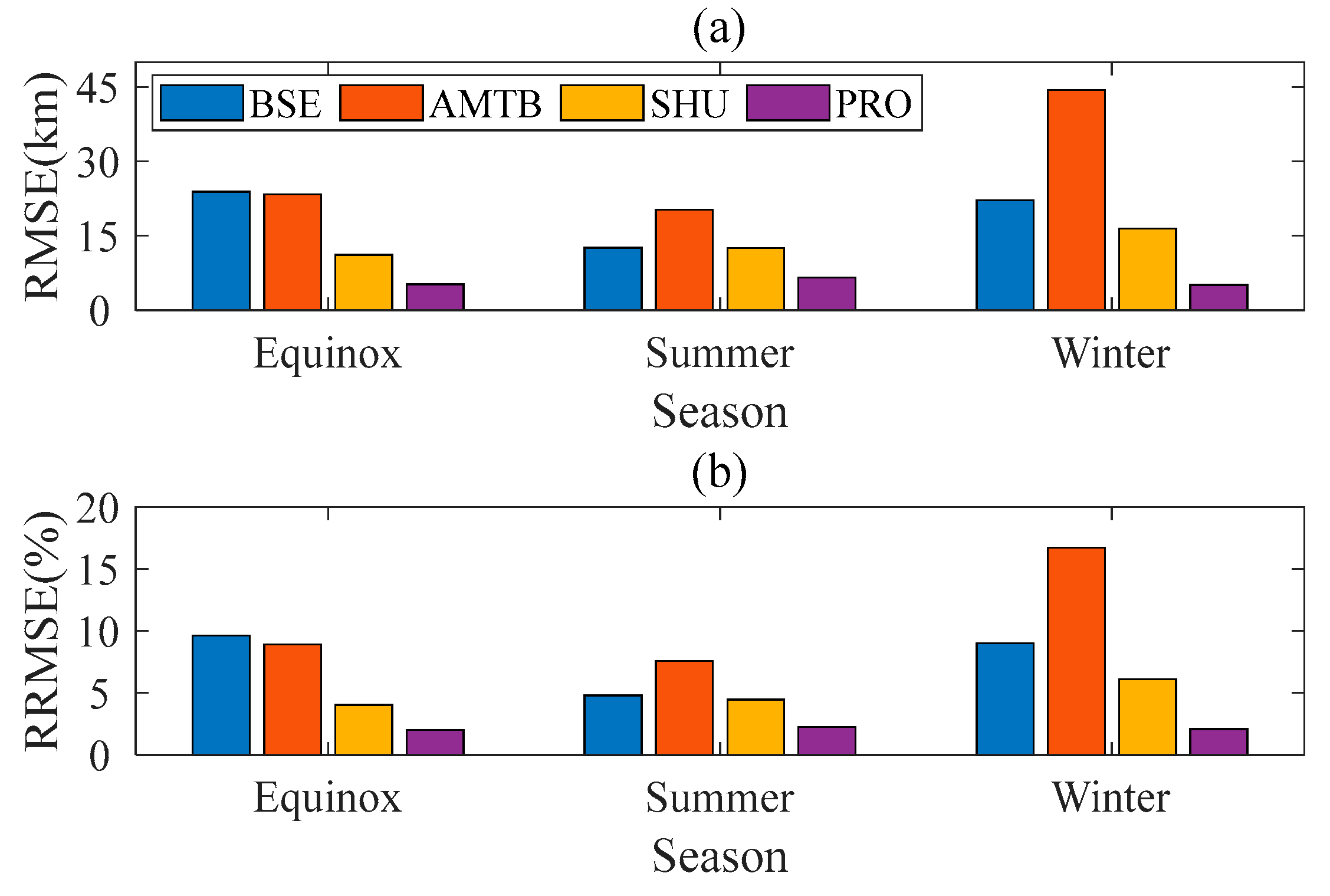
Figure 14 shows the error graphs of RMSE and RRMSE calculated according to seasons. The RMSEs of the PRO model in equinox, summer, and winter are 5.25 km, 6.61 km, and 5.12 km, respectively, and the RRMSEs of the PRO model are 2.02%, 2.26%, and 2.09%, respectively. Compared with other models, the proposed model showed absolute advantages in any season.

Figure 14.
The RMSE and RRMSE between the model’s predicted and observed values are calculated seasonally: (a) RMSE; (b) RRMSE.
Figure 15 shows the error graph of RMSE and RRMSE calculated according to the solar activity period. The RMSE and RRMSE of the PRO model are 5.82 km and 2.04%, respectively, in high solar activity years. During low solar activity years, the RMSE is 5.39 km and the RRMSE is 2.28%. Compared with other models, the RMSE and RRMSE of PRO are much smaller than the three models of IRI, whether in high or low solar activity years.
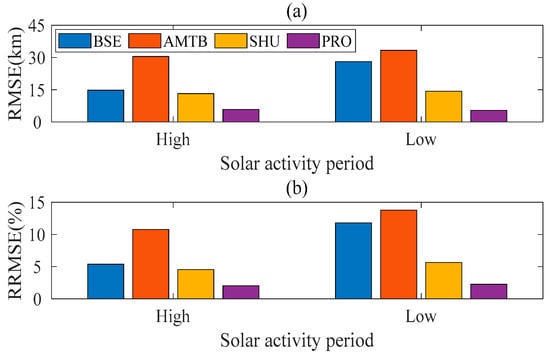
Figure 15.
The RMSE and RRMSE between the model’s predicted and observed values are calculated according to the solar activity period: (a) RMSE; (b) RRMSE.
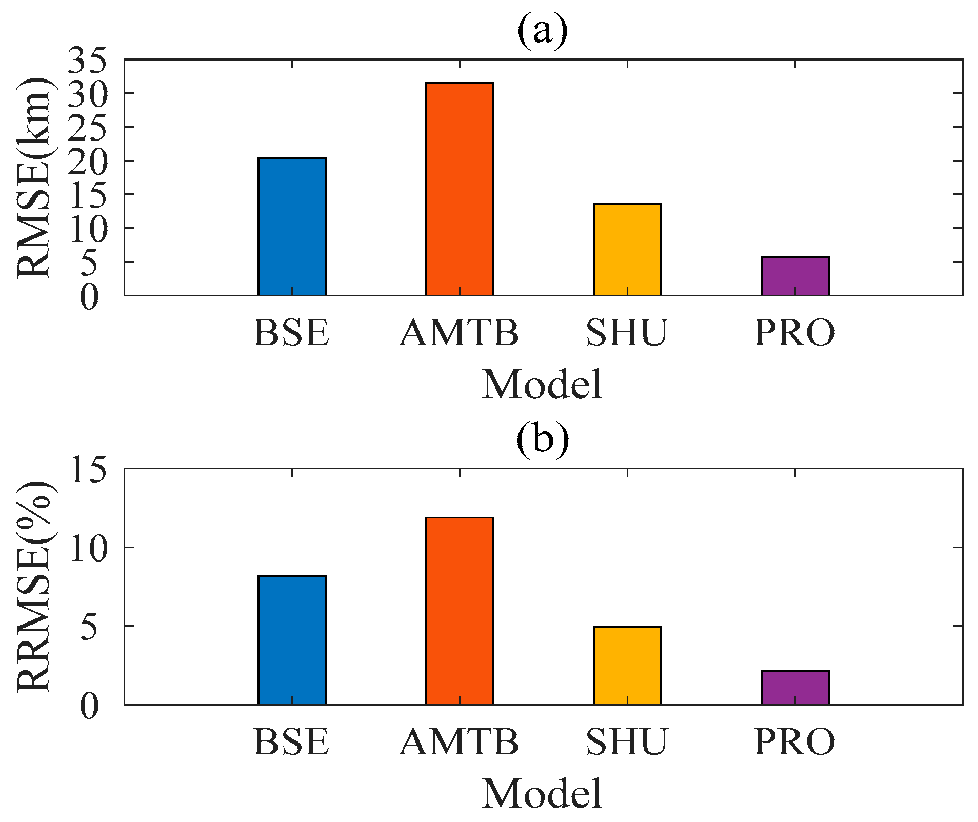
Figure 16 shows the statistics of RMSE and RRMSE, respectively, according to the model. The RMSE of BSE, AMTB, SHU, and PRO were 20.35 km, 31.51 km, 13.59 km, and 5.68 km, and the RRMSE of BSE, AMTB, SHU and PRO were 8.17%, 11.88%, 4.96%, and 2.12%, respectively. The above results showed that the PRO model was the most accurate predictor of hmF2, followed by the SHU model, and the AMTB model was the worst. Compared with the three IRI models, the RMSE of PRO decreased by 14.67 km, 25.83 km, and 7.91 km, and RRMSE decreased by 6.05%, 9.76%, and 2.84%, respectively. The above results show that, compared with the IRI model, the PRO model has a higher accuracy in long-term hmF2 prediction in east Asia. These results also prove the validity of the proposed model.

Figure 16.
RMSE and RRMSE between predicted and observed values were calculated according to the model: (a) RMSE; (b) RRMSE.
5. Conclusions
In this paper, according to the strong physical correlation between hmF2 and M(3000)F2, a new model to determine hmF2 is proposed: the model is trained according to season and universal time, and the physical expression of hmF2 and 1/M(3000)F2 is obtained. The feasibility of this method is proved by the calculation of correlation and goodness of fit. The method was verified in east Asia. The results showed that, compared with the three IRI models, the RMSE of the PRO model was reduced by 14.67 km, 25.83 km, and 7.91 km, and the RRMSE was reduced by 6.05%, 9.76%, and 2.84%, respectively. The PRO model had more minor errors and higher accuracy. In addition, compared with the three models of IRI, PRO is more accurate in predicting the turning point trend of hmF2.
The proposed model generally has the advantages of simple structure, convenient calculation, and better prediction accuracy than the IRI model. This paper provides a new idea to predict hmF2: improve the prediction accuracy of the ionospheric parameter M(3000)F2 and then improve the prediction accuracy of hmF2 according to the correlation between M(3000)F2 and hmF2. At the same time, the proposed method can obtain hmF2 at the corresponding time according to the measured M(3000)F2 and further expand the hmF2 data source. It is beneficial for planning and designing ionospheric high-frequency propagation systems, studying ionospheric mechanisms, and exploring space weather coupling law in this region.
At the same time, there are still some aspects which are worth exploring: (1) The data from 2012, 2013, and 2018 were selected for validation data, which were all near the training data (2014–2017), and the applicability of the model for other times needs to be studied; (2) This paper compares PRO with IRI model, and future work can be compared with other models.
Author Contributions
Conceptualization, J.W. and Q.Y.; methodology, J.W. and Q.Y.; software, J.W., Q.Y., Y.S. and Y.Z.; validation, J.W. and Q.Y.; formal analysis, J.W., Q.Y. and Y.S.; investigation, J.W., Q.Y., Y.S. and Y.Z.; resources, J.W., Q.Y. and Y.Z.; data curation, J.W. and Q.Y.; writing—original draft preparation, J.W. and Q.Y.; writing—review and editing, J.W., Q.Y., Y.S., C.Y., S.J. and Y.Z.; visualization, J.W., Q.Y., S.J. and Y.Z.; supervision, J.W., Q.Y. and Y.S.; project administration, J.W. and Y.Z.; funding acquisition, J.W. and Y.Z. All authors have read and agreed to the published version of the manuscript.
Funding
This research was funded by the State Key Laboratory of Complex Electromagnetic Environment Effects on Electronics and Information Systems (No. CEMEE2022G0201).
Data Availability Statement
Data are contained within the article.
Conflicts of Interest
The authors declare no conflict of interest.
References
- Zhang, B.; Wang, Z.; Shen, Y.; Li, W.; Xu, F.; Li, X. Evaluation of foF2 and hmF2 Parameters of IRI-2016 Model in Different Latitudes over China under High and Low Solar Activity Years. Remote Sens. 2022, 14, 860. [Google Scholar] [CrossRef]
- Wang, J.; Yang, C.; An, W. Regional Refined Long-Term Predictions Method of Usable Frequency for HF Communication Based on Machine Learning Over Asia. IEEE Trans. Antennas Propag. 2022, 70, 4040–4055. [Google Scholar] [CrossRef]
- Wang, J.; Shi, Y.; Yang, C.; Zhang, Z.; Zhao, L. A Short-Term Forecast Method of Maximum Usable Frequency for HF Communication. IEEE Trans. Antennas Propag. 2023, 71, 5189–5198. [Google Scholar] [CrossRef]
- Fagre, M.; Zossi, B.S.; Chum, J.; Yiğit, E.; Elias, A.G. Ionospheric high frequency wave propagation using different IRI hmF2 and foF2 models. J. Atmos. Sol. Terr. Phys. 2019, 196, 105141. [Google Scholar] [CrossRef]
- Liu, Y.; Yu, Q.; Shi, Y.; Yang, C.; Wang, J. A Reconstruction Method for Ionospheric foF2 Spatial Mapping over Australia. Atmosphere 2023, 14, 1399. [Google Scholar] [CrossRef]
- Schunk, R.; Nagy, A. Ionospheres: Physics, Plasma Physics, and Chemistry; Cambridge University Press: Cambridge, UK, 2009. [Google Scholar]
- Elias, A.G.; Zossi, B.S.; Yiğit, E.; Saavedra, Z.; Barbas, B.F.H. Earth’s magnetic field effect on MUF calculation and consequences for hmF2 trend estimates. J. Atmos Sol. Terr. Phy. 2017, 163, 114–119. [Google Scholar] [CrossRef]
- Huang, H.; Moses, M.; Volk, A.E.; Elezz, O.A.; Kassamba, A.A.; Bilitza, D. Assessment of IRI-2016 hmF2 model options with digisonde, COSMIC and ISR observations for low and high solar flux conditions. Adv. Space Res. 2021, 68, 2093–2103. [Google Scholar] [CrossRef]
- Sezen, U.; Sahin, O.; Arikan, F.; Arikan, O. Estimation of hmF2 and foF2 Communication Parameters of Ionosphere F2 -Layer Using GPS Data and IRI-Plas Model. IEEE Trans. Antennas Propag. 2013, 61, 5264–5273. [Google Scholar] [CrossRef]
- Maruyama, T.; Ma, g.; Tsugawa, T.; Supnithi, P.; Komolmis, T. Ionospheric peak height at the magnetic equator: Comparison between ionosonde measurements and IRI. Adv. Space Res. 2017, 60, 375–380. [Google Scholar] [CrossRef]
- Thu, H.; Mazaudier, C.; Huy, M.; Thanh, D.; Viet, H.; Thi, N.; Hozumi, K.; Truong, T. Comparison between IRI-2012, IRI-2016 models and F2 peak parameters in two stations of the EIA in Vietnam during different solar activity periods. Adv. Space Res. 2021, 68, 2076–2092. [Google Scholar] [CrossRef]
- Bilitza, D.; Pezzopane, M.; Truhlik, V.; Altadill, D.; Reinisch, B.W.; Pignalberi, A. The International Reference Ionosphere model: A review and description of an ionospheric benchmark. Rev. Geophys. 2020, 60, e2022RG000792. [Google Scholar] [CrossRef]
- Zhang, X.; Jiang, C.; Liu, T.; Yang, G.; Zhao, Z. Effect of the ionospheric virtual height on the joint positioning accuracy of multi-station over-the-horizon radar system. Chin. J. Radio Sci. 2022, 37, 761–767. [Google Scholar]
- Fatima, T.; Ameen, M.A.; Jabbar, M.A.; Baig, M.J. The variation of ionosonde-derived hmF2 and its comparisons with International Reference Ionosphere (IRI) and Empirical Orthogonal Function (EOF) over Pakistan longitude sector during solar cycle 22. Adv. Space Res. 2021, 68, 2104–2114. [Google Scholar] [CrossRef]
- Tang, J.; Ji, S.; Wang, J.; Wang, X. Assimilation methods of ionospheric short-term forecast for selecting frequency in short wave communication. Chin. J. Radio Sci. 2022, 28, 499–504. [Google Scholar]
- Adebesin, B.O.; Adeniyi, J.O. F2-layer height of the peak electron density (hmF2) dataset employed in Inferring Vertical Plasma Drift–Data of Best fit. Data Brief 2015, 19, 59–66. [Google Scholar] [CrossRef]
- Shimazaki, T. World-wide daily variations in the height of the electron density of the ionospheric F2-layer. J. Radio Res. Lab. 1955, 2, 85–97. [Google Scholar]
- Bradley, P.A.; Dudeney, J.R. A simple model of the vertical distribution of electron concentration in the ionosphere. J. Atmos. Solar. Terr. Phys. 1973, 35, 2131–2146. [Google Scholar] [CrossRef]
- Dudeney, J.R. A Simple Empirical Method for Estimating the Height and Semi-Thickness of the F2-Layer at the Argentine Islands Graham Land; Science Report 88; British Antarctic Survey: London, UK, 1975. [Google Scholar]
- Bilitza, D.; Eyfrig, R.; Sheikh, A.M. A global model for the height of the F2-peak using M3000 values from the CCIR numerical map. ITU Telecommun. J. 1979, 49, 549–553. [Google Scholar]
- Adebesin, B.O.; Adeniyi, J.O.; Afolabi, P.A.; Ikubanni, S.O.; Adebiyi, S.E. Modelling M(3000)F2 at an African equatorial location for better IRI-model prediction. Radio Sci. 2022, 57, 1–19. [Google Scholar] [CrossRef]
- Oyekola, O.S. Comparison of IRI-2016 model-predictions of F2-layer peak density height options with the ionosonde-derived hmF2 at the equatorial station during different phases of solar cycle. Adv. Space Res. 2019, 64, 2064–2076. [Google Scholar] [CrossRef]
- Brunini, C.; Conte, J.F.; Azpilicueta, F.; Bilitza, D. A different method to update monthly median hmF2 values. Adv. Space Res. 2013, 51, 2322–2332. [Google Scholar] [CrossRef]
- Sugiyama, M. Statistical Machine Learning; China Machine Press: Beijing, China, 2016. [Google Scholar]
- Lu, X.; Song, J. Big Data Mining and Statistical Machine Learning; China Renmin University Press: Beijing, China, 2016. [Google Scholar]
- Wang, J.; Shi, Y.; Yang, C. Investigation of Two Prediction Models of Maximum Usable Frequency for HF Communication Based on Oblique- and Vertical-Incidence Sounding Data. Atmosphere 2022, 13, 1122. [Google Scholar] [CrossRef]
- Lloyd, H. A Treatise on Magnetism General and Terrestrial by Humphrey Lloyd; Longmans, Green and Company: London, UK, 1874. [Google Scholar]
- Bello, S.A.; Abdullah, M.; Hamid, N.S.A.; Yusuf, K.A.; Yoshikawa, A.; Fujimoto, A. Fujimoto, Robust least square modelling for selected daytime ionospheric parameters using geomagnetic observations at low latitudes. Adv. Space Res. 2023, 72, 1615–1633. [Google Scholar] [CrossRef]
- Altadill, D.; Magdaleno, S.; Torta, J.M.; Blanch, E. Global empirical models of the density peak height and of the equivalent scale height for quiet conditions. Adv. Space Res. 2013, 52, 1756–1769. [Google Scholar] [CrossRef]
- Shubin, V.N. Global median model of the F2-layer peak height based on ionospheric radio-occultation and ground-based Digisonde observations. Adv. Space Res. 2015, 56, 916–928. [Google Scholar] [CrossRef]


Disclaimer/Publisher’s Note: The statements, opinions and data contained in all publications are solely those of the individual author(s) and contributor(s) and not of MDPI and/or the editor(s). MDPI and/or the editor(s) disclaim responsibility for any injury to people or property resulting from any ideas, methods, instructions or products referred to in the content. |
© 2024 by the authors. Licensee MDPI, Basel, Switzerland. This article is an open access article distributed under the terms and conditions of the Creative Commons Attribution (CC BY) license (https://creativecommons.org/licenses/by/4.0/).