Abstract
There have been considerable efforts in generating tree crown maps from satellite images. However, tree localization in urban environments using satellite imagery remains a challenging task. One of the difficulties in complex urban tree detection tasks lies in the segmentation of dense tree crowns. Currently, methods based on semantic segmentation algorithms have made significant progress. We propose to split the tree localization problem into two parts, dense clusters and single trees, and combine the target detection method with a procedural generation method based on planting rules for the complex urban tree detection task, which improves the accuracy of single tree detection. Specifically, we propose a two-stage urban tree localization pipeline that leverages deep learning and planting strategy algorithms along with region discrimination methods. This approach ensures the precise localization of individual trees while also facilitating distribution inference within dense tree canopies. Additionally, our method estimates the radius and height of trees, which provides significant advantages for three-dimensional reconstruction tasks from remote sensing images. We compare our results with other existing methods, achieving an 82.3% accuracy in individual tree localization. This method can be seamlessly integrated with the three-dimensional reconstruction of urban trees. We visualized the three-dimensional reconstruction of urban trees generated by this method, which demonstrates the diversity of tree heights and provides a more realistic solution for tree distribution generation.
1. Introduction
As urban greenery, forest cities, and urban ecological civilization have gained increasing attention, the number of trees in cities has been rising year by year. According to statistics, globally, 186 million hectares of forests are designated for social services, and since 2010, the area of forests designated for this purpose has been growing at a rate of 186,000 hectares per year [1]. This represents a continuous increase in the coverage and diversity of urban trees, resulting in an increase in the complexity of urban tree management. The detailed information on tree quantity and distribution will provide valuable references for urban infrastructure safety, city planning, sustainable development, and natural resource management [2,3,4]. Therefore, how to accurately count and manage these trees will be the focus of future urban green development. For the recent development of three-dimensional urban modeling and smart city management, the localization and estimation of tree positions and radii are indispensable pieces of information. Consequently, more and more efforts are being dedicated to the statistical analysis of urban trees.
Traditional methods still require on-site surveys, such as the U.S. Department of Agriculture’s i-Tree 6.1 software package. These methods have long update cycles and consume significant resources, exceeding the accuracy requirements and resource investment of three-dimensional reconstruction tasks. Satellite images can achieve the rapid monitoring of forests on a large scale and at low cost, but currently they are mainly used for large-scale low-precision forest monitoring [5,6]. This method is inefficient for trees outside the forest and ignores the diversity of individual trees, which often have variable heights and crown sizes [7,8].
With the increasing quality of remote sensing images, high-resolution optical images have become more suitable for research. These high-resolution images have enabled the use of deep learning methods. Martin Brandt et al. [9] have used semantic segmentation methods to segment billions of trees and shrubs in the Sahelian savannah and Sub-Saharan desert landscapes, indicating the feasibility of deep learning methods for the large-scale detection of isolated trees. However, in urban environments, there are not only a large number of isolated trees, but also a large number of enclosed forests and complex combinations of tree planting. This has made past methods still focus on the segmentation of tree crowns in remote sensing images. These methods can be roughly divided into two categories. The first category of methods [10] uses semantic segmentation networks to obtain edge maps of tree crowns and combines them with heat maps to distinguish different tree crowns. These methods have high requirements on the gaps between tree crowns in remote sensing images when generating edge maps, and they perform poorly when dealing with dense tree crowns. The second category of methods [11,12] first obtains a tree crown coverage map of the input image and then uses a generative algorithm to generate the distribution of trees for the covered areas. These methods treat all tree crowns as a whole and generate the distribution of trees, which can result in some isolated tree crowns being generated as multiple trees.
Through observation, we found that isolated trees account for a significant proportion of urban tree distribution, especially in residential areas, where they account for up to 38%. Therefore, to improve the detection accuracy of isolated trees, we used target detection methods to detect them. We also divided urban trees into three units: clusters of trees, individual trees, and low shrubs to adapt to the complexity of urban tree distribution. To make the results closer to the real distribution, we also considered the impact of two attributes on tree distribution. First is the urban area attribute. In previous methods [12], this step required manual determination, and there were differences in the division of different urban areas. We propose an automatic urban area division algorithm that divides urban areas based on the species and area characteristics of ground objects. Second is the crown size attribute. Previous methods [12] used a Poisson distribution for all forested areas, resulting in a single crown size, which does not match the complex distribution of tree combinations in urban environments. We referenced the design concept of [13], and proposed an urban tree generation algorithm based on planting rules to make the generated results closer to the real distribution. Like the method of Till et al. [11], we used tree location to describe the distribution of trees. This method is not affected by the fuzzy boundaries of tree crowns and provides seamless integration for subsequent 3D reconstruction visualization due to its sparse representation.
The main contributions of this paper are as follows:
- Incorporating object detection methods firstly and combining them with semantic segmentation for tree localization tasks, dividing the detection targets into easily detectable individual trees, shrub units, and challenging tree clusters, achieving the highest accuracy in individual tree detection;
- Developing a planting rule algorithm based on forest characteristics to more realistically represent the distribution of tree clusters;
- Designing a city region partition algorithm that automatically divides the urban space into four categories;
- Estimating the positions, radii, heights, and other information of trees from satellite images and utilizing this information in three-dimensional reconstruction to create more realistic models of urban trees compared to previous methods.
2. Materials
Related work includes traditional methods for obtaining tree information, the application of deep learning in tree information retrieval, and the use of procedural generation for tree distribution.
2.1. Traditional Methods for Obtaining Tree Information
In the past, field surveys were the primary means of obtaining tree information. Crowther [14] used plot-based methods to estimate tree quantity globally, while Nowak [15] employed field surveys to create urban tree canopy maps. However, these methods often required a significant amount of manpower and were challenging to dynamically monitor tree changes.
Edson [16], using Lidar technology, effectively obtained tree height, positioning, and other information. Still, this approach’s high cost limited its widespread application. With the improvement in optical image resolution, the focus of methods has gradually shifted. Wang [17] used watershed segmentation algorithms to detect the edges of isolated trees for obtaining tree crown information. Martins [18] proposed a superpixel-based method for forest detection, while Culvenor [19] used spectral-based approaches to distinguish tree crown centers and boundaries.
While traditional methods maintain accuracy in small-scale forest areas, they face challenges in large-scale tree information retrieval. These challenges include the need for generalization across diverse tree types, adaptability to complex environments, and heavy reliance on manual efforts. As a result, there is an increasing interest in exploring new approaches, particularly those based on deep learning techniques, to overcome these limitations and improve the efficiency and effectiveness of tree information retrieval.
2.2. Application of Deep Learning in Tree Information Retrieval
Since the introduction of machine learning and deep learning, there has been a significant amount of work applying these techniques to tree detection-related fields. Some studies have utilized unmanned aerial vehicle (UAV) images for this purpose. For example, Ghasemi et al. [20] used Support Vector Machines (SVMs) to detect and delineate the canopies of declining trees, while Han et al. [21] proposed a framework algorithm embedded in UAVs for tree counting from continuous aerial images. Onishi et al. [22] applied CNN-based methods to classify trees in drone images and achieved good results. Firoze et al. [23] proposed a novel forest instance segmentation scheme using continuous image sequences from UAVs. However, UAV images are only suitable for small-scale vegetation detection, and compared to aerial images, they require higher investment costs, making them less applicable for large-scale urban vegetation detection.
In the field of aerial imagery, due to the presence of dense forest canopies, it is challenging to easily distinguish the boundaries of individual trees. Therefore, semantic segmentation is the most commonly used method for tree detection tasks. Martin Brandt et al. [9] used a method based on Unet to perform tree detection over large-scale regions in West Africa’s Sahel and Sahara areas, estimating the number of trees in that region. Guo et al. [24] used the Deeplabv3 network and incorporated semi-supervised learning for generating urban tree canopy maps across Brazil on a national scale. However, these methods can only generate rough tree canopy coverage maps and cannot differentiate between different tree crowns. Maximilian [10] proposed a new Unet-based method, where the network generates tree crown edges and heatmaps, which are then combined to output different tree crown regions, allowing for better distinction between trees. On the other hand, Liu et al. [25] treated tree counting as a density regression task and introduced TreeCountNet, which generates tree crown density maps from remote sensing images and uses them to obtain the total number of trees within a specified region. Li et al. [26] used aerial images and Lidar data to perform tree segmentation, counting, and height prediction at the national scale, which differs from the task we are considering in this article, which focuses on single optical remote sensing images.
However, it is essential to note that object detection has rarely been applied in this research direction. Using object detection to distinguish trees in remote sensing images has often been considered impossible. Yang et al. [27] managed to achieve tree crown delineation in small-scale areas within New York’s Central Park using a Mask-RCNN-based method. Indeed, after the introduction of transformers in image processing, object detection algorithms have made significant advancements in recent times. Subsequent methods such as Swin Transformer [28] and DETR [29] have further developed excellent object detection algorithms. Our TreeDetector is based on the DETR [29] method, and the results show that current object detection algorithms can effectively distinguish the three vegetation units defined in our study—individual trees, tree clusters, and shrubs.
2.3. Application of Procedural Generation in Tree Distribution
The deep learning methods mentioned earlier [9,24] mostly focused on tree crown segmentation, without paying much attention to specific tree localization and more detailed information, such as tree radius. These detailed pieces of information are crucial for tree management and 3D reconstruction. Procedural generation has been used in urban modeling for a long time [30,31,32], saving many tedious manual steps. However, very few works [33] have addressed its application to tree distribution within urban environments. Niese et al. [11] proposed a Procedural Planting Model (PPM) for urban vegetation layout. With this model, users can generate vegetation distribution by defining various parameters. They also made some simple attempts with deep learning methods. Building on this work, Firoze [12] made several improvements and introduced a solution that combines deep learning with procedural generation. They used a segmentation network to generate tree crown coverage maps and trained a GAN network with procedurally generated synthetic data to generate tree positions. This approach proved to be effective, but it requires additional supporting information, and the general rules may not generate reasonable tree distributions for each specific area. Moreover, it may lead to misclassifying larger individual trees as multiple trees.
In urban modeling, land is often divided into different functional zones, such as urban areas, suburbs, industrial zones, etc. Benes et al. [34] proposed “urban brush”, which defines different urban styles to distinguish these regions. Similarly, when applying procedural generation to tree distribution, the task of automatic region classification becomes crucial. Firoze [12] addressed this issue by performing semantic segmentation and then using clustering methods to separate different urban regions. However, this process still required manual annotation for different areas. In practice, when information about buildings, roads, and vegetation in an image is available, it is indeed possible to define region classification for vegetation distribution. This is also one of the contributions of this paper—achieving automatic region classification based on the vegetation distribution, leveraging the information about buildings, roads, and vegetation in the image.
3. Methods
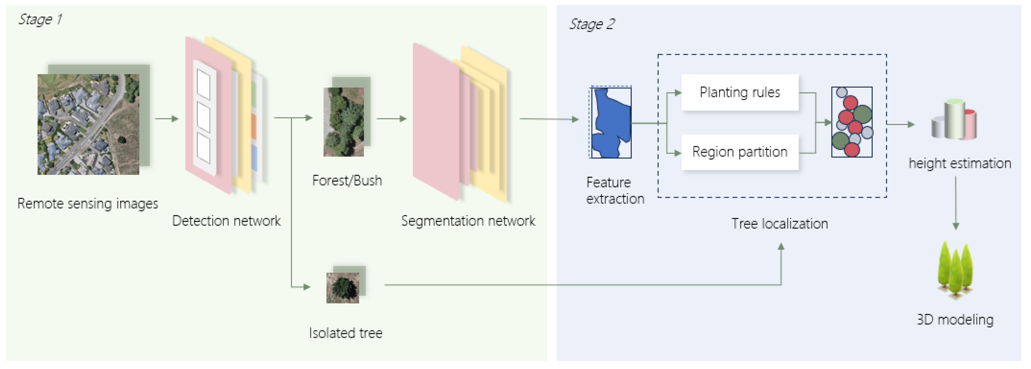
Our method consists of two stages (as shown in Figure 1). In the first stage, we use two trained neural networks to extract vegetation information from the input images. In the second stage, we employ procedural planting rules to obtain tree information, resulting in the final output of tree localization, radius, height, and other relevant details from the image.
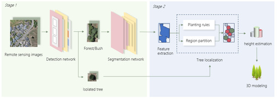
Figure 1.
The workflow diagram from input images to 3D modeling. In the first stage, the input remote sensing images go through an object detection neural network to identify three types of tree units. The tree clusters and low shrubs are then passed to the segmentation network to obtain their respective segmentation images. In the second stage, we start by extracting features from the segmentation images. Next, we apply region partitioning and planting rule algorithms to determine the positions of the trees. Finally, after estimating the tree heights, the 3D modeling is performed.
3.1. Definition of Tree Units
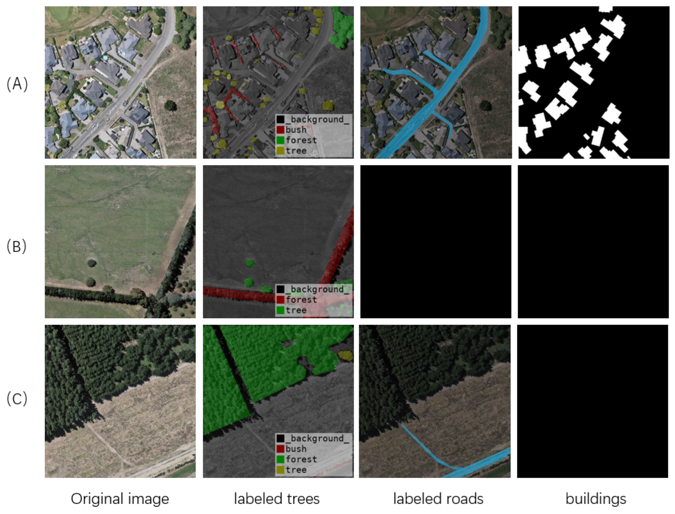
Unlike other tree detection methods [10,12], our proposed approach does not directly employ semantic segmentation for image processing. Instead, we initiate the process by using an object detection network to identify target objects. Furthermore, in contrast to some methods that directly detect individual trees [27], we adopt a novel approach for object detection. Historically, the approach of using object detection methods for tree detection mainly focused on isolated trees with regular distribution patterns, often in simpler surrounding scenes, such as plantations or arid regions [35,36]. In such cases, object detection networks can perform well in completing the task. However, in urban areas, tree distribution is often complex, characterized by various combinations of tree types. Additionally, remote sensing images captured during different seasons can exhibit significant variations. In Figure 2C, even the human eye struggles to distinguish boundaries between trees within dense clusters. This complexity makes annotating datasets using object detection methods extremely challenging—even with accurate datasets, current object detection algorithms struggle to differentiate trees within such highly complex and low-contrast clusters. This is why most urban vegetation analysis methods [10,12] avoid using object detection approaches. Our focus is on how to address complex tree distribution in urban environments using smaller datasets, reducing the annotation burden while effectively handling the challenges posed by intricate urban settings.
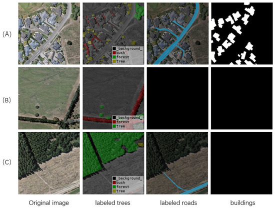
Figure 2.
Different annotation data. In (A), we show the annotation of residential areas. This image contains three types of tree units and includes roads and buildings. Part (B) primarily features densely arranged tree clusters and does not include roads or buildings. In (C), there are large clusters of dense forests, and we consider them as a whole.
J. Blum proposed that humans shape tree communities based on preferences at various spatial scales, whether in urban or residential areas. Each cluster of trees is often driven by specific factors [37]. Therefore, our method differentiates between continuous tree distribution clusters. We propose breaking down complex urban tree distributions into three distinguishable tree units, individual trees, tree clusters, and low shrubs as shown in the illustration below. With this approach, the object detection network can effectively distinguish between different types of tree units in input images, significantly reducing the required manual annotation effort. One major issue with using semantic segmentation networks in the past [10] was that, during the process of large-scale tree detection, although accuracy in tree coverage was ensured, it often resulted in reduced accuracy in identifying individual trees. This led to subsequent tree statistics having errors, such as mistakenly identifying single trees as regions composed of multiple trees or missing detections altogether. On the other hand, employing an object detection network that targets tree units can significantly enhance the accuracy of locating individual trees. This aspect holds significant importance for tasks like three-dimensional reconstruction, which aims to faithfully represent the urban vegetation landscape.
During our annotation process, we adhere to three key guidelines: (1) Aim to annotate all tree regions, disregarding excessively small trees. The minimum crown radius considered for trees in our study is 1.5 m. That means any trees larger than this scale will be included in our detection requirements. (2) Label complex tree clusters and densely spaced trees that are difficult to differentiate with the naked eye as “tree clusters”. (3) Label low and shrubby vegetation regions as “bushes”.
Our dataset is derived from the publicly available WHU Building Dataset by Wuhan University. This dataset covers an area of 450 km2 in Christchurch, New Zealand, and comprises over 9000 aerial images with a ground resolution of 0.3 m. These images are segmented into 512 × 512-sized segments and also include manually annotated building regions. In addition to tree annotations as mentioned earlier, we also annotated road areas. The annotation of roads and building regions aids in segmenting the image areas. It is important to note that current deep learning algorithms for image recognition of buildings and roads are quite mature. Therefore, this paper does not extensively focus on these aspects. In addition, when annotating, we choose not to count shadows, focusing instead on the bright crown part to avoid larger errors caused by the calculation of shadows. We annotated a total of 183 remote sensing images using Labelme and expanded them to 732 images using data augmentation. In Figure 2, we illustrate different annotation data.
3.2. Deep Learning Network Treedetector
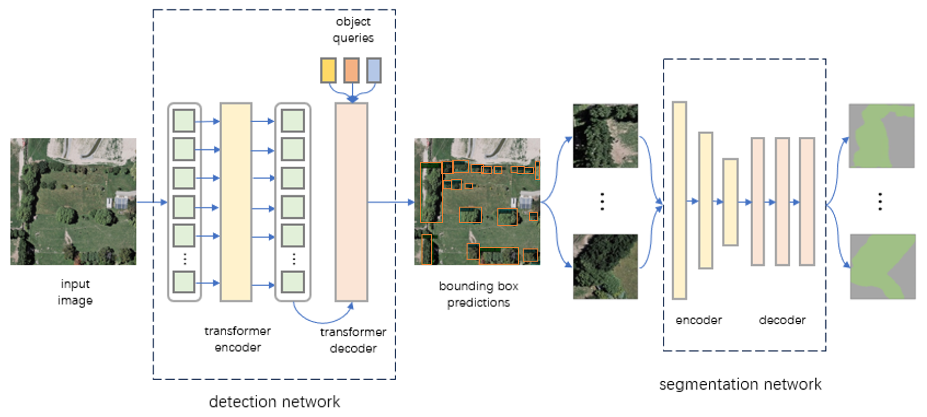
In Figure 3, we demonstrate how we employ neural networks to detect features in remote sensing images. Our approach involves utilizing an object detection network to approximate the general locations of all trees. Subsequently, a semantic segmentation network is applied to obtain detailed areas. This section will delve into the specifics of these networks.

Figure 3.
Obtaining tree units using neural networks. In this diagram, the input remote sensing image first passes through an object detection neural network. After obtaining the objects and classifying them, we extract these objects and feed them into a semantic segmentation network. Finally, we obtain a canopy coverage map for the tree clusters.
3.2.1. Detection Network
Our approach differs from most of the previous works in the field. We use an object detection network as the first step in our experiments, which is a less common approach. Yang, for instance, employed Mask R-CNN to detect trees in a small area of New York Park [27]. Object detection has consistently been a focal point in computer vision, with a myriad of CNN-based algorithms emerging [38], especially in recent years, as the mainstream approach for object detection in remote sensing images. However, in the context of remote sensing image object detection, grasping the global context becomes more crucial. Establishing correlations among features within massive information aids in target detection. In our task, the goal is to detect all trees and classify them into three vegetation units. Distinguishing between individual trees and tree clusters, in particular, presents a challenge. Tree crown shapes vary from a vertical perspective, colors lack distinctiveness, and various interferences are present. These complexities pose challenges in tree recognition. Additionally, compared to other tasks, the boundary between individual trees and tree clusters can be quite blurry. In such cases, leveraging global information is vital. The surroundings, including buildings, roads, and connections between different vegetation units, play a significant role in distinguishing the two.
The introduction of Detection Transformer (DETR) [29] has provided a compelling solution to this problem. Transformers [39] were initially applied in the NLP field but have gradually revealed their potential in computer vision over recent years. DETR [29] treats the detection task as a process of transforming an image sequence into a set sequence.
However, DETR [29] has certain drawbacks, such as slow convergence speed and poor performance in detecting small objects. To address these issues, we adopted an approach based on the improved deformable DETR [40]. Compared to the original DETR [29], the major modification in this approach involves replacing the self-attention and cross-attention modules with multi-scale deformable attention. Additionally, the introduction of reference points allows the model to capture smaller trees and focus on tree clusters in the same region.
The formula for deformable attention is as follows. In the formula, represents the query, x represents the input features, M indicates the number of heads, k is the index of the key, and is the transformation matrix used to convert the input features into values. Therefore, represents the value corresponding to the key. denotes the attention weight between the query and key in the m-th head, represents the reference point, and represents the offset relative to the current reference point. The latter part of the formula represents the weighted result under the current head. is a linear transformation that combines the results from different heads. In this setup, the query no longer needs to be calculated with all the keys; instead, it is computed with K sampled points relative to the reference point. It is important to note that the positions of these sampled points are also learnable. As a result, this approach significantly reduces the computational load while focusing on local information:
In this study, the backbone utilizes a pre-trained ResNet50 [41] to extract features. The loss function consists of two components: classification loss and bounding box loss.
In the classification loss, we employ the focal loss [42], formulated as follows. Here, is a loss hyperparameter, represents the similarity to the ground truth, and is a modulation factor. The inclusion of the term focuses the model more on challenging samples, which tends to work better on imbalanced datasets. In our experiments, since the dataset for low shrubs is limited, using focal loss aids in learning this category of data:
The bounding box loss consists of two components: L1 loss and GIoU loss. Here, and are loss hyperparameters, where represents the ground truth bounding box, and represents the predicted result matched to the i-th element of the ground truth using the Hungarian algorithm:
In our experiments, we set to 2, to 2, and to 5. To the best of our knowledge, we are the first to apply the DETR model [29] to tree detection. In our subsequent experiments, we compared our method with commonly used algorithms from previous works, and our method consistently achieved promising results.
In addition, we propose to add Non-Maximum Suppression (NMS) to the deformable DETR. Transformer-based methods generally do not use NMS, but for the complex interactions between trees and clusters in our task, the detection network may produce duplicate predictions for the same target. Using NMS can mitigate this type of error. To our knowledge, we are the first to apply DETR to urban tree detection. We compare our method with other common object detection algorithms in subsequent experiments, and our method achieves good results in all cases.
3.2.2. Segmentation Network
Before entering the segmentation network, we apply Non-Maximum Suppression (NMS) [43] to the detection results. Since there can be overlaps between individual trees and tree clusters, using the raw output from DETR might lead to significant errors. The specific details of how we set up NMS will be provided in the experimental section.
For the tree clusters and low shrub vegetation units, we employ a binary classification network based on Unet3+ [44]. Unet3+ [44] is an enhanced version of the commonly used segmentation network Unet [45] in remote sensing image processing. Its full-scale skip connections and deep supervision allow it to achieve better performance. Since the input image patches vary in size and can contain interferences, such as shadows, obstacles, and lighting variations, we need to preprocess the segmentation images to enhance the robustness of model training. Firstly, we normalize the input patches to a uniform size of 128 × 128. Then, we apply data augmentation, including adjustments to brightness, noise addition, saturation changes, and more. The impact of various parameters in data augmentation is detailed in the experimental section. For the loss function, we use the common cross-entropy loss.
3.3. Procedural Tree Distribution Localization
Through the object detection network, we obtain three categories of vegetation units: solitary trees, tree clusters, and low shrubs. While the localization information for solitary trees is relatively straightforward to acquire, low shrubs consist of dense shrubbery and herbaceous plants. In this context, the focus of our method’s second phase is on how to programmatically locate the distribution of trees within forested areas that are challenging to delineate clearly.
3.3.1. Feature Extraction
In urban environments, forested areas may not exhibit the regular patterns seen in planted forests, yet they are not as chaotic as completely natural forests. Most forested areas have some underlying planting patterns. Previous works often generated only the position information of trees and assumed uniform attributes for each tree [12]. However, the attributes of trees in an area, such as crown size and height, vary significantly. Therefore, considering only the position information of trees can lead to biased predictions of tree distribution within an area. For instance, rows of street trees planted alongside roads or the scattered arrangement of trees in residential areas possess distinctive characteristics. Our method captures and summarizes these features, which will aid us in the subsequent phase of generating planting rules for accurately locating these trees.
For individual trees, we calculate their crown radius using their bounding box. The longer side of the bounding box is defined as the width, and the shorter side as the height. We also use an identifier m to indicate whether the longer side is oriented downwards (by default, the longer side is assumed to be at the bottom). The attributes of an individual tree can be defined using the following tuple, where is the tree’s identification ID, and o represents the center point:
For tree clusters, in order to extract features, we first expand the regions in the image. Then, we perform morphological opening to remove small noisy areas. Subsequently, Gaussian blur is applied for denoising, followed by edge smoothing and binary thresholding. From the processed binary image, we extract edge contours and calculate the areas of the polygons formed by these contours, removing polygons with very small areas.
When describing the polygons of tree clusters, we introduce two novel feature metrics. The first one is the perimeter–area ratio, where a larger value indicates a more elongated polygon, while a smaller value represents a fuller shape. The second metric is the aspect ratio of the minimum bounding rectangle, which indicates the overall length-to-width ratio. Combining these two metrics provides a better description of the characteristics of tree cluster polygons. As shown in the Figure 4, when the perimeter–area ratio is large and the bounding rectangle aspect ratio is also large, the tree cluster polygons tend to be elongated. On the other hand, when the perimeter–area ratio is large but the bounding rectangle aspect ratio is small, the polygons might have many twists and voids.

Figure 4.
Tree cluster diagrams with different features. The tree clusters (blue areas) in the left and right images have a similar perimeter-to-area ratio, but their different aspect ratios result in distinct shapes and sizes. Therefore, it is necessary to use two different feature metrics to evaluate them.
A cluster of trees is defined using the following tuple: represents the cluster’s identification ID, d indicates the offset of the cluster slice relative to the original image, a represents the area of the cluster polygon, p represents the perimeter–area ratio, r represents the bounding rectangle’s aspect ratio, and v denotes the set of polygon boundary points:
For the low shrubs, our main focus is on their boundary point set and the size of the region. The tuple representing them is defined as shown in the following formula:
Once the feature information is obtained, we store it in a JSON file. This serves both to facilitate subsequent computations and to aid in the export and application of the final results. The feature parameters are shown in Table 1.

Table 1.
Table of feature representation parameters.
3.3.2. Region Partition
Bourne proposed that tree diversity, abundance, and species characteristics may vary according to land use types [46]. Therefore, before determining the strategy for locating vegetation, we first partition the land areas within the input images. We identify four different urban environments: agricultural areas, grasslands, industrial areas, and residential areas. As shown in the figure, distinct discriminative features characterize different regions. We establish four reference indicators: building area proportion, road area proportion, vegetation area proportion, and the number of isolated trees for characterization. When conducting the region partitioning, we employ an optimal matching strategy to assign each input image to the region that best fits its features. Specifically, we initially set thresholds for the four feature indicators to define typical criteria for each region. Under these criteria, we can effectively evaluate the most likely region for the current area. Table 2 presents our threshold settings, which were determined through sampling and active observation methods. It is important to note that these thresholds can be adjusted as urban environments change. Our algorithm is as follows:

Table 2.
Table of feature thresholds for different regions.
Here, L represents the feature list of the input image, and represents the typical standard feature list for the four regions. S denotes the scoring function that measures the similarity between the two sets of features. We choose the region with the highest similarity score as the final partitioned urban area.
Here, represents the features for Farmland, represents the features for Grassland, represents the features for Industrial area, and represents the features for Residential area. The units for , , and are ‰ (per mille).
3.3.3. Planting Rules
In previous studies, the distribution of trees in difficult-to-recognize tree clusters has often been determined using Poisson distributions and density regression [12]. While this approach has shown some success in tree localization, it comes with two drawbacks. Firstly, each tree is abstracted into a point, only considering its positional information, while neglecting crucial tree crown information. In reality, the size of tree crowns varies significantly between different trees and can heavily influence the spatial relationships between trees. Moreover, the canopy closure of a forest is also influenced by tree crown sizes. Solely considering positional information might result in gaps in the canopy. On the other hand, the tree distribution is not entirely random, especially in urban environments. It often follows certain general rules in terms of overall arrangement. For example, tree clusters in residential areas are rarely uniformly distributed; they tend to be a mix of larger and smaller trees. In contrast, roadside trees are often planted in rows. Location-based methods struggle to capture these nuanced tree arrangements, leading to unrealistic tree distributions. In our work, we incorporate the tree radius as a reference and establish common tree planting rules based on it. By doing so, we generate more realistic urban tree distributions that account for these variations in tree sizes and arrangements.
Our tree-planting-rule algorithm consists of three steps: calculating the tree crown radius baseline, matching planting rules, and determining tree distribution. The algorithm is as follows, where represents the average tree crown radius, denotes the current area, P represents the planting rules, f is the tree cluster to be computed, and is the output set of trees:
We start by establishing the baseline for the tree crown radius. We observe distinct differences in tree crown radii across various regions. Additionally, we obtain the crown radii of all individual trees through the previous feature extraction process. Therefore, in different regions, we compute the average tree crown radius using these values as a reference.
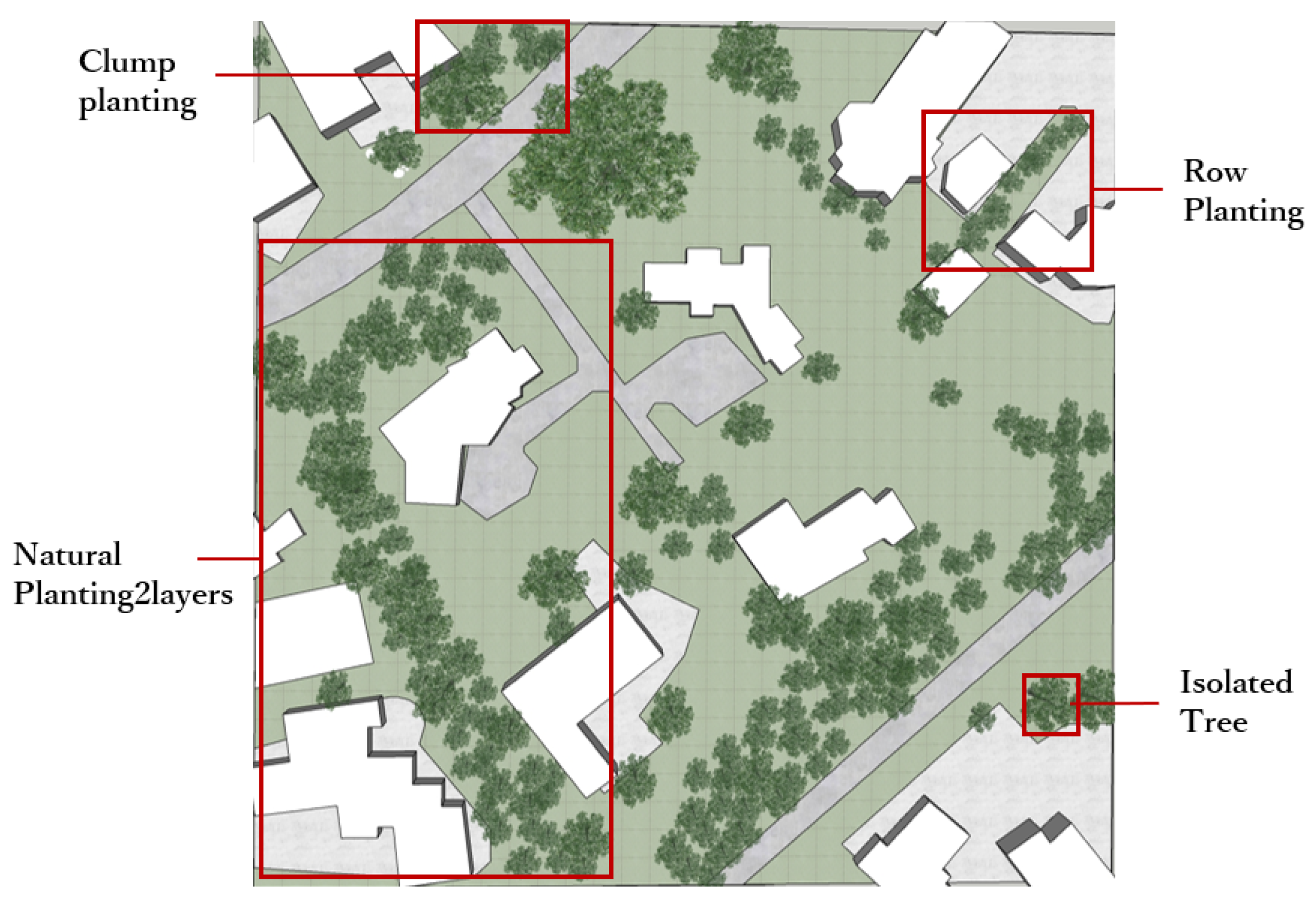
Our planting rules were inspired by the book Planting Design [13], encompassing a total of eight distinct planting arrangements. These arrangements cover both naturalistic and structured configurations. The eight planting arrangements are clump planting, row planting, open forest, scattered forest, belt planting, closed forest, nature planting 2layers, and mass planting. The distribution patterns can be referred to in Figure 5. Clump planting and row planting are common tree distribution patterns, so we consider them to be present in all regions. The other distribution patterns are specific to different regions.
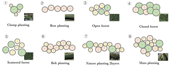
Figure 5.
Illustrations of different planting rules. We utilized a total of eight different planting rules. Under each rule, tree crown sizes vary. In the lower right corner of each planting rule, we show the corresponding real-world tree distribution for different rules. In this representation, we use green for larger crowns, red for medium-sized crowns, and yellow for smaller crowns. For further details, refer to Section 3.3.3. Our approach under these rules exhibits a more realistic representation of tree clusters.
Clump planting refers to a combination of one to ten trees with varying sizes, including both large trees and shrubs. It forms a highly naturalistic plant landscape. We apply the clump planting rule to those smaller clusters of trees with an area less than 2000 square units.
Row planting, belt planting, and nature planting 2layers are three types of strip planting rules, each with its own distinct characteristics. Row planting involves arranging trees of similar sizes in a single row to create a neat and uniform landscape. Belt planting, on the other hand, consists of 2 to 3 layers of trees, including main species, secondary species, or shrubs, with closely spaced trees. This type of planting can serve functions like windbreak and soil conservation, commonly seen in agricultural fields. Nature planting 2layers is a more complex tree landscaping method, involving a diverse selection of trees of varying sizes and heights, arranged in two layers to create a natural-looking planting arrangement. This type of planting is often used in well-landscaped residential areas. We differentiate these planting rules based on hyperparameters. Forests with values of p > 0.05 and r > 4 are identified as row planting. For forests that do not meet these criteria, those with p > 0.04 and r > 2.5 are assigned the remaining two rules in agricultural and residential areas, respectively.
Open forest, closed forest, and scattered forest are three planting rules based on tree density. In our approach, we assign these rules to grassland, agricultural areas, and industrial areas, respectively.
Mass planting is a larger-scale tree arrangement compared to the clump planting. Unlike clump planting, mass planting emphasizes overall aesthetics and can involve the use of the same or multiple tree species for combination. We apply this diverse planting rule to residential areas.
In the process of determining the planting rules for shrubs, we first confirm two common tree arrangements: clump planting and row planting. If the arrangement does not fall under these two categories, we proceed to determine whether it belongs to the other two types of strip planting arrangements. After excluding these four options, we then allocate the remaining planting rules based on different regions.
Finally, we determine the tree distribution within each vegetation cluster based on the chosen planting rules. We start by defining the lattice side length based on the tree crown radius baseline for the specific region where the vegetation cluster is located. This lattice side length is also influenced by the tree density coefficient associated with different planting rules. We use this lattice to partition the vegetation cluster polygon and randomly select points within the lattice cells’ central regions as the positions for the trees. If a selected center point falls outside the vegetation cluster polygon or is too close to the polygon’s edges, it is repositioned. Once the positions for each tree are determined, we calculate their tree crown radii based on the region’s tree crown radius baseline. The radius calculation is influenced by three main factors: a random fluctuation factor for the tree crown radius, a planting rule factor , and a boundary distance balance factor .
The factor represents the radius coefficient for different planting rules. For instance, under the mass planting rule, it could be chosen to represent a larger tree crown radius coefficient for the dominant tree species, or in the case of clump planting, a smaller tree crown radius coefficient for the complementary tree species. The factor is a radius coefficient that penalizes tree crown radii based on the proximity of the tree center to the edges of the vegetation cluster polygon. When the tree center is too close to the polygon’s edges, it leads to a reduction in the tree crown radius. This adjustment aims to decrease the potential error between the estimated tree distribution and the actual vegetation cluster configuration.
3.3.4. Height Estimation
Reconstructing tree height from a single optical image is a challenging task, which is why few attempts have been made to estimate tree height in previous work [10,27]. However, since we obtained the crown radius of each tree in the previous step, we can use this information as a basis for roughly estimating the tree height. We base our tree height estimation on the equation proposed by Hiernaux in their work [47]. The formula for height estimation is as follows:
where H represents the estimated tree height, and are equation parameters, stands for the crown area, and is an estimation error fluctuation value. We ultimately determined to be 1.8317 and to be 0.3936. After completing the height estimation for the trees, we acquired all the necessary information for reconstructing the three-dimensional urban tree landscape. This enables us to easily accomplish the task of tree modeling. Our height estimation evaluates the plausibility of tree heights under different planting strategies. Additionally, the 3D reconstruction visualization results demonstrate the diversity of tree heights.
4. Results
4.1. Experimental Setup
Our object detection neural network is built upon the MMDetection framework, while the semantic segmentation network is implemented using the Paddle framework. All methods are implemented in Python 3.8, and the results are saved in JSON files. The experiments were conducted on a machine equipped with a GeForce RTX 2070 SUPER GPU manufactured by NVIDIA Corporation (Santa Clara, CA, USA). For the object detection network, we employed the AdamW optimizer with a learning rate of 0.0002 and a weight decay of 0.0001. The maximum number of epochs was set to 100.
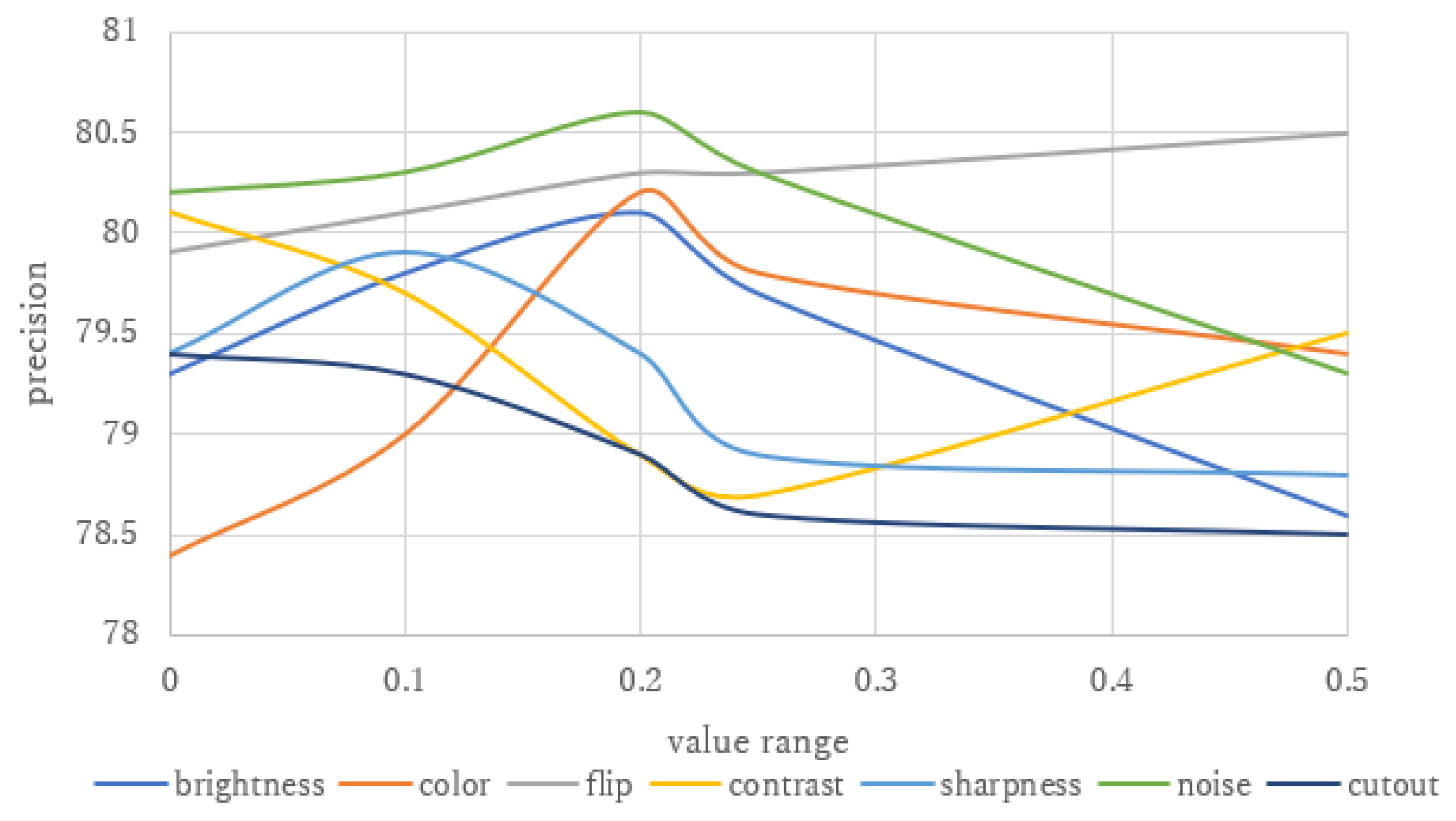
The training of the object detection network and semantic segmentation network is performed independently. The input for the object detection network is the annotated dataset, while the input for the semantic segmentation network is the cropped dense forest and shrub image patches from the annotated dataset. These image patches are resized to the same size and subjected to data augmentation to enhance the robustness of the network. We adjusted the brightness, saturation, flipping, contrast, clarity, noise, and occlusion, and refer to Figure 6 for the impact on accuracy. We ultimately chose not to use cutout; the ranges of clarity and contrast were set to 0.1, and the ranges of brightness and saturation were set to 0.2. The flipping probability was set to 0.4, and the Gaussian noise value was set to 20.
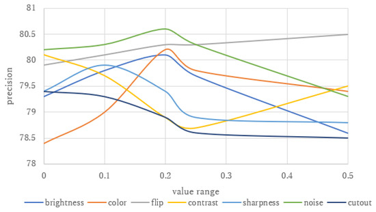
Figure 6.
Influence of different data augmentation methods on final loss. In this figure, we illustrate the impact of different data augmentation methods on the final loss. Too little data augmentation can result in insignificant effects, while excessive augmentation can deviate from real remote sensing images. Hence, most of the floating values are set closer to the median value to achieve optimal results.
4.2. Comparison of Detection Results
As we introduced the separation of single trees and complex tree clusters as two distinct objectives in the detection task, we chose to evaluate our method using popular object detection algorithms like Faster R-CNN [38] and DETR [29]. Despite the strong performance of these methods in common object detection tasks, they performed inadequately in our task due to their unique nature. Hence, this comparison was necessary, and we proceeded to analyze the reasons behind the poor performance. The aforementioned methods were all experimented on our dataset, and the quantitative comparison results are presented in Table 3. We compared the Average Precision and overall score for each category, as well as the time required for each method to detect trees. The scores before using NMS are shown in parentheses.

Table 3.
Quantitative comparison of detection results. This table provides a quantitative comparison of detection results using different object detection neural networks. Bold indicates the best-performing results. The values in parentheses indicate the results after applying Non-Maximum Suppression (NMS). We compare the Average Precision (AP) for three different tree categories to assess performance in different classes. Additionally, we compare the overall Average Precision (AP) and Average Recall (AR). The last column is a comparison of the detection time.
In comparisons with different methods, our approach achieved the best results in all the metrics. For the detection of low shrubs, where the training dataset was limited, the results were comparable among the four methods. However, for trees and tree clusters, using NMS led to a significant improvement in the results. In terms of detection time, our method is second best, slower by 1 s compared to the best method. All methods completed result generation within 20 to 30 s. This indicates that we can achieve optimal detection results while quickly completing the detection task. Visual comparisons of the detection results are shown in Figure 7.
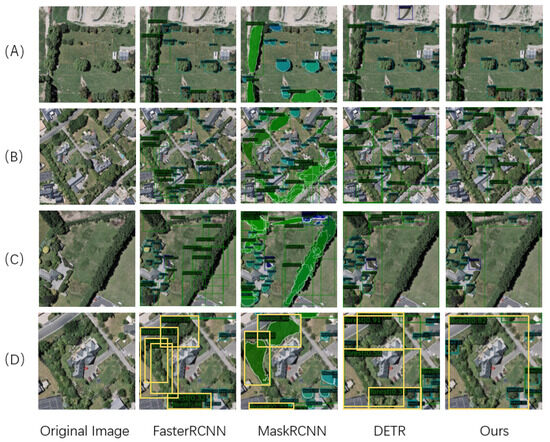
Figure 7.
Comparison of detection performance for different networks. In rows (A–C), you can see a comparison of the detection results for different networks. The leftmost column shows the original image, while the following columns display the detection results of various networks. Row (D) is an enlarged view of the top left part of row (B), with highlighted bounding boxes to better visualize the results. Our method reduces the issue of duplicate detections.
In the MaskRCNN and FasterRCNN methods, it is evident that when detecting large continuous clusters of vegetation, they tend to identify the same cluster as multiple objects, leading to errors. This phenomenon is challenging to reflect in the above score data. In Figure 7D, the Faster-RCNN method detects three consecutive dense forests on the left side (three yellow bounding boxes). This means that for one tree in that area, three trees will be generated at adjacent positions, which is not the desired result. We hope to generate only one tree for each tree. Our goal is to use a method that generates only one detection result for continuous dense forests. As shown in Figure 7D, only our method detects one result for continuous dense forests, while other methods detect overlapping multiple regions. Therefore, we believe that the Transformer-based method reduces the issue of repeated detections. This issue primarily arises because both of these methods are based on candidate regions (proposals). Before detecting the target, the model generates numerous candidate regions in the image and then identifies objects within these regions. When applied to vegetation cluster detection, it is understandable that regardless of whether a candidate region contains the largest enclosing box of a vegetation cluster, it will still be considered to be a region containing a cluster. This peculiarity arises due to the specific nature of our task, where even a portion of a cluster can still be considered a cluster. Figure 7D illustrates this point. We magnified the large vegetation cluster on the left side of Figure 7B and highlighted the detection results for this cluster. It is evident that MaskRCNN and FasterRCNN exhibit significant errors in this context. In contrast, the transformer-based method does not rely on proposals, which greatly reduces the occurrence of such repeated detections. DETR mainly encounters detection errors in localized regions as seen in Figure 7A, where it mistakenly identifies the grassland as a low shrub cluster. Our method performs well both globally and locally.
4.3. Single-Tree Detection
One of the significant features of our approach is that we distinguish individual trees from indistinct tree clusters. In previous works [12], not making this distinction often led to the misclassification of individual trees when using density-based methods. In our approach, we emphasize the correctness of individual tree detection, which contributes to a more realistic reconstruction of urban tree landscapes. Consequently, we introduce a new metric termed “Individual Tree Detection Accuracy”. For each image, we count the number of correctly predicted individual trees and compute both precision and recall, as shown in Table 4.

Table 4.
Table of accuracy in individual tree detection. Bold indicates the best-performing results.
Our method achieves an accuracy of 82.3% and a recall of 90.5% in individual tree detection, outperforming all other methods. We observe that the lower precision compared to recall is due to many trees within clusters being detected as individual trees. However, this phenomenon does not significantly affect the overall tree reconstruction. We also notice that DETR has particularly low precision, primarily because it often identifies the same tree as multiple objects. The NMS step in our method helps alleviate this issue.
4.4. The Impact of Planting Rules
To quantify the impact of the planting rules we proposed on tree distribution and tree height estimation, we introduced two metrics: a comparison between tree distributions applying rules versus random distribution in different regions, and the mean and standard deviation of tree heights under different rules.
In the first comparison, we set the control group’s tree distribution to use a random distribution, which is also the method used in [12]. When determining the size of the tree crown for the control group, we use the mean crown size of the region. We calculated the area of each segmented tree polygon as a reference value and measured the ratio of the sum of crown areas under the final tree distribution to the reference area. A ratio closer to 1 indicates a better fit with the original image, less than 1 suggests gaps or missing tree distribution, and greater than 1 suggests tree distribution with overflow or overlap. The comparison results are shown in Table 5.

Table 5.
Comparison of planting rules vs. random distribution in different regions. Bold indicates the best-performing results.
Our method achieved results closer to the ground truth in farmland, residential, and grassland, while it performed slightly worse in industrial areas. We also observed that, compared to random distribution, our method often generated smaller total canopy areas. Apart from the two fixed planting rules (clump planting and row planting), the varying planting rules we used in different regions contributed to these effects.
In farmland, we used belt planting and closed forest, which have higher tree density and typically larger trees, leading to larger canopy areas. In residential areas, we applied nature planting 2layers and clump planting since there are many small trees in residential areas. Therefore, we used a more conservative canopy radius coefficient in our method, resulting in smaller canopy areas. In grassland areas, we mainly used open forest, which has lower tree density. In industrial areas, we primarily used scattered forest, which might be the reason for the larger deviation between our distribution and the actual one. Furthermore, using ellipses to approximate trees can also lead to gaps. In contrast to squares, which can be tightly packed without leaving any spaces, ellipses are less compactly arranged, resulting in gaps between them, especially when there is no overlap between the ellipses.
It should be noted that in [12], the number of trees is only related to the area and contour of the region, which means that in the same region, regardless of the size of the tree crowns, the number of trees is the same. However, in reality, if the size of the tree crowns in a region is larger, there should be fewer trees compared to regions with smaller tree crowns. In this paper, since we took into account urban areas and forest characteristics (see Section 3.3.2 and Section 3.3.3 for details), and used planting rules, the distribution results are more diverse.
In the second metric, we calculated the mean and standard deviation of tree heights under different rules. This demonstrates that our method generates trees with varying heights, making our results more realistic compared to some previous works. The results are shown in Table 6. Additionally, we calculated the standard deviations for all isolated trees and the entire tree canopy as a reference. The standard deviation for isolated trees is 3.298 m, while for the entire tree canopy, it is 1.156 m. The reason for this difference is that in isolated trees, the canopy radii often vary significantly, leading to large differences in tree heights. In tree canopies, there are often large clusters of the same tree species; hence, we use a relatively conservative height estimation, resulting in less variation in tree heights. Specific differences in height estimation for each rule are provided in Table 6. The closed forest has the highest mean height, primarily because closed forests typically consist of tall and large deciduous trees. The closed forest also has the smallest standard deviation, resulting in a dense and uniform appearance from the outside. Similarly, row planting has a small standard deviation due to our method making them appear as the same tree type from the outside. On the other hand, we observed that clump planting has the largest standard deviation in height. This is because clump planting areas are smaller and may contain multiple tree species, leading to significant height variations among them. Additionally, we found that the trees in the scattered forest rule tend to be shorter on average. This might be due to the fact that the scattered forest areas, mainly in industrial zones, have shorter trees. Through this metric, our method demonstrates the diversity of tree heights and maintains realism under different planting rules.

Table 6.
Mean and standard deviation of tree heights under different rules.
4.5. Visualization Results
After obtaining the urban tree information, we saved it in JSON files. These data can be easily accessed and used for urban three-dimensional reconstruction. We conducted three-dimensional visualization reconstruction of the obtained results using SketchUp 2023. Even newcomers without any modeling experience can easily achieve the three-dimensional reconstruction of urban vegetation.
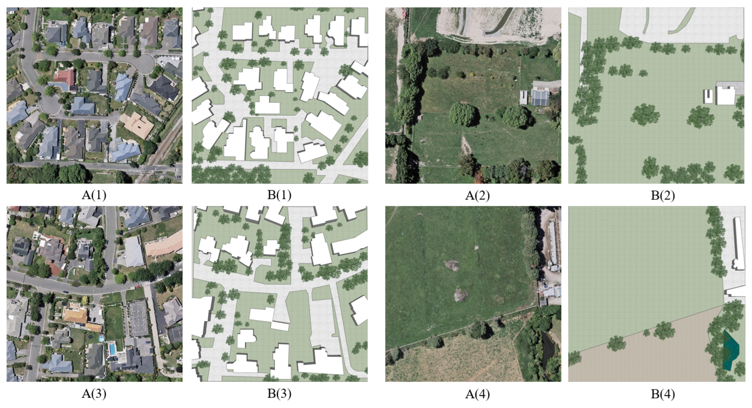
Figure 8 shows the reconstruction results for four different images. Our method accurately reproduces the positions and sizes of isolated trees. For large tree clusters, our method provides a simulation of tree distribution that closely resembles the original image.

Figure 8.
The 3D reconstruction results for different images. In this figure, you can observe the 3D reconstruction results for various images. (A(1)) and (A(3)) represent residential areas, while (A(2)) and (A(4)) correspond to farmland. (B(1))–(B(4)) show the respective 3D reconstruction results.
In Figure 9, we showcase the effects of various planting rules applied to the reconstructed images. Apart from isolated trees, we applied rules like clump planting, row planting, and nature planting 2layers to complex forest environments in the images.
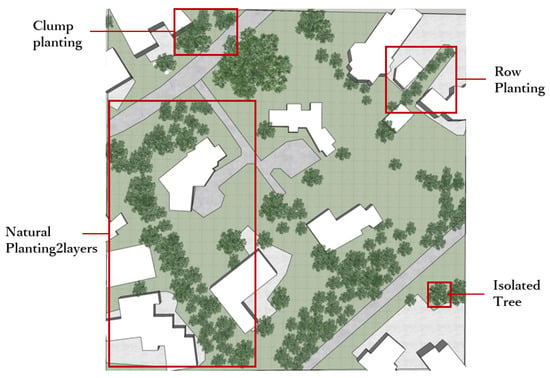
Figure 9.
Effects of different planting rules applied in 3D reconstruction. In this figure, we illustrate the effects of different planting rules applied in 3D reconstruction. We utilized clump planting, row planting, and natural planting 2layers for this demonstration.
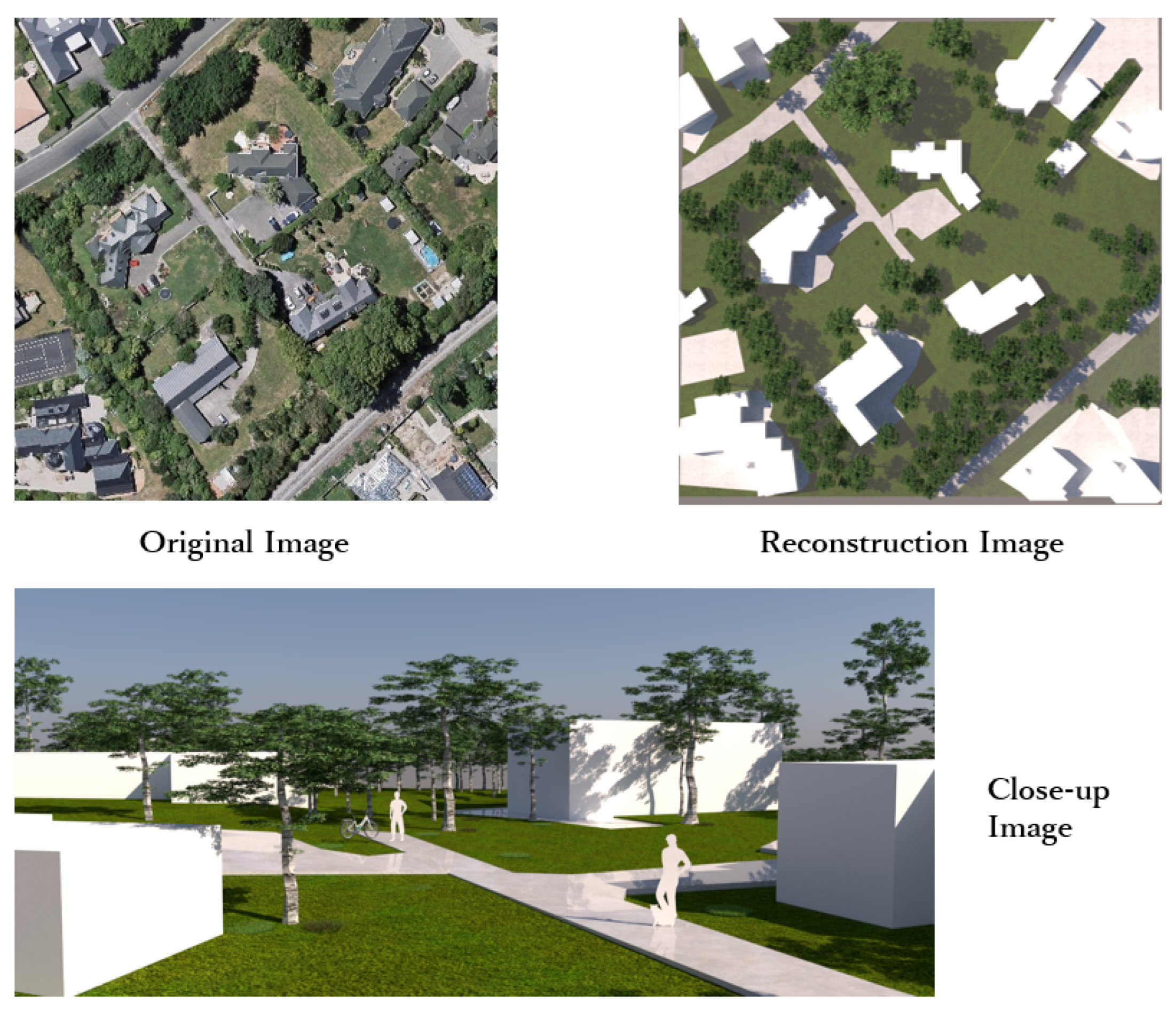
In Figure 10, we display the rendered reconstruction results and close-up images. Compared to previous tree generation methods, our approach, which leverages information about tree positions, crown sizes, heights, and more, creates a more realistic representation of urban trees. Additionally, our method offers a wider variety of tree combinations, resulting in more natural urban tree modeling.
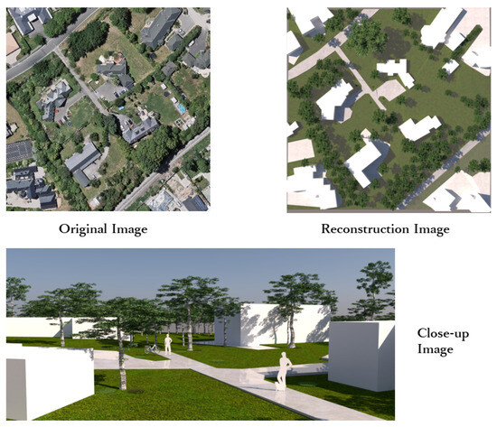
Figure 10.
Original images and rendered 3D reconstruction results. In this figure, we showcase the original images and the rendered results of our 3D reconstruction. After rendering, our reconstruction results effectively capture the tree environment from the original images. In the close-up view below, you can observe the realistic arrangement of our trees.
5. Discussion
Our current method combines neural networks and procedural generation to provide a superior solution for 3D reconstruction of trees from real images. By incorporating an object detection network instead of solely relying on semantic segmentation, we achieve an accuracy of 82.3% for single tree detection. Additionally, we propose treating continuous dense forests as individual tree units and using them as one of the classification targets in object detection. This helps eliminate the ambiguity issues faced by [10], who labeled dense forests as a group and ended up segmenting multiple tree crowns, leading to decreased evaluation accuracy. Our single-tree detection accuracy surpasses their method’s 70.9% accuracy because our approach avoids interference from dense forests. Compared to the method proposed by Firoze et al. [12], our method does not require additional synthetic data and avoids misclassifying large, isolated trees as multiple trees. Furthermore, our method automatically segments the input image into different regions, eliminating the need for manual segmentation. Additionally, when generating the tree distribution, our method uses various planting rules, making our tree distribution more realistic.
Our method still has some limitations and areas for improvement. Firstly, although we used the latest object detection network, deformable DETR [40], we did not make significant architectural changes to adapt it to the task of tree detection in remote sensing images. Therefore, there is room for improvement in detection performance in future work. Additionally, since we use two neural networks, errors in detection can propagate and lead to errors in semantic segmentation. While we mitigated such errors through data preprocessing, there may still be some unavoidable mistakes. In future work, optimizing the networks can help reduce these types of errors. Furthermore, in simulating trees in the forest using planting rules, our method, like some previous works, has a limitation. When splitting a forest into multiple trees to maintain separation between them, it can lead to gaps in the overall forest. This becomes more apparent when we perform three-dimensional reconstruction on remote sensing images. In future work, adjustments to the planting rules will be needed to reduce the occurrence of these gaps. Additionally, we will incorporate the consideration of tree shadows to improve our ability to make more accurate estimations of the heights of taller trees. As this paper uses a dataset of single optical images without ortho-correction, we will consider the impact of ortho-correction on single optical remote sensing images in future work.
6. Conclusions
We propose an urban tree distribution generation method that combines target detection methods with procedural generation based on planting rules for the reconstruction of complex urban trees. We propose breaking down the problem of tree localization into two parts—individual trees and dense forests—and taking into account the impact of urban regional attributes and crown size on tree distribution. First, we improve the accuracy of individual tree detection by introducing target detection algorithms to handle the dominant individual trees and combining semantic segmentation to process dense forests. Then, we optimize the tree distribution results by designing a tree distribution generation algorithm based on planting rules, making the generated results more similar to the real distribution. Additionally, this method is insensitive to whether the crown boundaries are blurry. Finally, our results can be directly used for the 3D reconstruction visualization of urban trees.
Author Contributions
Conceptualization, Q.S.; Methodology, H.G., R.S. and C.F.; Software, H.G. and R.S.; Investigation, H.G., C.F., R.S. and Q.S.; Resources, R.S., Q.S. and L.S.; Writing—original draft, H.G., Q.S. and C.F.; Writing—review and editing, H.G. and Q.S.; Visualization, H.G. and C.F.; Supervision, R.S. and Q.S.; Funding acquisition, R.S. and Q.S. All authors have read and agreed to the published version of the manuscript.
Funding
This work was supported by the National Natural Science Foundation of China under Grant 61702363, and Grant 62222311, the Startup Foundation for Introducing Talent of NUIST 2022r075.
Data Availability Statement
The data used to support the findings of this study are available from the corresponding author upon request.
Conflicts of Interest
The authors declare no conflicts of interest.
References
- Global Forest Resources Assessment 2020—Key Findings. Available online: https://doi.org/10.4060/ca8753en (accessed on 21 July 2020).
- Guldin, R.W. Forest science and forest policy in the Americas: Building bridges to a sustainable future. For. Policy Econ. 2003, 5, 329–337. [Google Scholar] [CrossRef]
- Cao, S.; Sun, G.; Zhang, Z. Greening China naturally. Ambio 2011, 40, 828–831. [Google Scholar] [CrossRef]
- Oldfield, E.E.; Felson, A.J.; Auyeung, D.S.N.; Crowther, T.W.; Sonti, N.F.; Harada, Y.; Maynard, D.S.; Sokol, N.W.; Ashton, M.S.; Warren, R.J., II; et al. Growing the urban forest: Tree performance in response to biotic and abiotic land management. Restor. Ecol. 2015, 23, 707–718. [Google Scholar] [CrossRef]
- Turner, W.; Rondinini, C.; Pettorelli, N.; Mora, B.; Leidner, A.K.; Szantoi, Z.; Buchanan, G.; Dech, S.; Dwyer, J.; Herold, M.; et al. Free and open-access satellite data are key to biodiversity conservation. Biol. Conserv. 2015, 182, 173–176. [Google Scholar] [CrossRef]
- Hansen, M.C.; Potapov, P.V.; Moore, R.; Hancher, M.; Turubanova, S.A.; Tyukavina, A.; Thau, D.; Stehman, S.V.; Goetz, S.J.; Loveland, T.R.; et al. High-resolution global maps of 21st-century forest cover change. Science 2013, 342, 850–853. [Google Scholar] [CrossRef] [PubMed]
- Fox, J.C.; Ades, P.K.; Bi, H. Stochastic structure and individual-tree growth models. For. Ecol. Manag. 2001, 154, 261–276. [Google Scholar] [CrossRef]
- Rohner, B.; Waldner, P.; Lischke, H.; Ferretti, M.; Thürig, E. Predicting individual-tree growth of central European tree species as a function of site, stand, management, nutrient, and climate effects. Eur. J. For. Res. 2018, 137, 29–44. [Google Scholar] [CrossRef]
- Brandt, M.; Tucker, C.J.; Kariryaa, A.; Rasmussen, K.; Abel, C.; Small, J.; Chave, J.; Rasmussen, L.V.; Hiernaux, P.; Diouf, A.A.; et al. An unexpectedly large count of trees in the West African Sahara and Sahel. Nature 2020, 587, 78–82. [Google Scholar] [CrossRef]
- Freudenberg, M.; Magdon, P.; Nölke, N. Individual tree crown delineation in high-resolution remote sensing images based on U-Net. Neural Comput. Appl. 2022, 34, 22197–22207. [Google Scholar] [CrossRef]
- Niese, T.; Pirk, S.; Albrecht, M.; Benes, B.; Deussen, O. Procedural Urban Forestry. ACM Trans. Graph. 2022, 41, 1–18. [Google Scholar] [CrossRef]
- Firoze, A.; Benes, B.; Aliaga, D. Urban tree generator: Spatio-temporal and generative deep learning for urban tree localization and modeling. Vis. Comput. 2022, 38, 3327–3339. [Google Scholar] [CrossRef]
- Lu, J. Planting Design, 1st ed.; China Architecture & Building Press: Beijing, China, 2008; pp. 62–87. [Google Scholar]
- Crowther, T.W.; Glick, H.B.; Covey, K.R.; Bettigole, C.; Maynard, D.S.; Thomas, S.M.; Smith, J.R.; Hintler, G.; Duguid, M.C.; Amatulli, G.; et al. Mapping tree density at a global scale. Nature 2015, 525, 201–205. [Google Scholar] [CrossRef]
- Nowak, D.J.; Crane, D.E.; Stevens, J.C.; Hoehn, R.E.; Walton, J.T.; Bond, J. A ground-based method of assessing urban forest structure and ecosystem services. Arboric. Urban For. 2008, 34, 347–358. [Google Scholar] [CrossRef]
- Edson, C.; Wing, M.G. Airborne Light Detection and Ranging (LiDAR) for individual tree stem location, height, and biomass measurements. Remote Sens. 2011, 3, 2494–2528. [Google Scholar] [CrossRef]
- Wang, L. A Multi-scale Approach for Delineating Individual Tree Crowns with Very High Resolution Imagery. Photogramm. Eng. Remote Sens. 2010, 76, 371–378. [Google Scholar] [CrossRef]
- Martins, J.; Junior, J.M.; Menezes, G.; Pistori, H.; Sant, D.; Gonçalves, W. Image Segmentation and Classification with SLIC Superpixel and Convolutional Neural Network in Forest Context. In Proceedings of the IGARSS 2019—2019 IEEE International Geoscience and Remote Sensing Symposium, Yokohama, Japan, 28 July 2019. [Google Scholar]
- Culvenor, D.S. TIDA: An algorithm for the delineation of tree crowns in high spatial resolution remotely sensed imagery. Comput. Geosci. 2002, 28, 33–44. [Google Scholar] [CrossRef]
- Ghasemi, M.; Latifi, H.; Pourhashemi, M. A Novel Method for Detecting and Delineating Coppice Trees in UAV Images to Monitor Tree Decline. Remote Sens. 2022, 14, 5910. [Google Scholar] [CrossRef]
- Sivanandam, P.; Lucieer, A. Tree Detection and Species Classification in a Mixed Species Forest Using Unoccupied Aircraft System (UAS) RGB and Multispectral Imagery. Remote Sens. 2022, 14, 4963. [Google Scholar] [CrossRef]
- Onishi, M.; Ise, T. Explainable identification and mapping of trees using UAV RGB image and deep learning. Sci. Rep. 2021, 11, 903. [Google Scholar] [CrossRef]
- Firoze, A.; Wingren, C.; Yeh, R.A.; Benes, B.; Aliaga, D. Tree Instance Segmentation with Temporal Contour Graph. In Proceedings of the IEEE/CVF Conference on Computer Vision and Pattern Recognition, Vancouver, BC, Canada, 17–24 June 2023. [Google Scholar]
- Guo, J.; Xu, Q.; Zeng, Y.; Liu, Z.; Zhu, X.X. Nationwide urban tree canopy mapping and coverage assessment in Brazil from high-resolution remote sensing images using deep learning. ISPRS J. Photogramm. Remote Sens. 2023, 198, 1–15. [Google Scholar] [CrossRef]
- Liu, T.; Yao, L.; Qin, J.; Lu, J.; Lu, N.; Zhou, C. A Deep Neural Network for the Estimation of Tree Density Based on High-Spatial Resolution Image. IEEE Trans. Geosci. Remote Sens. 2021, 60, 4403811. [Google Scholar] [CrossRef]
- Li, S.; Brandt, M.; Fensholt, R.; Kariryaa, A.; Igel, C.; Gieseke, F.; Nord-Larsen, T.; Oehmcke, S.; Carlsen, A.H.; Junttila, S.; et al. Deep learning enables image-based tree counting, crown segmentation, and height prediction at national scale. PNAS Nexus 2023, 2, 76. [Google Scholar] [CrossRef] [PubMed]
- Yang, M.; Mou, Y.; Liu, S.; Yanrong, M.; Zelin, L.; Peng, L.; Wenhua, X.; Xiaolu, Z.; Changhui, P. Detecting and mapping tree crowns based on convolutional neural network and Google Earth images. Int. J. Appl. Earth Obs. Geoinf. 2022, 108, 102764. [Google Scholar] [CrossRef]
- Liu, Z.; Lin, Y.; Cao, Y.; Hu, H.; Wei, Y.; Zhang, Z.; Lin, S.; Guo, B. Swin Transformer: Hierarchical Vision Transformer using Shifted Windows. In Proceedings of the IEEE/CVF International Conference on Computer Vision, Montreal, QC, Canada, 25 March 2021. [Google Scholar]
- Carion, N.; Massa, F.; Synnaeve, G.; Usunier, N.; Kirillov, A.; Zagoruyko, S. End-to-End Object Detection with Transformers. In Proceedings of the European Conference on Computer Vision, Glasgow, UK, 23 August 2020. [Google Scholar]
- Demir, I.; Aliaga, D.G.; Benes, B. Proceduralization of buildings at city scale. In Proceedings of the 2014 2nd International Conference on 3D Vision, Washington, DC, USA, 8–11 December 2014. [Google Scholar]
- Kelly, T.; Femiani, J.; Wonka, P.; Mitra, N.J. BigSUR: Large-scale structured urban reconstruction. ACM Trans. Graph. 2017, 36, 204. [Google Scholar] [CrossRef]
- Roglà, P.O.; Pelechano, G.N.; Patow, G.A. Procedural semantic cities. In Proceedings of the CEIG 2017: XXVII Spanish Computer Graphics Conference, Sevilla, Spain, 28–30 June 2017. [Google Scholar]
- Beneš, B.; Massih, M.A.; Jarvis, P.; Aliaga, D.G.; Vanegas, C.A. Urban ecosystem design. In Proceedings of the Symposium on Interactive 3D Graphics and Games, San Francisco, CA, USA, 18–20 February 2011. [Google Scholar]
- Benes, B.; Zhou, X.; Chang, P.; Cani, M.P.R. Urban Brush: Intuitive and Controllable Urban Layout Editing. In Proceedings of the 34th Annual ACM Symposium on User Interface Software and Technology, New York, NY, USA, 10 October 2021. [Google Scholar]
- Hao, Z.; Lin, L.; Post, C.J.; Yu, K.; Liu, J.; Lin, L.; Chen, Y.; Mikhailova, E.A. Automated tree-crown and height detection in a young forest plantation using mask region-based convolutional neural network (Mask R-CNN). ISPRS J. Photogramm. Remote Sens. 2021, 178, 112–123. [Google Scholar] [CrossRef]
- Guirado, E.; Blanco-Sacristan, J.; Rodriguez-Caballero, E.; Tabik, S.; Alcaraz-Segura, D.; Martínez-Valderrama, J.; Cabello, J. Mask R-CNN and OBIA fusion improves the segmentation of scattered vegetation in very high-resolution optical sensors. Sensors 2021, 21, 320. [Google Scholar] [CrossRef] [PubMed]
- Blum, J. Urban Forests: Ecosystem Services and Management, 1st ed.; Apple Academic Press: New York, NY, USA, 2017; pp. 234–236. [Google Scholar]
- Ren, S.; He, K.; Girshick, R.; Sun, J. Faster r-cnn: Towards real-time object detection with region proposal networks. Adv. Neural Inf. Process. Syst. 2015, 28, 1–9. [Google Scholar] [CrossRef] [PubMed]
- Vaswani, A.; Shazeer, N.; Parmar, N.; Uszkoreit, J.; Jones, L.; Gomez, A.N.; Kaiser, Ł.; Polosukhin, I. Attention is all you need. Adv. Neural Inf. Process. Syst. 2017, 30, 1–11. [Google Scholar]
- Zhu, X.; Su, W.; Lu, L.; Li, B.; Wang, X.; Dai, J. Deformable detr: Deformable transformers for end-to-end object detection. arXiv 2020, arXiv:2010.04159. [Google Scholar]
- He, K.; Zhang, X.; Ren, S.; Sun, J. Deep residual learning for image recognition. In Proceedings of the 2016 IEEE Conference on Computer Vision and Pattern Recognition (CVPR), Las Vegas, NV, USA, 27–30 June 2016. [Google Scholar]
- Lin, T.Y.; Goyal, P.; Girshick, R.; He, K.; Dollár, P. Focal loss for dense object detection. In Proceedings of the 2017 IEEE International Conference on Computer Vision (ICCV), Venice, Italy, 22–29 October 2017. [Google Scholar]
- Neubeck, A.; Van Gool, L. Efficient non-maximum suppression. In Proceedings of the 18th International Conference on Pattern Recognition (ICPR’06), Hong Kong, China, 20–24 August 2006. [Google Scholar]
- Huang, H.; Lin, L.; Tong, R.; Hu, H.; Zhang, Q.; Iwamoto, Y.; Han, X.; Chen, Y.W.; Wu, J. Unet 3+: A full-scale connected unet for medical image segmentation. In Proceedings of the ICASSP 2020–2020 IEEE International Conference on Acoustics, Speech and Signal Processing (ICASSP), Barcelona, Spain, 4–8 May 2020. [Google Scholar]
- Ronneberger, O.; Fischer, P.; Brox, T. U-net: Convolutional networks for biomedical image segmentation. In Proceedings of the Medical Image Computing and Computer-Assisted Intervention—MICCAI 2015: 18th International Conference, Munich, Germany, 5–9 October 2015. [Google Scholar]
- Bourne, K.S.; Conway, T.M. The influence of land use type and municipal context on urban tree species diversity. Urban Ecosyst. 2014, 17, 329–348. [Google Scholar] [CrossRef]
- Hiernaux, P.; Issoufou, H.B.A.; Igel, C.; Kariryaa, A.; Kourouma, M.; Chave, J.; Mougin, E.; Savadogo, P. Allometric equations to estimate the dry mass of Sahel woody plants mapped with very-high resolution satellite imagery. For. Ecol. Manag. 2023, 529, 120653. [Google Scholar] [CrossRef]
Disclaimer/Publisher’s Note: The statements, opinions and data contained in all publications are solely those of the individual author(s) and contributor(s) and not of MDPI and/or the editor(s). MDPI and/or the editor(s) disclaim responsibility for any injury to people or property resulting from any ideas, methods, instructions or products referred to in the content. |
© 2024 by the authors. Licensee MDPI, Basel, Switzerland. This article is an open access article distributed under the terms and conditions of the Creative Commons Attribution (CC BY) license (https://creativecommons.org/licenses/by/4.0/).

