Article

Assessment Accuracy of Standard Point Positioning Enhanced by Observation and Position Domain Filtering Utilizing a Multi-Epoch Least-Squares Integration Method

1
College of Forestry (Academy of Forestry), Northwest A&F University, Yangling 712100, China
2
School of Environment Science and Spatial Informatics, China University of Mining and Technology, Xuzhou 221116, China
3
Nottingham Geospatial Institute, The University of Nottingham, Nottingham NG7 2TU, UK
4
Power China Northwest Engineering Corporation Limited, Xi’an 710065, China
5
Shaanxi Union Research Center of University and Enterprise for River and Lake Ecosystems Protection and Restoration, Xi’an 710065, China
6
Faculty of Architecture, Civil and Transportation Engineering, Beijing University of Technology, Beijing 100124, China
*
Author to whom correspondence should be addressed.
Remote Sens. 2024, 16(3), 517; https://doi.org/10.3390/rs16030517
Submission received: 28 December 2023 / Revised: 24 January 2024 / Accepted: 25 January 2024 / Published: 29 January 2024
(This article belongs to the Section Engineering Remote Sensing)

Abstract

:
To enhance the positioning accuracy of standalone GNSS receivers in environments unable to provide precise ephemeris and clock offset, such as undeveloped forest areas that lack network communication and power supply, this study employed the Time Difference Carrier Phase (TDCP) technology to improve the positioning accuracy of Standard Point Positioning (SPP), where the Least-Squares (LS) and the extended Multi-Epoch Least Squares (MELS) method were applied in the position domain filtering for a single GNSS receiver and compare its performance with the existing observation domain filtering method. Firstly, the simulated data sets with various positioning accuracies were used to verify the effectiveness and convergence of the LS filtering methods. The results indicate that the LS filtering method produces a lower root mean square (RMS) error than the original strategy. Secondly, this study uses two kinematic GNSS data sets to evaluate the performance of the observation and position domain filtering, with an emphasis on the MELS method. The numerical experiment results show that the position domain LS filtering method outperforms the other two methods. The open environment experiments result shows that the positioning domain filtering method achieved positioning accuracies of 0.202 m, 0.843 m, and 2.036 m in the E, N, and U directions, respectively, with improvements of 68.0%, 21.6%, and 24.0%, compared to the original algorithm which achieved positioning accuracies of 0.631 m, 1.076 m, and 2.680 m. It also achieved improvements of 24.0%, 4.0%, and 18.3%, respectively, compared to the observation domain filtering method with positioning accuracies of 0.353 m, 0.886 m, and 2.526 m. The forest scenes experiments result shows that the positioning domain filtering method achieved positioning accuracies of 1.308 m, 1.375 m, and 2.133 m in the E, N, and U directions, respectively, with improvements of 42.4%, 36.2%, and 27.6%, compared to original algorithm which achieved positioning accuracies of 1.863 m, 1.873 m, and 2.722 m, and also achieved improvements of 27.0%, 19.4% and 10.6%, respectively, comparing to observation domain filtering method with positioning accuracies of 1.661 m, 1.642 m and 2.359 m. Moreover, the examination of the LS method results based on different epochs reveals that the filtering accuracy increases as more epochs are incorporated into the position domain integration and the enhancement value reaches a few millimeters.

1. Introduction

Global Navigation Satellite System (GNSS) is a technology that uses satellite signals to provide Navigation, Positioning, and Timing (PNT) services, comprising the Global Position System (GPS), Global’naya Navigatsionnaya Sput-nikovaya Sistema (GLONASS), BeiDou Navigation Satellite System (BDS), and Galileo satellite navigation system (Galileo). GNSS has a wide range of applications in forestry, such as forest resource inventory, forest fire emergency, wildlife protection, etc. However, the positioning accuracy of GNSS is affected by various factors, such as the number and geometry of satellites, atmospheric delay, multipath effect, occlusion, etc. These factors are more severe in forest environments, leading to lower positioning accuracy of GNSS, which impedes the development of smart forestry [1]. Smart forestry is a mode that uses information technology and data analysis to achieve intelligent, refined, and efficient forest management. The core of smart forestry is information service based on spatial location, and GNSS is the main tool to provide spatial location information. Therefore, the positioning accuracy of GNSS directly influences the service quality and level of smart forestry. For example, in forest resource inventory, the positioning accuracy of GNSS determines the accuracy of plot location and relocation, which affects the estimation and evaluation of forest resources [2]; in forest fire emergency, the positioning accuracy of GNSS affects the location and analysis of fire scene, which affects the efficiency and outcome of firefighting [3]; in wildlife protection, the positioning accuracy of GNSS affects the tracking and monitoring of animals, which affects the protection strategies and measures [4]. A study has analyzed the positioning accuracy of using GNSS technology for kinematic positioning under different canopy closure levels, and the results show that due to the low sensitivity of single-frequency GNSS receivers, their accuracy is not affected much by forest conditions, while the accuracy of dual-frequency GNSS receivers is highly dependent on satellite visibility [5]. In addition, the literature first applied the Precise Point Positioning (PPP) Ambiguity Resolution (AR) technique to precise positioning in forest areas and studied the effects of canopy closure, observation time, and system combination on positioning accuracy [6].
The demand for high-precision positioning of smart forestry is driven by the business needs of forestry resources, forestry production, and forestry ecology and is an important technical support for the development of smart forestry. Also, high-precision positioning plays an important role in smart forestry, as it can not only improve the efficiency of monitoring and managing forestry resources but also provide accurate data support for forest management decision-making and promote the high-quality development of forestry. However, GNSS PNT services face significant challenges, mainly due to the limitations of the principles and functions of GNSS technology, resulting in the positioning solution of Single Point Positioning (SPP) and Precise Point Positioning (PPP). The low precision of SPP often leads to less accurate location data, thus reducing the usefulness of GNSS for critical applications. Moreover, the adoption of PPP as an alternative, more precise, and accurate positioning solution is hindered by the long convergence time, making it unsuitable for real-time applications [7]. In recent decades, several studies have been conducted to improve GNSS performance through a range of innovative methodologies. These methodologies focus on error mitigation of GNSS technology based on the following approaches: Satellite-Based Augmentation Systems (SBAS) and Ground-Based Augmentation Systems (GBAS) have emerged as effective strategies to correct GNSS errors. SBAS uses additional ground infrastructure and control centers to correct signal distortions from satellites, thus enhancing precision and reliability. On the other hand, GBAS improves positioning accuracy near airports, supporting aviation applications. Map-Matching Algorithms [8]: map-matching algorithms have gained popularity by integrating GNSS data with cartographic information to improve positional accuracy, which is suitable for applications such as vehicular navigation and autonomous driving, where precise location determination is required in urban environments with signal obstructions and strong multipath effects. Inertial Augmentation of GNSS [9]: the integration of Inertial Measurement Units (IMUs) with GNSS data has been applied as a robust positioning solution, where IMUs can capture acceleration and orientation data, mitigating the GNSS signal disruptions and multipath effects resulting in precise and high-rate positioning solution. PPP service [10]: PPP is based on the principle of exploiting ancillary satellite data and information to enhance GNSS accuracy. Although PPP solutions require long initialization periods, PPP achieves high precision and robust performances, and it is widely adopted in high-accuracy applications such as geolocation, agriculture, geodesy, and geophysics. However, it should be noted that all of these methodologies often require additional hardware components, such as base stations, data streams, and IMUs, which generate extra requirements and needs for the reliable and robust operation of the system, warranting careful consideration in deployment scenarios. The prospects of GNSS technology and applications are even more promising thanks to the advancements of multi-frequency high-rate GNSS receivers even for consumer-grade GNSS receivers, developments of communication technologies such as 5G, and an increased focus on cybersecurity and resilience, all of which create favorable conditions for precise and robust GNSS PNT performance.
Since most of the undeveloped forest areas lack network communication, this study addresses the needs of forest resource development in these areas and strives to enhance the positioning accuracy of GNSS without additional equipment to facilitate the development of smart forestry. Generally, filtering methods in the field of GNSS technology can be classified into two main domains: observation domain filtering methods and position domain filtering methods [11,12]. The observation domain filtering methods exploit the inherent characteristics of GNSS measurements, focusing on the unambiguous nature of pseudorange measurements and the high precision achieved by carrier phase measurements. A pioneering study in this field was conducted by Hatch, who introduced the concept of a carrier-smoothing pseudorange strategy [13]. This innovative approach is based on the fact that the theoretical change in pseudorange equals the corresponding carrier phase value. Over the years, this strategy has been refined and optimized to account for various factors, such as the effects of ionospheric variations, the challenges posed by multipath interference, the optimal smoothing window sizes, and the correlation information between current and previous observations [14,15,16,17,18]. Parameter estimation techniques have been developed to reduce the noise in distance measurements by integrating pseudorange and carrier phase. McGraw introduced the Generalized Divergence-Free Smoothing (GDFS) framework, offering a systematic approach for generating values with minimal pseudorange errors, facilitating the derivation of ionosphere-free measurements, and aiding in the resolution of integer ambiguities [19]. Direct positioning approaches based on maximum likelihood estimation have also been explored, with Closas et al. making notable contributions in this field [20,21]. However, this approach often requires substantial computational complexity, which can pose challenges, especially in real-time applications. Vincent et al. established the theoretical potential of integrating Doppler and pseudorange measurements to yield asymptotically accurate positioning results [22]. Nonetheless, this algorithm has mainly been tested in simulated environments, revealing the need for realistic, experimental validation. Qian et al. introduced a least-squares (LS) filtering method for integrating pseudorange and carrier phase observations, with primary validation conducted using simulated datasets, thereby warranting further empirical evaluation [23]. An enhanced version of the LS filtering method has been proposed by Li et al., who extended it from double-epochs to multi-epochs. Their comparative analysis, considering various smoothing window sizes and benchmarked against Hatch’s approach, provides valuable insights into the strengths and limitations of these techniques [24]. Moving to the position domain, a key challenge lies in establishing an accurate and suitable kinematic model to characterize the kinematic behavior of mobile GNSS receivers. Conventional models, such as the constant velocity (CV) and constant acceleration (CA) models, have been widely adopted but may not be universally suitable, especially when the carrier motion exhibits nonlinearity or varying sampling intervals [25]. In response to these limitations, alternative models have emerged, such as the differential polynomial model, Singer model, semi-Markov model, current statistical model, semi-Markov jump process model, and Markov acceleration model, which are better suited for capturing the kinematics of time-varying systems [26,27,28,29,30]. However, it should be noted that these models often require the spectral density matrix of navigation information, demanding constant updates as the carrier’s trajectory evolves [31]. Predictive models may not perform well in applications with irregular carrier movement, which highlights the importance of developing a state equation based on velocity measurements such as Doppler or Time Difference Carrier Phase (TDCP). Although LS filtering has proven effective in the observation domain, there is still a strong demand for further evaluation of filtering methods in the position domain [23]. Such empirical studies, carried out in various GNSS navigation scenarios, will greatly advance the ongoing effort to improve GNSS positioning accuracy and reliability, addressing the real-world challenges and variations in practical applications.
The filtering method of precision positioning technology currently used in smart forestry mainly inherits traditional GNSS positioning domain technology, including two main filtering methodologies: position domain filtering and observation domain filtering [32,33,34]. These filtering methods are essential for GNSS positioning, as they enable accurate and reliable location determination. Position domain filtering methods, such as the Kalman filter, are praised for their ability to provide high-precision location estimates with remarkable stability [35,36]. This makes them especially suitable for applications that require the fusion of data from multiple sensors, as they can smoothly integrate different data sources to produce a comprehensive position solution. However, the effectiveness of position domain filtering methods depends on the careful definition of the system’s dynamic model. This requires an accurate representation of the underlying physical processes that govern the GNSS receiver’s movement [37]. Therefore, position domain filtering methods may not be the best choice for applications with nonlinearities, as these methods usually perform poorly when the system dynamics are not well-modeled [38,39]. On the other hand, observation domain filtering methods, exemplified by the Least Squares (LS) approach, are known for their computational simplicity and speed, making them ideal for fast positioning scenarios [40]. They are particularly useful for applications where real-time or near-real-time positioning is crucial, such as in vehicular navigation or pedestrian tracking [41]. However, the drawback of observation domain filtering methods is their inherent sensitivity to signal quality and visibility constraints. These methods often have difficulty maintaining their accuracy in environments with signal multipaths, obstructions, or adverse atmospheric conditions [42]. The advantages of position domain filtering include not only high precision and stability but also the ability to integrate diverse data sources effectively [40]. This is particularly valuable in applications where redundancy and robustness are essential. However, this comes at the expense of increased computational complexity, as these methods involve the estimation of multiple parameters simultaneously. Moreover, the need for an accurate dynamic model can be a limiting factor in dynamic or nonlinear scenarios [43]. Conversely, observation domain filtering methods, with their computational simplicity, are well-suited for applications with limited computational resources. They can often provide satisfactory positioning accuracy in scenarios where signal quality is high and visibility is clear [43,44]. Nonetheless, their sensitivity to signal quality issues and the lack of consideration for dynamic models limit their usefulness in scenarios that require high precision or encounter dynamic movement [40,45]. In summary, the selection of an appropriate filtering method depends on a careful evaluation of the specific requirements of the GNSS application, as well as the surrounding environmental conditions [45]. It is not uncommon for practitioners to adopt a hybrid strategy that combines the strengths of both position and observation domain filtering techniques to optimize performance across different environmental contexts and application scenarios. Therefore, the key to successful GNSS positioning lies in the careful choice and skillful configuration of the filtering method that aligns most closely with the achievement of the required levels of precision, stability, and computational efficiency, thereby ensuring accurate and reliable location determination in diverse settings.
Accurate positioning in absolute coordinates is a fundamental feature for the success of GNSS technology applications, and advanced techniques such as TDCP technology have been developed to achieve high-precision position increments and velocity [46]. Recognizing the inherent limitations and advantages of these two distinct techniques, this study aims to improve the standalone GNSS receivers in and outside smart forestry by using a cost-effective, straightforward, and easily implementable algorithm. Importantly, this algorithm is designed to operate without relying on supplementary information or complex data processing strategies. The study was based on simulation and real-world experimental GNSS datasets to test the validity of the position domain filtering algorithm in specific conditions and environments of GNSS data and evaluate how the algorithm performs under challenging conditions and environments of GNSS measurements. The subsequent sections of this paper are organized to comprehensively address the objectives and methodology of this research. In Section 2, a detailed mathematical model is introduced, which enables the acquisition of both absolute position information and its corresponding increments for standalone GNSS receivers. This model forms the foundational framework upon which subsequent analyses and filtering techniques are built. Section 3 focuses on the application of the LS method, specifically tailored for GNSS data processing across various epochs. The LS method, when employed in this context, enables the extraction of precise information from GNSS data, with a focus on enhancing positioning accuracy and reliability. In Section 4, the study conducts the empirical verification of the Multi-Epoch Least Squares (MELS) method within the context of position domain filtering, which was based on kinematic GNSS data collected at the athletic track of the CUMT playground and NWAFU beech square. The experimental GNSS data were used to assess the performance of observation and position domain filtering methodologies, both based on the MELS integrating method.

2. The GNSS Positioning Observation Model

This section presents the fundamental principles and models that determine the positioning and velocity equations of GNSS measurements. The GNSS receiver captures and processes these signals to obtain the pseudorange and phase observations, which are expressed in units of length. The GNSS observations of various satellites and signal propagation, measured in length units, are usually expressed as follows [47]:
P k , j i = ρ j i + d ion , k , j i + d trop , j i + c ( ι j τ i ) + ε P , k , j i
L k , j i = λ k φ k , j i = ρ j i d ion , k , j i + d trop , j i + c ( ι j τ i ) + λ k N k , j i + ε L , k , j i
where, the superscripts i , subscripts k , and j respectively denote the satellite number, signal frequency, and ground-based GNSS receiver. The terms P and L represent pseudorange and carrier phase observations (m). The λ signifies the carrier phase wavelength corresponding to the frequency (m). The term ρ represents the satellite-to-ground distance in meters (m). The atmospheric delay components are denoted by d ion and d trop , representing delays caused by the ionosphere and troposphere (m). The c represents the speed of light in a vacuum (m/s). The τ and ι represent the clock offset of the satellite and receiver, respectively (s). The N represents the ambiguity of the carrier phase (cycle), and ε represents the residual error (m), including the instrument biases for pseudorange or carrier phase observation and other unmodeled errors. Furthermore, it is important to note that several other error sources, not explicitly mentioned in Equations (1) and (2), can be accounted for using corresponding models. These may include phase center offset (PCO), phase center variation (PCV), solid earth tides, ocean loading, phase wind-up correction, and relativistic effects.
Expanding upon the foundational Equation (2) while omitting the superscripts and subscripts, we can succinctly express the TDCP model in a simplified form, as previously described [12,46]. This simplified representation allows for a clearer understanding of the TDCP model’s essential components and mathematical structure.
Δ L = λ Δ φ = Δ ρ Δ d ion + Δ d trop + c ( Δ ι Δ τ ) + λ Δ N + Δ ε
Here, the prefix, Δ , signifies the time difference of measurements between adjacent epochs.
The TDCP observations between adjacent epochs exhibit the ability to mitigate instrument bias and tropospheric delay due to their time stability. The variation of these terms can be safely neglected by setting Δ d trop = 0 within an acceptable range. Typically, satellite navigation messages provide precise information regarding satellite clock offsets, which can be effectively employed to correct clock drift terms with high precision. In cases where cycle slips have been detected and rectified using techniques such as Geometry-Free (GF) combination, TurboEdit, or other methods [48,49,50], there is no need to treat cycle slips as parameters when estimating incremental information. Furthermore, the ionospheric delay and its variations, denoted as d ion and Δ d ion , can be effectively compensated for by employing an ionospheric-free (IF) combination for a dual-frequency GNSS receiver. Therefore, the TDCP model between epochs t and t − 1 can be reformulated as follows:
Δ L ( t , t 1 ) = Δ ρ ( t , t 1 ) + c Δ ι ( t , t 1 ) + Δ ε L                                             = e ( t ) [ X ( t ) x ( t ) ] e ( t 1 ) [ X ( t 1 ) x ( t 1 ) ] + c Δ ι ( t , t 1 ) + ε Δ L                                             = e ( t 1 ) [ x ( t ) x ( t 1 ) ] + e ( t ) [ X ( t ) X ( t 1 ) ]                                                   + [ e ( t ) e ( t 1 ) ] [ X ( t 1 ) x ( t ) ] + c Δ ι ( t , t 1 ) + ε Δ L
where the e is the unit direction vector, calculated by X x / X x , and X and x are the positions of the satellite and receiver, respectively. The e ( t ) [ X ( t ) X ( t 1 ) ] and e ( t 1 ) [ x ( t ) x ( t 1 ) ] are attributed to satellite and receiver motion, while [ e ( t ) e ( t 1 ) ] [ X ( t 1 ) x ( t ) ] is caused by the relative motion between the satellite and receiver. The Equation (1) provides the GNSS receiver’s position through the positioning strategy, with the orbit of the satellites supplied by navigation messages from satellites or real-time data streams from servers. As a result, Equation (4) contains only four parameters, highlighting the high degree of freedom of the TDCP model. Furthermore, this model computes position increments based on high-precision carrier phase observations, where the receiver continuously tracks more than four common satellites at adjacent epochs. In terms of the stochastic model, this approach applies elevation and error propagation laws to derive the variance-covariance matrix of raw observations. This technique helps reduce the influence of observation noise on parameters when estimating the receiver’s velocity and position [51].

3. The Mathematical Model for Integrating Positioning and the Increment

This section focuses on the position domain filtering approach, which is a method of processing various types of GNSS measurements, such as Doppler, pseudorange, and carrier phase observations. These measurements can provide both approximate position estimates and high-precision velocity information. The position domain filtering approach uses the LS method to combine two essential components: the absolute position obtained from the standard positioning strategy and the corresponding increment derived from TDCP technology. This methodological choice is based on the nuanced characteristics of the available measurements. The reasons for choosing the position domain filtering approach are as follows: (1) Measurement Accuracy: doppler observations can provide instantaneous velocity data, but they are often less accurate than the precision achieved by TDCP technology. TDCP measurements are ideal for providing highly accurate and refined information about position increments. (2) Consistency: this approach is consistent with the conventional GNSS positioning strategy, as it incorporates the TDCP-derived position increments into the existing framework, ensuring a coherent and unified data processing method. (3) Previous Research: the integration of measurements based on the observation domain has been previously proposed and investigated in the literature by Qian et al. [23] and Li et al. [24]. This research has provided the basis for the implementation and improvement of such techniques in GNSS data processing. Moreover, this section offers a detailed explanation of the comprehensive methodology used for the seamless integration of both the positional data and its corresponding incremental values. This complex integration procedure is carefully performed using the established LS method, a mathematical framework widely recognized and applied in the field of GNSS data processing. Through the systematic combination of absolute positional estimates with the incremental data obtained from TDCP technology, this method remarkably enhances the precision and reliability of GNSS-based positioning. Essentially, this section serves as an in-depth exposition, exploring the underlying rationale, methodology, and techniques that support the position domain filtering process. It convincingly demonstrates the method’s proficiency in utilizing the inherent strengths of both conventional GNSS positioning strategies and advanced TDCP technology, ultimately resulting in the production of exceptionally accurate and consistent positioning outcomes.
In the context of a time-varying system, the underlying model operates under the assumption that the position of the carrier at the current epoch is denoted as p ( t ) , and the position increment from epoch t 1 to t is represented as Δ p ( t , t 1 ) . Consequently, the state equation for a mobile carrier can be expressed using observations from the previous epoch, p ( t 1 ) and Δ p ( t , t 1 ) , as follows:
y ( t ) = T Y ( t ) + W ( t ) = I 0 0 0 I I p ( t ) p ^ ( t 1 ) Δ p ( t , t 1 ) + W ( t )
where the y ( t ) represents the virtual observation value, I is the identity matrix, T = I 0 0 0 I I is a transformation matrix, and Y ( t ) = p ( t ) p ^ ( t 1 ) Δ p ( t , t 1 ) T signifies the raw measured navigation information, where p and p ^ indicate the carrier position from SPP and enhanced by the position domain filtering algorithm, respectively. The Δ p is the position increment from TDCP technology. The error vector of the carrier’s measurement model, W ( t ) , is calculated using the variance-covariance matrix of the position and velocity estimation vectors from the previous epochs, as follows:
Q W ( t ) = T Q Y ( t ) T T = I 0 0 0 I I Q p ( t ) Q p ^ ( t 1 ) p ( t ) Q Δ p ( t , t 1 ) p ( t ) Q p ( t ) p ^ ( t 1 ) Q p ^ ( t 1 ) Q Δ p ( t , t 1 ) p ( t 1 ) Q p ( t ) Δ p ( t , t 1 ) Q p ( t 1 ) Δ p ( t , t 1 ) Q Δ p ( t , t 1 ) I 0 0 I 0 I
where Q denotes the variance-covariance information, which is determined by the respective subscript.
Furthermore, the virtual observation in the Equation (5) can be reformulated as follows to facilitate the application of the LS method for obtaining the optimized state vector, as demonstrated in previous work [23]:
y ( t ) = H x ( t ) = I I p ^ ( t )
where y ( t ) is referred to as the measurements in the LS problem; H = I I T represents the design matrix; x ( t ) denotes the estimated parameters.
Combining Equations (5)–(7), Equation (8) furnishes the optimal estimated value of x ( t ) based on the cost function, which can be expressed as follows:
x ( t ) = H T Q y ( t ) 1 H 1 H T Q y ( t ) 1 y ( t )             = H T Q y ( t ) 1 H 1 H T Q y ( t ) 1 T Y ( t )
The error propagation theorem furnishes the variance-covariance matrices for x ( t ) and y ( t ) , as expressed in Equations (9) and (10) as follows:
Q x ( t ) = H T Q y ( t ) 1 H 1 = H T T Q Y ( t ) T T 1 H 1
Q x ( t ) Y ( t ) = H T Q y ( t ) 1 H 1 H T Q y ( t ) 1 T Q Y ( t )                           = H T T Q Y ( t ) T T 1 H 1 H T T Q Y ( t ) T T 1 T Q Y ( t )
By combining Equations (5)–(10), it becomes possible to derive the theoretical convergence accuracy of the LS method. This calculation considers both the positioning precision derived from the standard positioning strategy and the accuracy of velocity measurements acquired through TDCP technology. Building upon the previously described model, the virtual observation for the MELS can be expressed as follows. For the sake of simplicity, the subsequent deductions do not distinguish between LS based on two epochs or more.
y ( t ) = T Y ( t ) + W ( t ) = I 0 0 0 0 0 I I 0 0 0 0 0 I I p ( t ) p ^ ( t 1 ) Δ p ( t , t 1 ) p ^ ( t 2 ) Δ p ( t , t 2 )
In correspondence with the Equation (6), the corresponding variance-covariance matrix of y ( t ) is presented as follows:
Q W ( t ) = I 0 0 0 0 0 I I 0 0 0 0 0 I I Q p ( t ) Q p ^ ( t 1 ) p ( t ) Q Δ p ( t , t 1 ) p ( t ) Q p ^ ( t 2 ) p ( t ) Q Δ p ( t , t 2 ) p ( t ) Q p ( t ) p ^ ( t 1 ) Q p ^ ( t 1 ) Q Δ p ( t , t 1 ) p ^ ( t 1 ) Q p ^ ( t 2 ) p ^ ( t 1 ) Q Δ p ( t , t 2 ) p ^ ( t 1 ) Q p ( t ) Δ p ( t , t 1 ) Q p ^ ( t 1 ) Δ p ( t , t 1 ) Q Δ p ( t , t 1 ) Q p ^ ( t 2 ) Δ p ( t , t 1 ) Q Δ p ( t , t 2 ) Δ p ( t , t 1 ) Q p ( t ) p ^ ( t 2 ) Q p ^ ( t 1 ) p ^ ( t 2 ) Q Δ p ( t , t 1 ) p ^ ( t 2 ) Q p ^ ( t 2 ) Q Δ p ( t , t 2 ) p ^ ( t 2 ) Q p ( t ) Δ p ( t , t 2 ) Q p ^ ( t 1 ) Δ p ( t , t 2 ) Q Δ p ( t , t 1 ) Δ p ( t , t 2 ) Q p ^ ( t 2 ) Δ p ( t , t 2 ) Q Δ p ( t , t 2 ) I 0 0 0 I 0 0 I 0 0 0 I 0 0 I
In the context of specific engineering applications, Equation (4) reveals that Δ p ( t , t 2 ) and Δ p ( t , t 1 ) are cross-correlated since both of them are associated with L ( t ) . To facilitate calculations, a simplified model, Δ p ( t , t 1 ) = p ( t ) p ( t 1 ) and Δ p ( t , t 2 ) = p ( t ) p ( t 2 ) , is employed to determine the value of Q Δ p ( t , t 1 ) , Δ p ( t , t 2 ) , with the p assuming to be of high precision.
Furthermore, the model can be extended to include four or more epochs for one-time filtering, as shown in Equation (5) or (11). Due to space constraints, this article does not provide a detailed derivation of LS methods involving multiple epochs. Expanding the model to encompass multiple epochs represents an advanced and powerful approach to GNSS data processing. By incorporating observations from multiple time instances, this extended model enables the extraction of highly refined position and velocity information, enhancing the overall accuracy and reliability of GNSS-based calculations.

4. Experimental Study and Analysis

This section presents a comprehensive evaluation of the position domain filtering approach using both simulated and real GNSS datasets. The simulated GNSS data were designed to mimic the trajectory of the real GNSS experiment and to test the applicability and relevance of the findings for various high-precision GNSS receivers. The use of both simulated and real GNSS data ensured the robustness and practicality of the position domain filtering methodology. The data processing methodology and techniques are clearly explained, with a focus on the position domain filtering approach, which is thoroughly evaluated and validated based on the experimental GNSS dataset.

4.1. Simulation Dataset Test

This section describes a simulation experiment that assumed a Gaussian distribution for the residuals of both the position and its increment, obtained from SPP and TDCP techniques, and then the effectiveness of the position domain filtering algorithm in improving positioning accuracy was tested and verified based on simulation data.

4.1.1. Dataset Description

The simulation data are obtained by adding different levels of Gaussian noise to the position and increment of the reference trajectory, which are derived from the real-measured data using the GNSS positioning solution based on the double difference model and the Inertial Explorer (IE) software (Version 8.70). In the process of collecting a real GNSS dataset for this section, the electric motorcycle was equipped with a GNSS receiver as it traversed the CUMT athletics track, positioned at Latitude 34°13′08″ and Longitude 117°08′09″. The experiment was conducted on 5 October 2019 (Day of Year; DOY 278), where a CHC (Shanghai HuaCe Navigation Technology Ltd., Shanghai, China) X91 GNSS receiver recorded continuously over approximately 1000 s, with a consistent sampling frequency of 1 Hz. By utilizing this real-world dataset and consistent experimental conditions, this research aimed to provide valuable insights into the relative efficacy and performance of observation versus position domain filtering methods when applied to the MELS integrating approach. Meanwhile, to obtain the reference value for the SPP solution, this study established a GNSS reference station in the experimental area, using the same receiver as the rover device. The reference station was observed for 40 minutes for convergence of PPP, covering the entire observation period of the rover device. The trajectory of the rover under an open environment and the base station is shown in Figure 1.
The vehicle’s trajectory consisted of eight laps around the track, simulating a variety of motion scenarios. The scenario involved both linear and curvilinear motion, with instances of acceleration, deceleration, and uniform motion, as well as a stationary state as a special case of uniform motion. Figure 2 shows the variations in positioning along the East (E), North (N), and Up (U) directions, with the barycentric coordinates as the origin of the coordinate system, which indicates that the vehicle started from a standstill position and began to move at around 260 s, with a rapid acceleration phase. This was a deliberate choice to test the GNSS applications that require tracking of stationary objects. The vehicle then smoothly switched to circular motion, keeping a constant speed of about 4 m per second. This circular motion posed challenges for the GNSS positioning systems due to the centripetal acceleration. The vehicle also experienced alternating phases of acceleration and deceleration throughout its trajectory, adding dynamism and variability to the motion profile. This aimed to evaluate the GNSS performance under realistic conditions where vehicles or objects change their velocity because of factors such as traffic or terrain. The vehicle’s path was designed to complete a full cycle, returning to its initial starting point, which allowed for the assessment of GNSS performance across multiple laps. The time it took to reach the same point decreased in the last three cycles, indicating that the last three circles were faster than the previous ones. It should be noted that the receiver carrier experienced a large variation in both elevation and horizontal directions when it transitioned from static to dynamic. This was because the person was holding the center rod in his hand, then abruptly mounted an electric bike and continued to hold the device during data collection, which inevitably caused shaking and a significant change in the U direction. When the data collection was nearly finished, the person dismounted the electric bike, and the receiver elevation underwent another major change. Moreover, the scale of the U direction was very small, so it could display the change in the elevation direction more distinctly.

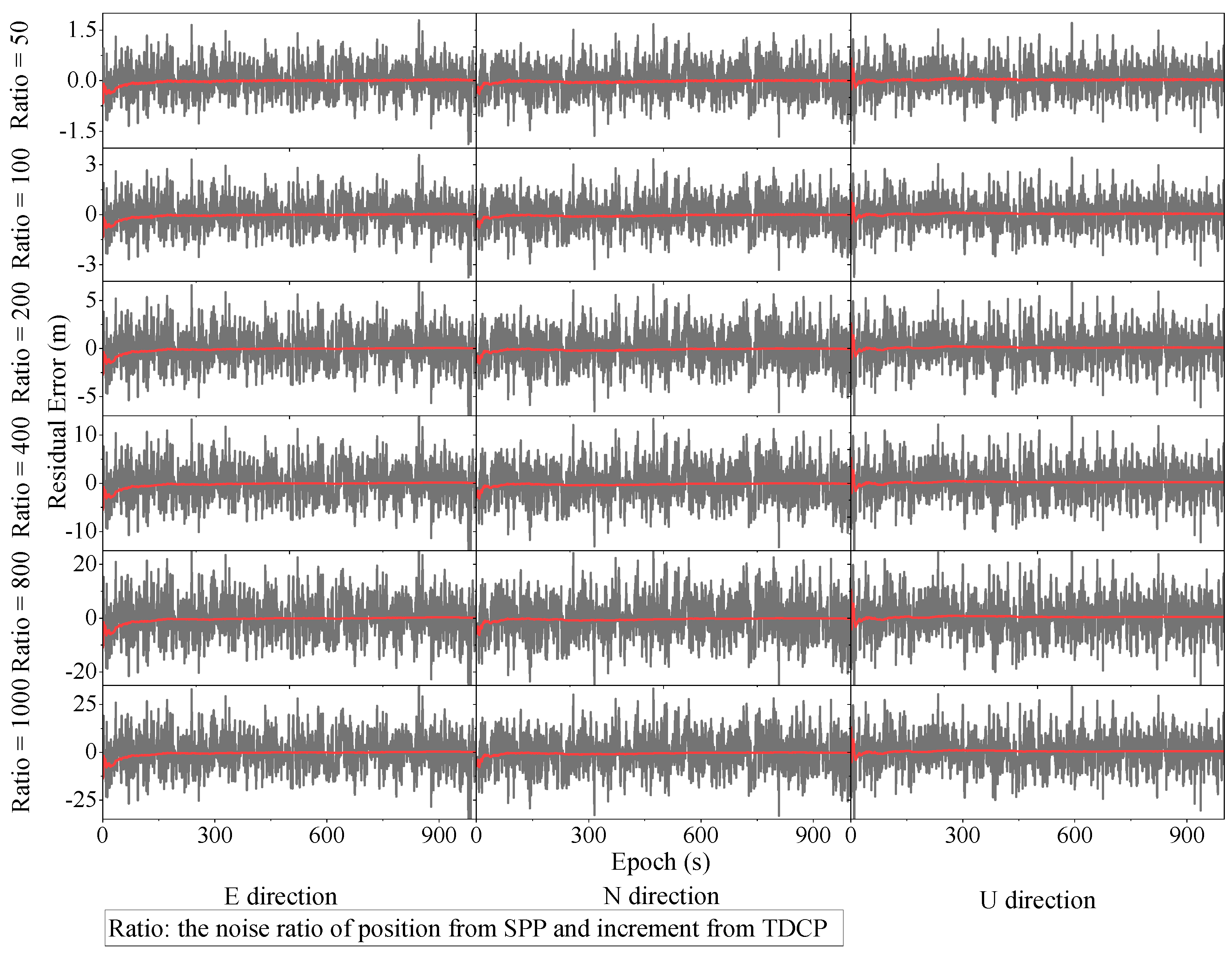
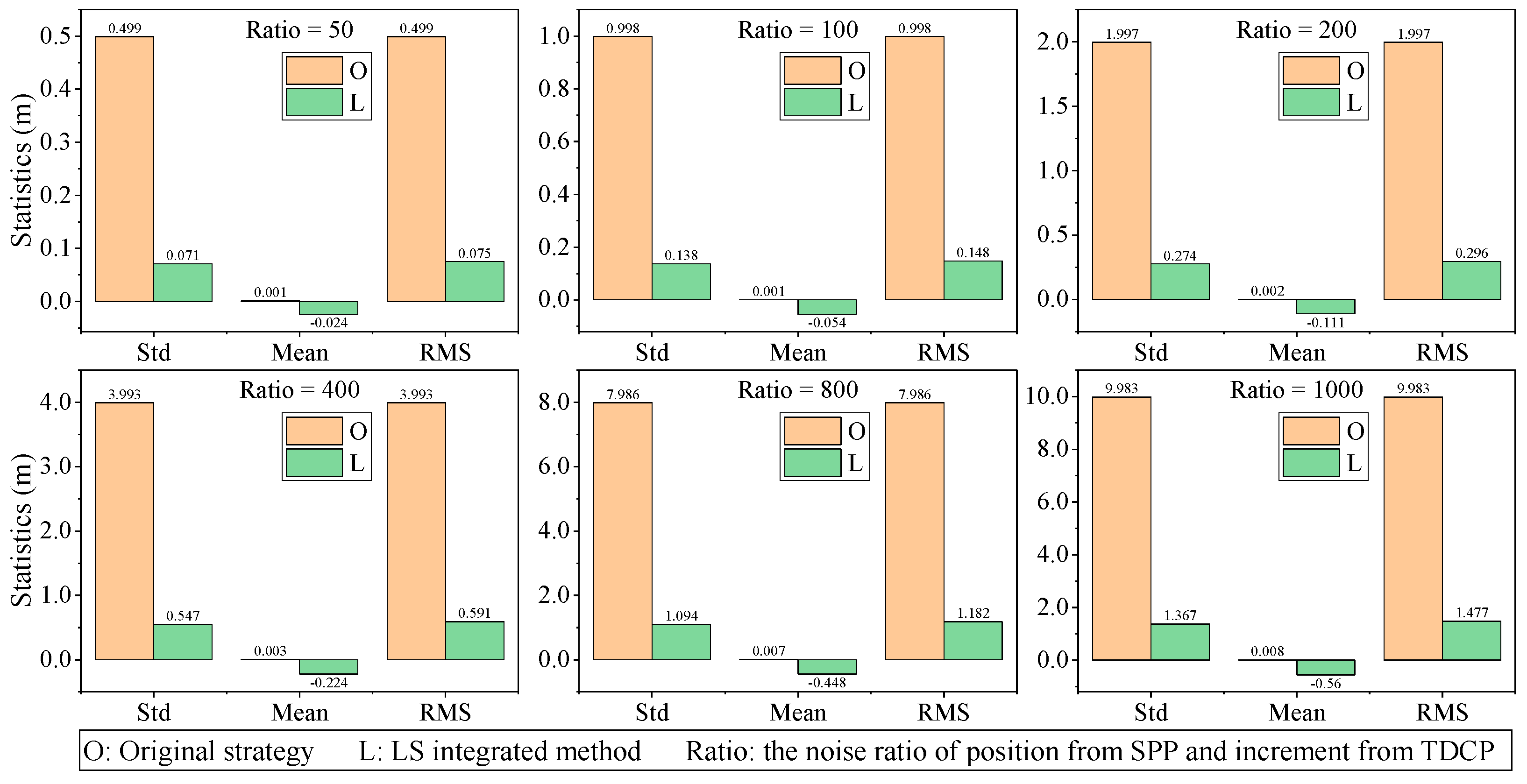
4.1.2. Experimental Analysis

The simulation experiment added different levels of Gaussian white noise to both the position and its increment (position time difference) data to simulate the GNSS solutions from SPP and TDCP, where the noise added to the increment had set with a standard deviation (Std) of 0.01 m to ensure controlled variability and various noise levels (50 to 1000 times the increment noise) was set for position solution. The simulation experiment simulated the GNSS solutions from SPP and TDCP by adding Gaussian white noise with different levels (50 to 1000 times the increment noise) to the high-accuracy position and its increment (position time difference) data, which had a standard deviation (Std) of 0.01 m for the increment noise. The experiment then integrated the simulated position and its increment data using the LS position domain filtering algorithm with different numbers of epochs to examine its performance with different temporal settings. Then, the experiment converted this optimized trajectory to the local coordinate system and analyzed the performance of the position domain from the LS method with multi-epochs by evaluating the residual positioning errors in the E, N, and U directions for different noise levels. This study used the QELS to represent various MELS for a focused and efficient comparison because a previous study [24] revealed subtle differences among various MELS.
To validate the effectiveness of the LS integrated method within the position domain, the results are presented in Figure 3, where the residual errors of both the original positioning strategy and the LS integrated method are compared. It is observed that the LS integrated method exhibits a remarkable improvement in performance characterized by a rapid convergence rate. The position accuracy achieved through the integration process surpasses the original positioning strategy. This enhanced accuracy is observed even during scenarios of unconverted states or when multiple epochs are required for convergence. The LS integrated method consistently provides a relatively stable solution, demonstrating its robustness in addressing positioning challenges.
To substantiate the efficiency of the LS integrated method, a thorough investigation was conducted based on statistical analysis by computing the Std, mean value, and Root Mean Square (RMS) of both the original positioning strategy and the LS integrated method. The accuracy statistics in the E direction of this analysis are summarized in Figure 4, and the N and U are not revealed for similar statistical results. These findings reveal the efficacy of the LS integrated method in significantly enhancing positioning accuracy and stability compared to traditional positioning strategies. The comparative analysis presented in both Figure 3 and Figure 4 reveal striking disparities between the Std and RMS values of the LS integrated method and those of the original positioning strategy. These disparities highlight the substantial performance improvement achieved through the application of the LS integrated method. It is worth noting that while the Std and RMS values significantly decrease with the LS integrated method, the mean value exhibits a noticeable increase. This increase is primarily attributed to the convergence process, which results in reduced residuals and an asymmetric distribution of positioning errors. The combined insights from Figure 3 and Figure 4 collectively indicate that the position domain integration method can effectively reduce the noise level in position results by approximately 10% when compared to the original positioning strategy. This reduction is theoretically achieved after several epochs, signifying the method’s capability to rapidly achieve convergence over a short time. Furthermore, the study reveals that the LS integrated method delivers more pronounced improvements in positioning accuracy, particularly for receivers with lower precision. The vertical comparison results highlight that the positioning accuracy of the LS integrated method diminishes as the position noise introduced by the strategy increases. This reveals the sensitivity of positioning accuracy, where different LS methods may yield superior performance for receivers with varying levels of precision. Furthermore, it is observed that the accuracy of horizontal (E and N direction) components is of a similar level to the vertical (U direction) component, which can be attributed to the fact that the simulated experiment introduces an equivalent level of noise to the X, Y, and Z coordinates, resulting in the transformation of the error ellipsoid into a more symmetric spherical shape. In summary, the comprehensive analysis presented in both Figure 3 and Figure 4 underscores the effectiveness of the LS integrated method in significantly reducing positioning errors and enhancing accuracy, particularly in scenarios involving receivers with varying precision levels.
This study presents the theoretical analysis and simulation results of the LS filtering method for GNSS positioning. Figure 5 shows the theoretical precision curve, which represents the filter accuracy as a function of the noise level of the position obtained by the SPP technology. The curve indicates that the filter accuracy increases as the noise level decreases, which is consistent with the intuition that the lower the noise, the higher the precision. Moreover, the LS filtering algorithm achieves a better solution by increasing the number of filtering epochs, which is the number of times that the filter updates the position estimate based on the measurements. The filter result depicted in Figure 5 agrees with the experimental results obtained from the simulation datasets, which demonstrate that the filtering accuracy converges to a stable value with a decreasing convergence speed as the filtering time increases. This implies that the LS filtering method is a convergent filter, which means that it can reach a consistent and optimal solution after a finite number of iterations. In addition, Figure 5 reveals that the LS filtering method provides high convergence accuracy for the GNSS receivers with better performance and a corresponding position result for the receivers with lower performance. However, the receivers with lower performance can also attain the same performance as the receivers with higher performance by extending the number of filtering epochs to a certain degree. This section only validates the effectiveness of the LS filtering method by using a simulated dataset and theoretical analysis while ignoring some error sources that may exist in practical engineering applications, such as multipath, ionospheric delay, and atmospheric effects. These error factors may affect the filter accuracy and the convergence rate of the LS filtering method. Therefore, in the next section, we will test the LS filtering algorithm with the real measured dataset collected from different scenarios and compare it with the existing methods.

4.2. Real Measured GNSS Dataset Study under an Open Environment

In this section, the real measured GNSS dataset under a leaky environment was used to test and verify the observation and position domain filtering method by LS integrating methods based on different epochs.

4.2.1. GNSS Dataset Processing Model

Practical engineering applications involve various error sources that affect filter accuracy and positioning reliability. Environmental conditions, such as multipath, ionospheric effects, and signal attenuation, can introduce non-Gaussian noise and biases into GNSS measurements. GNSS receiver performance can also vary based on hardware quality, antenna characteristics, chipset, firmware, signal processing, and error correction. These factors require receiver-specific filtering methods and real-time or near-real-time processing. Therefore, position domain filtering methods, especially LS-based ones, need rigorous testing and validation using real GNSS data under diverse scenarios. To assess the robustness and applicability of the LS methods in real-world scenarios, the GNSS data of the controlled experiment, same with simulation data, were analyzed, focusing on a diverse array of GNSS combinations: G (GPS), GC (GPS, BDS), GR (GPS, GLONASS), GE (GPS, Galileo), GRE (GPS, GLONASS, Galileo), GRC (GPS, GLONASS, BDS), GCE (GPS, BDS, Galileo), and GREC (GPS, GLONASS, Galileo, BDS). This approach ensures a thorough examination of the LS methods’ performance across various GNSS systems, thereby reflecting real-world GNSS operation scenarios. The settings for the double difference (DD) model and SPP model for the GNSS dataset processing are presented in Table 1. The experimental testing under a leaky environment is consistent with the data used in simulation scenarios, which has been well documented in the previous statement.

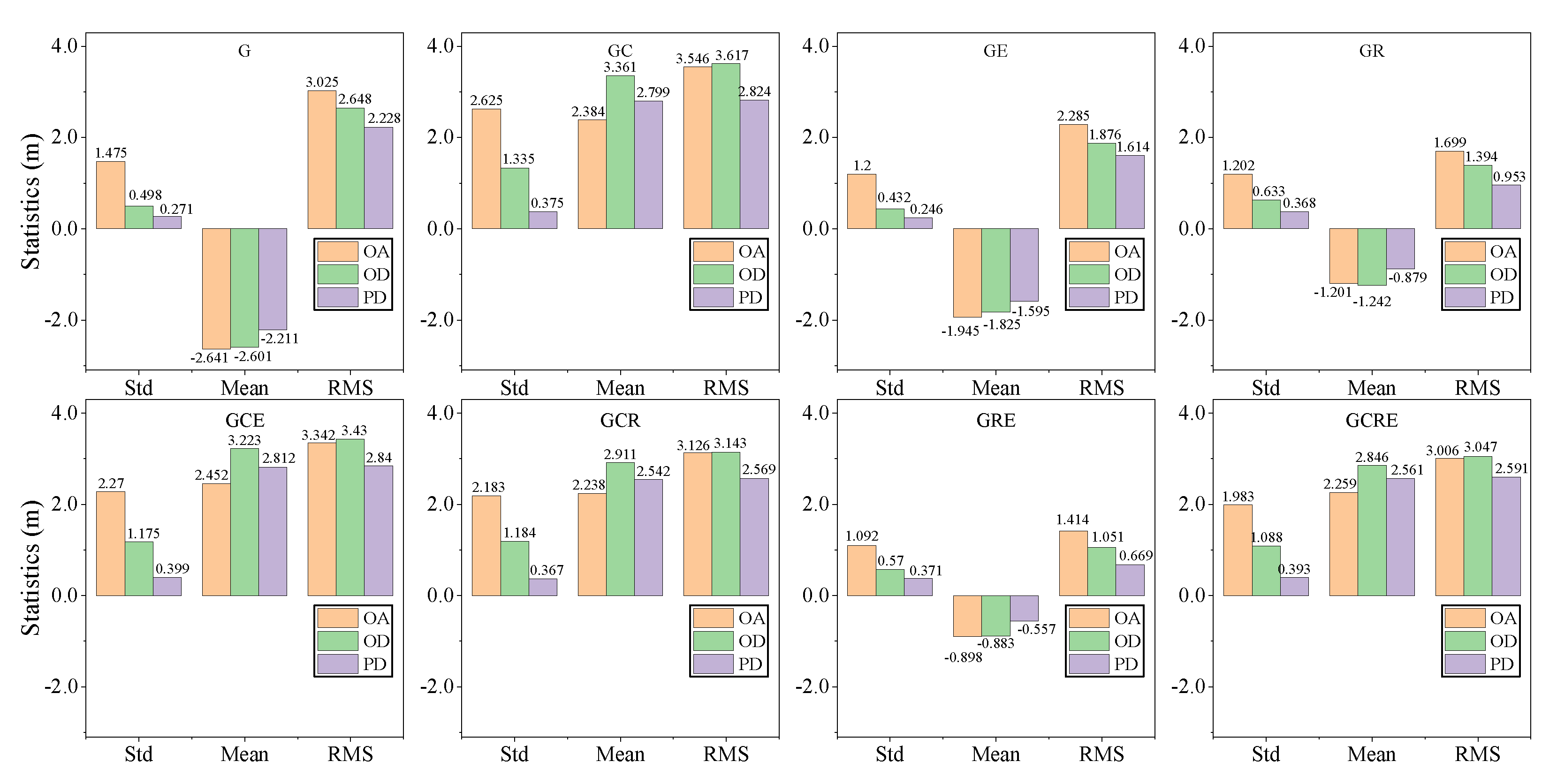
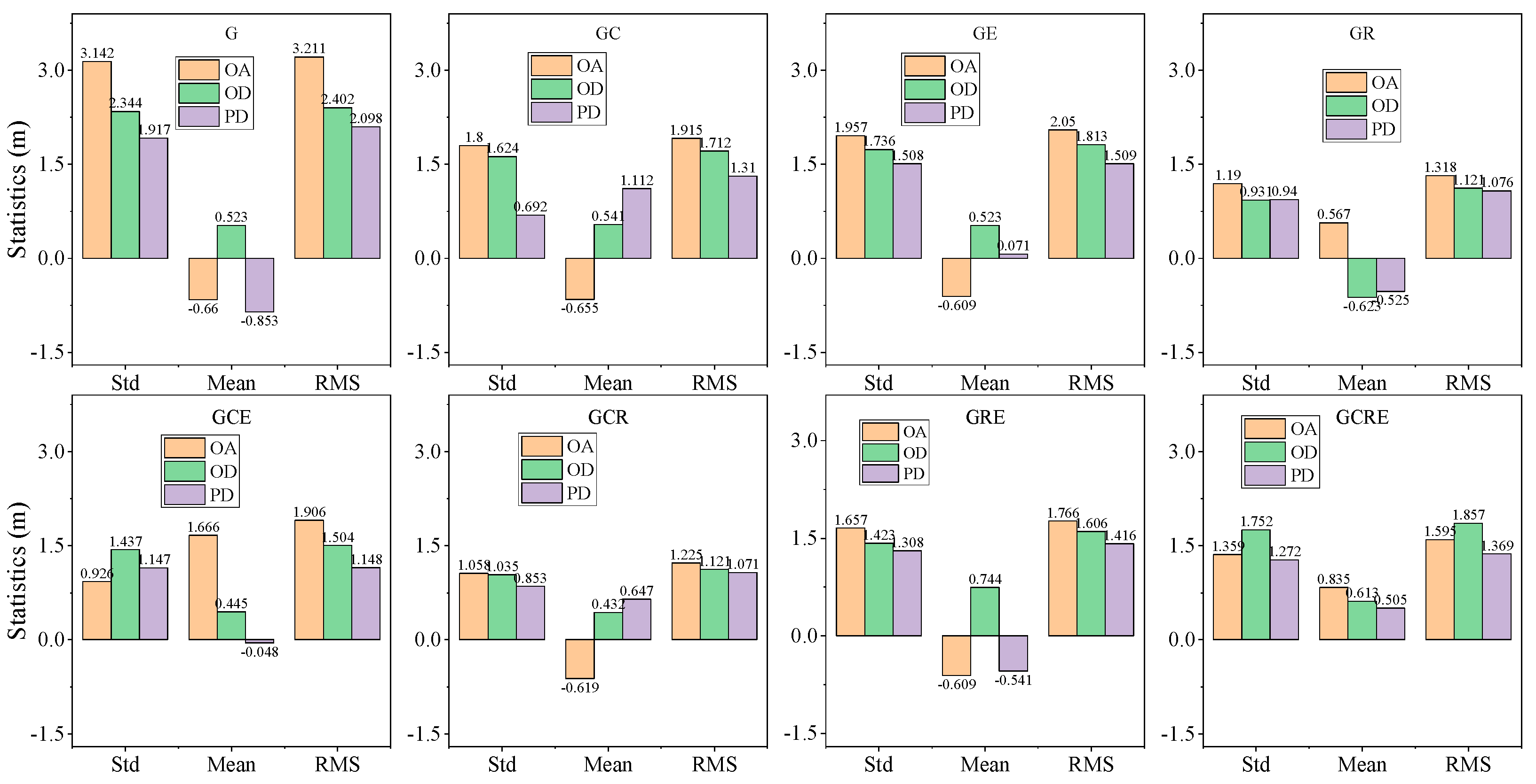
4.2.2. Performance Comparison of Observation and Position Domain Filtering Method

The PPPH, developed by Bahadur [56], was modified and then developed to implement all of the LS integrating method in this paper. Within the observation domain, we set the noise level for carrier phase observations at 3 mm, ensuring the high precision required for the investigation. For pseudorange observations, we determined the noise levels based on a statistical analysis that considered the time difference between pseudorange and carrier phase observations. This tailored approach ensured that the noise levels were accurately calibrated to the specific parameters of the experimental setup. Turning to the position domain, as indicated in Figure 6, Figure 7 and Figure 8, we defined the noise level for position increments at 0.01 m, maintaining a high degree of precision essential for analysis. As compared to the original algorithm and position domain, we set the position noise to be 50 to 1000 times the increment noise, allowing for an evaluation of the filtering methods. In this study, we used the double epoch LS (DELS) method instead of the LS method for the outcome from Li et al. [24] which demonstrated minimal differences between DELS, triple epoch LS (TELS), and quadra epoch LS (QELS) methods. It should be noted that the reference truth from the GNSS fusion double difference model was set as the coordinate origin to establish local coordinates, and then the coordinates of the positioning results obtained from the original algorithm, observation and position domain filtering method were projected to compute the E, N, and U direction errors.
The positioning solutions obtained by the original SPP technology, observation domain, and position domain filtering methods for various GNSS combinations are presented in Figure 6, Figure 7 and Figure 8, along with their Std, mean, and RMS values. These results show that different GNSS combinations, with their respective accuracy solutions, can achieve high-precision and reliable positioning performance. The average Std values for the original algorithm in the E, N, and U directions were 0.535 m, 0.653 m, and 1.754 m, respectively. The corresponding mean values were 0.317 m, 0.712 m, and 0.331 m, while the RMS values were 0.631 m, 1.076 m, and 2.680 m. The statistical information suggests that the horizontal directions (E and N) generally perform better than the vertical (U) direction, which can be explained by the geometric distribution of GNSS satellites. Among the horizontal directions, the E direction often performs better than the N direction due to the geographic location of the GNSS receiver (latitude, longitude) and the related satellite constellation geometry [57]. Overall, using a multi-GNSS combination tends to improve accuracy and robustness compared to a single-GNSS approach, with accuracy mainly influenced by the number of positioning satellites available. The GNSS precision is enhanced significantly when integrating GLONASS and Galileo, indicating the crucial role of these two systems in improving positioning accuracy. For the Std values, the smallest values in the E, N, and U directions were obtained for the GRE, GE, and GRE system combinations, with values of 0.293 m, 0.437 m, and 1.092 m, respectively. On the other hand, the largest Std values in all three directions were related to the GC combination, with values of 0.843 m, 0.954 m, and 2.625 m for E, N, and U, respectively. For the mean values, the smallest values in the E, N, and U directions were observed for the GCRE, GCE, and GRE combinations, with values of 0.189 m, 0.006 m, and 0.898 m, respectively. On the contrary, the largest mean values in all three directions were associated with the G system, with values of 0.696 m, 1.572 m, and 2.641 m for E, N, and U, respectively. For the RMS values, the smallest values in the E, N, and U directions were again obtained for the GRE, GCRE, and GRE combinations, with values of 0.358 m, 0.675 m, and 1.414 m, respectively. In contrast, the largest RMS values in the E, N, and U directions were G, G, and GC combinations, with values of 0.929 m, 1.738 m, and 3.546 m, respectively. It is important to note that the inclusion of BDS can reduce positioning accuracy due to the multipath effect of GEO (Geosynchronous Earth Orbit) satellites, which can be difficult to remove through parameter estimation. However, the accuracy could be improved by modeling the multipath error of GEO satellites more precisely. Moreover, the contribution of Galileo is expected to be even more significant in positioning accuracy as the satellite constellation becomes fully operational. Nevertheless, this study mainly focuses on comparing the accuracy of the DELS method based on position and observations, and the performance of the original SPP algorithm is beyond the scope of this research.
Focusing on the observation domain integrated DELS approach, the observation domain integrated DELS approach shows average Std values of 0.245 m, 0.330 m, and 0.864 m in the E, N, and U directions, respectively, as well as corresponding mean values of 0.243 m, 0.614 m, and 0.724 m, and RMS values of 0.353 m, 0.886 m, and 2.526 m. On the other hand, the position domain integrated DELS method produces average Std values of 0.159 m, 0.499 m, and 0.349 m in the E, N, and U directions, respectively, along with mean values of 0.080 m, −0.123 m, and 0.684 m, and RMS values of 0.202 m, 0.843 m, and 2.036 m. These three statistical parameters demonstrate the effectiveness of both integration methods in enhancing the overall 3D accuracy in GNSS applications. Moreover, it is noted that while the 3D accuracy is generally improved, some specific directional accuracies may have slight decreases under certain conditions. For a more comprehensive assessment of the performance of the position domain integrating method using DELS, it is contrasted with the original algorithm and the observation domain integrating method based on DELS.
Focusing on the Std, mean, and RMS enhanced by position domain compared with the original algorithm, observation domain based on DELS, the position domain method improves the positioning precision consistently in all statistical parameters compared with the original algorithm and the observation domain based on DELS. The position domain method achieves remarkable advancements in positioning accuracy relative to the original algorithm despite some occasional reductions in accuracy. Compared with the original algorithm, the observation domain showed average percentage improvements in the Std values for the E, N, and U directions of 54.2%, 49.4%, and 50.7%, respectively, while the mean and RMS values decreased by about 23.1%, 13.8%, −17.9% and 44.0%, 17.7%, 5.8%, respectively. Compared with the original algorithm, the positioning domain achieved average percentage improvements in the Std values for the E, N, and U directions of 70.3%, 23.6%, and 80.1%, respectively, and in the mean and RMS values of 70.6%, 10.4%, 0.4%, and 68.0%, 21.6%, 24.0%, and also showed further improvements over the observation domain in the Std values of 16.1%, −25.9%, and 29.4%, respectively, and in the mean and RMS values of 47.5%, −3.4%, 18.3% and 24.0%, 4.0%, 18.3%, respectively. These findings support the enhanced positioning accuracy of the position domain integrating method compared to both the original algorithm and the observation domain integrating method, with RMS values emerging as the most effective indicator of positioning accuracy due to their comprehensive reflection of changes in both mean and standard deviation.

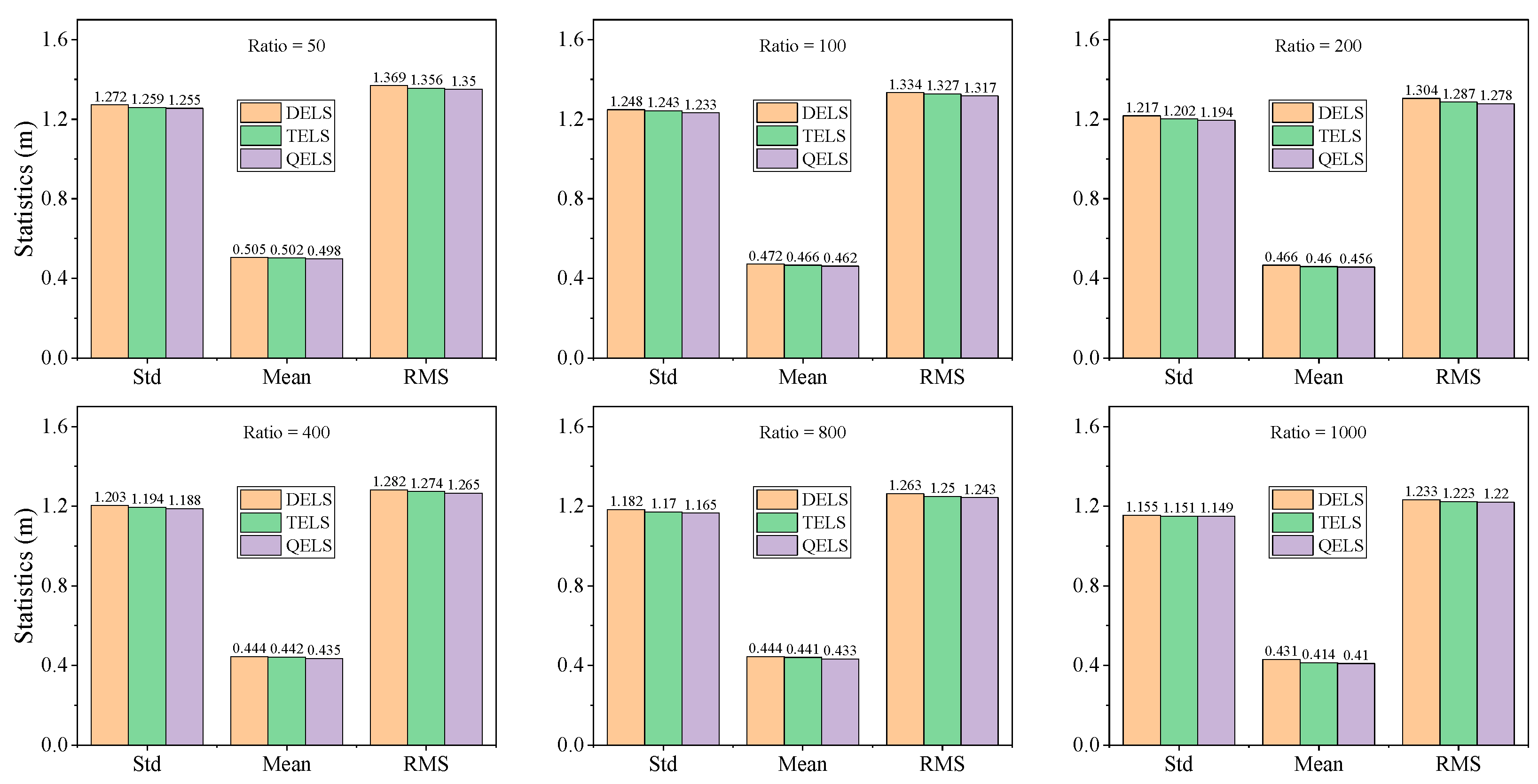
4.2.3. Performance Comparison of MELS Based on the Position Domain Filtering Method

To conduct a thorough evaluation of position domain filtering methods employing the LS approach with different epoch configurations, an analysis of the positioning performance was undertaken, focusing only on one satellite system, GPS-only positioning. This analysis focused on assessing the Std, mean, and RMS values associated with three distinct epoch configurations: DELS, TELS, and QELS. This evaluation included various epochs with varying weight ratios between the position and the increment components. Figure 9, Figure 10 and Figure 11 present the DELS, TELS, and QELS performance comparison of the LS-based position domain filtering methods with various epoch strategies for GPS-only positioning.
The position domain filtering methods based on the LS integration approach are comprehensively analyzed in Figure 9, Figure 10 and Figure 11, with a focus on the effects of varying the number of epochs and the weight ratio between the original algorithm’s position estimate and its increment on the statistical characteristics, including Std, mean, and RMS values. The figures offer valuable insights into the optimization of these LS-based methods for enhancing positioning accuracy within the framework of a single-system GNSS. The analysis of the results indicates that the DELS method with the lowest weight ratio achieves the minimum Std values in the E and N directions, with values of 0.165 m and 0.451 m, respectively. On the contrary, for the U direction, the QELS method with a weight ratio obtains the minimum Std value of 0.257 m. On the other hand, the maximum Std values in the E and N directions are associated with the highest weight ratio in the QELS method, resulting in values of 0.173 m and 0.511 m, respectively, while for the U direction, the DELS method with the minimum weight ratio shows the maximum Std value, measured at 0.271 m. It is also observed that the TELS integrated method outperforms DELS, with QELS showing a slight improvement over TELS in all directions, usually on the order of several millimeters. This suggests that the precision in position domain filtering methods increases proportionally with the addition of more epochs. Interestingly, the strategy for enhancing horizontal precision differs from that applied to elevation when expanding epochs for LS methods. Moreover, the figure reveals a significant inverse relationship between Std and mean values. The adjustment of the weight ratio between the original algorithm’s position and its increment strongly influences the positioning accuracy. In this context, all statistical parameters (Std, mean, and RMS) exhibit a consistent reduction as the weight ratio is increased. This implies that the accuracy of the original strategy decreases as the positioning accuracy in all directions improves. The distribution of weights and the stochastic model become more suitable as the weight ratio decreases. However, it is important to emphasize that a higher weight ratio may reduce the impact on accuracy, indirectly indicating the high accuracy of the TDCP calculation increment. Yet, it is also important to note that the accuracy gains may level off or even decrease when the weight ratio is excessively increased. Therefore, determining a suitable weight ratio for each epoch, informed by the standard positioning strategy and TDCP, has the potential to produce optimal results in the position domain filtering method. This nuanced approach to weight distribution within the stochastic model is essential for improving and enhancing the accuracy of GNSS.

4.3. Real Measured GNSS Dataset Study under Forest Scene

This section tested the observation and position domian method based on the real measured GNSS dataset under a forest environment, which was collected at an artificially planted forest at NWAFU, mainly planted with beech trees.

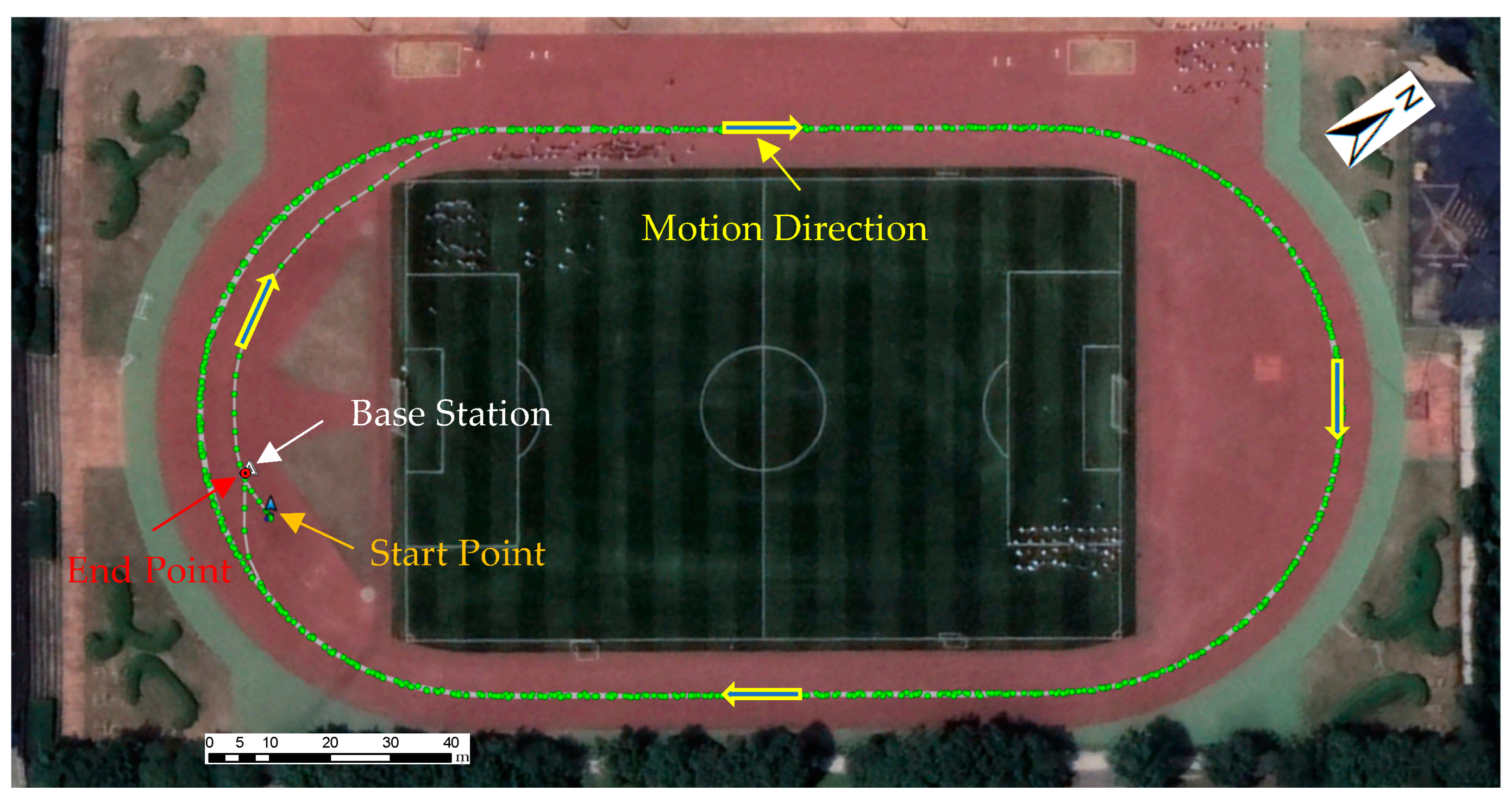
4.3.1. Dataset Description

This section analyzed the performance comparison between observation and position domain filtering methods using the MELS integrating technique in a shadow environment. The analysis used the trajectory data of a vehicle with a GNSS receiver that drove through an artificial plantation at Northwest A&F University, located at Latitude 34°15′45″ and Longitude 108°03′34″. The experiment was conducted on 19 March 2023 (DOY 078), where a BDStar (Beijing BDStar Navigation Co., Ltd., Beijing, China) M68 GNSS receiver recorded continuously over approximately 2100 s, with a consistent sampling frequency of 1 Hz. This real-world dataset and consistent experimental conditions aimed to reveal the relative effectiveness and performance of observation versus position domain filtering methods when applied to the MELS integrating technique in a forest scene. To get the reference value for the SPP solution, this study set up a GNSS reference station on the roof of the College of Forestry, NWAFU. The reference station was observed for 4 h, covering the whole observation period of the rover, and Figure 12 shows the trajectory of the rover in the forest scene and the base station.
The receiver started from the origin and moved to the southeast corner of the beech square, then entered the forest and made 23 round trips before reaching the northwest corner of the forest group. After that, it circled the forest and returned to a point near the origin. The beech forest group is an artificial plantation with neatly arranged trees, pedestrian paths under the trees, and benches and tables along the paths for entertainment. The motion trajectory in the figure shows many sharp points, which are caused by the following reasons: (1) severe forest occlusion introduced gross errors in the GNSS observations, and the data processing algorithm failed to fully eliminate these errors, resulting in inaccurate data; (2) the data collector held the center pole, which was constantly shaking during the data collection, causing sharp points in both elevation and horizontal directions; (3) the data collector had to avoid obstacles such as benches during the data collection, resulting in non-linear motion trajectories. Figure 13 shows the variations in positioning along E, N, and U directions, with the barycentric coordinates as the origin of the coordinate system. The data collection area is close to the poles, so the north direction has a jagged pattern, while the E direction has a step-down pattern. As the receiver moves around the square, the position changes in the north or south direction are minimal, and the elevation changes are due to the same reasons as the sharp points above.

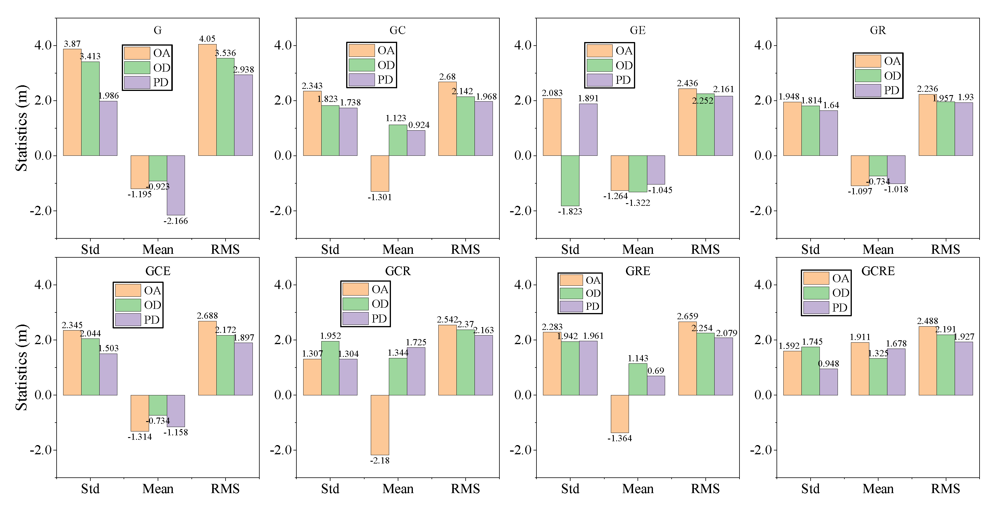
4.3.2. Performance Comparison of Observation and Position Domain Filtering Method

The data processing settings in this part are similar to those in the open environment, except that we set the cutoff elevation angle to 30 degrees. With the help of a large number of satellites from various systems, especially the visible number of BDS satellites in China, we can still obtain a large number of available satellites in this scenario. This study uses the positioning results from the double-difference model as the reference truth. It evaluates the positioning accuracy of the original algorithm, the observation-domain filtering method, and the position-domain filtering method under different GNSS combinations. The results are shown in Figure 14, Figure 15 and Figure 16.
This section uses different combinations of GNSS and adopts the original SPP technology, observation domain, and position domain filtering methods to obtain the positioning solutions, and shows their STD, mean, and RMS in Figure 14, Figure 15 and Figure 16, indicating the positioning situation is similar to the conclusion drawn from the open scenario. These results show that different GNSS combinations result in different accuracy solutions, which can achieve high precision and reliable positioning performance, and the positioning accuracy in the upward direction is lower than that in the east and north directions, which is similar to the forest scenario. This is a common feature of GNSS positioning. The figure displays the positioning accuracy values of each combination of the GNSS system and filtering method in the east, north, and upward directions, as well as the percentage of positioning accuracy improvement of each filtering method relative to the original SPP technology and observation domain filtering method. The original algorithm has a positioning accuracy of 1.863 m, 1.873 m, and 2.722 m in the E, N, and U directions, respectively. The observation domain filtering method increases the accuracy by 12.2%, 14.1%, and 15.4%, resulting in 1.661 m, 1.642 m, and 2.359 m, respectively. The position domain filtering method further increases the accuracy by 27.0%, 19.4%, and 10.6%, resulting in 1.308 m, 1.375 m, and 2.133 m, respectively. This method achieves an overall improvement of 42.4%, 36.2%, and 27.6% compared to the original algorithm. The above results show that the filtering methods can significantly improve the positioning performance, and the positioning performance in the forest scenario is similar to that in the open scenario, which means that the filtering methods can effectively reduce the influence of the forest environment, such as signal attenuation, multipath, and interference. The experimental results of measured data under the forest show that the position domain filtering method is also adaptable to the occluded environment.

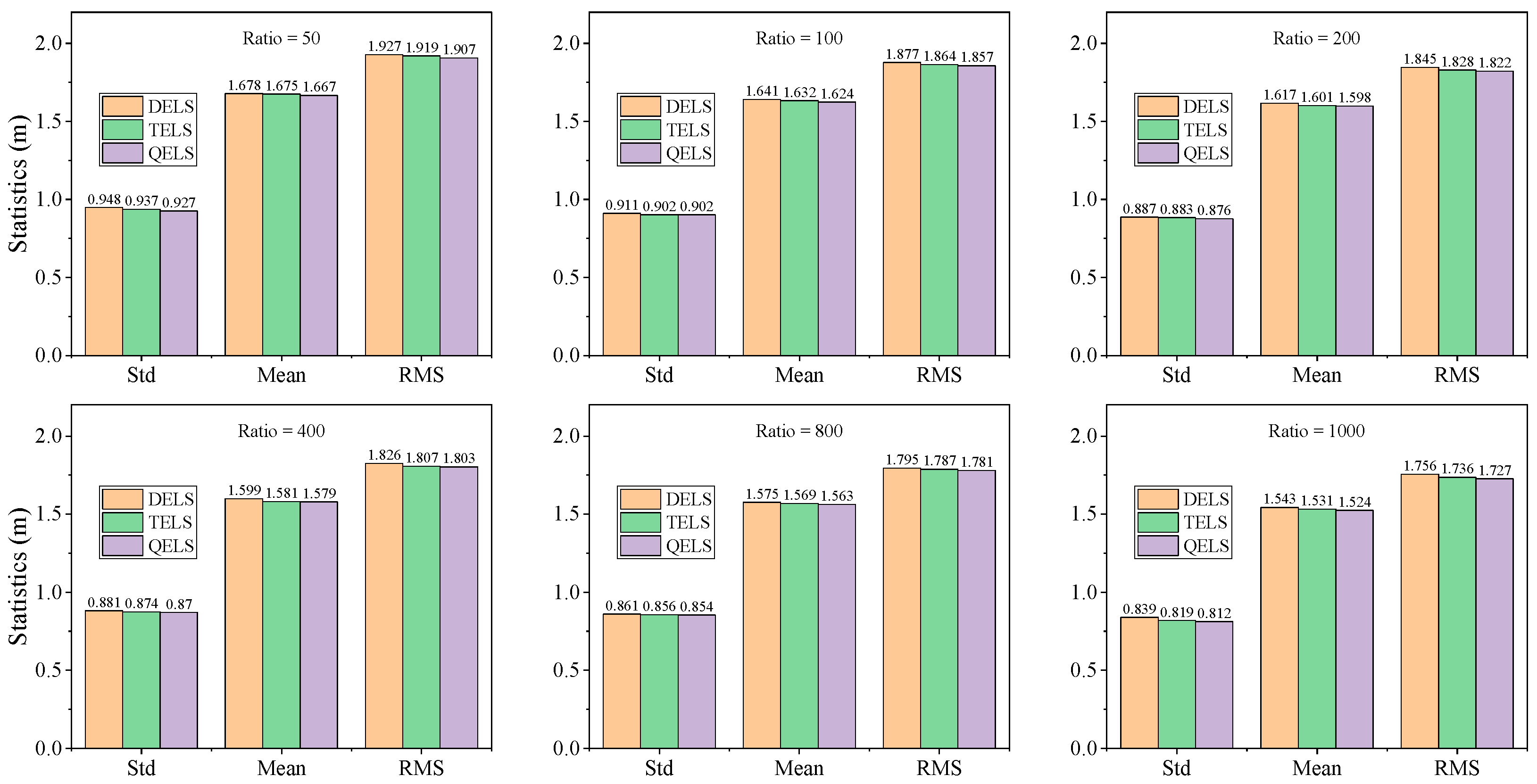
4.3.3. Performance Comparison of MELS Based on the Position Domain Filtering Method

The performance of position domain filtering methods using the LS approach was evaluated in the forest scenario with different epoch configurations and GCRE combinations. The Std, mean, and RMS values for three epoch configurations (DELS, TELS, and QELS) were assessed in this analysis. The evaluation also considered different epochs with different weight ratios between the position and the increment components. The performance comparison of the LS-based position domain filtering methods for GPS-only positioning with different epoch strategies is shown in Figure 17, Figure 18 and Figure 19.
Figure 17, Figure 18 and Figure 19 comprehensively analyze the position domain filtering method based on the LS integration method using under-canopy semi-shaded data, focusing on the impact of changing the number of epochs and the weight ratio between the position estimation and its increment of the original algorithm on the statistical characteristics, including Std, mean and RMS values, providing valuable insights for the optimization of these LS-based methods. The result analysis shows that the adjustment of the weight ratio between the position and its increment of the original algorithm strongly affects the positioning accuracy. As the positioning accuracy in all directions improves, the accuracy of the original strategy decreases, and as the weight ratio decreases, the weight distribution and random model become more suitable, which is significantly different from the open environment. It may be caused by the fact that the probability of gross errors in the observations increases significantly due to the under-canopy shading environment. For TDCP technology, only a small amount of satellite data is required, and no gross errors are guaranteed to achieve the position increment solution; even under the canopy, we can still observe a large number of satellites, and it is relatively easy to filter out the carrier data without gross errors in this part of the data. For pseudorange observations, a large number of observations are required to improve the positioning accuracy and reliability, and the difficulty of processing all observation gross errors is relatively large. It is also observed that the TELS integrated method is superior to the DELS, and the QELS is slightly improved over the TELS in all directions. Similar differences are presented in the standard deviation, mean, and RMS, and their order of magnitude is usually in the sub-centimeter. This indicates that the accuracy of the position domain filtering method increases proportionally with the increase of more epochs. However, it is important to emphasize that a higher weight ratio can reduce the impact on accuracy, indirectly indicating the high accuracy of TDCP calculation increment, and it is also important to note that when the weight ratio is excessively increased, the accuracy gain may tend to be stable or even decrease. Therefore, according to the standard positioning strategy and TDCP, it is possible to produce the best results in the position domain filtering method by determining the appropriate weight ratio for each epoch. This subtle treatment of the weight distribution in the random model is crucial for improving and enhancing the accuracy of GNSS, which is similar to the results tested in the open environment.

5. Conclusion and Future Work

In pursuit of heightened positioning accuracy and the broader utilization of GNSS, this study has undertaken a comprehensive validation of the efficacy of a position domain filtering method based on the standard positioning strategy and TDCP technology, employing the LS approach. The performance of this method has been rigorously compared with that of the observation domain filtering method, which formulates a meticulous mathematical and stochastic model rooted in error propagation principles during the acquisition of LS solutions. To ascertain the effectiveness of the position domain filtering method, a rigorous assessment was conducted, encompassing both simulated and real measured datasets. The simulated data revealed that the position domain strategy consistently yields smaller RMS values when juxtaposed with the original strategy. Furthermore, experimental results from kinematic GNSS datasets recorded in open environment and forest scenes show that the observation domain integrating method outperforms the original strategy, and the position domain integrating method outperforms the observation domain integrating method, manifesting as a significant performance improvement. The experimental results in an open environment show that the original algorithm has positioning accuracies of 0.631 m, 1.076 m, and 2.680 m in the E, N, and U directions, respectively. The observation domain filtering method improves the accuracies by 44.0%, 17.7%, and 5.8%, compared to the original algorithm, resulting in 0.353 m, 0.886 m, and 2.526 m, respectively. The position domain filtering method further improves the accuracies by 68.0%, 21.6%, and 24.0%, compared to the original algorithm, resulting in 0.202 m, 0.843 m, and 2.036 m, respectively, and achieving an overall improvement of 68.0%, 21.6%, and 24.0%, compared to the original algorithm. Also, the experimental results under the forest show that the positioning accuracies based on the original algorithm are 1.863 m, 1.873 m, and 2.722 m in the E, N, and U directions, respectively. The positioning accuracies based on the observation domain filtering method are 1.661 m, 1.642 m, and 2.359 m in the E, N, and U directions, respectively, which are 12.2%, 14.1%, and 15.4% higher than the original algorithm accuracies, respectively. The accuracies based on the position domain filtering method are 1.308 m, 1.375 m, and 2.133 m in the E, N, and U directions, respectively, which are 42.4%, 36.2%, and 27.6% higher than the original algorithm accuracy, respectively, and 27.0%, 19.4% and 10.6% higher than the position domain positioning accuracies. These compelling results unequivocally affirm that the observation domain filtering method constitutes a significant advancement, substantially bolstering positioning accuracy and extending the frontiers of GNSS applications.
Nevertheless, it is important to acknowledge that the position domain filtering methods used in this study have two inherent limitations. First, the model does not currently account for the correlation between the position increments derived from the TDCP technique, even though both pieces of information are intrinsically related to the carrier phase observations of the intermediate epoch. Second, the model assigns the same variance information to the three directions of the positioning results generated by the standard positioning strategy, ignoring their interrelationship. As part of the ongoing research work, we are committed to improving the existing model to fully address these overlooked errors. The goal is to develop a more robust and complex stochastic model that can not only correct these limitations but also enhance the overall accuracy and reliability of the positioning accuracy, as well as meet certain production applications. This ongoing work represents the dedication to advancing the state-of-the-art global navigation satellite system positioning technology and applying it to smart forestry while ensuring its continuous effectiveness in practical engineering production applications.

Author Contributions

Conceptualization, F.L., J.Y. and J.G.; methodology, F.L. and X.M.; software, F.L. and J.Y.; validation, Q.L., J.Y. and X.K.; writing—original draft preparation, F.L. and J.Y.; writing—review and editing, F.L., P.P. and X.M.; revision, F.L., P.P. and X.M.; supervision, J.G., P.P. and X.M.; funding acquisition, F.L., Q.L., L.N. and X.K. All authors have read and agreed to the published version of the manuscript.

Funding

This work was partially supported by the National Key Research and Development Program of China (2023YFC3209101), Natural Science Basic Research Program of Shaanxi (2023-JC-QN-0250), Chinese Universities Scientific Fund (2452022031, 2452022139), Scientific Research Program funded by Shaanxi Provincial Education Department (23JE014), Shaanxi Provincial Philosophy and Social Science Research Project (2023HZ1552), and National Science Foundation of China (41974026).

Data Availability Statement

Data are contained within the article.

Acknowledgments

The authors wish to extend their sincere appreciation to the International GNSS Service organization for granting access to invaluable datasets, as well as to the GNSS receiver provided by China University of Mining and Technology, and also for the GNSS receiver and high-performance computing provided by Northwest A&F University. Additionally, the authors express their gratitude to the editors for their valuable and constructive comments, which have undoubtedly contributed to the refinement of this research work.

Conflicts of Interest

Authors, Qi Li, Xiaomei Kou, and Le Niu was employed by the company Power China Northwest Engineering Corporation Limited. The remaining authors declare that the research was conducted in the absence of any commercial or financial relationships that could be construed as a potential conflict of interest.

References

  1. Lee, T.; Bettinger, P.; Merry, K.; Cieszewski, C. The effects of nearby trees on the positional accuracy of gnss receivers in a forest environment. PLoS ONE 2023, 18, e0283090. [Google Scholar] [CrossRef]
  2. Feng, T.; Chen, S.; Feng, Z.; Shen, C.; Tian, Y. Effects of canopy and multi-epoch observations on single-point positioning errors of a gnss in coniferous and broadleaved forests. Remote Sens. 2021, 13, 2325. [Google Scholar] [CrossRef]
  3. Guo, J.; Hou, R.; Zhou, M.; Jin, X.; Li, C.; Liu, X.; Gao, H. Monitoring 2019 forest fires in southeastern australia with gnss technique. Remote Sens. 2021, 13, 386. [Google Scholar] [CrossRef]
  4. Garrido-Carretero, M.S.; Azorit, C.; de Lacy-Pérez de los Cobos, M.C.; Valderrama-Zafra, J.M.; Carrasco, R.; Gil-Cruz, A.J. Improving the precision and accuracy of wildlife monitoring with multi-constellation, multi-frequency gnss collars. J. Wildl. Manag. 2023, 87, e22378. [Google Scholar] [CrossRef]
  5. Kaartinen, H.; Hyyppä, J.; Vastaranta, M.; Kukko, A.; Jaakkola, A.; Yu, X.; Pyörälä, J.; Liang, X.; Liu, J.; Wang, Y.; et al. Accuracy of kinematic positioning using global satellite navigation systems under forest canopies. Forests 2015, 6, 3218–3236. [Google Scholar] [CrossRef]
  6. Konakoglu, B.; Yilmaz, V. Evaluating the performance of the static ppp-ar in a forest environment. J. Surv. Eng. 2024, 150, 05023006. [Google Scholar] [CrossRef]
  7. Wang, A.; Zhang, Y.; Chen, J.; Wang, H. Improving the (re-)convergence of multi-gnss real-time precise point positioning through regional between-satellite single-differenced ionospheric augmentation. GPS Solut. 2022, 26, 39. [Google Scholar] [CrossRef]
  8. Quddus, M.A.; Ochieng, W.Y.; Noland, R.B. Current map-matching algorithms for transport applications: State-of-the art and future research directions. Transp. Res. Part C Emerg. Technol. 2007, 15, 312–328. [Google Scholar] [CrossRef]
  9. Grewal, M.S.; Andrews, A.P.; Bartone, C.G. Global Navigation Satellite Systems, Inertial Navigation, and Integration; John Wiley & Sons: New York, NY, USA, 2020. [Google Scholar]
  10. Zumberge, J.; Heflin, M.; Jefferson, D.; Watkins, M.; Webb, F. Precise point positioning for the efficient and robust analysis of gps data from large networks. J. Geophys. Res. Solid Earth 1997, 102, 5005–5017. [Google Scholar] [CrossRef]
  11. Lee, H.K.; Rizos, C.; Jee, G.-I. Position domain filtering and range domain filtering for carrier-smoothed-code dgnss: An analytical comparison. IEE Proc. -Radar Sonar Navig. 2005, 152, 271–276. [Google Scholar] [CrossRef]
  12. Li, F.; Gao, J.; Zheng, N.; Pan, C.; Zhao, L. A novel dual-domain filtering method to improve gnss performance based on a dynamic model constructed by tdcp. IEEE Access 2020, 8, 79716–79723. [Google Scholar] [CrossRef]
  13. Hatch, R. The synergy of gps code and carrier measurements. In 3rd International Geodetic Symposium on Satellite Doppler Positioning; Physical Sciences Laboratory of New Mexico State University: Las Cruces, NM, USA, 1982; pp. 1213–1231. [Google Scholar]
  14. Hwang, P.Y.; McGraw, G.A.; Bader, J.R. Enhanced differential gps carrier-smoothed code processing using dual-frequency measurements. Navigation 1999, 46, 127–137. [Google Scholar] [CrossRef]
  15. Tang, W.; Cui, J.; Hui, M.; Deng, C. Performance analysis for bds phase-smoothed pseudorange differential positioning. J. Navig. 2016, 69, 1011–1023. [Google Scholar] [CrossRef]
  16. Kim, D.; Langley, R.B. The multipath divergence problem in gps carrier-smoothed code pseudorange. In Proceedings of the 47th Annual Conference of the Canadian Aeronautics and Space Institute, Ottawa, ON, Canada, 30 April–3 May 2000; pp. 161–163. [Google Scholar]
  17. Song, J.; Milner, C. Impact of multipath on code-carrier divergence monitor and threat space analysis for dual-frequency gbas. In Proceedings of the IEEE/ION PLANS 2020, Portland, OR, USA, 20–23 April 2020. [Google Scholar]
  18. Lee, H.K.; Rizos, C.; Jee, I. Design and analysis of dgps filters with consistent error covariance information. In Proceedings of the 6th International Symposium on Satellite Navigation Technology Including Mobile Positioning and Location Services, Melbourne, Australia, 22–25 July 2023; pp. 22–25. [Google Scholar]
  19. Mcgraw, G. Generalized divergence-free carrier smoothing with applications to dual frequency differential gps. Navigation 2009, 56, 115–122. [Google Scholar] [CrossRef]
  20. Closas, P.; Fernández-Prades, C.; Fernández-Rubio, J.A. Maximum likelihood estimation of position in gnss. IEEE Signal Process. Lett. 2007, 14, 359–362. [Google Scholar] [CrossRef]
  21. Closas, P.; Gusi-Amigo, A. Direct position estimation of gnss receivers: Analyzing main results, architectures, enhancements, and challenges. IEEE Signal Process. Mag. 2017, 34, 72–84. [Google Scholar] [CrossRef]
  22. Vincent, F.; Chaumette, E.; Charbonnieras, C.; Israel, J.; Aubault, M.; Barbiero, F. Asymptotically efficient gnss trilateration. Signal Process. 2017, 133, 270–277. [Google Scholar] [CrossRef]
  23. Qian, N.; Chang, G.; Gao, J. Gnss pseudorange and time-differenced carrier phase measurements least-squares fusion algorithm and steady performance theoretical analysis. Electron. Lett. 2019, 55, 1238–1241. [Google Scholar] [CrossRef]
  24. Li, F.; Gao, J.; Psimoulis, P.; Meng, X.; Ke, F. A novel dynamical filter based on multi-epochs least-squares to integrate the carrier phase and pseudorange observation for gnss measurement. Remote Sens. 2020, 12, 1762. [Google Scholar] [CrossRef]
  25. Parkinson, B.W.; Enge, P.; Axelrad, P.; Spilker, J.J., Jr. Global Positioning System: Theory and Applications, Volume ii; American Institute of Aeronautics and Astronautics: Reston, VA, USA, 1996. [Google Scholar]
  26. Singer, R.A. Estimating optimal tracking filter performance for manned maneuvering targets. IEEE Trans. Aerosp. Electron. Syst. 1970, AES-6, 473–483. [Google Scholar] [CrossRef]
  27. Lagakos, S.W.; Sommer, C.J.; Zelen, M. Semi-markov models for partially censored data. Biometrika 1978, 65, 311–317. [Google Scholar] [CrossRef]
  28. Zhou, H.; Kumar, K. A current statistical model and adaptive algorithm for estimating maneuvering targets. J. Guid. Control Dyn. 1984, 7, 596–602. [Google Scholar] [CrossRef]
  29. Moose, R. An adaptive state estimation solution to the maneuvering target problem. IEEE Trans. Autom. Control 1975, 20, 359–362. [Google Scholar] [CrossRef]
  30. Helferty, J.P. Improved tracking of maneuvering targets: The use of turn-rate distributions for acceleration modeling. IEEE Trans. Aerosp. Electron. Syst. 1996, 32, 1355–1361. [Google Scholar] [CrossRef]
  31. Zhou, Z.; Li, B. Gnss windowing navigation with adaptively constructed dynamic model. GPS Solut. 2015, 19, 37–48. [Google Scholar] [CrossRef]
  32. Geng, J.; Pan, Y.; Li, X.; Guo, J.; Liu, J.; Chen, X.; Zhang, Y. Noise characteristics of high-rate multi-gnss for subdaily crustal deformation monitoring. J. Geophys. Res. Solid Earth 2018, 123, 1987–2002. [Google Scholar] [CrossRef]
  33. Li, W.; Li, Z.; Jiang, W.; Chen, Q.; Zhu, G.; Wang, J. A new spatial filtering algorithm for noisy and missing gnss position time series using weighted expectation maximization principal component analysis: A case study for regional gnss network in xinjiang province. Remote Sens. 2022, 14, 1295. [Google Scholar] [CrossRef]
  34. Wang, M.; Wang, J.; Dong, D.; Chen, W.; Li, H.; Wang, Z. Advanced sidereal filtering for mitigating multipath effects in gnss short baseline positioning. ISPRS Int. J. Geo-Inf. 2018, 7, 228. [Google Scholar] [CrossRef]
  35. Petovello, M.G.; O’Keefe, K.; Lachapelle, G.; Cannon, M.E. Consideration of time-correlated errors in a kalman filter applicable to gnss. J. Geod. 2009, 83, 51–56. [Google Scholar] [CrossRef]
  36. Won, J.-H.; Dötterböck, D.; Eissfeller, B. Performance comparison of different forms of kalman filter approaches for a vector-based gnss signal tracking loop. Navigation 2010, 57, 185–199. [Google Scholar] [CrossRef]
  37. D’Angelo, G.; Piersanti, M.; Pignalberi, A.; Coco, I.; De Michelis, P.; Tozzi, R.; Pezzopane, M.; Alfonsi, L.; Cilliers, P.; Ubertini, P. Investigation of the physical processes involved in gnss amplitude scintillations at high latitude: A case study. Remote Sens. 2021, 13, 2493. [Google Scholar] [CrossRef]
  38. Itoh, Y.; Aoki, Y. On the performance of position-domain sidereal filter for 30-s kinematic gps to mitigate multipath errors. Earth Planets Space 2022, 74, 23. [Google Scholar] [CrossRef]
  39. Zhang, M.W.; Peng, Z.K.; Dong, X.J.; Zhang, W.M.; Meng, G. Location identification of nonlinearities in mdof systems through order determination of state-space models. Nonlinear Dyn. 2016, 84, 1837–1852. [Google Scholar] [CrossRef]
  40. Atkins, C.; Ziebart, M. Effectiveness of observation-domain sidereal filtering for gps precise point positioning. GPS Solut. 2016, 20, 111–122. [Google Scholar] [CrossRef]
  41. Tao, Y.; Liu, C.; Chen, T.; Zhao, X.; Liu, C.; Hu, H.; Zhou, T.; Xin, H. Real-time multipath mitigation in multi-gnss short baseline positioning via cnn-lstm method. Math. Probl. Eng. 2021, 2021, 6573230. [Google Scholar] [CrossRef]
  42. Ma, X.; Wang, Q.; Yu, K.; He, X.; Zhao, L. Research on blunder detection methods of pseudorange observation in gnss observation domain. Remote Sens. 2022, 14, 5286. [Google Scholar] [CrossRef]
  43. Asaad, S.M.; Potrus, M.Y.; Ghafoor, K.Z.; Maghdid, H.S.; Mulahuwaish, A. Improving positioning accuracy using optimization approaches: A survey, research challenges and future perspectives. Wirel. Pers. Commun. 2022, 122, 3393–3409. [Google Scholar] [CrossRef]
  44. Shokri, S.; Rahemi, N.; Mosavi, M.R. Improving gps positioning accuracy using weighted kalman filter and variance estimation methods. CEAS Aeronaut. J. 2020, 11, 515–527. [Google Scholar] [CrossRef]
  45. Revach, G.; Shlezinger, N.; Ni, X.; Escoriza, A.L.; Sloun, R.J.G.v.; Eldar, Y.C. Kalmannet: Neural network aided kalman filtering for partially known dynamics. IEEE Trans. Signal Process. 2022, 70, 1532–1547. [Google Scholar] [CrossRef]
  46. Freda, P.; Angrisano, A.; Gaglione, S.; Troisi, S. Time-differenced carrier phases technique for precise gnss velocity estimation. GPS Solut. 2015, 19, 335–341. [Google Scholar] [CrossRef]
  47. Jin, S.; Luo, O.; Park, P. Gps observations of the ionospheric f2-layer behavior during the 20th november 2003 geomagnetic storm over south korea. J. Geod. 2008, 82, 883–892. [Google Scholar] [CrossRef]
  48. Blewitt, G. An automatic editing algorithm for gps data. Geophys. Res. Lett. 1990, 17, 199–202. [Google Scholar] [CrossRef]
  49. Zhao, D.; Roberts, G.W.; Hancock, C.M.; Lau, L.; Bai, R. A triple-frequency cycle slip detection and correction method based on modified hmw combinations applied on gps and bds. GPS Solut. 2019, 23, 22. [Google Scholar] [CrossRef]
  50. Li, F.; Gao, J.; Li, Z.; Qian, N.; Yang, L.; Yao, Y. A step cycle slip detection and repair method based on double-constraint of ephemeris and smoothed pseudorange. Acta Geodyn. Et Geomater. 2019, 16, 337–348. [Google Scholar] [CrossRef]
  51. Li, B.; Lou, L.; Shen, Y. Gnss elevation-dependent stochastic modeling and its impacts on the statistic testing. J. Surv. Eng. 2016, 142, 04015012. [Google Scholar] [CrossRef]
  52. Saastamoinen, J. Atmospheric correction for the troposphere and stratosphere in radio ranging satellites. Use Artif. Satell. Geod. 1972, 15, 247–251. [Google Scholar]
  53. Kouba, J. A Guide to Using International Gnss Service (igs) Products. 2009. Available online: http://acc.igs.org/UsingIGSProductsVer21.pdf (accessed on 27 January 2023).
  54. Wu, J.-T.; Wu, S.C.; Hajj, G.A.; Bertiger, W.I.; Lichten, S.M. Effects of antenna orientation on gps carrier phase. Manuscripta Geod. 1993, 18, 91–98. [Google Scholar]
  55. Petit, G.; Luzum, B. Iers Conventions (2010); Verlag des Bundesamts für Kartographie und Geodäsie: Frankfurt am Main, Germany, 2010. [Google Scholar]
  56. Bahadur, B.; Nohutcu, M. Ppph: A matlab-based software for multi-gnss precise point positioning analysis. GPS Solut. 2018, 22, 113. [Google Scholar] [CrossRef]
  57. Xue, C.; Psimoulis, P.A.; Meng, X. Feasibility analysis of the performance of low-cost gnss receivers in monitoring dynamic motion. Measurement 2022, 202, 111819. [Google Scholar] [CrossRef]
Figure 1. The trajectory of the kinematic GNSS receiver’s carrier under an open environment.
Remotesensing 16 00517 g001
Figure 2. The monitoring position of the vehicle under an open environment.
Remotesensing 16 00517 g002
Figure 3. Comparison of residual errors between the original strategy (black line) and the LS integrated method (red line).
Remotesensing 16 00517 g003
Figure 4. Accuracy comparison at E direction of the original strategy and the LS integrated method.
Remotesensing 16 00517 g004
Figure 5. The precision of the LS method for integrating position and its increment.
Remotesensing 16 00517 g005
Figure 6. The E direction statistics of various filtering methods under an open environment.
Remotesensing 16 00517 g006
Figure 7. The N direction statistics of various filtering methods under an open environment.
Remotesensing 16 00517 g007
Figure 8. The U direction statistics of various filtering methods under an open environment.
Remotesensing 16 00517 g008
Figure 9. The DELS, TELS, and QELS performance comparison under an open environment at the E direction of the position domain filtering method based on various weight ratios.
Remotesensing 16 00517 g009
Figure 10. The DELS, TELS, and QELS performance comparison under an open environment at the N direction of the position domain filtering method based on various weight ratios.
Remotesensing 16 00517 g010
Figure 11. The DELS, TELS, and QELS performance comparison under an open environment at the U direction of the position domain filtering method based on various weight ratios.
Remotesensing 16 00517 g011
Figure 12. The trajectory of the kinematic GNSS receiver’s carrier under forest scene.
Remotesensing 16 00517 g012
Figure 13. The monitoring position of the vehicle under the forest scene.
Remotesensing 16 00517 g013
Figure 14. The E direction statistics of various filtering methods under forest scene.
Remotesensing 16 00517 g014
Figure 15. The N direction statistics of various filtering methods under forest scene.
Remotesensing 16 00517 g015
Figure 16. The U direction statistics of various filtering methods under forest scene.
Remotesensing 16 00517 g016
Figure 17. The DELS, TELS, and QELS performance comparison under a forest scene at the E direction of the position domain filtering method based on various weight ratios.
Remotesensing 16 00517 g017
Figure 18. The DELS, TELS, and QELS performance comparison under a forest scene at the N direction of the position domain filtering method based on various weight ratios.
Remotesensing 16 00517 g018
Figure 19. The DELS, TELS, and QELS performance comparison under a forest scene at the U direction of the position domain filtering method based on various weight ratios.
Remotesensing 16 00517 g019
Table 1. The precise positioning data processing strategy.
CategoryProcessing Methods/Strategies
Data Processing ModelDouble Difference ModelStandard Point Positioning Model
GNSS SystemGPS/BDS-3/BDS-2/GLONASS/GALILEOGPS/BDS-3/BDS-2/GLONASS/GALILEO
Observation typeIonosphere-free (IF) modelIonosphere-free (IF) model
Combination modelLC/PC ionospheric combinationLC/PC ionospheric combination
Stochastic ModelElevation angleElevation angle
Parameter estimation methodKalman filteringLeast square
Orbit and clock offsetBroadcast ephemerisBroadcast ephemeris
Coordinate frameITRF14ITRF14
Antenna parameters of receiver and satelliteigs14.atx
(GPS parameters for the uncalibrated frequencies)
igs14.atx
(GPS parameters for the uncalibrated frequencies)
Data sampling interval1 s1 s
Cut-off satellite elevation angle10°10°
Tropospheric delaySaastamoinen model [52]Saastamoinen model [52]
Relativistic effectModel [53]Model [53]
Antenna phase windingModel [54]Model [54]
Station displacementSolid tides and ocean tides [55]Solid tides and ocean tides [55]
Estimating parameterBaseline VectorPosition and clock offset
Disclaimer/Publisher’s Note: The statements, opinions and data contained in all publications are solely those of the individual author(s) and contributor(s) and not of MDPI and/or the editor(s). MDPI and/or the editor(s) disclaim responsibility for any injury to people or property resulting from any ideas, methods, instructions or products referred to in the content.

