Towards Automated Target Picking in Scalar Magnetic Unexploded Ordnance Surveys: An Unsupervised Machine Learning Approach for Defining Inversion Priors

Abstract

With advancements in both the quality and collection speed of magnetic data captured by uncrewed aerial vehicle (UAV)-based systems, there is a growing need for robust and efficient systems to automatically interpret such data. Many existing conventional methods require manual inspection of the survey data to pick out candidate areas for further analysis. We automate this initial process by implementing unsupervised machine learning techniques to identify small, well-defined regions. When further analysis is conducted with magnetic inversion algorithms, then our approach also reduces the nonlinear computation and time costs by breaking one huge inversion problem into several smaller ones. We also demonstrate robustness to noise and sidestep the requirement for large quantities of labeled training data: two pitfalls of current automation approaches. We propose first to use hierarchical clustering on filtered magnetic gradient data and then to fit ellipses to the resulting clusters to identify subregions for further analysis. In synthetic data experiments and on real-world datasets, our model successfully captures all true targets while simultaneously proposing fewer computationally costly false positives. With this approach, we take an important step towards fully automating the detection of high-risk subregions, but we wish to emphasize the importance of prudent skepticism until it has been tested and proven on more diverse data.

1. Introduction

Magnetic surveys have been used as a tool to detect hazardous unexploded ordnance (UXO) for decades. Magnetometers have been towed by land vehicles [1], survey ships [2], helicopters [3], and, more recently, by uncrewed aerial vehicles (UAVs) [4]. The higher speed of data collection enabled by UAV systems [5] accentuates the need for a robust system to automatically process and interpret magnetic data, as the volume of unprocessed data scales with faster surveying technology.

Previous efforts to automate the detection of UXO from magnetic survey data include the analytic signal method [6,7], sliding-window-based Euler deconvolution [8], and the application of machine learning techniques such as deep learning [9,10]. However, the analytic method is sensitive to noise [11], and sliding-window-based Euler deconvolution struggles when multiple anomalies are close together [8]. Deep learning is a powerful tool but requires significant amounts of labeled data [12], which are generally lacking in this field of geophysics [9]. Augmenting current magnetic inversion algorithms with unsupervised machine learning sidesteps this limitation and offers an alternative path to automation. Yin et al. used clustering on magnetic anomaly inversions performed on data points inside a sliding window [13]. However, this method requires many inversions to be performed per potential target. We present a new method of using clustering to propose inversions so that the number of computed inversions is closer to the number of targets. Our new method reduces the number of computationally costly false positives without sacrificing accuracy in the detection of true positives.

We previously discussed a general approach to directly invert data from scalar magnetic surveys wherein inversions are proposed based on applying a simple filter to the time-series of calculated differences in the magnitudes of the magnetic field strength [14].

Our new method proposes small, well-defined subregions for inversion by filtering the data, performing hierarchical clustering on the filtered locations, and then fitting ellipses over the resulting clusters. This approach effectively removes the target-picking step of a typical magnetic inversion pipeline at the cost of a slightly more complex inversion problem by proposing sufficiently small subregions. The number of targets in a cluster-defined subregion is unknown, and its center is taken as a simple initial-target-position guess. The number of targets and their exact locations are then determined in the inversion step.

We apply both methods to the same real-world dataset and discuss the differences in Section 4.

2. Materials and Methods

2.1. Generation of Synthetic Data

We used synthetic data generated in a previous paper to train our model. We provide here an overview of the data generation process; additional details can be found in the original paper [14].

We first generated an ambient field by drawing its components from the CHAOS-7 geomagnetic field model and using a set of randomized colatitude and longitude coordinates for each synthetic dataset. We then generated synthetic point-dipoles, with the parameters of each dipole drawn from a multivariate distribution; the distribution consisted of prior dipole model fits on a wide variety of anomalies detected in real-world UAV survey data. These synthetic point-dipoles were introduced to the original ambient field. Then, we superimposed the discrete sensor paths from actual UAV-based vertical gradiometer surveys over the resulting geomagnetic field and evaluated the corresponding field response within the UAV’s flight path. Throughout this process, we randomized the number of synthetic dipoles and their locations. We also randomized the rotation of the original field to simulate different orientations for the UAV’s flight path.

These raw data were then the synthetic equivalent of raw measurements taken by our two-sensor UAV system. We performed additional processing to transform the raw data into three channels of information; these channels were also used in our original method. The first computation is the measured vertical difference, or the difference between the two sensor readings at the same time, along the flight path. The second computation is the difference between adjacent vertical differences. In this computation, we account for the fact that we expect adjacent vertical differences to be oppositely valued, as the UAV flies along adjacent lines in opposite directions. We then linearly interpolated both of these products into two-dimensional grids with pixel sizes of $20\times 20$ cm; these are our first two channels of information. The third channel of information is then the approximate vertical tensor through upwards continuation of the vertical difference grid.

2.2. Inversion Proposal

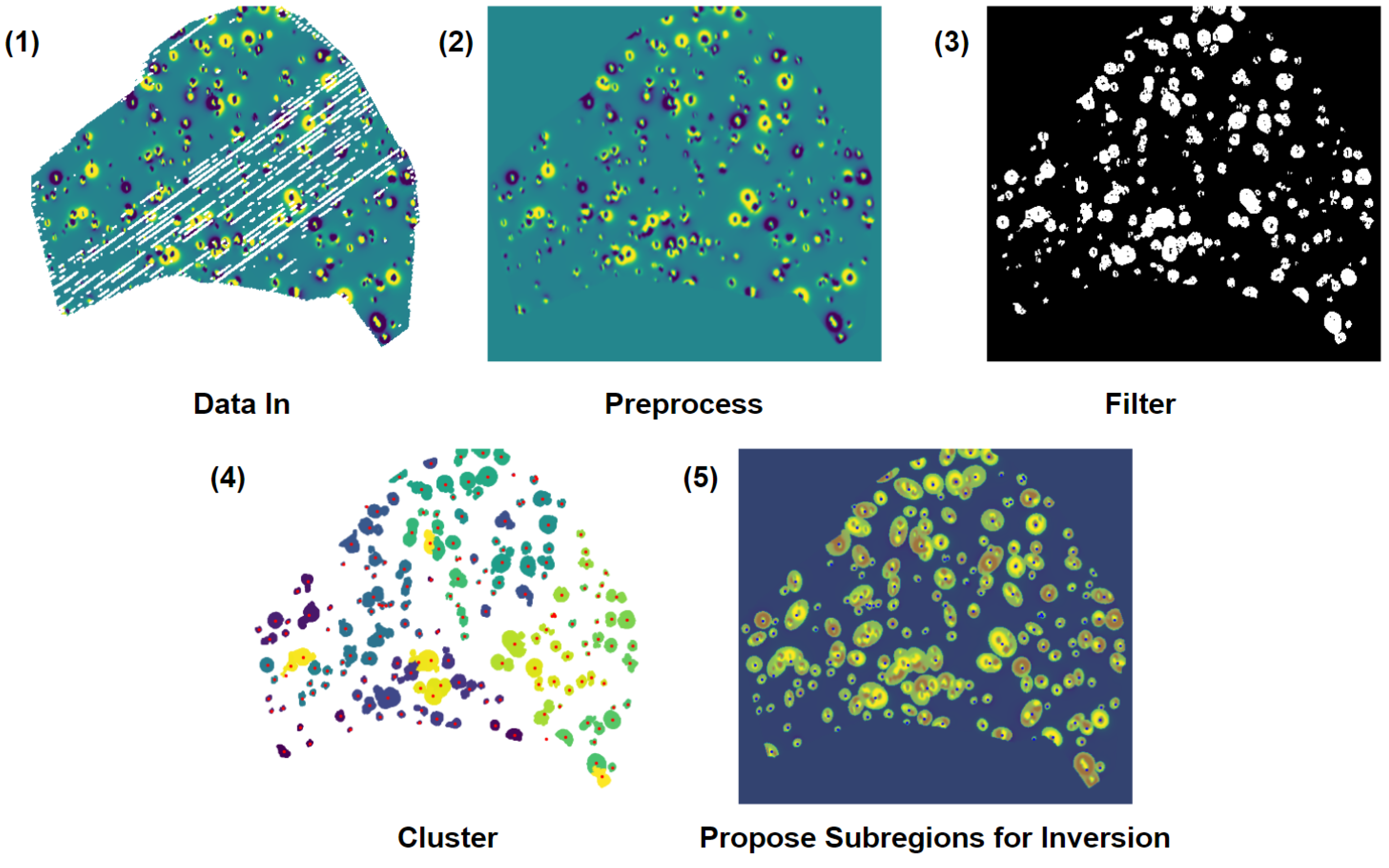
Our new method consists of four main stages, as shown in Figure 1. These stages are preprocessing, filtering, clustering, and the proposal of subregions for inversion.

In the preprocessing stage, we transform the data in each channel individually. First, we clip to the 5th and 95th percentiles to reduce the impact of outliers and the z-score. We also apply standard preprocessing such as smoothing to reduce noise, cropping boundaries to avoid unstable behavior, and compressing the image to improve processing speed.

In the filtering stage, we transform these three channels of information into a single two-dimensional binary grid. We assign a score of 1 when the magnitude of the z-score is at least $1.5$ for at least one of our three channels and 0 otherwise.

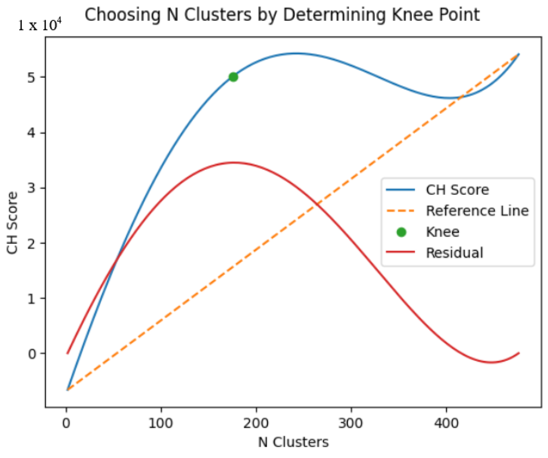
We then perform hierarchical clustering using the single distance metric on the filter’s two-dimensional binary gridded output. If the survey is large, we divide it before clustering to improve performance and then stitch the results back together. We automatically select the initial number of clusters by computing the Calinski–Harabsz (CH) score for a varying number of clusters, with the CH score knee point indicating the optimal choice [15]. The knee point is calculated by determining the point on the CH score curve with the maximum perpendicular distance from the straight line joining the first and last point on the curve (Figure 2). Large clusters are then further divided by recursively clustering using Ward’s distance metric of minimum variance until each cluster is smaller than 20 m².

Finally, we use the Khachiyan algorithm to fit the minimum area ellipse to enclose each cluster with a $1.5$ m buffer. Our proposed subregions for inversion are these ellipses, with each centroid used as the initial guess of the target’s coordinate location. Billings et al. briefly allude to using an automated masking procedure to fit ellipses to contours of anomalous regions [3]. However, not enough detail is provided to determine whether these procedures are similar.

The pipeline we described above, from data ingestion to the proposal of inversion targets, is fully automatic; we selected the hyperparameters based on our exploration of our synthetic dataset, and no human intervention is needed at any stage. This method relies on the inversion step to automatically determine the number of targets and their exact locations in each selected subregion.

Our code at github (accessed on 28 January 2024) logs the time taken for each significant part of the pipeline. In particular, the clustering algorithm uses $\mathcal{O}\left(n^2\right)$ as the number of input points, and the run time naturally increases with larger surveys, complex geology, and more targets. In order to manage this computation time when many points are to be clustered, the algorithm divides the survey into smaller subproblems for clustering and then stitches them back together. Recorded times for the computation of the linkage matrices for our surveys ranged from 17 to 113 s. End to end, the entire process took seconds for smaller surveys (around 5000 m²) and up to several minutes for more complex cases.

3. Results

We created seven synthetic surveys as discussed above. We used our new method to propose targets for inversion, and we present the results in

Table 1. Number of targets present, number of proposed inversions, and number of missed targets (false negatives) for the seven synthetically generated surveys.

Survey No.	No. of Targets	No. of Inversions	No. of False Negatives
1	277	164	0
2	175	108	0
3	182	135	0
4	150	117	0
5	348	251	0
6	292	202	0
7	269	173	0

. To score our method, we classified an anomaly as “found” if its center, defined as the center of a bounding box enclosing the anomaly, was contained within at least one area proposed for inversion. In all seven synthetic surveys, our method captured all potential targets, and due to clustering, proposed fewer inversions than targets.

In the figures below, every ellipse represents a proposed subregion with an unknown number of targets. The number and location of targets for the entire area of the ellipse will be determined downstream in the inversion step independently of any other regions. In the case of overlapping ellipses, the overlapping region will be considered multiple times in different inversion computations. In the event of one inversion resolving a target in the overlapping area but not the other, we recommend taking the more conservative result. If both inversions place a target in the same position this can be resolved as a single target.

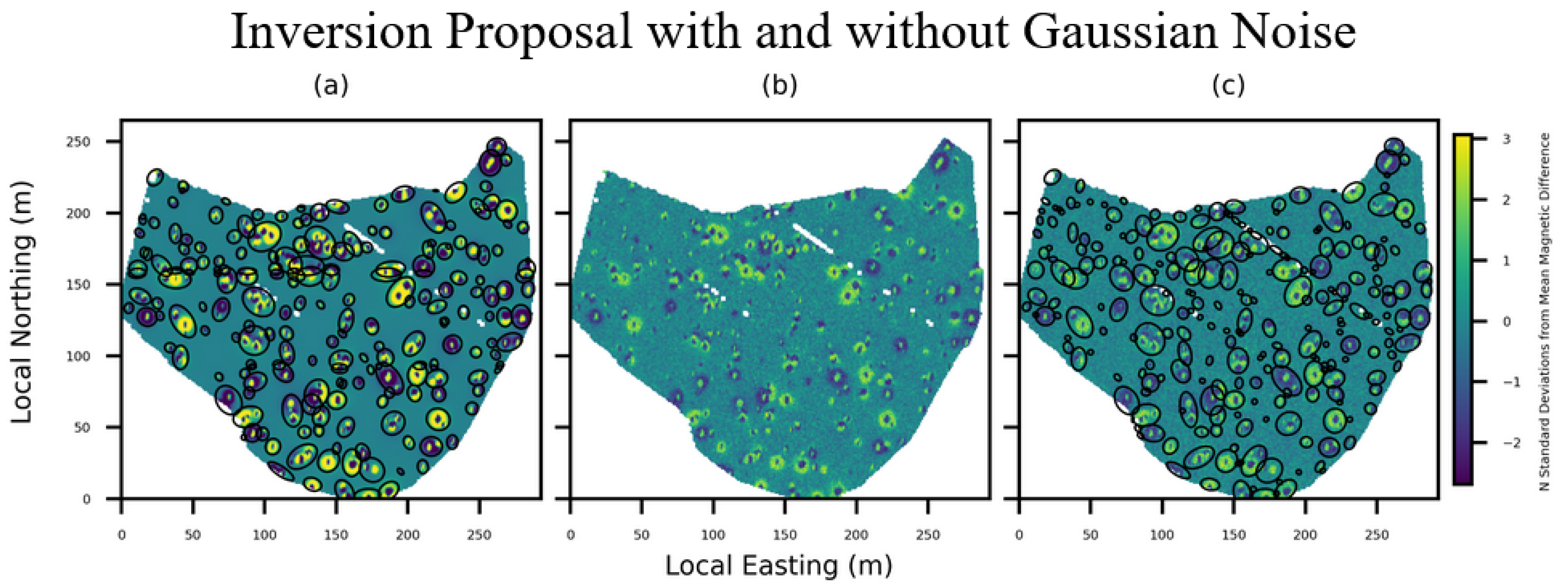
To assess the stability of our method, we performed additional experiments with Gaussian noise added to the data. Figure 3 shows our methods’ proposals on a synthetic dataset before and after the addition of noise. The number of proposed inversions increased from 164 to 225 after the addition of noisy data. All targets were still captured.

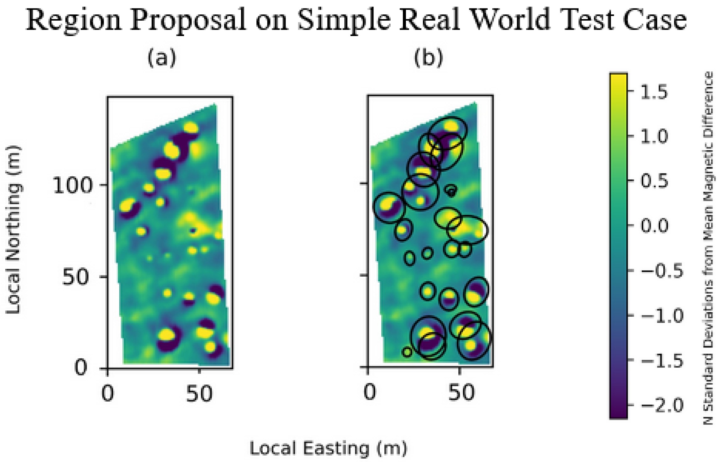
We then applied our method to a real-world dataset with a relatively clean and simple magnetic background (Figure 4). In this first real-world dataset, our method selected 22 small, well-defined subregions that covered all anomalies present (Figure 4).

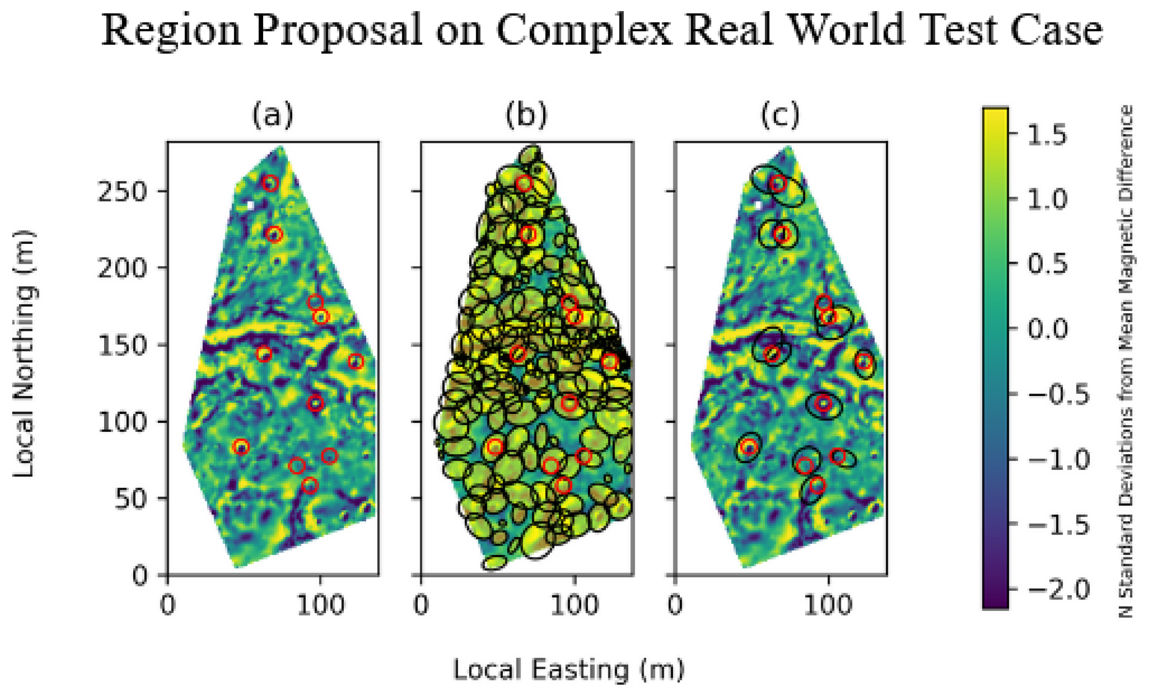
Finally, we applied our method to a real-world dataset containing complex geology that we had previously collected at a UXO detection test facility in Denmark where targets were buried at known locations. This second real-world survey contained 11 buried targets. Our method captured all 11 buried targets with 97 subregions proposed for inversion (Figure 5b). This is a substantial improvement over our previous approach, which proposed 453 inversions [14]; note that this new method provides a less sophisticated guess for the initial target position and instead relies on the inversion step to converge on the number of targets and their positions in each subregion.

4. Discussion

Both our new and previous models were able to detect all buried targets; there were no false negatives. However, our previous method proposed 453 inversion targets, while our new method captured all true positives within 97 proposed inversion areas: a decrease of over $75\%$. It is important to consider in this comparison that although our method proposes fewer inversions overall, it makes a less sophisticated guess for initial target positions and relies instead on the inversion step for precise target locations. However, this still represents a significant computational improvement for the automatic gathering of inversion priors. We also improve efficiency in the downstream inversion calculations themselves by fitting elliptical regions rather than rectangular ones; this leverages the natural shape of magnetic anomalies to minimize the selected area.

Furthermore, our method also avoids the pitfalls of some previous attempts by being robust to closely clustered targets and to noise.

Because we use a conservative, globally determined threshold, our method is robust to the possibility of multiple closely clustered targets. That is, even if multiple targets produce a locally homogeneous subregion of high readings, we still correctly identify this subregion as an area of interest to be subjected to additional scrutiny through inversion. Each subregion is taken to contain an unknown number of targets, and the method relies on the downstream inversion process to resolve the true number of targets present. This is achieved in the inversion step by attempting to fit increasing numbers of dipoles and evaluating which value provides the best fit: whether that is none, one, or multiple.

As seen in Figure 3, when we add Gaussian noise, more inversions are proposed, and the area of the proposed regions tends to increase, with most of these new proposals covering irrelevant areas. This is an interesting phenomenon that deserves some extra explanation. Whether we add noise or not, when we winsorize and normalize the data, we produce an approximately normal distribution. Then, the expected number of "points of interest" can be written in terms of $\Phi$, the cumulative distribution function of a standard normal, and should remain unchanged. However, the added noise does affect the distribution of these points of interest throughout the survey, as they are now spread further apart rather than being concentrated around, e.g., UXO or geographic features. When we perform our clustering step, we then find more numerous and less targeted clusters and thus more and larger subregions proposed for inversion. However, all target signatures within the magnetic dataset are still captured.

Most importantly, our pipeline is fully automatic from data ingestion to the proposal of areas for inversion, whereas previous attempts have needed human intervention [10].

In order to compare the performance of our new method to our previous approach, we ran our new method on the same real-world dataset previously gathered at a UXO detection test facility in Denmark [14]. This real-world survey has a complex background with prominent geological features.

Our new method reduced the number of proposed inversions by over $75\%$ while detecting all targets, which shows clear improvement. Our methods make no attempt to distinguish magnetic fields generated by geology and instead rely on the inversion step to assert if UXO is present. As seen in Figure 5, our method will propose a series of inversions along geological features. The same is true of any other object with a significant magnetic field, such as a buried pipeline. Covering these complex features with clusters may not initially seem like an improvement upon inverting the entire region. However, since the inversion calculation’s complexity is much greater than $\mathcal{O}\left(n\right)$, many smaller inversions are generally much faster to compute than a single large inversion. Dividing the survey into well-defined subregions by clusters that include complete target signatures offers a significant step towards a fully automatic pipeline for UXO detection. Furthermore, any improvements made to the data, such as reducing the prominence of geology through improved survey methods, would then directly reduce the number of subregions our method proposes.

While we could further reduce the number of false positives by increasing the z-score threshold, this is inadvisable due to the highly asymmetric costs of a false positive versus a false negative. For the same reason, our work needs to be evaluated thoroughly on more diverse real-world datasets. Thorough discussions on ethics and risk are also required when striving towards automation in the domain of UXO detection. This paper makes no attempt at any such discussions and serves simply as a proof of concept.

5. Conclusions

We proposed and implemented a novel method for the selection of subregions for inversion within UAV-collected magnetic data for the detection of UXO. This method is automatic, as no human input is required. We performed minimal hyperparameter selection of the z-score threshold and clustering objective functions using only synthetic data; using these hyperparameters, our model performed well on real-world data: capturing all true targets while also reducing the total number of subregions proposed for inversion by over $75\%$.

Our work is a proof of concept for a potential fully automatic pipeline. Future work includes increasing trust in our method by applying it to more diverse real-world data and further reducing the number of false positives through improvements in preprocessing.