Baseline Climatology of the Canary Current Upwelling System and Evolution of Sea Surface Temperature

Abstract

Global climate change has induced a rise in sea surface temperature (SST), although this increase is not uniform across the world. Significant variations exist between coastal and offshore waters, particularly in regions affected by upwelling processes. This study focuses on the Canary Current Upwelling System (CCUS), stretching from Northwest Iberia to Northwest Africa. High-resolution remotely sensed SST data (0.05°) from the ODYSSEA Level 4 Sea Surface Temperature Reprocessed dataset were validated with in situ measurements and employed to establish a regional climatological baseline for 1982–2012. Subsequent years were compared to this baseline to construct SST anomaly maps, revealing SST changes since 2012. The study area was further divided into sub-regions for comparative analysis. Results indicate that SST consistently increased at a higher rate offshore compared to the adjacent nearshore regions. A reference dataset spanning 1951–1981 was used to gauge SST variability between the two baselines. SST exhibited a 0.59 °C increase from 1951–1981 to 1982–2012, with a slowing of SST trends beyond the 1982–2012 baseline. This research offers valuable insights into the climatological dynamics of the CCUS. These findings enhance our understanding of this critical coastal system’s climatology, laying the groundwork for future investigations into evolving climate patterns in coastal regions.

1. Introduction

The oceans play a fundamental role in Earth’s climate system. Due to their large heat capacity, they display a characteristically long timescale, which further leaves a marked signature on atmospheric circulation [1]. As the sea surface separates the ocean from the atmosphere, sea surface temperature (SST) is a fundamental parameter in understanding the interaction between the two and their influence on each other. Any changes in ocean–atmosphere heat exchange create large-scale and long-lasting SST anomalies [1]. Global climate change has led to a rise in sea surface temperature (SST) throughout the world’s oceans. Monitoring changes in SST is crucial considering oceans cover 70% of the Earth’s surface [2]. According to the most recent report from the Intergovernmental Panel on Climate Change (IPCC), the rate of warming is higher near the surface of the ocean, where SST increased by more than 0.1 °C per decade from 1971 to 2010 [3]. This should be a concern considering that changes in SST directly impact coastal ecosystems around the world [4]. The rate of warming is not uniform throughout the global oceans [5] and major differences have been observed between coastal waters and offshore waters [4,6]. A study by Lima and Wethey [4] found higher decadal rates of SST change in coastal waters compared to the global ocean based on remotely sensed SST data. Those authors further found higher increases in coastal SST in locations between the Tropic of Cancer and the Arctic Circle [4].

SST differences between coastal and offshore waters can be seen in regions where upwelling occurs: a phenomenon in which surface water is transported offshore due to the combined effects of both wind and the Coriolis force, and replaced with cold nutrient-rich water from below [7]. In Eastern Boundary Upwelling Systems, upwelling occurs due to northerly winds blowing towards the equator, forcing an Ekman transport of water offshore. There are four major Eastern Boundary Upwelling Systems in the world: the Canary current system, the Benguela current system, the Peru (also known as the Humboldt) current system, and the California current system [7]. Lima and Wethey [4] found decreases in SST in the California and Humboldt currents, but increases in SST in the areas of the Canary current and Benguela current.

Due to their high nutrient content, upwelling regions are highly productive for marine ecosystems, aquaculture, and fisheries [8,9,10]. Changes in climate will have an impact on upwelling areas as changes in windspeed and direction govern this phenomenon.

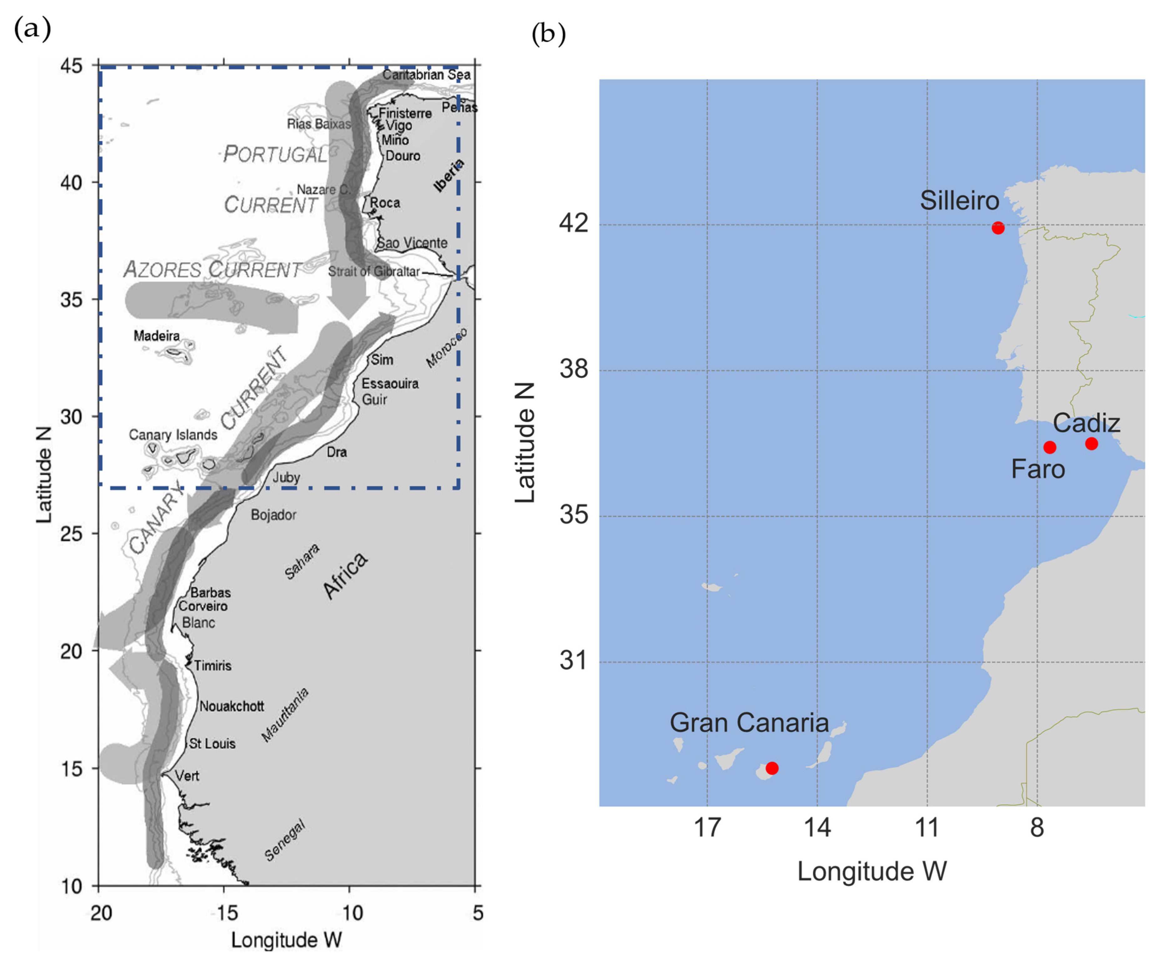
The focus of this study is the Canary Current Upwelling system (CCUS). This extends from 43°N off the coast of Iberia to 10°N off the coast of Senegal (Figure 1a), which is approximately the range of displacement of the Trade wind band. The continuity of this upwelling region is interrupted by the Strait of Gibraltar, which allows the exchange of water between the Mediterranean Sea and the Atlantic Ocean. The circulation off the coast of Iberia has been classified as the Portugal Current System [11] The weak Portugal Current flows southward year-round along the oceanic side of the Iberian Peninsula. The circulation pattern is more complex at the ocean margin, with seasonal variability caused by coastal winds. During spring and summer, the northeasterly winds produce the southward-flowing Portugal Coastal Current at the surface and the northward-flowing Portugal Coastal Undercurrent at the slope [12]. During autumn and winter, southwesterly winds provoke a reversal of the surface circulation to form the Portugal Coastal Counter Current, which flows northward from the surface to 1500 m depth, including the propagation of the Mediterranean Overflow Water along the western and northern Iberian slope. The seasonal upwelling and downwelling periods vary strongly from year to year, describing a decadal cycle linked to the North Atlantic Oscillation (NAO) [13]. Successions of upwelling and relaxation events occur over a period of 1–3 weeks [14,15]. Northerly winds produce upwelling off the western coast, whereas easterly winds produce upwelling off the northern coast. The orientation of the coast changes abruptly north of Cape Finisterre, making both northerly and easterly winds favorable at this location. Similar considerations apply to Cape São Vicente and the coast of southern Portugal, now with westerly winds producing upwelling off the southern coast [16]. The coastal upwelling region from Gibraltar to Cape Blanc is maintained by northeasterly winds throughout the year, with more intense winds and upwelling during the summer months [17]. The upwelling between Cape Blanc and Cape Vert has a seasonal peak during winter. The northwest African coast is largely influenced by the North Atlantic subtropical gyre’s general circulation, particularly, the “Canary Current.”

The Canary Current flows equatorward while interacting with coastal upwelling waters and detaches from the coast near Cape Blanc, flowing westward at the latitude of Cape Vert. Arístegui et al. [17] have confirmed water inflow from the open ocean into the coastal upwelling region north of the Canary Islands. A study on the Canary Coastal Transition Zone (CTZ) regions’ coupling between coastal and open ocean waters has found that water recirculates south along the continental slope, where quasi-permanent filaments stretch offshore and exchange water properties with island eddies [18]. Flow reversals in the main flow have been observed close to the upwelling-CTZ during late fall and winter, allowing the offshore spread of organic matter produced in upwelling waters near the Canary Islands region [19]. Two cells transport upwelled waters into the open ocean: the standard vertical cell and the horizontal circulation cell originate from the impinging of open ocean water north of Cape Guir, which is closed by the offshore export of water through several upwelling filaments and the flow diversion at Cape Guir. The upwelling region is a key region for the export of organic matter and nutrients in the open ocean [17].

Changes in climate are hypothesized to intensify upwelling favorable winds since the winds are a result of a strong atmospheric pressure gradient between a thermal low-pressure cell over a heated landmass and higher-barometric-pressure cell over a cooler ocean [7]. With CO₂ levels rising over the past several decades, daytime heating over landmasses has increased more than it has over the ocean, further enhancing the land–sea pressure gradient that drives nearshore upwelling [7]. As upwelling regions account for 20% of the global fish catch [20], it is crucial to study the long-term trends of these regions that are highly sensitive to climate change. Another consequence of climate change for coastal upwelling systems is the displacement of these systems northward [21].

Several studies have characterized the CCUS based on historical data [13,22,23] and one recent study has evaluated the future evolution of the system based on the rate of global warming given by the Intergovernmental Panel on Climate Change (IPCC) [21]. However, there is a lack of agreement on the conclusions of these studies due to the different analyses and approaches in detecting long-term trends and the interannual variability of SST in the region [24]. Furthermore, there is a gap in the literature comparing recent SST changes, specifically off the coast of Iberia, and comparing them to a baseline. The CCUS region has not been extensively studied with regard to SST trends. Previous studies that have examined these trends have mostly relied on remotely sensed SST data with a low spatial resolution. However, given that upwelling can only be detected near the coast, it is imperative to use satellite data with a fine spatial resolution [4]. A recent study has compared remotely sensed SST data with a resolution of 0.25° to climate models and has found that the rate of warming in coastal waters is slower than that in adjacent offshore waters [21]. This finding differs from that of Lima and Wethey [4], highlighting the importance of updating research findings and utilizing satellite data with fine resolutions to draw conclusions about SST rates of change.

Human-induced global warming and natural variations from year to year and decade to decade shape our climate. Climatologists, including those at the Copernicus Climate Change Service (C3S), use standard reference periods to create average ‘climate normals’ that represent a typical climate for a period based on the World Meteorological Organization’s (WMO) definition. The WMO defines a climate normal as the mean of climatological data over a period of at least three consecutive ten-year periods [25]. These climate normals are used to compare short-term data at local, national, or global levels. In 2015, the WMO’s decision-making body on standards, the World Meteorological Congress, approved a resolution to update the climatological Standard Normals every ten years to keep them relevant in a rapidly changing climate. The WMO used 1981–2010 as the base period for operational purposes, while retaining the 1951–1981 dataset [26] as the historical base period for supporting long-term climate change assessments. The two-tier approach was intended to harmonize and standardize the differing national approaches and facilitate international comparisons. Different researchers and weather services use different baselines, resulting in inconsistent comparisons, but the new technical regulation on “Calculating Climatological Standard Normals” [25] means that all countries will start using the period 1981–2010, updated every ten years. The 30-year climate normal to be used in the 2020s will be 1991–2020, while the 1951–1981 baseline for assessing climate change will be kept until there is a scientifically compelling reason for changing. As a result, in Europe, C3S started to use the 1991–2020 climate normal as the main reference period for monthly climate bulletins from January 2021 onward.

The aim of this work is to understand the recent evolution of SST in the CCUS by assessing SST interannual variability based on the WMO and C3S guidelines. Changes in SST in the CCUS can have significant impacts on fisheries, particularly those producing small pelagic species such as sardines and horse mackerel. Long-term changes in alongshore winds in the Iberian Peninsula have been linked to variations in upwelling patterns and decadal fluctuations in the annual catch of sardines, with sustained and intermittent northerly winds during the winter spawning season having a negative impact on recruitment and catches the following year [27,28]. South of 36°N, the relationship between recruitment variability and the environment is not well understood due to a lack of adequate data, but several patterns have been documented [29,30]. A comparative analysis of spawning patterns in the Canary Current has shown that the timing of spawning for small pelagic species such as sardines and sardinellas is associated with the occurrence of wind speeds of about 5–6 m/s, which corresponds to the optimal wind conditions for recruitment success [29,31]. This suggests that small pelagic fish have adapted their reproductive strategies to the environment over the long term. Changes in SST can also have significant impacts on the aquaculture industry, affecting the growth and survival of farmed fish and other aquatic organisms. One of the most immediate effects of SST change is changes in the timing and duration of the growing season for aquaculture species. In some cases, warmer temperatures may result in earlier or extended growing seasons, allowing farmers to produce more fish in a given year. However, in other cases, changes in temperature may result in shorter growing seasons, reduced growth rates, and lower survival rates for fish, ultimately reducing production and profitability [32]. Changes in temperature can also affect the prevalence and severity of disease in aquaculture systems. Warmer temperatures can increase the incidence rate of certain diseases, as well as the growth and virulence of some pathogens, while simultaneously reducing the immune response of fish and other organisms [33]. It is therefore important to continue monitoring changes in SST and their effects on marine ecosystems to better understand and prepare for these impacts [34,35].

This study aims to analyze SST trends from 1950 to 2020 based on SST data from high-resolution satellite measurements. The article is structured as follows: Section 2 describes the satellite SST dataset used in this study and the process of validating this product with in situ observations. The section further describes the criteria used in determining the regions used for nearshore/offshore analysis. The computations for the various baselines and SST anomalies are also described. Section 3 presents and discusses the results of (1) the validation of the satellite product, (2) the climatological normal SST for the 1982–2012 baseline period, (3) yearly anomalies from the 1982–2012 baseline period, (4) an analysis of the areas that showed significant warming and cooling, (5) time series analyses to compare the various baselines as well as show the interannual variability, and (6) the SST anomaly between the 1982–2012 baseline and the 1991–2020 baseline. Section 4 discusses the major findings of this work as well as suggestions for future work.

2. Materials and Methods

SST data were obtained from the Copernicus Marine Environmental Monitoring Service (CMEMS). The ocean product selected for this study was the ODYSSEA Level 4 Sea Surface Temperature Reprocessed over the European North West Shelf/Iberia Biscay Irish Seas. This product was processed by IFREMER (French Research Institute for Exploitation of the Sea) and included SST fields that had been reconstructed from the European Space Agency Sea Surface Temperature Climate Change Initiative (ESA SST CCI) L3 products from 1982 to 2016 and from the Copernicus Climate Change Service (C3S) L3 product from 2016 to 2020 [36]. The SST data in this dataset were derived from satellite thermal infrared measurements from 11 advanced very-high-resolution radiometers (AVHRRs) and 3 along-track scanning radiometers (ATSRs). Only nighttime observations and those with a good quality were included in the analysis for reconstructing the SST field. The satellite local overpass time varies between satellite missions and can also drift during a mission [37]. Thus, the mean SST was computed based on the results of the various satellite passing times. As previously mentioned, only nighttime observations were used to exclude the effects of diurnal warming. The final result of the product was a daily gap-free SST field from 1982 to 2020 with a spatial resolution of 0.05°, representing SST at a depth of 20 cm [36].

The spatial coverage of the grid window used in this study was 27°N to 46°N and 20°W to 5°W, covering the upwelling system off the coast of Iberia and off the northwest coast of Africa.

The satellite product had previously been quality-checked and was validated at IFREMER with drifting buoy measurements as recommended by the GHRSST group for SST validation (STVAL) [36]. The differences between the satellite product and in situ observations were computed by bi-linear interpolation of the analysis to the in situ locations for that day. The mean and standard deviation were then averaged, resulting in a mean value of −0.06 K and standard deviation of 0.46 K [36].

Since the previous validation results only came from drifting buoy measurements, an additional mooring buoy product was considered to further assess the quality of the satellite product. Mooring buoys are anchored and provide point measurements of temperature at specific locations. Comparing satellite SST data with data from mooring buoys can provide validation and calibration of the satellite data, ensuring its accuracy and reliability. Mooring buoys are typically equipped with high-precision temperature sensors that provide accurate measurements of water temperature at various depths, whereas satellite SST data are derived from remotely sensed measurements that may be subject to various errors and uncertainties. By comparing the two datasets, any discrepancies or systematic errors in the satellite data can be quantified.

To assess the satellite SST dataset, data from four mooring buoy stations, distributed along the study area, were used to validate the satellite product with in situ observations. Hourly buoy data from the following stations were used: Gran Canaria, Faro, Gulf of Cadiz, and Cabo Silleiro (Figure 1b). The buoy datasets of Gran Canaria, the Gulf of Cadiz, and Cabo Silleiro contain SST measurements from 2001 to 2020, whereas the Faro buoy dataset contains data only from 2016 to 2021.

Since each buoy dataset contains SST observations every hour, the daily average, minimum, maximum, 10th and 90th percentiles were also computed to gain a complete understanding and analysis of the daily SST values at each station.

To compare the satellite observations with in situ measurements, both qualitative and quantitative assessments were performed between the two datasets. For simple quantitative comparisons between the two datasets the following error metrics were computed: root-mean-square error (RMSE) and BIAS. For a more elaborate quantitative assessment to evaluate the level of agreement between the two datasets, the model skill score (MSS) was computed.

The first error metric, RMSE, is an absolute measure of how much the satellite data deviate from the in situ buoy measurements [38]. More specifically, it is the standard deviation of the distribution of the differences between the satellite observations and the in situ observations. It is represented by the following equation:

$$RMSE=\sqrt{\frac{\sum _{i=1}^n{\left(x_{RS}-x_{insitu}\right)}^2}{n}}$$

(1)

where $x_{RS}$ and $x_{insitu}$ refer to the remotely sensed data and in situ buoy data, respectively. $n$ is the number of observations. Since the satellite data consist of one mean SST value for each day and the buoy data contain hourly measurements for each day, the buoy data were averaged to obtain the mean SST value for each day at the satellite passage time. To be consistent with the nighttime observations from the satellite, only nighttime observations of the buoy data were considered in this analysis. Therefore, the buoy data were resampled to obtain one nightly SST value that was averaged between the hours of 10 p.m. and 6 a.m. Furthermore, any dates that contained missing values were also removed when computing the error differences. Thus, for the computation of the error metrics, the number of buoy observations is equivalent to the number of satellite observations.

The BIAS also provides an absolute measurement of the error between the satellite data and buoy data. In this case, it is the average difference between the remotely sensed observations and the in situ observations. It is represented by the following equation:

$$BIAS=\frac{{\sum }_{i=1}^n{\left(x_{RS}-x_{insitu}\right)}_{ }}{n}$$

(2)

The model skill score (MSS) is a value proposed by Willmott [39] that overcomes the sensitivity of correlation statistics to differences in the predicted mean and variances [38]. It is represented by the following equation:

$$MSS=1-\frac{{\sum }_{i=1}^n{\left(x_{RS}-x_{insitu}\right)}^2 }{{\sum }_{i=1}^n{\left(\left|x_{RS}-{\overline{x}}_{insitu}\right|+\left|x_{insitu}-{\overline{x}}_{insitu}\right|\right)}^2}$$

(3)

${\overline{x}}_{insitu}$ represents the mean value of the buoy dataset. The MSS can range from anywhere between 0 and 1, with a value of 1 indicating perfect agreement between the two datasets, whereas a value of 0 represents complete disagreement between the two datasets.

To understand its recent SST evolution in the CCUS, the definition of a climatological standard normal, defined by the World Meteorological Congress (WMO) as the average of climatological data computed for a consecutive period of 30 years [25], was used to derive two climatological normals (baselines) from the satellite dataset: (1) for the interval [1982–2012] and (2) for the interval [1991–2020]. These normals were defined based on the WMO and C3S guidelines for the available satellite dataset interval. For both periods, the average SST was computed over the entire 30-year period, as well as for each monthly and seasonal average. Seasonal climate normals were computed considering Winter, meaning January, February, and March (JFM); Spring, meaning April, May, and June (AMJ); Summer, meaning July, August, and September (JAS); and Fall, meaning October, November, and December (OND).

Anomalies were then computed to evaluate the variability in SST with consideration of the two baselines defined. This was conducted by subtracting the baseline SST values from the SST values of each year. It is represented by the following equation:

$${SST}_{anomaly}={SST}_{value}-{SST}_{baseline}$$

(4)

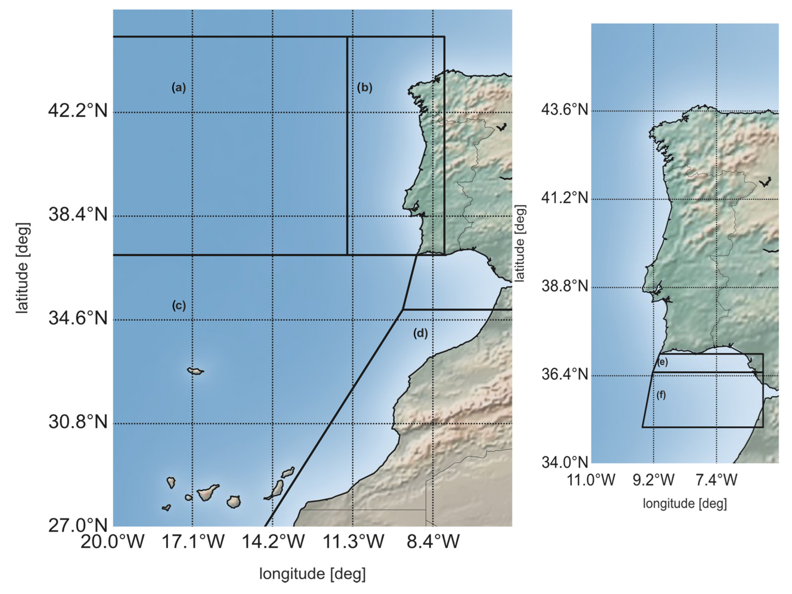
This analysis was performed for a monthly, yearly, and seasonal timescale as described above. The standard deviation of each anomaly map was also computed to assess how much each geographical cell deviated from the entire mean of the study area. To assess the SST evolution in key oceanographic components of the CCUS, the study area was divided into six regions (as shown in Figure 2). The division of the study area into six distinct regions was driven by the significance of these areas within the context of CCUS climatology. Each of these regions plays a crucial role in the oceanographic dynamics of the CCUS domain, thereby warranting detailed investigation. The rationale for considering these regions as critical can be elucidated as follows:

(a)

Offshore off the coast of West Iberia: This region is crucial for understanding the continuation of the Portugal Current System’s influence on the West Iberian margin. This area is characterized by the presence of oceanic features and frontal structures that contribute to SST variability and broader climate trends.

(b)

Nearshore off the coast of West Iberia: This region is essential for exploring the coastal interactions within the West Iberian margin. Coastal SST patterns here are influenced by a combination of factors, including the interaction between continental shelf dynamics, local upwelling, and overall circulation patterns.

(c)

Offshore off the coast of northwest Africa: The offshore waters adjacent to northwest Africa are vital as they represent the extension of the Canary current system. These waters are characterized by the influence of major oceanic currents and fronts, making them integral to understanding broader regional climate dynamics and the transport of heat and nutrients.

(d)

Nearshore off the coast of northwest Africa: This region is critical due to its proximity to the African continent and its interaction with prevailing oceanic currents and atmospheric processes. The nearshore area serves as a transition zone between continental and open ocean conditions, where coastal upwelling and other localized phenomena can exert a significant influence on SST patterns.

(e)

Nearshore off the coast of SW Iberia: This coastal sector along the SW Iberian coast assumes paramount importance due to its intimate connection with the establishment of the Coastal Countercurrent. This countercurrent materializes as a direct consequence of the relaxation of upwelling-favorable winds and the consequential pressure gradient along the coastal margin. This dynamic feature gives rise to a discernible flow of water masses, which significantly influences the local SST patterns. The intricate interplay between the Coastal Countercurrent and prevailing oceanic and atmospheric forces necessitates thorough investigation of this region’s SST trends.

(f)

Offshore off the coast of SW Iberia: In the broader context of regional oceanography, this offshore expanse adjoining the SW Iberian coast holds particular significance. Here, the interactions between the Coastal Countercurrent and adjacent oceanic currents come into play, further shaping the local hydrographic and thermal characteristics. The offshore region displays the interplay between the Coastal Countercurrent and the broader-scale circulation patterns that generate distinctive SST variations. Consequently, understanding the complexities of this interaction is crucial for unraveling the intricacies of SW Iberian coastal oceanography.

By examining SST trends in these specific areas, the study aims to capture the nuanced interplay between various oceanic and atmospheric drivers that collectively shape the climatic characteristics of the CCUS. For each region, a yearly, monthly, and seasonal average was computed and compared with the normals obtained for that same region. Nonetheless, to enable historical comparisons and to monitor climate change, the WMO advises maintaining the utilization of the 1951–1981 period as a constant and standardized reference period for computing and monitoring global climate anomalies. The 1951–1981 baseline was used to evaluate the effects of climate change on the SST variability computed from the satellite dataset. This monthly dataset was constructed on a 2° × 2° grid box and includes long term monthly means [26]. The Extended Reconstructed Sea Surface Temperature (ERSST) dataset was derived from the International Comprehensive Ocean-Atmosphere Dataset (ICOADS). The entire dataset consisted of an SST analysis from January 1854 until the present. SST data came from Argo floats as well as the Hadley Centre Ice-SST version 2 (HadISST2) ice concentration [26].

3. Results and Discussion

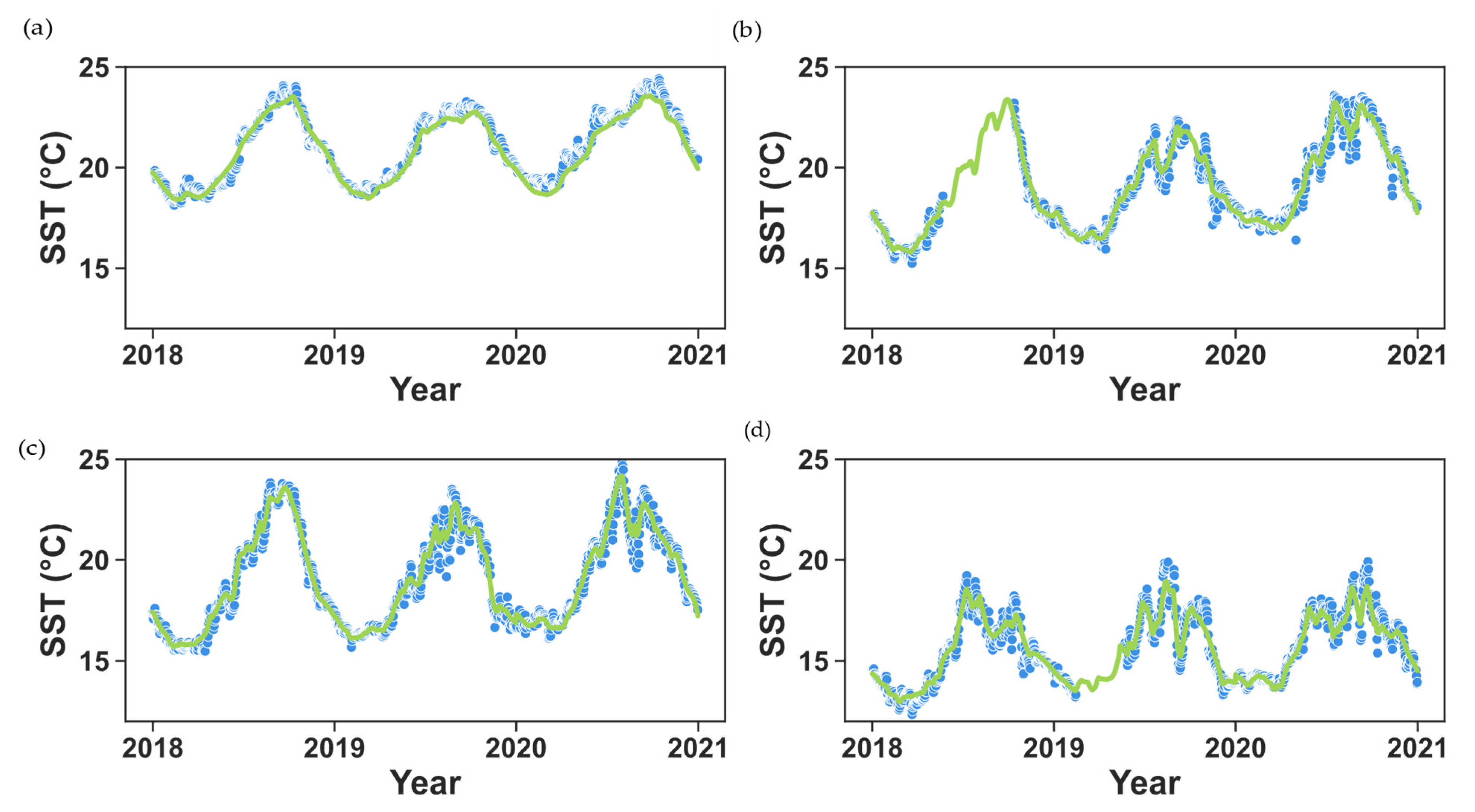
To validate the accuracy of the satellite-derived SST data, time series were constructed at four distinct locations within the study area, and these were compared with observations from the mooring buoys referred to in the last section. The comparison results are illustrated in Figure 3. The period of this analysis spanned from 2018 to the end of 2020 due to the minimal data gaps observed during this period at each mooring buoy station.

For a more precise quantitative evaluation of the differences between the two datasets,

Table 1. Table of error metrics (RMSE, BIAS and MSS) comparing the buoy datasets with the satellite datasets.

	Comparison Period	RMSE (°C)	BIAS (°C)	MSS
Gran Canaria	2001–2020	0.388	−0.200	0.969
Faro	2016–2020	0.333	0.021	0.984
Gulf of Cadiz	2001–2020	0.400	0.080	0.981
Cabo Silleiro	2001–2020	0.439	0.059	0.959

outlines the error metrics computed based on the indicators referred to in the methodology section. These results span the entire period available in each dataset, providing a comprehensive assessment of the correspondence between the satellite-derived SST data and the mooring buoy observations.

The satellite dataset used in this study serves as a good indicator for assessing SST variability in the Canary Current Upwelling System. The time series graphs comparing the satellite product with data obtained from the mooring buoys, as shown in Figure 3, demonstrate minimal disparity between the two datasets at each respective location. This alignment underscores the reliability of the satellite-derived data for monitoring SST.

RMSE values, representing the average magnitude of differences between satellite-derived SST data and mooring buoy observations, serve as indicators of the precision of satellite measurements. Across all locations, the RMSE values ranged from approximately 0.333 to 0.439 °C. These values indicate a relatively low level of error, suggesting a favorable alignment between the datasets. The BIAS values, denoting the average differences between the two datasets, help to gauge the presence of any systematic deviation. The BIAS values in the range of 0.021 to 0.080 °C reveal that the satellite-derived SST data generally exhibit minimal systematic discrepancies compared to the mooring buoy observations. The only outlier here is Gran Canaria, where the average difference between the satellite data and buoy data is the largest in magnitude with a BIAS value of −0.200 °C. Upon careful inspection of these two datasets, we found that in the year 2014 the SST values obtained from in situ measurements were significantly higher than those obtained from the satellite data, with daily differences of more than 1 °C between the two datasets. This is further attributed to the negative value in the BIAS, as the BIAS value indicates how much the buoy data deviate from the satellite data. The discrepancy between these two datasets can be attributed to the complexity of the wind and water circulation around Gran Canaria. A wind-sheltered feature around Gran Canaria, where large differences in windspeeds have been observed at distances of approximately 2 km, affects the local hydrography of this area [40]. The SST product has a spatial resolution of 0.05° (5 km), and so it cannot detect some of the smaller features in the water circulation. Additionally, considering the reanalysis-based nature of the SST product used, the differences could be exacerbated by the inherent characteristics of reanalysis data. Reanalysis products integrate various data sources, including satellite observations, through complex modeling to provide a consistent, long-term view. This process can smooth out local variations and may not accurately capture small-scale, localized phenomena, particularly in coastal regions with dynamic conditions such as those in Gran Canaria.

MSS, a measure proposed by Willmott [39] that factors in both mean and variance differences, furnishes a comprehensive assessment of the agreement between the two datasets. MSS values, being notably high across all locations (ranging from 0.959 to 0.984), underscore the robustness of the satellite-derived data in replicating the observed SST variations captured by the mooring buoys.

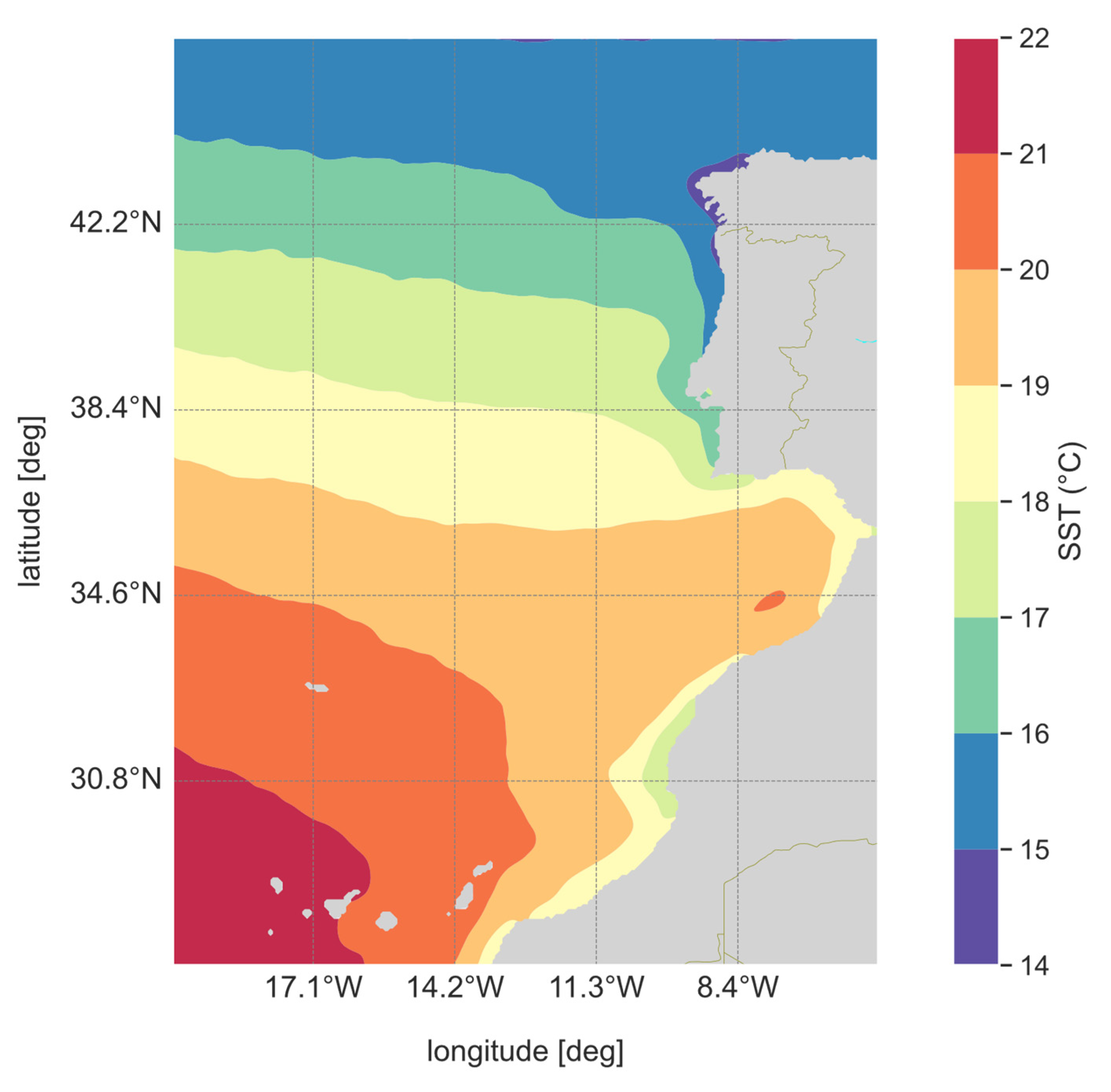
Figure 4 represents the mean climatological normal SST for the baseline period of 1982–2012 across the entire study area. It serves as an illustrative representation of the computed climatological baseline spanning the years 1982–2012. As expected, our observation reveals a compelling trend: coastal zones that are particularly susceptible to upwelling phenomena exhibit pronounced lower SST values when compared with their offshore counterparts. This differential temperature response is particularly discernible below the 42°N latitude where the Azores current exerts its presence. The local circulation dynamics off the coast of SW Iberia do not inherently encompass the presence of upwelling. However, the recirculation phenomenon of the upwelling jet originating from the West Iberian coast plays a pivotal role in shaping the SST landscape. This influence introduces a distinct SST signature in the SW Iberian coast, setting it apart from the relatively warmer waters found within the Gulf of Cadiz. This dynamic interaction contributes to the unique oceanographic tapestry that characterizes the SW Iberian coastal region. These results are consistent with other findings on the spatial distribution of SST in this region during this time period [21].

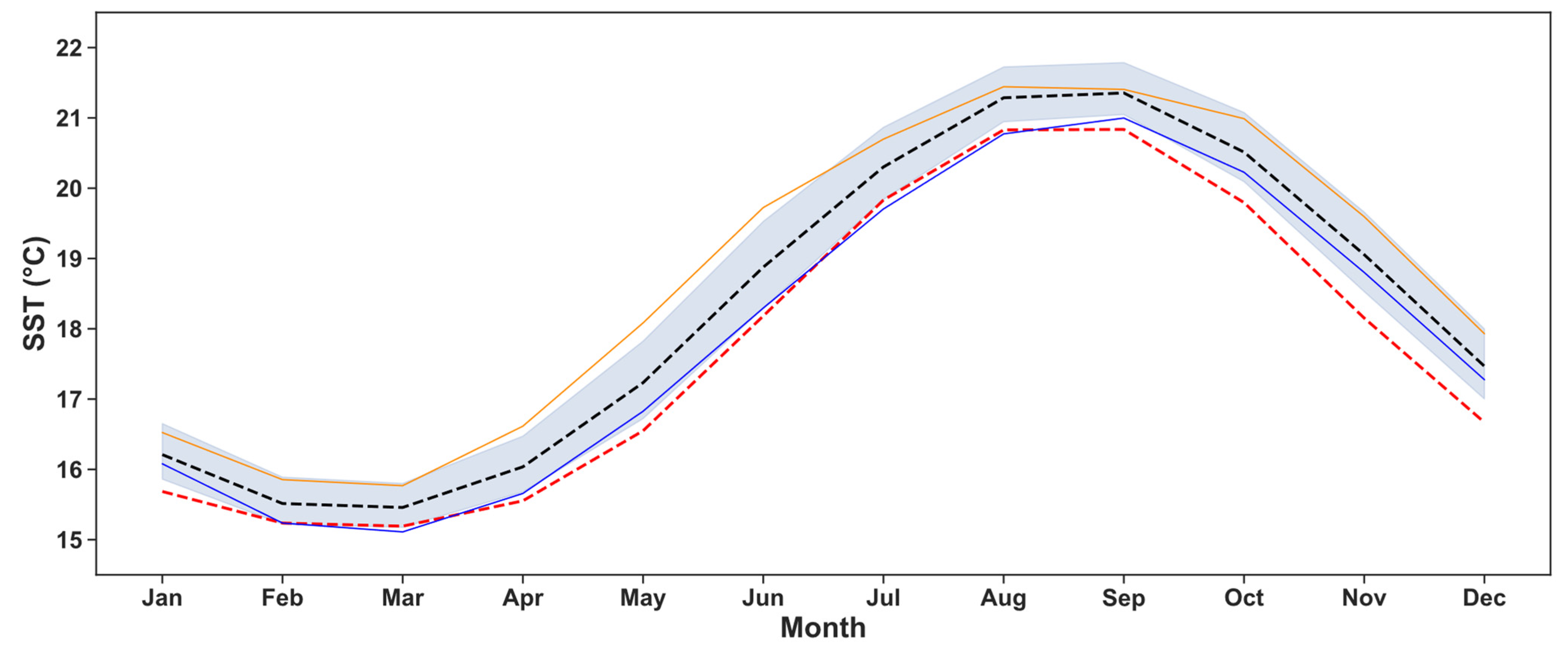
To facilitate a comprehensive overview of the monthly mean trends, Figure 5 shows the monthly mean values over the baseline period from 1982 to 2012 and the preceding historical baseline period from 1951 to 1981. Furthermore, the time series graph captures the 95% confidence interval of the monthly mean SST values from 1982 until 2021, enabling a comparison of the full dataset with each baseline. Analyzing the interannual variability, the time series graph presented in Figure 5 unveils a distinctive regional natural pattern in SST. This pattern is characterized by a consistent trend: a decline in SST from September to March, followed by a subsequent increase from March to September. This cyclic behavior persists across the various climatological periods under consideration. Furthermore, a compelling insight emerges when contrasting the climatology of the years 1982 to 2012 with that of 1951 to 1981. Overall, the 1982 to 2012 30-year climatological mean is 0.59 °C higher than the 1951 to 1981 30-year climatological mean. Throughout the year, the former consistently exhibits higher SST values compared to the latter. An intriguing observation is also found when comparing the 1951–1981 climatology (shown in red) with the entire dataset from 1982 to 2021 (shaded region). The 1951–1981 climatological mean coincides with the coldest year (as depicted by the solid blue line) in the 1982–2021 dataset, apart from the spring (AMJ) and autumn (OND) months when SST for the coldest year is higher than the SST of the 1951–1981 baseline period.

This comparison underscores that the most pronounced disparities manifest during the spring (AMJ) and autumn (OND) seasons. This trend is discovered even when delving into the analysis of the warmest and coldest years across the dataset. Remarkably, the warmest year on record (2017) with a yearly mean SST of 18.72 °C (represented by the orange line in Figure 5) demonstrates the most substantial difference in SST when compared to the remaining records. This difference becomes particularly pronounced during the spring and autumn months when the mean SST is 18.14 °C and 19.50 °C, respectively. Examining the year with the coldest SST on record (1986, with a mean of SST of 17.92 °C) we also see a stark contrast between spring and autumn, with a mean SST of 16.93 °C during spring and 18.77 °C during autumn.

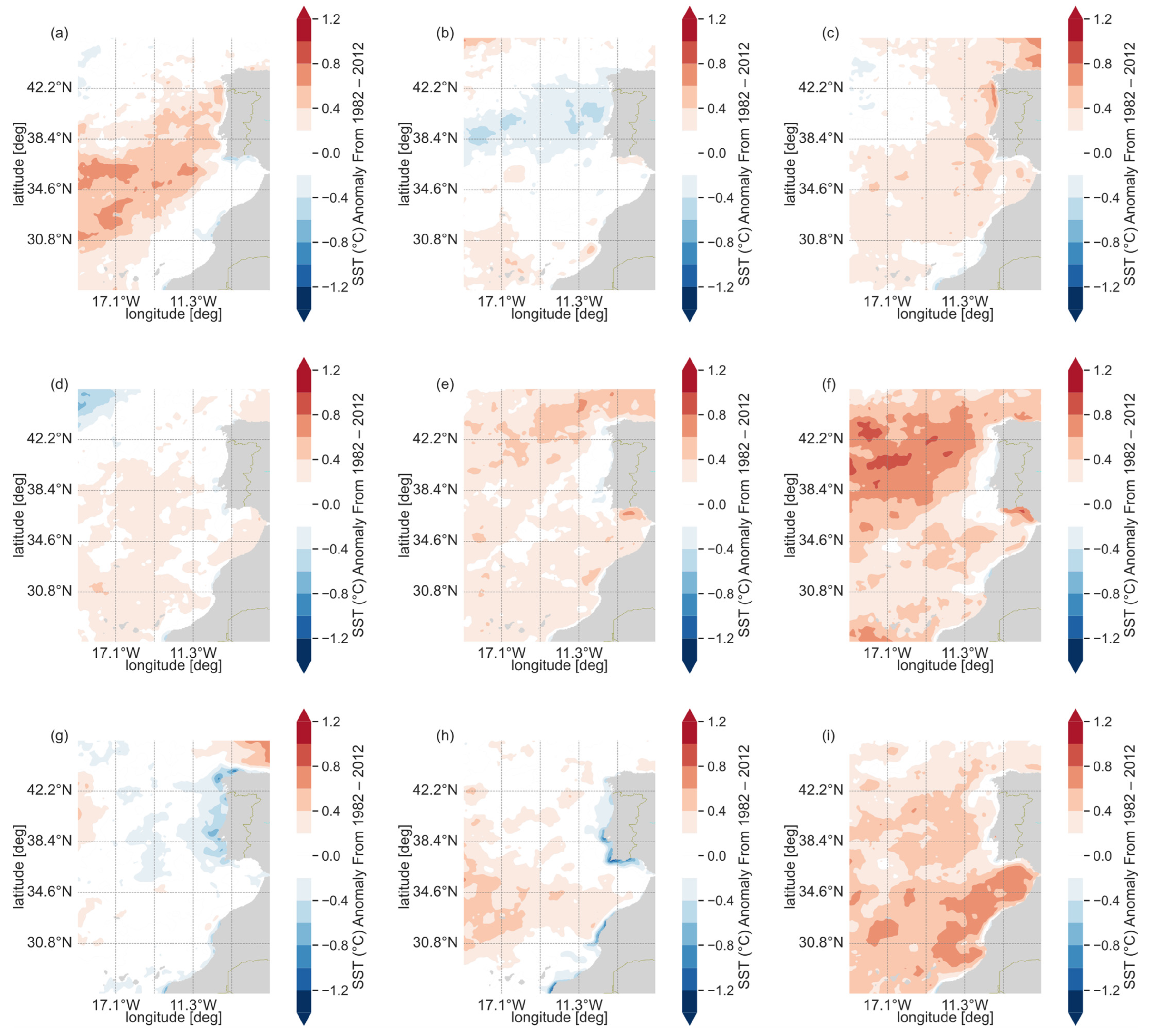
To track the temporal evolution of changes after the 1982–2012 baseline period, we generated anomaly maps by subtracting the baseline mean from each year’s dataset, starting from 2012. This analysis was conducted across yearly, monthly, and seasonal timeframes. The resulting yearly anomaly maps are depicted in Figure 6. In these maps, regions colored in red indicate instances where the SST anomaly (measured in °C) surpasses the positive standard deviation, while blue regions signify SST anomalies falling below the negative standard deviation. White areas represent SST anomalies that fall within the range of the negative and positive standard deviations. Consequently, the red cells highlight regions that have experienced warming trends since the baseline period, the blue cells correspond to areas exhibiting cooling trends since the baseline period, and the white cells indicate regions with negligible changes. The anomaly maps of Figure 6 show more red areas, corresponding with an SST increase offshore, while areas around the coastline remain white or blue, corresponding to decreases in SST compared to the 1982–2012 baseline. The years 2013 and 2018 are exceptions to this trend, and each of these anomaly maps show a decrease or no significant change in SST. The anomaly maps reveal much variability in terms of the rates of SST change and where SST is increasing or decreasing. Nearly all SST yearly anomaly maps show slower rates of SST change nearshore off the coasts of Western Iberia and western Africa. The offshore regions adjacent to these areas show much higher positive anomalies and thus higher rates of SST increase. However, areas around the coastline depict negative anomalies, and thus decreases in SST compared to the baseline. In these upwelling regions where cold nutrient-rich water is upwelled from the bottom, SST is increases at a slower rate. For several years after the end of the 1982–2012 baseline period, SST off the coast decreased. Similar results were also found by Varela et al. [21], who used climate models to evaluate SST trends in the Canary Current Upwelling System.

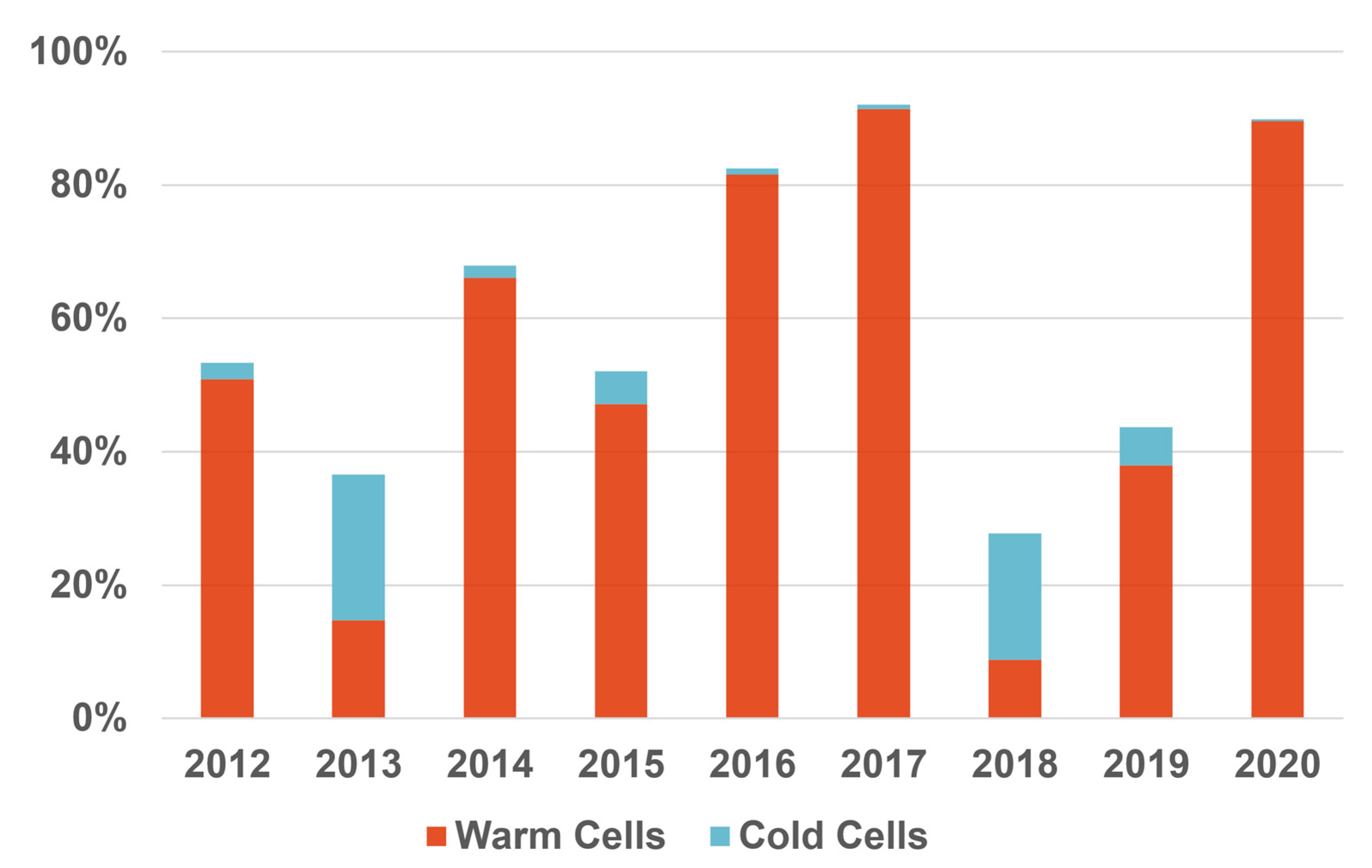
While Figure 6 provides a qualitative portrayal of SST anomalies, offering spatial insights into the variations, Figure 7 quantifies the percentages of warming and cooling cells across the entire study area, providing a quantitative perspective. It shows a higher percentage of warming cells compared to the percentage of cooling cells for each year except for 2013 and 2018, which is also evident in Figure 6.

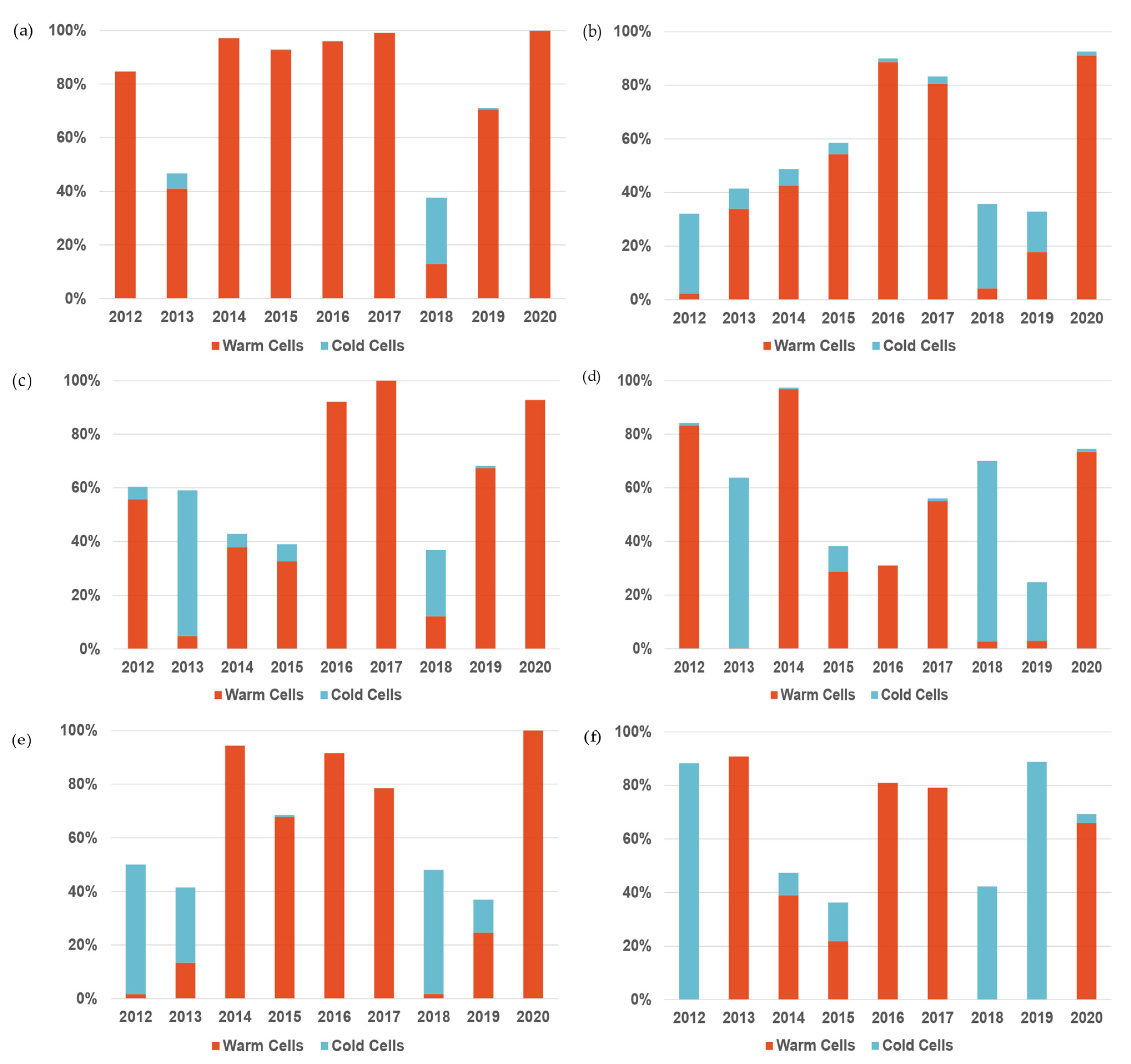
To comprehensively account for the distinct oceanographic dynamics in the CCUS, we analyzed the SST changes within the defined regions. By computing the percentages of warming and cooling cells within each of the delineated regions, a refined evaluation of localized climatic trends was achieved, which might have been obscured in an overarching assessment of the entire study area. Through this approach, we aimed to uncover region-specific deviations that could otherwise be overshadowed. This meticulous regional analysis enhanced our grasp of the intricate interactions characterizing the CCUS oceanography. Notably, these regions exhibited not only unique SST patterns but also distinctive oceanic attributes. For example, the presence of the Coastal Countercurrent along the SW Iberian coast imparted specific characteristics to the nearshore and offshore zones. The results are shown in Figure 8.

Each graph in Figure 8 shows a higher concentration of warm cell percentage in the offshore region compared to the corresponding nearshore region, where there is a presence of both warming and cooling cells. The Canary offshore region shows the highest percentage of warming cells, with percentages reaching nearly 100%. Comparison between nearshore and offshore regions indicates that SST in the offshore region is higher than SST in the corresponding adjacent nearshore region. In terms of the rates of SST change since the end of the 1982–2012 baseline period, the Canary offshore region has shown a significantly higher percentage of warming areas compared to its adjacent nearshore region for each year from 2012 through 2020. The same pattern is also found off the coast of West Iberia. The nearshore region off the southwestern coast of Iberia exhibits a notable prevalence of cooling cells. Of particular interest is the observed decoupling in SST between this region and the broader West Iberia nearshore area, as depicted in Figure 8d. This decoupling phenomenon is especially prominent in the years 2012 and 2013. The divergence between the SST patterns in Figure 8d,f can be attributed to variations in the intensity of upwelling processes occurring near Cape São Vicente, as described by Relvas and Barton [16]. These differences in SST patterns are therefore linked to variations in the upwelling dynamics near Cape São Vicente compared to those along the remainder of the West Iberia nearshore region.

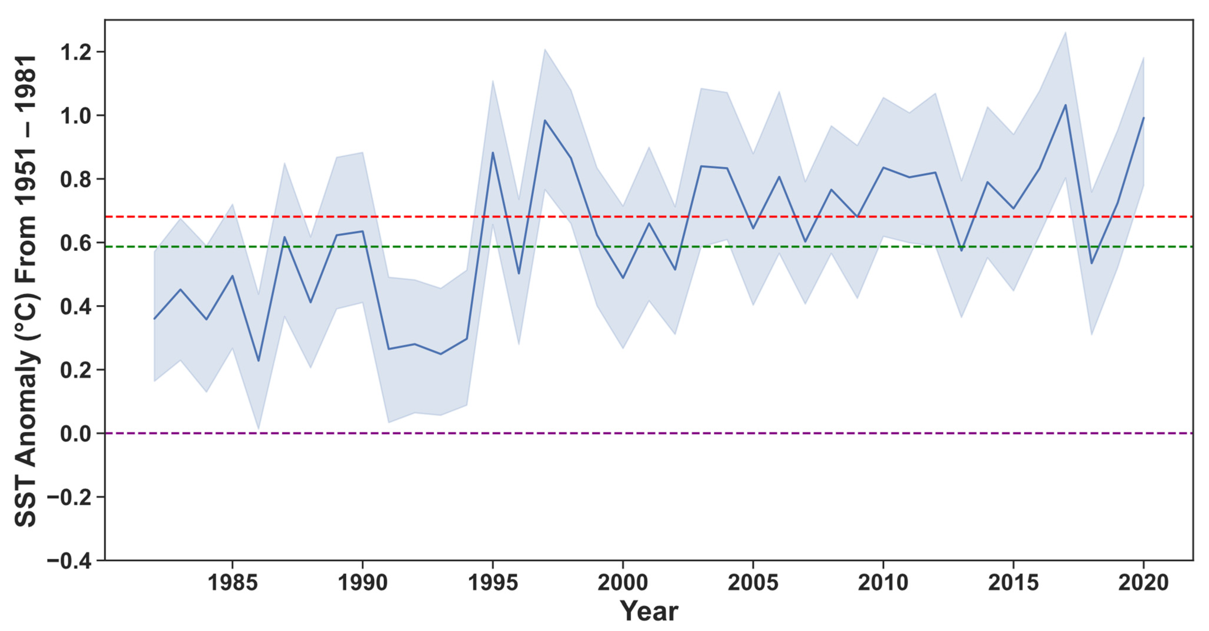
To assess how each year deviates from the baseline periods over the entire region, SST anomaly time series graphs were computed. These were conducted for each of the three baselines (1951–1981, 1982–2012, and 1990–2020). Each yearly SST from 1982 to 2020 is shown, using the 1951–1981 baseline period as a reference, with the remaining two baselines shown as anomalies in relation to the 1951–1981 baseline. 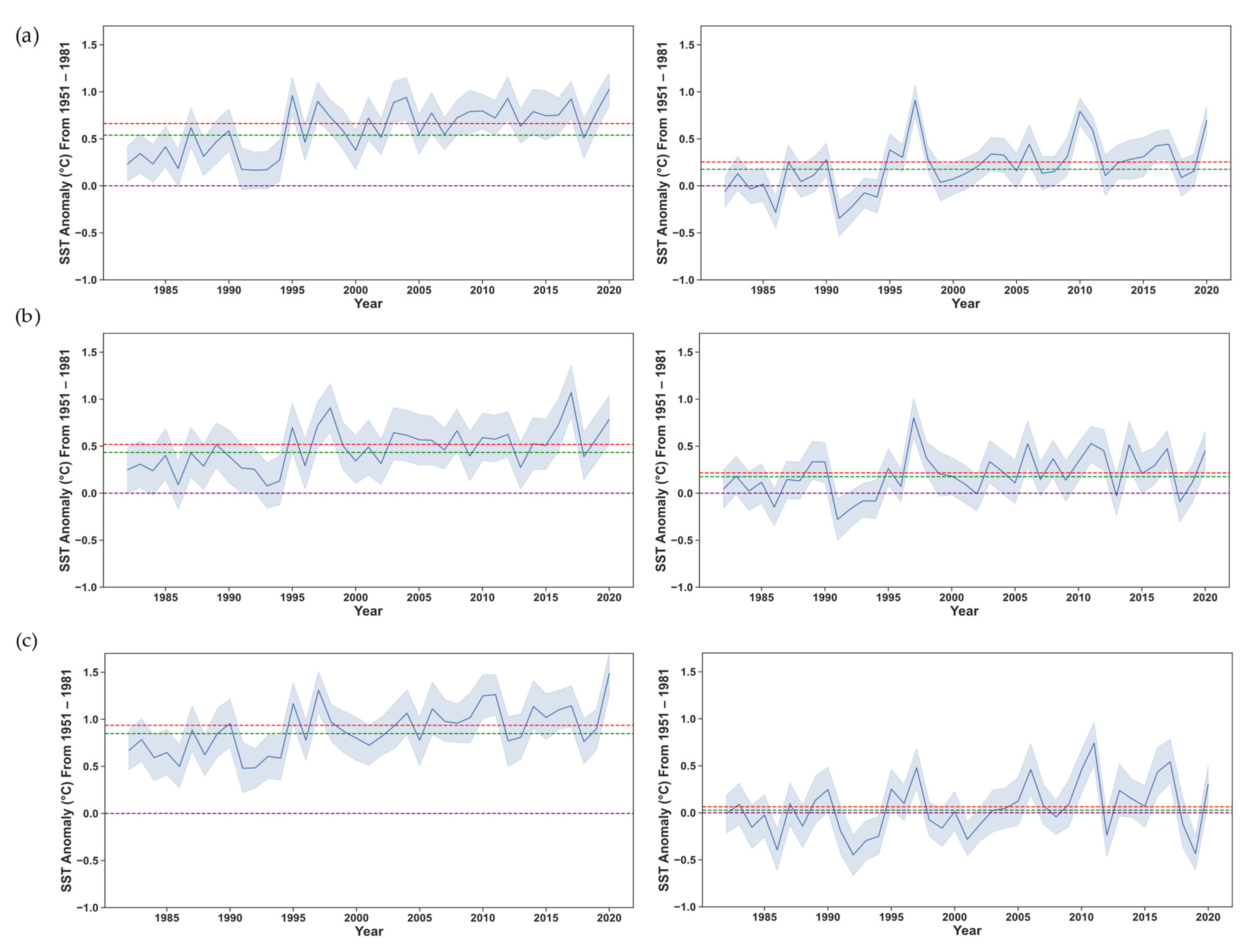The SST anomaly time series graph for the entire study area is shown in Figure 9. The same algorithm was applied to the three nearshore regions and the corresponding three offshore regions, resulting in six yearly time series graphs. Figure 10 shows the yearly time series graphs for each region using the 1951–1981 baseline period as a reference.

Based on the results of Figure 9, it is possible to depict a marked increase in SST when comparing the 1951–1981 baseline to the 1982–2012 baseline where the 30-year climatological normal SST increases by 0.59 °C. The 1991–2020 baseline continues to increase, but at a much slower rate with an increase of 0.1 °C from the 1982–2012 baseline to the 1991–2020 baseline. The yearly SST values are markedly higher than the 1951–1981 baseline but vary between the 1982–2012 and 1991–2020 baselines. This reveals how climate change has impacted SST and how the SST baselines have increased dramatically after the 1951–1981 climatological period. However, this has decelerated from the 1982–2012 baseline to the 1991–2020 baseline. The sudden increase in SST from the 1951–1981 baseline to the 1982–2012 baseline is much more evident in the offshore regions compared to their corresponding nearshore regions (Figure 10). For example, the differences in mean SST between the 1951–1981 baseline period and the 1982–2012 baseline period for the Canary offshore region is 0.54 °C, while for the corresponding nearshore region it is 0.17 °C. The same pattern holds for West Iberia, with an SST anomaly between the two baselines of 0.43 °C for the offshore region and 0.17 °C for the nearshore region, as well as SW Iberia, with an SST anomaly of 0.84 °C for the offshore region and 0.24 °C for the nearshore region.

To quantify the differences between the three baseline periods and to assess how SST has changed over the long term, SST was averaged over each different baseline for the entire study area as well as each nearshore and corresponding offshore region.

Table 2. SST averages for the three different baselines over the entire regional domain and nearshore and offshore regions.

	SST (°C)
	1951–1981	1982–2012	1991–2020
Full study area	17.70	18.29	18.38
Canary Offshore	19.59	20.13	20.25
Canary Nearshore	19.14	19.31	19.39
West Iberia Offshore	16.66	17.09	17.18
West Iberia Nearshore	16.22	16.39	16.43
SW Iberia Offshore	18.42	19.26	19.35
SW Iberia Nearshore	18.23	18.47	18.51

summarizes how SST has shifted in the long term both temporally and spatially, demonstrating a marked overall increase of 0.59 °C between the 1951–1981 baseline (17.70 °C) and the 1982–2012 baseline (18.29 °C). The 1991–2020 baseline continues to increase but at a lower rate, with a difference of 0.09 °C compared to the 1982–2012 baseline. The increase in SST between the baselines is consistently higher in the offshore regions compared to their corresponding nearshore regions. The rate of SST change decelerates for the nearshore regions when comparing the latter two baseline periods but does not yet begin to decrease, as evident in the anomaly maps in Figure 6. Figure 6 represents immediate changes in SST that occur directly after the 1982–2012 baseline period, whereas Table 2 shows the long-term trends for the different baseline periods considered. Thus, the cooling trend in the nearshore regions is evident when looking at SST in the short term after the 1982–2012 baseline, but is not yet evident when evaluating SST in the long term.

The nearshore and offshore time series graphs (Figure 10) show less variability between the three baselines for the nearshore regions compared to their corresponding offshore regions. The anomaly time series for the offshore regions show a more consistent increase in SST for each year and each baseline, whereas the nearshore regions show more variability on a year-to-year basis but less variability between the 30-year climatological baselines periods.

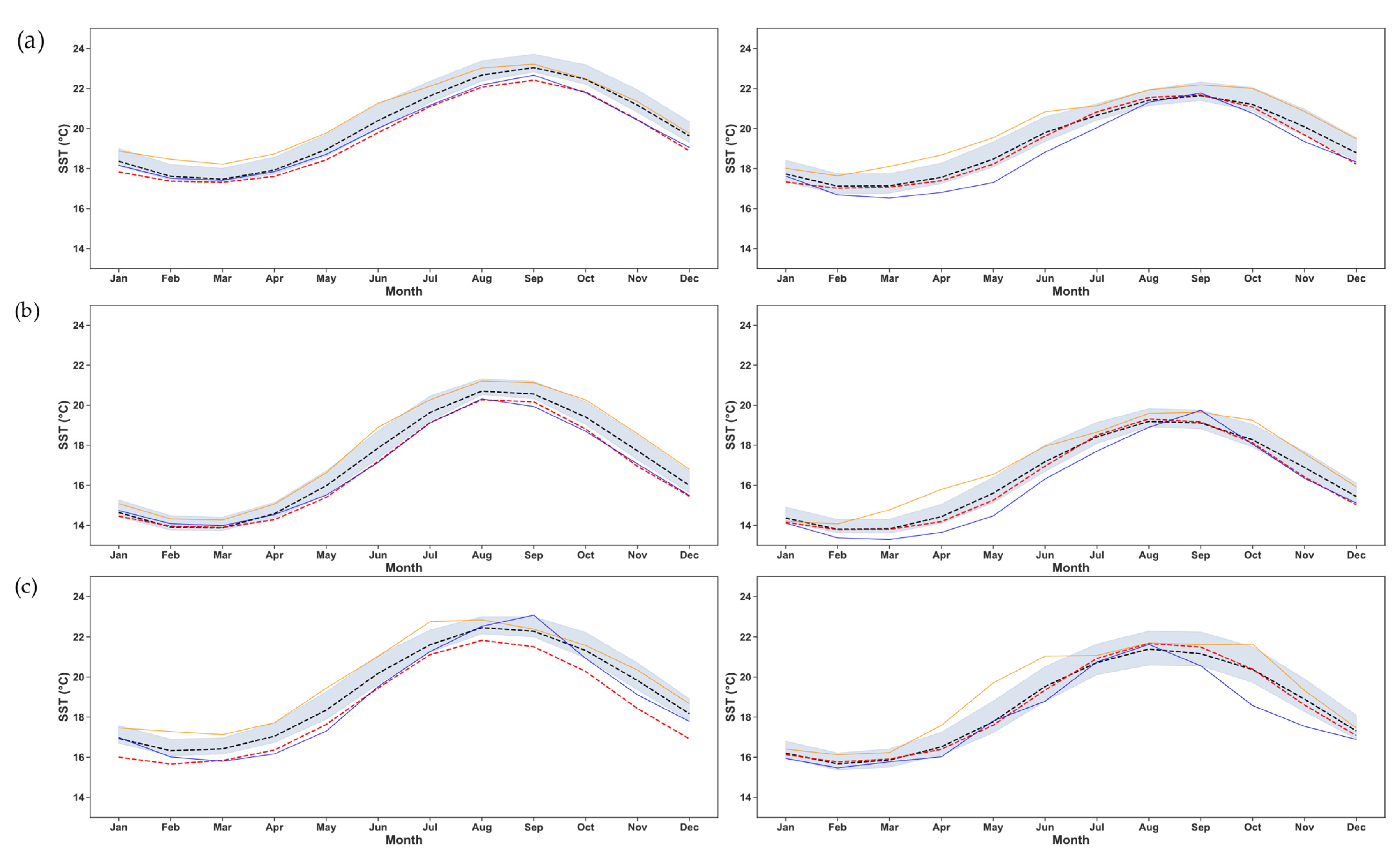
In terms of the interannual variability in SST at each of the three nearshore regions compared to the three offshore regions, monthly mean time series were also computed for each region and are presented in Figure 11. The results corroborate the findings above, with offshore regions all showing consistent increases in SST, whereas the nearshore regions show lower SST values and much more variability between the years. The region with the most variability is South Iberia (Figure 11c), where it can also be noted that in the offshore region the year with the lowest SST highlighted in blue (1991) has significantly higher SST values during the summer months but considerably lower SST values during the spring and winter months. The high interannual variability in both the nearshore and offshore regions of South Iberia can be attributed to the complexity of the water circulation, where the interaction between the Coastal Countercurrent and adjacent oceanic currents plays a major role.

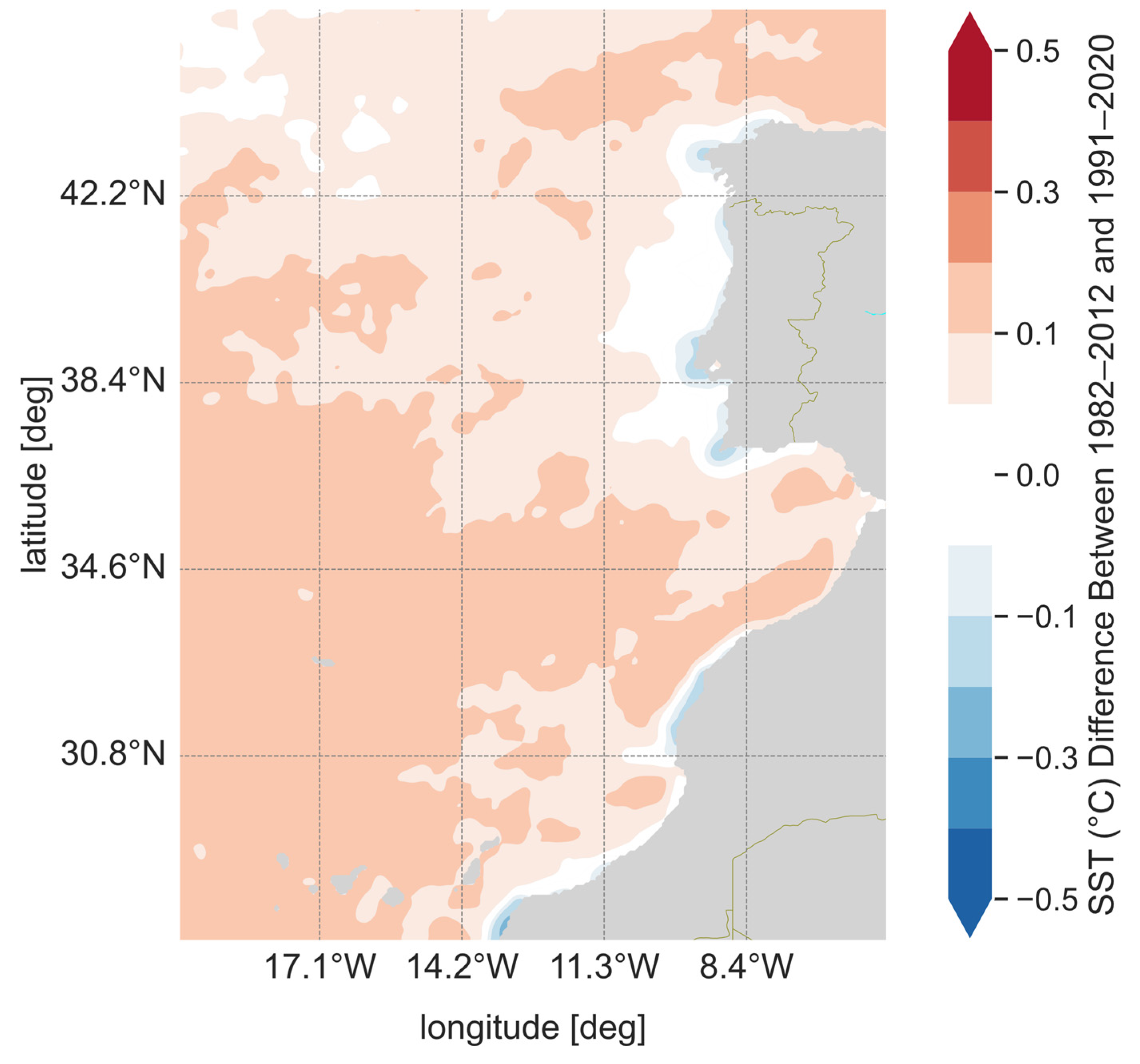
Since the new 30-year climate normal period from 2020 onward will now be 1991–2020, SST from the new satellite product during this period was also assessed and compared to the baseline period used for this study (1982–2012). The anomaly between these two baseline periods is shown in Figure 12, which shows a marked increase in SST offshore from the 1982–2012 baseline to the 1991–2020 baseline. This observation reinforces the long-term increasing SST trend that has been consistently noted in the offshore regions. Conversely, closer to shore, the SST anomaly between the two baselines has predominantly shown no significant change, with certain specific regions such as Cape São Vicente registering a decrease in SST between 0.1 °C and 0.2 °C. These findings underscore the significant influence of upwelling processes in coastal areas. The declining SST in this region may signify an intensification of upwelling dynamics as colder, deeper waters are transported to the surface.

4. Conclusions

This comprehensive study of the CCUS, with its particular focus on SST changes, underscores the intricate interplay between oceanographic phenomena and their broader ecological and socio-economic impacts. The CCUS, characterized by significant upwelling events off the west coast of the Iberian Peninsula and along the northwest coast of Africa, plays a crucial role in sustaining high marine productivity and biodiversity. This system, vital for an array of marine species including economically important fish stocks, is sensitive to alterations induced by climate change, particularly to changes in SST.

Our analysis, leveraging high-resolution satellite data over the last 40 years, successfully characterizes and quantifies SST changes in the CCUS region. Acknowledging the limitations of the remotely sensed data, our approach validates these findings with in situ measurements, ensuring a comprehensive and accurate representation of SST changes. The ODYSSEA Level 4 Sea Surface Temperature Reprocessed dataset, known for its high resolution and quality, underpins our analysis, mitigating common issues associated with satellite data. This climatological assessment, comparing current SST trends with a standardized reference period (1951–1981), reveals a non-uniform increase in SST, which is higher in offshore waters compared to nearshore waters where upwelling is more influential. The study highlights the spatial and seasonal variability in SST, with nearshore areas experiencing a slower rate of warming due to the cooling effects of upwelling, especially evident during the summer months.

In regional terms, SST in the CCUS is shown to increase when comparing the two baseline periods and has been rising since the baseline period of 1982–2012. The rates of SST vary both spatially and seasonally. SST is rising at a much slower rate at the coast. In summer, the offshore and nearshore differences are enhanced, especially off the west and southern coast of Portugal when upwelling occurs. Off the coast of West Africa, the differences in SST between nearshore and offshore waters remain almost the same throughout the year. Previous studies analyzing SST in the CCUS have drawn similar conclusions about the slower rate of SST warming nearshore compared to offshore [21].

The implications of our findings are far-reaching. Changes in SST and upwelling patterns directly affect the quantity and distribution of marine species, impacting local fisheries and the socio-economic fabric of coastal communities. SST changes serve as indicators of broader ecological shifts, influencing the breeding, spawning, and migration patterns of marine species and thus altering the ecological balance of the region.

Looking ahead, this study identifies the need for further investigation into the specific mechanisms of upwelling in the CCUS and their differential effects on SST. A more in-depth comparative analysis across seasons and over extended periods will enhance our understanding of upwelling intensity and frequency on SST variability. Historical data and advanced climate models simulating future SST trends will augment our understanding and predict the impacts of climate change in the CCUS region.

Future studies should also integrate SST data with biological data on pelagic species to establish correlations between SST change and reproductive parameters. This can be achieved through the development of ecological and population models to simulate different scenarios of SST change and assess its impacts on the life cycle and reproductive strategies of pelagic species. Historical data on fish catch can also be correlated with past SST trends to determine how these species have adapted to previous climate variations. In the southern region of the CCUS, where data on the relationship between environment and recruitment variability are limited, remotely sensed products characterizing coastal winds as well as ocean color products determining nutrient dynamics should be utilized. It is imperative to further validate these data sources with in situ measurements in the region. This comprehensive analysis can be used to predict pelagic species’ response to SST change in the long term.

In an era of evolving climate patterns, understanding the complex dynamics of our oceans is imperative. This study not only enriches our knowledge of the CCUS but also sets the stage for future investigations into changing climatological patterns in coastal regions. As we anticipate and adapt to the impacts of climate change, incorporating finer-resolution remotely sensed data will be crucial in future climatological studies, especially for investigating the nuanced upwelling features of nearshore regions. Our continued efforts in this domain are essential for safeguarding these vital oceanic ecosystems and the communities that depend on them.