A Cloud Detection Algorithm Based on FY-4A/GIIRS Infrared Hyperspectral Observations

Abstract

Cloud detection is an essential preprocessing step when using satellite-borne infrared hyperspectral sounders for data assimilation and atmospheric retrieval. In this study, we propose a cloud detection algorithm based solely on the sensitivity and detection characteristics of the FY-4A Geostationary Interferometric Infrared Sounder (GIIRS), rather than relying on other instruments. The algorithm consists of four steps: (1) combining observed radiation and clear radiance data simulated by the Community Radiative Transfer Model (CRTM) to identify clear fields of view (FOVs); (2) determining the number of clouds within adjacent 2 × 2 FOVs via a principal component analysis of observed radiation; (3) identifying whether there are large observed radiance differences between adjacent 2 × 2 FOVs to determine the mixture of clear skies and clouds; and (4) assigning adjacent 2 × 2 FOVs as a cloud cluster following the three steps above to select an appropriate classification threshold. The classification results within each cloud detection cluster were divided into the following categories: clear, partly cloudy, or overcast. The proposed cloud detection algorithm was tested using one month of GIIRS observations from May 2022 in this study. The cloud detection and classification results were compared with the FY-4A Advanced Geostationary Radiation Imager (AGRI)’s operational cloud mask products to evaluate their performance. The results showed that the algorithm’s performance is significantly influenced by the surface type. Among all-day observations, the highest recognition performance was achieved over the ocean, followed by land surfaces, with the lowest performance observed over deep inland water. The proposed algorithm demonstrated better clear sky recognition during the nighttime for ocean and land surfaces, while its performance was higher for partly cloudy and overcast conditions during the day. However, for inland water surfaces, the algorithm consistently exhibited a lower cloud recognition performance during both the day and night. Moreover, in contrast to the GIIRS’s Level 2 cloud mask (CLM) product, the proposed algorithm was able to identify partly cloudy conditions. The algorithm’s classification results departed slightly from those of the AGRI’s cloud mask product in areas with clear sky/cloud boundaries and minimal convective cloud coverage; this was attributed to the misclassification of clear sky as partly cloudy under a low-resolution situation. AGRI’s CLM products, temporally and spatially collocated to the GIIRS FOV, served as the reference value. The proportion of FOVs consistently classified as partly cloudy to the total number of partly cloudy FOVs was 40.6%. In comparison with the GIIRS’s L2 product, the proposed algorithm improved the identification performance by around 10%.

1. Introduction

The use of satellite information has improved numerical weather prediction results and increased forecasts’ reliability [1,2]. As a result, the contribution of satellite data to numerical forecasting systems has steadily grown. Statistics from the European Centre for Medium-Range Weather Forecasts (ECMWF) show that 91.41% of data input to the assimilation system come from satellite observations [3]. Having analyzed and assessed the impact of the initial decade of use of the TIROS Operational Vertical Sounder (TOVS) on weather forecasting, the World Meteorological Organization (WMO) concluded that significant improvements in weather forecasting capabilities could exclusively improve the precision of global atmospheric vertical temperature and humidity profiles to equal that of radio soundings [4]. Among the various types of satellite remote sensing data, high-spectral infrared data have emerged as crucial for reducing forecast errors and enhancing assimilation effects in all satellite observations [5].

Spaceborne infrared hyperspectral sounders, which boast a high detection capability, a high spectral resolution, and spectral coverage of CO₂ and H₂O absorption bands, predominantly provide information on atmospheric temperature and humidity [6]. Their high spectral resolution provides a high vertical resolution, allowing for fine-scale detection of meteorological elements (especially temperature and humidity) throughout the atmospheric troposphere. They are the most important satellite data source, reducing forecast errors and improving assimilation effectiveness [5]. In particular, an infrared hyperspectral sounder mounted on a geostationary mereological satellite platform facilitates continuous observations of the covered area with a high temporal resolution. As small- and medium-scale weather systems evolve relatively quickly, these high temporal resolution instruments are important for detecting high-impact weather events that are strongly associated with atmospheric thermodynamic instability, as well as convective systems that develop over a short period of time [7]. Therefore, observations from geostationary hyperspectral infrared sounders are crucial for weather monitoring and numerical prediction models [8].

FY-4A is a Chinese second-generation geostationary meteorological satellite, positioned at 104.7°E over the equator. It has a more than 20-fold increased observation efficiency and can perform 24 h Earth observations from high altitudes [9]. The Geostationary Interferometric Infrared Sounder (GIIRS) is the world’s first precision infrared hyperspectral instrument specifically designed to measure the vertical structure of the atmosphere in geostationary orbit via infrared interferometric spectroscopy. The GIIRS covers the mid-wave infrared (1650–2250 cm⁻¹) and longwave infrared (700–1130 cm⁻¹) bands at a spectral resolution of 0.625 cm⁻¹. It comprises 1650 observation channels, with 689 channels in the longwave and 961 channels in the mid-wave band.

Atmospheric clouds exhibit a high forecast sensitivity [10], and their role in the radiative balance of the Earth’s atmospheric system is determined by their optical properties [11]. Clouds consist of water droplets and ice crystals, both of which strongly absorb infrared radiation, and can be approximated as black bodies [12]. If clouds are present in the field of view, the infrared radiation emitted by the atmosphere below clouds cannot be distinguished from the radiance from clouds [13]. Cloud detection, which determines if there is any cloud cover in each satellite instrument’s instantaneous field of view, is a fundamental and essential step for atmospheric parameter retrieval and cloud microphysical property retrieval. Cloud detection also plays a critical role in clear-sky and cloud-area satellite data assimilation. Therefore, in practical applications of infrared data, it is often necessary to first eliminate cloud-contaminated scenes [14].

The common methods for cloud detection can be grouped into four types: finding ‘clear FOVs’ [15]; ‘clear channels’ [16]; ‘cloud clearing’ [17]; and ‘cloud product matching between different instruments’ [18]. The ‘clear FOV’ approach aims to find completely cloud-free fields of view (FOVs) by excluding observations from all channels within cloudy FOVs. For example, Wang et al. selected optimal channels for the FY-4A GIIRS’s mid-wave infrared band and used the minimum residual method to calculate the effective cloud cover for cloud classification [19]. The ‘clear channel’ method does not completely eliminate clouds from the satellite’s FOV. Instead, it assigns cloud-free channel heights to different channels based on their varying sensitivities to clouds. This method, proposed by McNally et al. (2003), is employed by the ECMWF for cloud detection using an Atmospheric Infrared Sounder (AIRS) and an Infrared Atmospheric Sounding Interferometer (IASI) [20]. The ‘cloud clearing’ method combines moderate-resolution spectroradiometer imaging data with AIRS FOV radiance data equivalent to a clear sky and was proposed by Li et al. Finally, as an example of cloud product matching, Guan et al. (2007). performed spatial and temporal matching of high-resolution Moderate-resolution Imaging Spectroradiometer (MODIS) imager cloud detection products to AIRS’s FOVs for successful cloud detection [21]. In addition, based on the clear channel method, Li et al. added Advanced Himawari Imager (AHI) cloud mask products to select clear sky areas and remove high-level clouds. This two-step cloud detection method serves as a complementary method for clear sky areas [22].

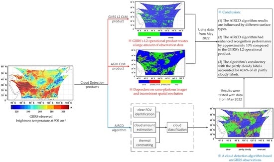
These cloud detection algorithms are mainly used on polar-orbiting satellites, which have limitations in capturing rapidly developing weather systems due to their poor temporal resolution. In contrast, geostationary satellites offer high spectral and temporal resolutions. They can continuously monitor rapid and intense changes in water vapor levels and temperatures during severe weather events when compared to infrared hyperspectral detection instruments on polar-orbiting satellites. At present, the GIIRS Level 2 (L2) operational cloud mask (CLM) product relies on the Advanced Geostationary Radiation Imager (AGRI) mounted on the same satellite [23]. The high-spatial-resolution imager cloud mask product is spatially and temporally matched to the low-spatial-resolution GIIRS’s FOV. Cloud detection in the GIIRS’s FOV is based on the proportion of AGRI clear/cloud pixels within it. This method only processes clear-sky FOVs and eliminates scenes contaminated by clouds, which wastes a large amount of observation data. Thus, it is desirable to develop a cloud detection algorithm that is based solely on GIIRS observations and does not rely on other instruments.

A cloud detection algorithm based solely on FY-4A GIIRS observations (advanced infrared hyperspectral cloud detection, hereafter referred to as AIRCD) is proposed in this paper according to the basic principles of cloud detection proposed by the Cross-track Infrared and Microwave Sounding Suite Environmental Data Records (CrIMSS EDR) algorithm [24]. The algorithm employs the following four steps to extract cloud information and determine cloud coverage in the GIIRS’s FOV: (1) clear FOV identification, (2) cloud amount estimation, (3) thermal contrasting, and (4) cloud classification.

2. Data and Radiative Transfer Model

2.1. Data

The data used in this research include FY-4A GIIRS observations, AGRI products, and ERA5 reanalysis data; the details are as follows.

The GIIRS observes China and its surrounding areas (3–55°N, 60–137°E) every 2 h. The FY-4A GIIRS’s coverage extends from north to south and comprises seven latitudinal scan lines, each comprising 59 fields of regard (FORs). The FOVs for GIIRS’s observation mode are arranged in a 32 × 4 array, where each FOV corresponds to a specific detector and provides a spatial horizontal resolution of approximately 16 km. GIIRS Level 1 (L1) radiance observations with a spatial resolution of 16 km and L2 CLM products at 1200–1340 UTC on 13 May 2022 were used. GIIRS L1 and L2 datasets were obtained from the Chinese National Satellite Meteorological Center (http://satellite.nsmc.org.cn, accessed on 8 October 2023).

The full-disk cloud mask products derived from the FY-4A AGRI with a 4 km resolution at 1300–1315 UTC on 13 May 2022 were used as reference values to examine the cloud detection results. The AGRI is the primary optical payload onboard FY-4A, providing extensive coverage of Earth’s atmosphere every 15 min. The AGRI’s operational CLM products with a high spatial resolution and reliability are generated in real time. The CLM values were classified as 0 = cloud; 1 = probably cloud; 2 = probably clear; and 3 = clear. The AGRI L2 data were also sourced from http://satellite.nsmc.org.cn, accessed on 8 October 2023.

The atmospheric state parameters from ERA5 were used as inputs in the fast radiative transfer model to simulate satellite measurements. The ERA5 reanalysis dataset has a horizontal resolution of 0.25 × 0.25°, a temporal resolution of 1 h, and is vertically divided into 37 levels extending from the surface to 0.01 hPa. Since the ERA5 data and GIIRS observations have different spatial and temporal resolutions, the ERA5 data needed to be spatially interpolated to each GIIRS’s FOV before simulating the brightness temperature via the radiative transfer model. The ERA5 values at the nearest four grid points were selected for distance-weighted averaging. The maximum time matching difference is 1 h. The ERA5 datasets were obtained from the Meteorological Archival and Retrieval System (MARS, https://cds.climate.copernicus.eu, accessed on 8 October 2023).

2.2. Radiative Transfer Model

The Community Radiative Transfer Model (CRTM) was used to simulate satellite observations. Developed by the Joint Center for Satellite Data Assimilation (JCSDA) in the USA, the CRTM was designed to simulate satellite observations in the ultraviolet, visible, infrared, and microwave bands. It comprises four modules: the forward, tangent, adjoint, and K-matrix modules [25]. During forward module calculations, the CRTM simulates the radiation received in the observation direction of the satellite instrument. The input ERA5 atmospheric state parameters for the CRTM include atmospheric temperature profiles, specific humidity profiles, ozone mixing ratio profiles, and surface parameters such as wind speed at 10 m, temperature at 2 m, surface pressure, and surface temperature. Additionally, the satellite’s scan angles, zenith angles, and azimuth angles need to be input. These are then combined with the spectral response function of the satellite instrument’s observation channel to simulate the brightness temperatures.

3. Cloud Detection Algorithm Based on GIIRS Observations

As mentioned in Section 2.1, for the cloud detection algorithm, adjacent 2 × 2 FOVs were selected as samples according to the arrangement of the FY-4A GIIRS’s scanning detectors. Each FOR contains 16 × 2 cloud detection clusters, as shown by the black circles in Figure 1.

The physical basis of cloud detection lies in the fact that when detecting the wavelength in a specific infrared channel, the detected thermal energy of an object is mainly related to its own temperature [26]. What sets clouds apart from other underlying surfaces is that they have high reflectance and low brightness temperatures. During cloud detection tasks, brightness temperature differences can be used to distinguish between clouds and a clear sky. The principle is that a single scattering by clouds results in changes in spectral information. Additionally, there is a nonlinear variation in the Planck function during this process; in other words, it expresses the temperature difference between clouds and different surface types. The absorption and emission of other factors are not considered in this process. Changes in spectral information are often influenced by the microphysical properties of the clouds. Therefore, infrared brightness temperature differences can distinguish between clouds and clear skies [27].

The most significant infrared absorption bands for atmospheric CO₂ are the 4.3 μm and 15 μm bands. When clouds are present in the FOV, the attenuation of brightness temperature is significantly greater in the shortwave infrared channel than in the longwave infrared channel; this discrepancy arises from the strong scattering effect of ice particles and can be effectively used for cloud detection. Therefore, we based the AIRCD algorithm on the dual gas absorption bands of CO₂ in the GIIRS, which are the longwave infrared band at 709.5–746.0 cm⁻¹ and the shortwave infrared band at 2190–2250 cm⁻¹.

A flow chart of the cloud detection algorithm is shown in Figure 2. The process is divided into four steps: clear FOV identification, cloud amount estimation, thermal contrasting, and cloud classification. The classification results within each cloud detection cluster are divided into the following categories: clear, partly cloudy, or overcast.

3.1. Clear FOV Identification

We observed no significant differences in the overall observed radiance in each FOV when the cloud detection cluster was in either overcast or clear sky conditions (i.e., the scene was relatively homogeneous) [28]. Therefore, to determine whether a cloud detection cluster consisting of 2 × 2 FOVs was clear, the number of clear FOVs within the cluster was first calculated. The clear radiance of each FOV was simulated using the CRTM. The root-mean-square error of radiances (${\mathrm{d}\mathrm{y}}_{\mathrm{j}}$) between the observed and simulated clear radiations for all channels in the longwave infrared band of 709.5–746.0 cm⁻¹ was calculated as follows:

$${\mathrm{d}\mathrm{y}}_{\mathrm{j}}=\sqrt{\frac{{\displaystyle \sum _{\mathrm{i}=1}^{\mathrm{n}\mathrm{c}\mathrm{h}\mathrm{a}\mathrm{n}}}{({\mathrm{R}}_{\mathrm{i}\mathrm{j}}-{\mathrm{R}}_{\mathrm{i}\mathrm{j}}^{\mathrm{c}\mathrm{l}\mathrm{r}})}^2}{\mathrm{n}\mathrm{c}\mathrm{h}\mathrm{a}\mathrm{n}}}$$

(1)

where ${\mathrm{R}}_{\mathrm{i}\mathrm{j}}$ and ${\mathrm{R}}_{\mathrm{i}\mathrm{j}}^{\mathrm{c}\mathrm{l}\mathrm{r}}$ denote the radiances in FOV $\mathrm{j}$ and channel $\mathrm{i}$ for the observed and simulated clear FOVs, respectively, and ‘$\mathrm{n}\mathrm{c}\mathrm{h}\mathrm{a}\mathrm{n}$’ is the 59 channels in the 709.5–746.0 cm⁻¹ band.

Ideally, if the FOV is clear, the radiance observed by the satellite should be the same as the simulated clear radiance. However, the difference between the observed and simulated radiance can be affected by instrument noise and the simulation error of the radiative transfer model. Thus, the conditions used to determine a clear FOV were as follows:

$${\mathsf{\sigma }}_{\mathrm{j}}=\sqrt{\frac{{\displaystyle \sum _{\mathrm{i}=1}^{\mathrm{n}\mathrm{c}\mathrm{h}\mathrm{a}\mathrm{n}}}{\mathrm{N}\mathrm{e}∆\mathrm{R}(\mathrm{i},\mathrm{j})}^2}{\mathrm{n}\mathrm{c}\mathrm{h}\mathrm{a}\mathrm{n}}}$$

(2)

where $\mathrm{N}\mathrm{e}\Delta \mathrm{R}(\mathrm{i},\mathrm{j})$ denotes the noise-equivalent radiance in FOV $\mathrm{j}$ and channel $\mathrm{i}$ and comes from the GIIRS Level 1 dataset. ${\mathsf{\sigma }}_{\mathrm{j}}$ was obtained by averaging the $\mathrm{N}\mathrm{e}\Delta \mathrm{R}$ of all channels within the 709.5–746.0 cm⁻¹ band for each FOV_j. If ${\mathrm{d}\mathrm{y}}_{\mathrm{j}}<10\sqrt{2}{\mathsf{\sigma }}_{\mathrm{j}}$, the FOV is clear; otherwise, it is overcast [24]. The number of clear FOVs within the cloud detection cluster is denoted as ${\mathrm{N}}_{\mathrm{c}\mathrm{l}\mathrm{r}}$ in Equations (1) and (2).

3.2. Cloud Amount Estimation

In this step, a principal component analysis is used to determine the number of cloudy FOVs within a cloud detection cluster and to initially distinguish between clear, overcast, and partly cloudy conditions. For the four FOVs within the cloud detection cluster, the GIIRS-observed radiance of all channels in the longwave infrared band ranges from 709.5 cm⁻¹ to 746.0 cm⁻¹, forming a 4 × 59 matrix. A principal component analysis was applied to this matrix to obtain the four orthogonal principal components and their corresponding eigenvalues. Susskind et al., (2003) indicated that principal components with larger eigenvalues are informative, whereas others are typically associated with the observed noise [29]. The cloud amount is approximately equal to the number of significant principal components within the cloud detection cluster that corresponds to the cloud features.

First, we calculated the residual standard deviation (RSD) of the last few eigenvalues and estimated the observed noise, $\mathsf{\sigma }$:

$${\mathrm{R}\mathrm{S}\mathrm{D}}_{\mathrm{n}}={\left[\frac{1}{\mathrm{n}\mathrm{c}\mathrm{h}\mathrm{a}\mathrm{n}\times (\mathrm{n}\mathrm{f}\mathrm{o}\mathrm{v}-\mathrm{n})}{\sum }_{\mathrm{j}=\mathrm{n}+1}^{\mathrm{n}\mathrm{f}\mathrm{o}\mathrm{v}}{\mathsf{\lambda }}_{\mathrm{j}}\right]}^{1/2}$$

(3)

$$\mathsf{\sigma }=\frac{1}{1.5\times \mathrm{n}\mathrm{f}\mathrm{o}\mathrm{v}}{\sum }_{\mathrm{i}=1}^{\mathrm{n}\mathrm{c}\mathrm{h}\mathrm{a}\mathrm{n}}{\sum }_{\mathrm{j}=1}^{\mathrm{n}\mathrm{f}\mathrm{o}\mathrm{v}}{\mathrm{N}\mathrm{e}\Delta \mathrm{R}(\mathrm{i},\mathrm{j})}^2$$

(4)

where ${\mathsf{\lambda }}_{\mathrm{j}}$ is the eigenvalue and $\mathrm{n}\mathrm{f}\mathrm{o}\mathrm{v}=4$, $\mathrm{n}\le \mathrm{n}\mathrm{f}\mathrm{o}\mathrm{v}$, where n takes values from one in sequence. When ${\mathrm{R}\mathrm{S}\mathrm{D}}_{\mathrm{n}}\le \mathsf{\sigma }$, the number of significant principal components is $\mathrm{n},$ and the cloud amount ${\mathrm{N}}_{\mathrm{c}\mathrm{f}1}=\mathrm{n}-1$.

Second, the chi-square, ${{\chi }_{\mathrm{n}}}^2,$ was calculated in turn from the observed radiance and radiance for the first n principal component reconstructions, ${\widehat{\mathrm{R}}}_{\mathrm{i}\mathrm{j}}\left(\mathrm{n}\right)$:

$${{\chi }_{\mathrm{n}}}^2={\sum }_{\mathrm{i}=1}^{\mathrm{C}\mathrm{h}\mathrm{a}\mathrm{n}}{\sum }_{\mathrm{j}=1}^{\mathrm{F}\mathrm{O}\mathrm{V}}\frac{{\left[{\mathrm{R}}_{\mathrm{i}\mathrm{j}}-{\widehat{\mathrm{R}}}_{\mathrm{i}\mathrm{j}}\left(\mathrm{n}\right)\right]}^2}{{\mathrm{N}\mathrm{e}\Delta \mathrm{R}(\mathrm{i},\mathrm{j})}^2}$$

(5)

The reconstructed radiance, ${\widehat{\mathrm{R}}}_{\mathrm{i}\mathrm{j}}\left(\mathrm{n}\right),$ was computed using the mat function with four principal components and their corresponding eigenvalues. As the number of principal components, n, used for radiance reconstruction increases, the minimum n that satisfies ${{\chi }_{\mathrm{n}}}^2<\left(\mathrm{n}\mathrm{f}\mathrm{o}\mathrm{v}-\mathrm{n}\right)\times \left(\mathrm{n}\mathrm{c}\mathrm{h}\mathrm{a}\mathrm{n}-\mathrm{n}\right)$ corresponds to the significant principal components related to the cloud. At this point, the reconstructed radiance, ${\widehat{\mathrm{R}}}_{\mathrm{i}\mathrm{j}}\left(\mathrm{n}\right),$ was already approximately representative of the original radiance, and the cloud amount ${\mathrm{N}}_{\mathrm{c}\mathrm{f}2}=\mathrm{n}-1$. After comparing the values of ${\mathrm{N}}_{\mathrm{c}\mathrm{f}1}$ and ${\mathrm{N}}_{\mathrm{c}\mathrm{f}2}$ obtained in the above two steps, we used the larger value as the cloud amount, ${\mathrm{N}}_{\mathrm{c}\mathrm{f}}$, of the cloud detection cluster.

3.3. Thermal Contrasting

The difference in observed radiance between FOVs is more significant when partial cloud contamination exists within the cloud detection cluster. In contrast, the observed radiance between FOVs is similar under overcast or clear sky conditions. Thus, to further distinguish partly cloudy conditions, a thermal contrast test is required.

The average observed radiances for the 709.5–746.0 cm⁻¹ and 2190–2250 cm⁻¹ channels of the four FOVs within the cloud detection cluster were sorted in descending order. The FOV with the highest average radiance was labeled as the ‘warmest’ FOV, whereas that with the lowest average radiance was labeled as the ‘coldest’ FOV. The absolute difference in observations between the ‘warmest’ and ‘coldest’ FOVs was then calculated and compared with the GIIRS channel noise.

$${\mathrm{T}\mathrm{c}\mathrm{t}\mathrm{e}\mathrm{s}\mathrm{t}1}_{\mathrm{i}}=\left|{\mathrm{R}}_{\mathrm{i}}^{\mathrm{w}\mathrm{a}\mathrm{r}\mathrm{m}}-{\mathrm{R}}_{\mathrm{i}}^{\mathrm{c}\mathrm{o}\mathrm{l}\mathrm{d}}\right|$$

(6)

$${\mathrm{T}\mathrm{c}\mathrm{t}\mathrm{e}\mathrm{s}\mathrm{t}2}_{\mathrm{i}}=4.246\times {\mathsf{\sigma }}_{\mathrm{i}}^{\mathrm{w}\mathrm{a}\mathrm{r}\mathrm{m}}$$

(7)

In Equation (6), ${\mathrm{T}\mathrm{c}\mathrm{t}\mathrm{e}\mathrm{s}\mathrm{t}1}_{\mathrm{i}}$ is the absolute difference between the observed radiance, ${\mathrm{R}}_{\mathrm{i}}^{\mathrm{w}\mathrm{a}\mathrm{r}\mathrm{m}},$ in channel $\mathrm{i}$ of the ‘warmest’ FOV and the observed radiance, ${\mathrm{R}}_{\mathrm{i}}^{\mathrm{c}\mathrm{o}\mathrm{l}\mathrm{d}},$ of the ‘coldest’ FOV in the regions of 709.5–746.0 cm⁻¹ and 2190–2250 cm⁻¹. In Equation (7), ${\mathsf{\sigma }}_{\mathrm{i}}^{\mathrm{w}\mathrm{a}\mathrm{r}\mathrm{m}}$ is the noise variance in channel $\mathrm{i}$ of the ‘warmest’ FOV, and the coefficient 4.246 is from reference [24]. We defined the number of channel thermal contrasts, ${\mathrm{N}}_{\mathrm{t}\mathrm{c}}$, within each cloud detection cluster. The initial value was zero; when ${\mathrm{T}\mathrm{c}\mathrm{t}\mathrm{e}\mathrm{s}\mathrm{t}1}_{\mathrm{i}}>{\mathrm{T}\mathrm{c}\mathrm{t}\mathrm{e}\mathrm{s}\mathrm{t}2}_{\mathrm{i}}$, ${\mathrm{N}}_{\mathrm{t}\mathrm{c}}$ increased by one. By iterating through all channels of the GIIRS in the spectral regions of 709.5–746.0 cm⁻¹ and 2190–2250 cm⁻¹, the total number of channels with a radiance difference greater than the instrument noise was obtained as ${\mathrm{N}}_{\mathrm{t}\mathrm{c}}$.

3.4. Cloud Classification

Following the previous three steps, we used ${\mathrm{N}}_{\mathrm{c}\mathrm{l}\mathrm{r}}$ (the number of clear FOVs within each cloud detection cluster), ${\mathrm{N}}_{\mathrm{c}\mathrm{f}}$ (the number of cloudy FOVs), and ${\mathrm{N}}_{\mathrm{t}\mathrm{c}}$ (the number of channel thermal contrasts) to categorize the cloud detection clusters as clear, partly cloudy, or overcast according to the process shown in Figure 3. If ${\mathrm{N}}_{\mathrm{c}\mathrm{f}}$ ≤ 1, this indicates that there are very few clouds within this cluster, and then we further assess the value of ${\mathrm{N}}_{\mathrm{c}\mathrm{l}\mathrm{r}}$. If ${\mathrm{N}}_{\mathrm{c}\mathrm{l}\mathrm{r}}$ > 2, this means that most of the FOVs are clear, so the cluster is identified as clear sky; otherwise, it is overcast. If ${\mathrm{N}}_{\mathrm{c}\mathrm{f}}>1$, this indicates the presence of clouds in this cluster, and then ${\mathrm{N}}_{\mathrm{t}\mathrm{c}}$ and ${\mathrm{N}}_{\mathrm{c}\mathrm{f}}$ are used to continue the analysis. If ${\mathrm{N}}_{\mathrm{t}\mathrm{c}}<4$ and ${\mathrm{N}}_{\mathrm{c}\mathrm{f}}>3$, the cluster is overcast; otherwise, it is partly cloudy.

4. Results and Discussion

The AIRCD algorithm was applied to GIIRS radiance observations from 1200 UTC to 1340 UTC on 13 May 2022, as an example. Figure 4 illustrates the crucial parameters involved in the algorithm for the cloud detection cluster located at [43.09°E, 94.12°N]. Figure 4a shows the eigenvalues obtained after the principal component analysis. The eigenvalues decreased rapidly as n increased, with larger eigenvalues indicating a stronger correlation between the principal components and cloud features. Figure 4b shows the calculated RSD values when the first n eigenvalues were considered. When n = 3, the RSD value satisfies the condition of being less than the observation noise; consequently, ${\mathrm{N}}_{\mathrm{c}\mathrm{f}1}=2$. Figure 4c shows the calculated ${{\chi }_{\mathrm{n}}}^2$ values when considering the first n eigenvalues, with the diagonal representing the set threshold. When n = 3, the threshold was satisfied; thus, ${\mathrm{N}}_{\mathrm{c}\mathrm{f}2}=2$. Taken together, these results indicate that ${\mathrm{N}}_{\mathrm{c}\mathrm{f}}=2$; thus, the cloud detection cluster was classified as partly cloudy according to the threshold classification in Figure 2.

Figure 5a shows the GIIRS brightness temperature in the longwave infrared window channel at 900 cm⁻¹ observed between 1200 UTC and 1340 UTC on 13 May 2022. The observed radiance in the infrared window channel is related to the target’s temperature; colder-toned areas correspond to lower brightness temperatures, indicating higher cloud heights and lower cloud-topped temperatures, whereas warmer-toned areas represent higher brightness temperatures, typically associated with clear sky areas or low-level clouds. Figure 5b shows the results obtained using the AIRCD algorithm. The green, red, and blue areas indicate clear, partly cloudy, and overcast FOVs, respectively. The results show that the identified cloudy FOVs (both partly cloudy and overcast) were consistent with the cold-colored areas with lower brightness temperatures in Figure 5a.

To further evaluate the performance of the AIRCD algorithm, we employed the closest AGRI’s real-time cloud detection product to the GIIRS observation time (Figure 5c). The AGRI is an imager on the same satellite platform as the GIIRS that possesses highly reliable CLM products with a high spatial resolution of 4 km, as well as visible, near-infrared, and longwave infrared channels. The CLM products were categorized as clouds (blue), clear (green), probably clear (yellow), and probably clouds (red). Figure 5d shows the GIIRS’s L2 operational CLM product, with green areas representing clear skies and blue areas indicating cloudy skies. A comparison of Figure 5b–d shows that the GIIRS’s operational product identified fewer clear FOVs. The AIRCD algorithm identified clear sky areas that were consistent with the AGRI’s cloud mask product and the warm brightness temperature images in the window channel at 900 cm⁻¹; however, the GIIRS’s operational product identified more cloudy FOVs. The areas where the algorithmic products differed significantly from the AGRI’s real-time cloud detection products were primarily along the clear sky/cloud boundary and in convective cloud areas with a relatively low cloud coverage. This was attributed to the fact that the GIIRS’s cloud detection cluster has a lower spatial resolution (approximately 32 km) than the AGRI’s 4 km FOV over the same area. These differences were more evident when there was a lack of homogeneity within a large FOV. For example, in the case of fine-scale cumulus clouds, many cloud-free areas within the FOV were classified as partly cloudy at a coarse resolution. Consequently, the AIRCD algorithm identified slightly more cloudy areas than the AGRI’s product with a higher spatial resolution.

In the quantitative assessment process, considering its inconsistency between the AGRI and the GIIRS, AGRI’s CLM product should not be used directly as a reference value to quantify the AIRCD algorithm’s performance. Therefore, spatial matching between the AGRI and the GIIRS is necessary before evaluating the AIRCD’s identification results. The AGRI’s pixels were considered to fall within the GIIRS’s FOV if the distance between the central latitude and longitude of the GIIRS and AGRI was less than a certain threshold (Equation (8)), indicating spatial matching [30]. In Equation (8), R is the Earth’s radius (6371 km) and ‘arccos’ is the inverse cosine transformation. If FOV deformations due to changes in the satellite’s observation angle are not considered, the threshold should be the radius of the GIIRS’s FOV, which is 8 km. However, as the satellite scanning angle increases, the FOV gradually becomes elliptical and may approach an egg shape, making it difficult to define using mathematical equations. Therefore, a threshold of 9 km was used in this study [31].

$$\mathrm{a}\mathrm{r}\mathrm{c}\mathrm{c}\mathrm{o}\mathrm{s}\left[\mathrm{s}\mathrm{i}\mathrm{n}\left({\mathrm{l}\mathrm{a}\mathrm{t}}_{\mathrm{G}\mathrm{I}\mathrm{I}\mathrm{R}\mathrm{S}}\right)\mathrm{s}\mathrm{i}\mathrm{n}\left({\mathrm{l}\mathrm{a}\mathrm{t}}_{\mathrm{A}\mathrm{G}\mathrm{R}\mathrm{I}}\right)+\mathrm{c}\mathrm{o}\mathrm{s}\left({\mathrm{l}\mathrm{a}\mathrm{t}}_{\mathrm{G}\mathrm{I}\mathrm{I}\mathrm{R}\mathrm{S}}\right)\mathrm{c}\mathrm{o}\mathrm{s}\left({\mathrm{l}\mathrm{a}\mathrm{t}}_{\mathrm{A}\mathrm{G}\mathrm{R}\mathrm{I}}\right)\mathrm{c}\mathrm{o}\mathrm{s}\left({\mathrm{l}\mathrm{o}\mathrm{n}}_{\mathrm{G}\mathrm{I}\mathrm{I}\mathrm{R}\mathrm{S}}-{\mathrm{l}\mathrm{o}\mathrm{n}}_{\mathrm{A}\mathrm{G}\mathrm{R}\mathrm{I}}\right)\right]\mathrm{R}\le 9$$

(8)

The spatial collocations of the GIIRS and AGRI data are shown in Figure 6. The large circle represents the GIIRS’s FOV that must be matched, whereas the small circles represent the number of AGRI pixels within it. The spatial resolution of the GIIRS’s FOV (16 km) was coarser than that of the AGRI (4 km). Approximately 4 × 4 AGRI pixels fall within one GIIRS’s FOV, as illustrated in Figure 6.

The AGRI’s cloud mask is categorized as clear, probably clear, probably cloud, and cloud. The GIIRS’s cloud labels were categorized into three groups according to the proportion of clear or cloud pixels within the GIIRS’s FOV: (1) clear, if over 80% of the matched AGRI pixels were clear or probably clear; (2) overcast, if matched AGRI cloud pixels made up 87.5% or more, or combined cloud and probably cloud pixels totaled 100% (with at least 75% cloud pixels); or (3) partly cloudy, when neither of the above two situations applied.

According to the matching steps described above, by collocating the GIIRS’s FOVs with the AGRI pixels, 49,536 pairs of samples were obtained over a two-hour observation of China and its surrounding areas. An analysis of the monthly atmospheric circulation and weather reports published by the National Satellite Meteorological Centre reveals that severe convective weather primarily occurs in China from April to October every year [32]. This study was tested using one month of GIIRS observations from May 2022. Observations were conducted ten times daily, covering China and its surrounding areas, with no data available from 1600 UTC to 1900 UTC [33].

Given that cloud detection is a binary classification task, there are four potential outcomes: True Positive (TP), which represents predictions that are true and match actual positive samples; True Negative (TN), which means predictions that are true and match actual negative samples; False Positive (FP), indicating predictions that are false but match positive samples; False Negative (FN), meaning predictions that are false and match actual negative samples. These four metrics have been used in this study to assess the cloud classification results. Clear sky instances are considered positive samples, while partly cloudy and overcast conditions are considered negative samples.

Table 1. Classification metrics of AIRCD classification and AGRI CLM.

Scenario	AIRCD (Clear)	AIRCD (Partly Cloudy and Overcast)
AGRI CLM (clear)	TP	FN
AGRI CLM (partly cloudy and overcast)	FP	TN

details the specific application of the classification metrics in the AIRCD algorithm.

Equations (9) and (10) are used to assess the performance of the cloud detection results using the false alarm rate (FAR) [34] and hit rate (HR) [35].

$$\mathrm{F}\mathrm{A}\mathrm{R}=\frac{\mathrm{T}\mathrm{N}}{\mathrm{F}\mathrm{P}+\mathrm{T}\mathrm{N}}$$

(9)

$$\mathrm{H}\mathrm{R}=\frac{\mathrm{T}\mathrm{P}}{\mathrm{T}\mathrm{P}+\mathrm{F}\mathrm{N}}$$

(10)

In this study, clear sky instances are considered positive samples. The FAR, often referred to as specificity, represents the proportion of clear-sky FOVs classified as partly cloudy or overcast by the AIRCD algorithm out of all the negative samples. HR, also known as sensitivity, corresponds to the proportion of FOVs consistently classified as clear sky by the AIRCD algorithm among all positive samples. It is generally accepted that an algorithm is effective when the HR approaches one and the FAR approaches zero.

In the infrared spectral region, clouds have strong absorption and scattering characteristics, impacting the detection performance of atmospheric profiles and the underlying surfaces [36]. Therefore, the classification statistics are based on whether the solar zenith angle of FY-4A/GIIRS exceeds 75 degrees, dividing the data into day, night, and all-day periods and incorporating eight different surface types as provided by GIIRS L2 [37]. The quantitative statistical results, presented in

Table 2. Quantitative statistics showing the classification performance of the AIRCD algorithm.

Surface Type	Day or Night	Clear		Partly Cloudy		Overcast
		HR	FAR	HR	FAR	HR	FAR
Shallow Ocean	Night	77.4	10.0	40.4	14.2	81.6	8.8
	Day	61.6	7.2	44.0	20.4	82.2	10.5
	All day	69.9	8.7	42.1	17.0	81.9	9.6
Land	Night	70.2	15.3	36.2	18.6	73.4	11.8
	Day	69.2	9.9	44.1	21.8	76.5	8.5
	All day	69.7	13.1	39.4	20.1	74.6	10.1
Ocean Coastlines and Lake Shorelines	Night	70.9	11.2	37.6	16.2	80.1	11.5
	Day	60.2	6.2	45.4	23.3	81.2	10.8
	All day	65.4	9.1	41.0	19.4	70.6	11.1
Shallow Inland Water	Night	61.6	18.3	34.8	23.5	67.5	12.4
	Day	66.2	18.0	38.5	25.4	64.9	8.6
	All day	64.0	18.2	36.3	24.4	66.5	10.5
Ephemeral (intermittent) Water	Night	65.2	25.2	29.1	22.1	66.6	13.3
	Day	70.8	26.4	31.3	22.0	65.7	8.0
	All day	68.2	25.6	30.0	22.1	66.3	10.7
Deep Inland Water	Night	35.7	39.2	25.0	39.0	36.2	13.8
	Day	68.7	31.0	25.0	34.1	38.1	1.3
	All day	56.0	36.9	25.0	36.7	36.7	6.8
Moderate or Continental Ocean	Night	73.9	8.7	41.0	13.9	84.2	9.3
	Day	56.9	6.0	46.5	19.8	84.9	11.4
	All day	65.9	7.5	43.6	16.6	84.5	10.3
Deep Ocean	Night	81.7	13.4	36.2	13.6	79.6	5.9
	Day	65.5	9.3	48.6	20.4	80.5	7.2
	All day	74.0	11.6	41.9	16.7	80.0	6.5

, evaluate the classification performance of the AIRCD algorithm. To facilitate comparisons, both the FAR and HR results were multiplied by 100.

Regarding all-day observations, the AIRCD algorithm consistently exceeded a 68% hit rate for clear sky classifications over various surface types, including the deep ocean, shallow ocean, land, and ephemeral water. However, the lowest hit rate was 56% over deep inland water. The false alarm rates for clear sky classifications such as shallow inland water, ephemeral (intermittent) water, and deep inland water exceed 15%. The hit rates for partly cloudy classifications over ephemeral (intermittent) water and deep inland water are notably lower than for other surface types, falling below 30%. The false alarm rates for partly cloudy classifications ranged between 15 and 25%, peaking at 36.7% for deep inland water. Despite exhibiting a high identification performance in overcast areas, the AIRCD algorithm’s hit rate dipped below 70% over shallow inland water, ephemeral (intermittent) water, and deep inland water, with the lowest rate at 36.7% for deep inland water. The false alarm rates for overcast classifications remained relatively stable, concentrated between 6 and 12%. Notably, the performance of all cloud classifications was most significantly impacted by deep inland water for the all-day observations.

When distinguishing between daytime and nighttime periods, the clear sky hit rate over the ocean and land was higher during the night. In contrast, for surface types characterized by inland water, the algorithm exhibited more coincident clear sky classification during the daytime compared to the night. Notably, the hit rate for clear sky observations was similar over land for both day and night. Regarding ephemeral (intermittent) water, the false alarm rate for clear sky classifications increased at night. The algorithm consistently had a higher partly cloudy hit rate during the day for all surface types, a trend that is paradoxically accompanied by an increased false alarm rate. The hit rate for overcast classifications was more consistent during the day, with the exception of shallow inland water and ephemeral (intermittent) water. As for the overcast false alarm rate, excluding inland water, it increases during the day for the ocean and land.

The above results indicate that the AIRCD algorithm has more consistency in clear sky classifications over ocean and land, with an increased hit rate and false alarm rate noted during the nighttime. For partly cloudy classifications, both the hit rate and false alarm rate rise during the daytime. In contrast, the overcast classifications show a higher hit rate during the day, coupled with an increased false alarm rate over the ocean and a decreased rate over land. However, there is a decline in the classification hit rate when the surface is inland water. This decrease could be attributed to the FOVs over such surfaces, including shallow, ephemeral (intermittent), and deep inland water, comprising merely 0.86% of the total samples, which highlights the unreliability of the statistical results. In addition, the radiation of the inland water body is affected by various factors such as chlorophyll concentrations, suspended matter, and colored substances in the water [38]. For the infrared spectrum, pigments and suspended matter can affect the temperature of the inland water by absorbing solar energy, possibly causing a slight increase in temperature, which indirectly affects the observation of infrared radiation. Another reason is the uneven underlying surface within the GIIRS observation. Due to the relatively smaller area of the inland water body, there may also be land surface besides water within one FOV. These factors collectively increase the complexity of cloud detection and classification over inland water. Consequently, it is necessary to perform separate cloud detection calculations for surface types categorized as inland water and discuss them separately to enhance the algorithm’s identification and classification performance under these specific circumstances.

The AIRCD algorithm’s classification performance was evaluated for the GIIRS’s L2 CLM operational products through cross-comparison. By utilizing the spatial matching method previously mentioned, the AGRI’s CLM pixels were matched to each FOV of the GIIRS; cloud labels served as the reference value for comparison. To assess the cloud detection results in May 2022, four evaluation methods were employed using all the FOVs from ten complete observations each day. The daily statistics accounted for the following conditions: FOVs where both the AIRCD algorithm and GIIRS L2 CLM had inconsistent classifications (termed as ‘both missed’) and consistent classifications (termed as ‘both hit’) as a percentage of the total samples. Furthermore, FOVs where the AIRCD algorithm performed consistent classifications but the GIIRS L2 CLM did not (termed as ‘Only AIRCD hit’) and vice versa (termed as ‘Only L2 CLM hit’) were also considered as a percentage of the total samples. Figure 7 illustrates that the AIRCD algorithm and L2 CLM have a 40–60% consistency, with both missed rates hovering around 16–18%. Notably, the peak and valley of ‘both hit’ occurred on May 9th and May 6th, respectively. The cloud coverage (percentage of cloud FOVs to total samples after AGRI spatial matching to GIIRS) was 63.3% and 50.9%, respectively. These values correspond with the above-mentioned example, where the classification performance of GIIRS L2 was higher when the cloud coverage was higher. This indicates an over-identification of clouds in the L2 operational products. The AIRCD algorithm demonstrates a recognition performance approximately 10% higher than that of L2 CLM. The increased recognition performance highlights the consistency of identification under clear sky conditions, which enhances the utilization of clear-sky data. Furthermore, it also points to the consistency of identification under partly cloudy conditions. The algorithm’s consistency with the partly cloudy labels accounted for 40.6% of all partly cloudy labels, which subsequently, through the use of the cloud cleaning algorithm, can be used to calculate the equivalent clear sky radiation in partly cloudy areas to extract clear sky areas.

5. Conclusions

To improve the applicability of satellite-based infrared hyperspectral observations and minimize the reliance on cloud mask products from the same satellite platform imager, we proposed the AIRCD algorithm based on GIIRS observations. The AIRCD algorithm was tested using one month of GIIRS observations from May 2022. The classification performance of our cloud detection algorithm was evaluated through comparisons with the high-spatial-resolution AGRI real-time cloud mask product and GIIRS’s L2 operational CLM. Based on this assessment, the following conclusions were drawn.

(1)

The AIRCD algorithm avoids interference from solar radiation and can provide cloud detection during the day and night. Nevertheless, the cloud detection results are influenced by different surface types. For ocean or land surfaces, the hit rate of clear sky observations was consistently above 65%. Moreover, the hit rates for partly cloudy and overcast conditions were consistently above 39% and 70%, respectively. Conversely, when the surface type is inland water, the AIRCD algorithm’s performance declines, with the lowest consistently for clear sky recognition over deep inland water. The small sample size of inland waters and factors like suspended matter and uneven surfaces can affect infrared detection. Therefore, it is necessary to differentiate the surface types and discuss them separately when using the cloud detection algorithm.

(2)

A cross-comparison of the GIIRS’s L2 CLM and the AIRCD algorithm’s classification results for May 2022 showed that both hit rates ranged between 40 and 60%. The missed rate for both the AIRCD algorithm and the L2 CLM was 16–18%. The ‘Only AIRCD hit’ metric demonstrated the improved classification performance of the AIRCD algorithm compared to the L2 CLM product. Notably, the AIRCD algorithm had enhanced recognition performance by approximately 10% compared to the GIIRS’s L2 operational product.

(3)

According to calculating the proportion of the misclassified FOVs to the truth values, the errors attributed to the model, algorithm, and spatial matching were 4.3% and 1.4% for instances where the AGRI marked areas as overcast when the algorithm classified them as clear and vice versa, respectively. Moreover, discrepancies exist in the treatment of cloud scenes at the intersection of clear sky and clouds and in the treatment of cumulus fractus between the GIIRS and the AGRI owing to the reduced spatial resolution. These discrepancies result in errors of 8.7% and 7.9% for instances when the AGRI marked areas as clear or overcast, respectively, when the algorithm classified them as partly cloudy. Additionally, in thin cloud scenarios where the thermal contrast between adjacent FOVs is weak, misjudgments may occur, with an error of 3.4% for instances where the AGRI marked areas as partly cloudy when the algorithm classified them as clear.

In this paper, a cloud detection algorithm based on geostationary infrared satellite observations was developed. The GIIRS’s L2 operational product tends to misclassify clear-sky FOVs as cloudy; this phenomenon is somewhat mitigated by the proposed algorithm. This algorithm does not rely on external data, reducing the complexity of cloud detection and improving its execution efficiency. After comparing and analyzing the AIRCD algorithm’s results, it was determined that surface type classification should be added to the cloud detection process to enhance the classification performance. At the same time, the algorithm’s performance will be evaluated using more data sources, such as spatiotemporal observations from spaceborne active cloud radar. In addition, the AIRCD algorithm only depends on real observations of GIIRS, thereby avoiding uncertainty caused by background fields. We will attempt to apply this method to data assimilation systems to assimilate observations from satellite infrared hyperspectral sounders.