Distinct Contributions of Climate Change and Anthropogenic Activities to Evapotranspiration and Gross Primary Production Variations over Mainland China

Abstract

In recent decades, China has experienced substantial climate change and significant vegetation greenness due to the extensive implementation of artificial ecological restoration programs. However, the quantitative contributions of climatic and anthropogenic drivers to the national variations in associated evapotranspiration (ET) and gross primary productivity (GPP) over China at different climate zoning sub-regions remain unclear. Based on the analysis of climate factor and vegetation disturbance trends created by anthropogenic activities, this study constructed a remote sensing-based ecological model consisting of Penman–Monteith–Leuning (PML) and light use efficiency (LUE) components. The proposed model simulated the spatiotemporal changes in ET and GPP between 1999 and 2018 over China. The contributions of climatic factors and anthropogenic activities to ET and GPP variations were quantitatively calculated by ridge regression. The results show that (1) both interannual ET and GPP markedly increased, by 1.32 mm yr⁻¹ and 8.01 g C m⁻² yr⁻¹, respectively; (2) vegetation changes due to anthropogenic disturbance made the dominant contribution to GPP variations over China, while the dominant factor influencing ET changes differed by sub-region due to the joint effects of vegetation and climate; (3) temperature and precipitation positively affected ET, while wind speed, humidity, and solar radiation negatively contributed to ET in most parts of Mainland China. These findings may provide a workable, scientific reference for further ecological restoration decision-making processes in China.

1. Introduction

Over the past 20 years, China has undergone evident climate variations, such as temperature warming and decreasing solar radiation, as well as significant vegetation greening due to extensive anthropogenic activities (e.g., the “Natural Forest Conservation Program”, “Rocky Desertification Integrated Management”, “Grain for Green Program”, and “Three-North Forest Shelterbelt Program”) [1,2,3,4]. Meanwhile, climatic change and vegetation greenness induced by anthropogenic activities have further influenced various terrestrial eco-hydrological processes over China [2,5,6].

Evapotranspiration (ET) and gross primary productivity (GPP) dominate the trade-off between water vapor and carbon accumulation. They represent two critical links of terrestrial eco-hydrological processes [7,8]. ET consists of intercepting plant canopies, plant transpiration, and evaporation from the soil; it is a key link between natural carbon and water cycles [9]. GPP characterizes the ability of plant canopies to photosynthesize and is the basis of vegetation growth and human food supplies [8].

Generally, variations in climate factors have similar effects on ET and GPP [10]. For example, warming temperatures can reduce carbon sequestration and increase water ET; supplementary water can make vegetation greener and air more humid. Increased wind speeds may benefit the exchange of leaf stomatal carbon and water from vegetation to the atmosphere. Compared with climate factors, vegetation greenness has more complex effects on ET or GPP, especially in the case of the key biophysical parameter, the leaf area index (LAI) [6,11,12]. For instance, an increased LAI strengthens photosynthesis, which can improve GPP in regions with otherwise low to moderate LAI levels; however, an increased LAI may negatively affect GPP in regions where the LAI is already high [5,6]. The LAI has different control levels on ET changes according to different inter-annual variabilities [13]. Anthropogenic activities, namely vegetation restoration programs, can significantly increase the coverage of plants performing photosynthesis and transpiration. Therefore, the controlling effect of anthropogenic activities on variations in ET and GPP can be quantitatively estimated by distinguishing the influences of climate and anthropogenic activities on plant greenness. Today, the residual method is often utilized to discern the influences of climatic factors and anthropogenic activities on vegetation changes [14,15].

The mechanism at work between eco-hydrological processes and environmental factors is highly complex. Previous researchers show that vegetation greenness has improved ET over China [16,17]. Rainfall and temperature regulate the latitudinal distributions of water and carbon fluxes in China [18]. Temperature acts as the predominant climatic element of Chinese GPP variability, followed by rainfall and radiation [19]. The precipitation amount, number of high-temperature days, and daily temperature range are the most important factors in carbon sequestration variability over China [20]. Human activities play a crucial role in positive ET trends [21]. Though informative, these studies solely reveal the influences of climate factors or vegetation restoration on the changes in ET or GPP; the contribution degrees of the controlling factors have not been comprehensively identified. Moreover, there has not yet been a simultaneous analysis of the degrees to which climate factors and anthropogenic activities distinctly affect ET and GPP from a national scale to climate zoning sub-regions.

The spatiotemporal resolutions of remotely sensed vegetation products have continuously improved; remote sensing-based models are now widely employed tools to estimate ET or GPP [22,23]. For instance, both the Priestley-Taylor Jet Propulsion Laboratory (PT-JPL) and Penman–Monteith–Leuning (PML) models, derived from remotely sensed data, are often used to simulate ET over large scales [24,25,26,27]. The light use efficiency (LUE) model combines satellite vegetation products to widely generate regional GPP [27,28,29,30]. After obtaining ET and GPP time series, different methods can be used to quantitatively rank environmental elements affecting ET or GPP under different conditions. Field control methods have also been used to identify the contributive mechanisms of environmental derivers in early research [31,32]. Although the above methods are relatively reliable, their results are generally limited to small scales. Field experiments require lengthy observational data series, which are excessively time-, manpower-, and resource-intensive. Scenario settings combined with numerical simulation models can more quickly reveal the regional effects of various factors on changes in ET or GPP [8,16]. However, the interactions between different factors when the setting scenarios change can make the factors difficult to separate for subsequent analysis. Statistical methods (e.g., multivariate regression) have also been increasingly applied to distinguish the contributions of drivers of ET or GPP [10,33,34,35] as they are accurate and relatively easy to operate.

Therefore, a remote sensing-based ecohydrological model derived by long-time-series, remotely sensed LAI and meteorological data was developed to simulate the spatiotemporal changes in ET and GPP over Mainland China between 1999 and 2018 in this study. Simulation and statistical results were combined to (1) visualize spatiotemporal ET and GPP patterns in China over the last 20 years and (2) comprehensively analyze the contributions of climatic factors and anthropogenic activities to the variations in ET and GPP in China.

2. Data and Methodology

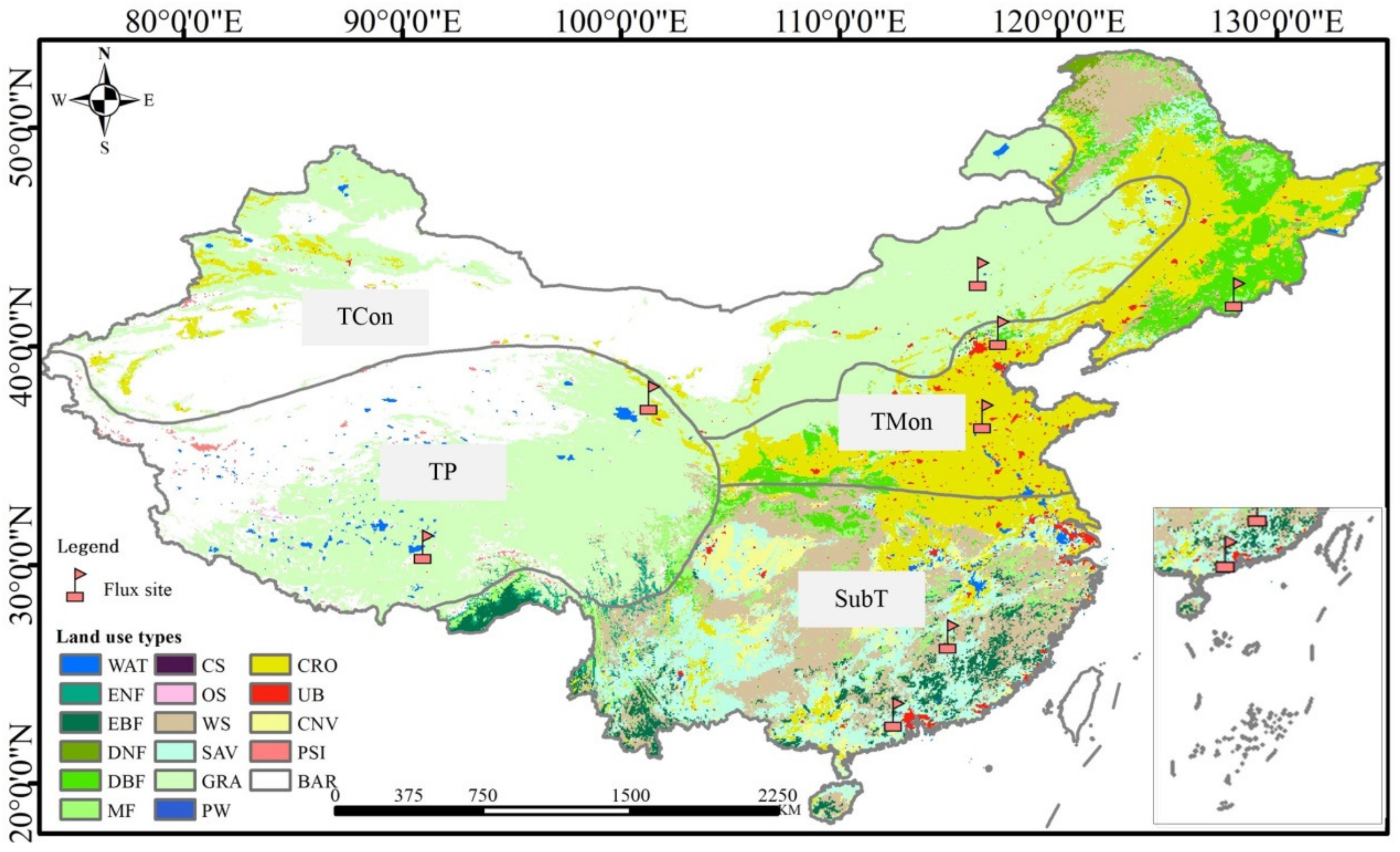
2.1. Study Area

China has been undergoing significant vegetation restoration over the past 30 years. In particular, only 6.6% of the global vegetated area alone accounted for 25% of the global net increase in leaf area index (LAI) during 2000–2017 [36]. Among the climate factors, the annual precipitation and mean temperature over China showed significant increase trends of 5.05 mm yr⁻¹ and 0.025 °C y⁻¹, and the annual incoming solar radiation experienced a decreasing trend (8.56 MJ m⁻² y⁻¹) during 2001–2020 [21]. Meanwhile, the annual ET has shown an evident increase trend (0.28 mm yr⁻¹) and annual runoff (−0.09 mm yr⁻¹) has shown a slight decrease trend over China since the 1980s [16]. However, it should be noted that the vegetation, climate, and hydrology variables vary noticeably in space.

2.2. Dataset

Meteorological factors (precipitation, temperature, wind speed, solar radiation, atmospheric pressure, humidity) and remote sensing data (LAI, land cover) were used to drive the remote sensing-based ecohydrological model. We employed a monthly China Meteorological Forcing Dataset (CMFD) with 0.1° between 1999 and 2018 as climatic factor inputs (https://www.tpdc.ac.cn/zh-hans/data, the last accessed data is on 28 December 2023). This dataset has been widely employed to drive model simulations and data analyses in recent years [37].

LAI data are the most important remotely sensed driver of model-based simulations. We collected the extensively used GLOBMAP V3.0 LAI products ([3,38,39,40] with 0.08° from 1999 to 2018 online (https://www.resdc.cn/data.aspx?DATAID=336, last accessed date is on 28 December 2023). The original GLOBMAP V3.0 LAI has half months in 1999 and eight-day periods between 2000 and 2018, which were composited into monthly data [41]. Annual dynamic land cover data were provided by the Moderate Resolution Imaging Spectroradiometer (MODIS) with 0.05° between 2001 and 2018 (https://modis.gsfc.nasa.gov/data/dataprod/mod12.php, last accessed date is on 28 December 2023). We adopted the International Geosphere-Biosphere Programme (IGBP) classification method, which includes 17 land-cover types. Because it begins in 2001, the corresponding land cover dataset for 1999 to 2000 was replaced with the 2001 land cover map. We used the monthly albedo calculated by white-sky and black-sky albedo.

Monthly eddy covariance (EC) records based on the latent heat and net ecosystem exchange at seven flux sites were collected from ChinaFLUX (https://www.cnern.org.cn/index.jsp, last accessed date is on 28 December 2023). The seven flux sites included Changbaishan (CBS), Inner Mongolia (NMG), Haibei (HB), Dangxiong (DX), Yucheng (YC), Qianyanzhou (QYZ), and Dinghushan (DHS). To keep the validation period constant over the seven flux sites, we used the period of 2004 to 2009 to calibrate and validate the model. The land where the flux sites were set up covered crops, forest, grass, and shrubs (

Table 1. Seven flux sites used for model validation.

Site	Location (°E, °N)	Land Cover Type	Range
CBS	128.10, 42.40	Mixed forest (MF)	2004–2009
NMG	117.45, 43.50	Grass (GRA)
HB	101.32, 37.60	Shrub (SHR)
DX	91.08, 30.85	Grass (GRA)
YC	116.60, 26.95	Crop (CRO)
QYZ	115.07, 26.73	Evergreen needleleaf forest (ENF)
DHS	112.56, 23.01	Evergreen broadleaf forest (EBF)

). We used proportionality parameters [37,42] to calculate the monthly GPP and ET.

We used the spatial distribution of wheat over China [28] to minimize the uncertainty of irrigation when calculating ET. Considering the spatial resolution of the dataset, the remotely sensed LAI, albedo, and raster meteorological datasets from 1999 and 2018 were resampled to 0.05° via bilinear interpolation. Due to the deficiency of LAI data in desert and bare lands, we selected only non-desert areas in Mainland China as our study region (Figure 1).

2.3. Methodology

2.3.1. Remote Sensing-Based Ecohydrological Model

(1)

Penman–Monteith–Leuning model

In this study, the ET model includes soil evaporation (E_s: mm), plant transpiration (E_c: mm), and intercepting canopy evaporation (E_i: mm) (Equation (1)).

$$ET=E_c+E_s+E_i$$

(1)

Here, the PML model [16,24] was applied to simulate E_s and E_c. Soil evaporation (Equations (2)–(7)) and plant transpiration (Equations (8)–(12)) were calculated as follows:

$$\begin{array}{l}{E}_c=\frac{1000}{\lambda {\rho }_w}\left(\frac{\frac{s}{\gamma }{R}_{nc}+\mathrm{86,400}(\frac{\rho c_p}{\gamma })D_a{G}_a}{\frac{s}{\gamma }+1+\frac{G_a}{G_c}}\right)\\ \end{array}$$

(2)

$$R_{nc}=R_n(1-\exp (-K_{A}LAI))$$

(3)

$$R_{ns}=R_n-R_{nc}$$

(4)

$$R_n=(1-\alpha )R_s-\sigma T^4(0.34-0.14\sqrt{e_a})(1.35\frac{R_s}{R_{so}}-0.35)$$

(5)

$$G_a=\frac{k^2{u}_m}{\frac{\ln [(Z_m-d)/Z_{om}]}{\ln [(Z_m-d)/Z_{ov}]}}$$

(6)

$$G_c=\frac{g_{sx}}{k_Q}\ln \left[\frac{Q_h+Q_{50}}{Q_h\exp (-k_{Q}LAI)+Q_{50}}\right]\left[\frac{1}{1+D_a/D_{50}}\right]$$

(7)

where λ represents the latent heat of vaporization (MJ kg⁻¹); ρ_w and ρ, respectively, represent the water and air density (kg m⁻³); s and γ denote the slope of the saturated vapor pressure curve and psychrometric constant (kPa °C⁻¹); c_p represents the specific heat of air at constant pressure (MJ kg⁻¹ °C⁻¹); R_n and R_nc, respectively, represent the net radiation and net radiation absorbed by the canopy (MJ m⁻²); R_s is the incoming solar radiation (MJ m⁻² day⁻¹); a is the albedo; T is the average temperature (K day⁻¹); e_a is the actual pressure (Pa); R_so is the clear-sky radiation (MJ m⁻² day⁻¹); σ is the Stefan–Boltzmann constant; D_a is the vapor pressure deficit; G_a and G_c, respectively, represent the aerodynamic and canopy conductance (m s⁻¹); g_sx is the maximum stomatal conductance. In addition, K_A is the extinction coefficient for net radiation (−), k is a constant set to 0.41, u_m is the wind speed at height m (m s⁻¹), z_m represents the height of wind measurement (m), d is the zero plane displacement height (m), z_om is the roughness length governing momentum transfer, z_ov is the transfer of heat and vapor (m), Q_h is the photosynthetically active radiation at the top of the canopy (MJ m⁻² d⁻¹), and Q₅₀ and D₅₀ are the absorbed photosynthetic active radiation and the humidity deficit (MJ m⁻² d⁻¹), respectively, when the stomatal conductance is reduced to half of g_sx.

$$\begin{array}{l}{E}_s=\frac{1000}{\lambda {\rho }_w}\left(\frac{f\frac{s}{\gamma }{R}_{ns}}{\frac{s}{\gamma }+1}\right)\\ \end{array}$$

(8)

$$f=\min (\frac{1.2P}{E_{seq}},1)$$

(9)

$$E_{seq}=\frac{A\frac{s}{r}}{\lambda \left(1+\frac{s}{r}\right)}$$

(10)

$$A=R_n-G$$

(11)

$$G=0.07\left(T_{i+1}-T_{i-1}\right)$$

(12)

where P is the monthly average rainfall (mm) and f is the ratio of soil evaporation (0–1). We set f to 1 from March to May for winter wheat lands due to irrigation [43]. E_seq is calculated by Equation (9); G denotes soil heat flux (MJ m⁻²) and can be estimated by Equation (11) [44]; and T_i+1 and T_i−1, respectively, reference the average atmospheric temperatures in prior and subsequent months (°C).

In addition, we used a modified van Dijk model [45,46,47] to calculate E_i by the canopy, and the detailed equations can be found in [47].

(2)

LUE model

We used the GPP calculation process of the Global Production Efficiency model [48,49] to simulate the spatiotemporal changes in GPP over the study area. The GPP equations simultaneously consider water and temperature stress.

$$GPP=\epsilon \cdot IPAR\cdot f(T)\cdot f(\beta )$$

(13)

$$IPAR=\alpha R_s(1-e^{k_{Q}LAI})$$

(14)

$$f(\beta )=0.5+0.5\frac{ET}{E{T}_p}$$

(15)

$$f(T)=\frac{(T_{ava}-T_{\min })-(T_{ava}-T_{\max })}{(T_{ava}-T_{\min })(T_{ava}-T_{\max })-(T_{ava}-T_{opt})(T_{ava}-T_{opt})}$$

(16)

where ε represents LUE (g C MJ⁻¹); IPAR is the amount of PAR absorbed by the plant (MJ m⁻²); f(T) and f(B), respectively, reference strict functions of temperature and water; T_ava denotes the monthly average air temperature (°C); T_opt denotes the optimum temperature (°C) at which the maximum photosynthesis is performed; and T_min and T_max, respectively, represent the extreme temperatures (°C) at which photosynthesis is terminated. R_s is the monthly total solar radiation (MJ m⁻² month⁻¹), and a is the ratio of PAR and R_S.

We also used the FAO P-M function [50] to calculate the monthly reference ET [41].

2.3.2. Optimization and Evaluation of Model Parameters

The g_sx in the ET model and ε in the LUE model act as the most sensitive parameters for regional ET and GPP simulations [27,41]. We used the aforementioned flux sites and the coefficient of determination (R²), root mean square error (RMSE), and Nash–Sutcliffe efficiency (NSE) to optimize these two parameters and further improve the model performance. The final, optimized parameters are shown in

Table 2. Optimized parameter values for different land cover types.

Model	Parameter	ENF	EBF	DNF	DBF	MF	SHR	GRA	CRO	CNV
ET	gsx	0.005	0.003	0.005	0.005	0.006	0.005	0.008	0.009	0.009
LUE	ε	1.43	0.75	1.31	1.30	1.34	1.18	1.21	2.69	2.69

.

R², RMSE, and NSE are widely employed to characterize the accuracy of geoscientific analyses [6,21,51]. We used these three indexes to evaluate our model’s performance.

$$R^2={\left(\frac{{\displaystyle \sum _{i=1}^t\left(x_i^{obs}-x_i^{\overline{obs}}\right)\left(x_i^{sim}-x_i^{\overline{sim}}\right)}}{\sqrt{{\displaystyle \sum _{i=1}^t{\left(x_i^{obs}-x_i^{\overline{obs}}\right)}^2}}\sqrt{{\displaystyle \sum _{i=1}^t{\left(x_i^{sim}-x_i^{\overline{sim}}\right)}^2}}}\right)}^2$$

(17)

$$NSE=1-\frac{{\displaystyle \sum _{i=1}^t{(x_i^{obs}-x_i^{sim})}^2}}{{\displaystyle \sum _{i=1}^t{(x_i^{obs}-x_i^{\overline{obs}})}^2}}$$

(18)

$$RMSE=\sqrt{\frac{1}{t}{\displaystyle \sum _{i=1}^t{(x_i^{obs}-x_i^{sim})}^2}}$$

(19)

where x^obs and x^sim are, respectively, the measured and modeled ET or GPP; $x^{\overline{obs}}$ and $x^{\overline{sim}}$ are the averages of the measured and modeled ET or GPP, respectively; and t is the sample count.

2.3.3. Attribution Method

We used the residual trend method [15] to identify vegetation changes disturbed by climate factors and anthropogenic activities as they affect ET and GPP.

The residual trend method is a pixel-wise operation based on the positive correlation between the LAI and precipitation in ecosystems. To carry out the residual trend method, the regression equation (Equation (20) was used to compute the pixel-by-pixel predicted LAI for every year. Then, Equations (21) and (22) were, respectively, used to estimate the slope and intercept of the curve. The intercept of the regression represents the theoretical LAI when rainfall is zero. The predicted LAI highlights the climatic impacts on the LAI. However, the observed LAI is indicative of the impacts of both humans and the climate on the LAI. The residual LAI was obtained by subtracting the observed LAI from the predicted LAI.

$$y=X\stackrel{\wedge }{\beta }+b$$

(20)

$$\stackrel{\wedge }{\beta }=\frac{n({\displaystyle \sum Xy})-({\displaystyle \sum X})({\displaystyle \sum y})}{n{\displaystyle \sum X^2}-{({\displaystyle \sum X})}^2}$$

(21)

$$c=\overline{y}-\stackrel{\wedge }{\beta }\overline{X}$$

(22)

where y is the dependent variable; X is the independent variable; $\stackrel{\wedge }{\beta }$ is the slope of the regression; and c is the intercept.

This involved first dividing the actual LAI into three components: the LAIC induced by climate, the LAIH disturbed by human activities, and a negligible residual. Variations in vegetation due to human activities were characterized by the actual LAI minus LAIC [6]. Then, we used ridge regression to identify the contributions of climatic factors and anthropogenic activities to variations in ET and GPP.

The regression function can generally be described as Equation (20), and the least square method can be used to estimate the regression coefficient $\stackrel{\wedge }{\beta }$; see Equation (23).

$$\stackrel{\wedge }{\beta }={(X^{\prime }X)}^{-1}{X}^{\prime }y$$

(23)

The interactions between climatic and human activity factors can generate multi-collinearity effects, which can result in X′X ≈ 0. Then, the variance of the unbiased estimate will be large, leading to unstable estimation. Ridge regression can add a small disturbance λI to the least square function to address the situation wherein the generalized inverse value cannot be found (Equation (24)).

$$\stackrel{\wedge }{\beta }(k)={(X^{\prime }X+\lambda I)}^{-1}{X}^{\prime }y$$

(24)

Ridge regression has been proven to be a useful resolution to eliminate collinearity effects among independent variables [10]. This is a roughly four-step process.

(1)

Each driving variable is normalized to avoid the influence of units and values.

(2)

The standard ridge regression coefficients of ET and GPP to each variable are obtained.

(3)

The standard ridge regression coefficient and trends of variables are combined to calculate the contributions of each driving factor:

$${\eta }_{ci}=a_i\cdot X_{is\_trend}$$

(25)

where i is the number of driving factors, ${\eta }_{ci}$ denotes the contributions of the normalized driving factor to the normalized trend of ET or GPP, and X_{is_trend} denotes the trend of the normalized driving factor.

(4)

Based on the trends and contributions of each normalized and actual driving factor, the relative and actual contributions of each controlling factor on ET or GPP variations are calculated as follows:

$$\begin{array}{l}{\eta }_{rci}=\frac{\left|{\eta }_{ci}\right|}{\left|{\eta }_{c1}\right|+\left|{\eta }_{c2}\right|+\left|{\eta }_{c3}\right|+\cdot \cdot \cdot }\\ \end{array}$$

(26)

$${\eta }_{aci}=\frac{{\eta }_{ci}}{Y_{s\_trend}}\cdot Y_{trend}$$

(27)

where i is the number of driving factors; ${\eta }_{rci}$ and ${\eta }_{aci}$, respectively, represent the relative and actual contributions of X_i to the trend of ET or GPP; Y_{s_trend} denotes the normalized ET or GPP trend; and Y_trend denotes the actual trend of ET or GPP.

Finally, we used the Sen’slope method [52] to determine the trends of the actual and normalized variables and examined the trend significance with a Mann–Kendall statistical test [53].

3. Results

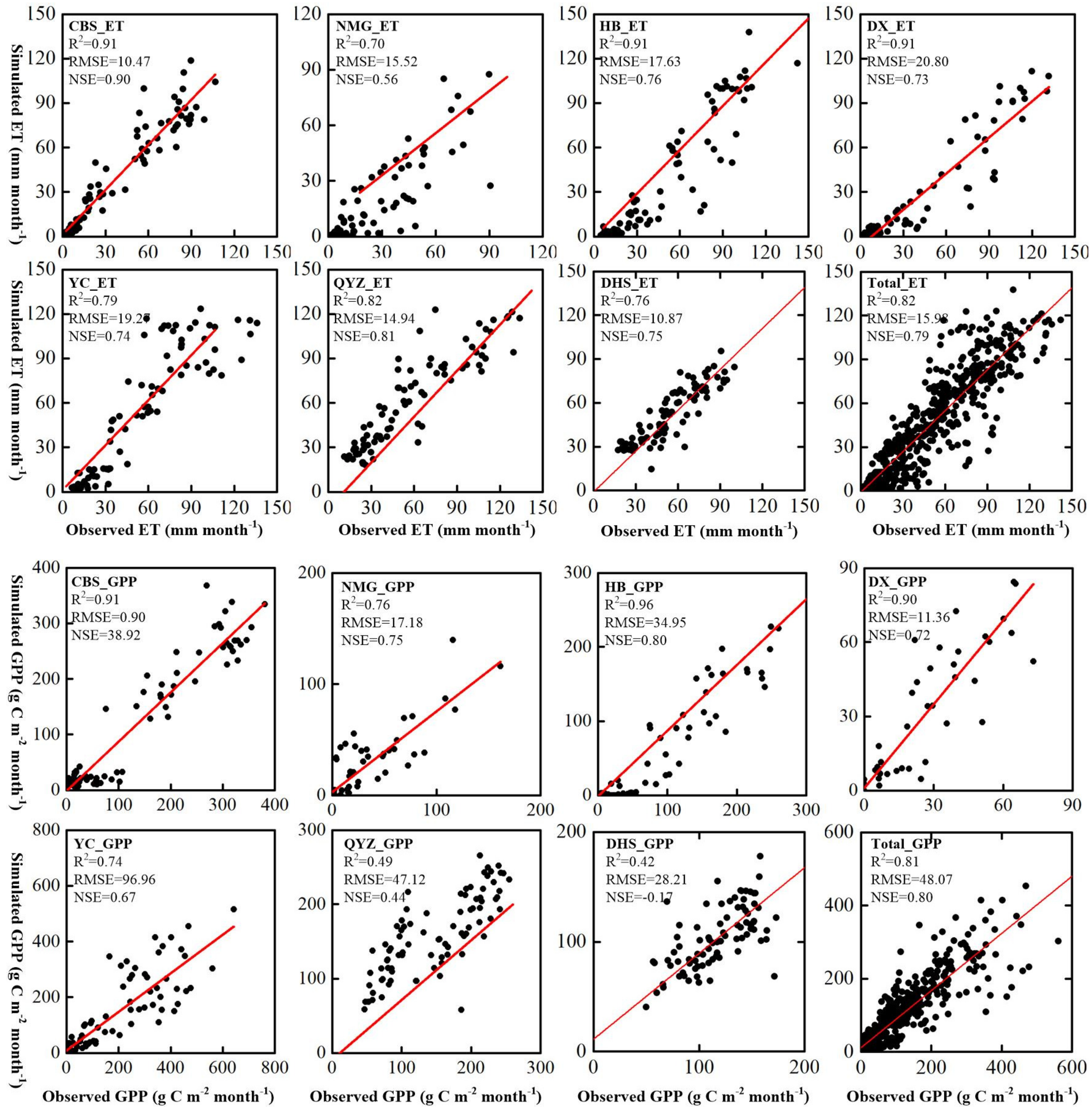
3.1. Evaluation of Simulated ET and GPP

Figure 2 displays the evaluation conditions of the modeled ET and GPP in this study versus the 72 ET and GPP observational records from seven flux sites (Figure 1) between 2003 and 2009. The R², RMSE, and NSE values shown in Figure 2 indicate that the constructed remote sensing-based ecohydrological model accurately simulates the ET over China. For example, the R² of the simulated monthly ET based on the total records in seven flux sites is 0.82; the RMSE is 15.98 mm month⁻¹ and the NSE is 0.79 by comparison against the observed ET. Interestingly, different land covers perform differently. For the three forest field sites (DHS, QYZ, and CBS), the RMSEs, R²s, and NSEs, respectively, range from 10.47 mm month⁻¹ to 14.94 mm month⁻¹, from 0.76 to 0.91, and from 0.75 to 0.90. The CBS site outperforms the others. For the two grass fields (NMG and DX), the RMSEs, R²s, and NSEs are 15.52 mm month⁻¹ and 20.80 mm month⁻¹; 0.70 and 0.91; and 0.56 and 0.73, respectively. The DX site has better performance than NMG. The shrubland site (HB) and cropland (YC) also perform well as per their R² values of 0.91 and 0.79, NSE values of 0.76 and 0.74, and RMSE values of 17.63 mm month⁻¹ and 19.21 mm month⁻¹, respectively.

In addition to ET, the total GPP was also simulated accurately, with an R² of 0.81, RMSE of 48.07 g C m⁻² month⁻¹, and NSE of 0.80 (Figure 2). Among the forest sites, CBS still outperforms QYZ and DHS, with an R² of 0.91, RMSE of 38.92 g C m⁻² month⁻¹, and NSE of 0.90. For grassland sites, DX still outperforms NMG (R² 0.90 vs. 076, RMSE 11.36 g C m⁻² vs. 17.18 g C m⁻², and NSE 0.72 vs. 0.75). The shrubland site (HB) also has an accurate GPP, with an R² of 0.96, RMSE of 34.95 g C m⁻² month⁻¹, and NSE of 0.80. Compared with other vegetation types, although the cropland site (YC) has a larger RMSE of 96.96 g C m⁻² month⁻¹, it still presents good consistency (R² of 0.74 and NSE of 0.67). The general consistency between the simulations of the three validation indicators and the EC observations suggests that the proposed model is accurate enough to support our subsequent analyses.

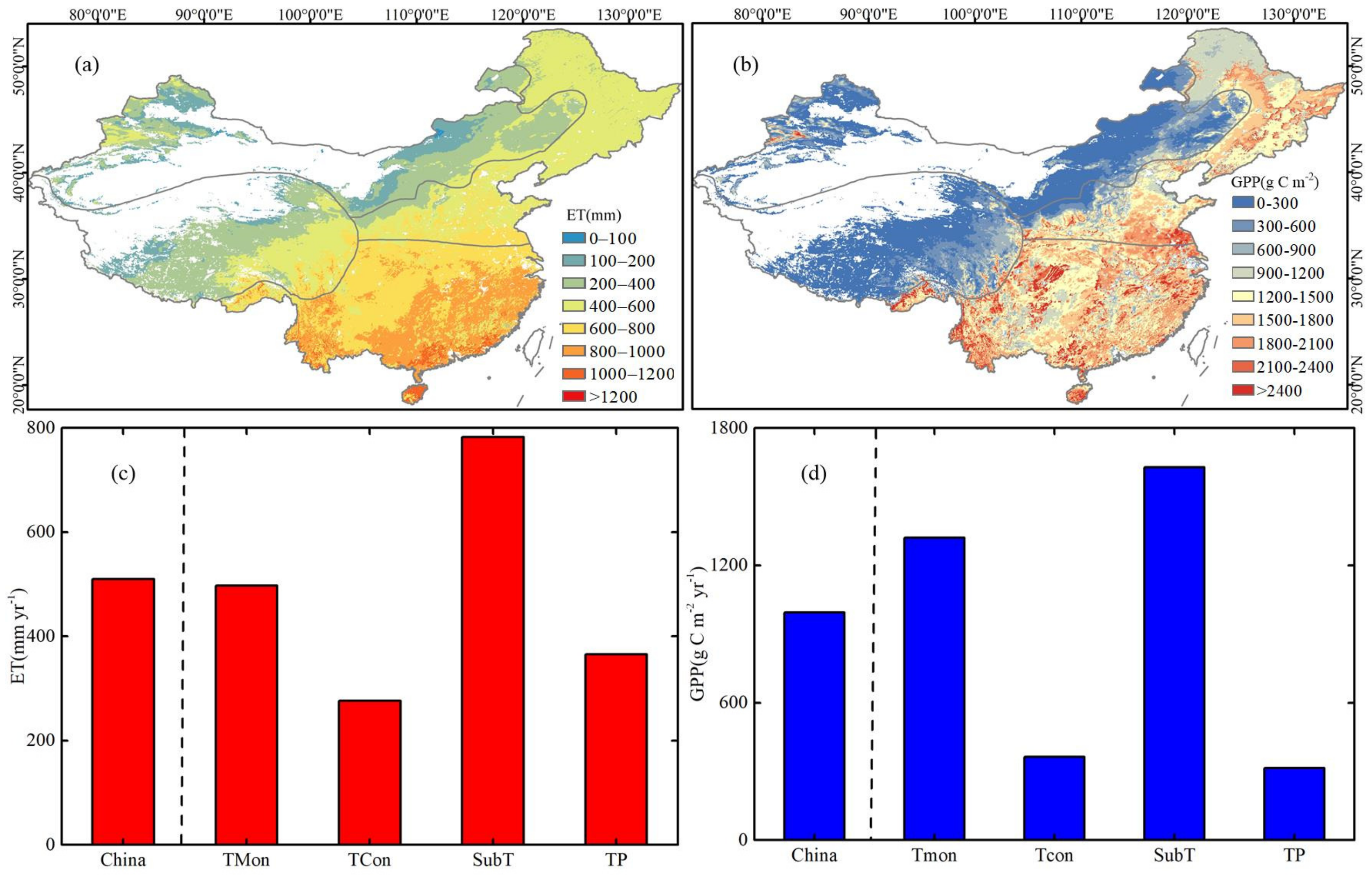
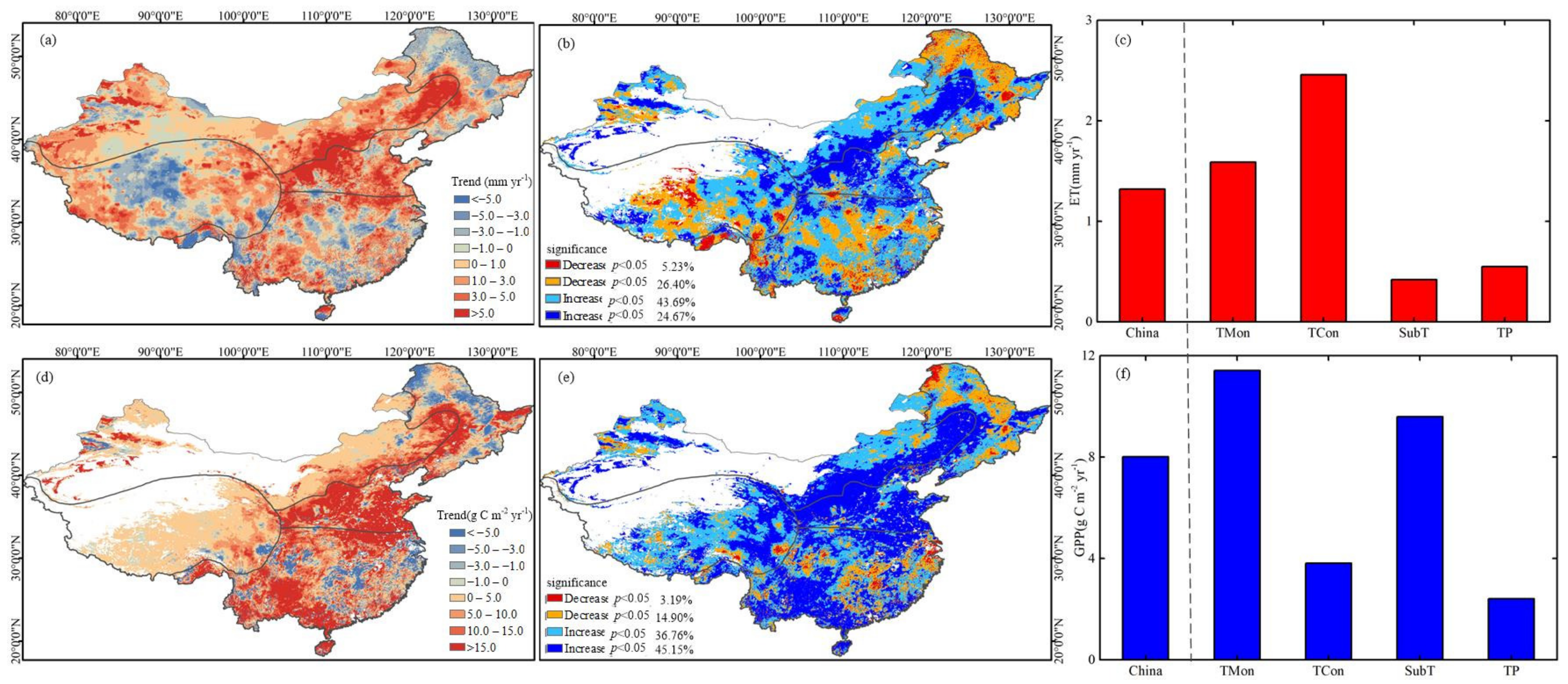
3.2. Spatiotemporal Trends of ET and GPP

Figure 3a,b show the consistent spatial patterns of the annual average ET and GPP, with an increasing trend from northwest to southeast over Mainland China and a range from lower than 100 mm (lower than 300 g C m⁻² yr⁻¹) to more than 1200 mm (2400 g C m⁻² yr⁻¹) for ET (GPP). As shown in Figure 3c,d, ET and GPP differ significantly by region, ranging from 276.41 mm yr⁻¹ over TCon to 782.29 mm yr⁻¹ over SubT (from 314.49 g C m⁻² yr⁻¹ over TP to 1628.61 g C m⁻² yr⁻¹ for SubT).

The annual average ET and GPP over China in this study are, respectively, 510.11 mm and 994.55 g C m⁻² between 1999 and 2018. Previous studies show that the vegetated Mainland China’s annual ET value averaged from 2001 to 2020 is 409.05 mm [21], the national average annual ET and GPP are, respectively, about 475 mm and 1120 g C m⁻² between 2000 and 2017 [6], the vegetated annual ET over China from 2002 to 2016 is 534.7 ± 232.8 mm yr⁻¹ based on eddy covariance measurements [54], the total GPP over China’s terrestrial ecosystem is 6.80 P g C yr⁻¹ between 1999 and 2015 using the model tree ensemble algorithm, and the total GPP in this study is 6.88 P g C yr⁻¹ [19]. The simulated results of ET and GPP in this study are reasonable based on the previous studies.

Figure 4 shows the trend values and significance levels of ET and GPP over Mainland China, as well as statistical trends for the four sub-regions between 1999 and 2018. Figure 4a,b show that the ET increases over more than 68% of the study area; the area ratio of significant (p < 0.05) increasing trends over China is 24.67%. The most intense trends (>5 mm yr⁻¹) are mainly distributed in Central, Northeastern, Western, and Southeastern China. The spatial patterns of the increases in GPP are similar to those of ET. The most intense GPP trends (>15 g C m⁻² yr⁻¹) are mainly in Central, Northeastern, and Southwestern China (Figure 4d). More than 43% of the study area shows significant (p < 0.05) upward trends (Figure 4e). The statistical results in Figure 4c,f show increasing ET (GPP) trends of 1.32 mm yr⁻¹ (8.01 g C m⁻² yr⁻¹) over vegetated Mainland China. The four sub-regions also show increasing trends for ET (GPP); TCon (TMon) has the strongest increasing trend of 2.46 mm yr⁻¹ (11.42 g C m⁻² yr⁻¹), while SubT (TP) has the weakest increasing trend of 0.42 mm yr⁻¹ (2.41 g C m⁻² yr⁻¹).

3.3. Trends of Climate Factors and Vegetation

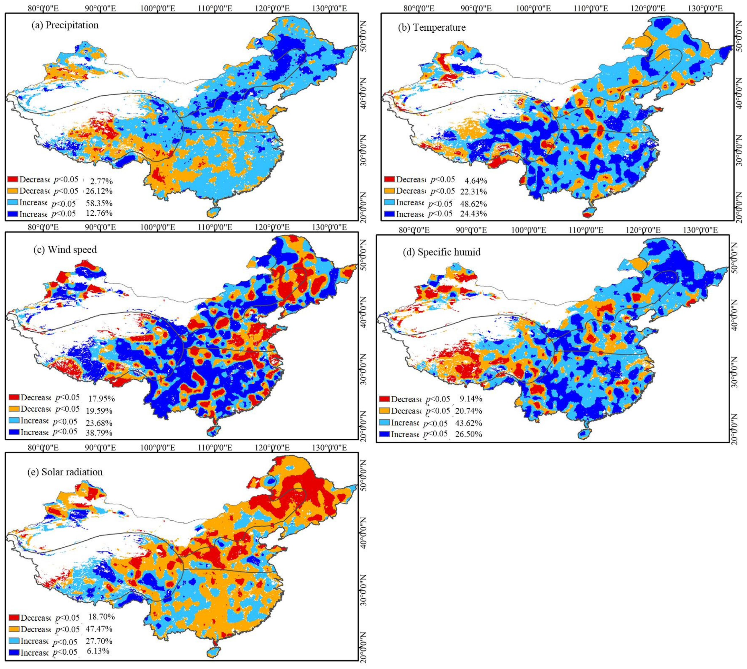
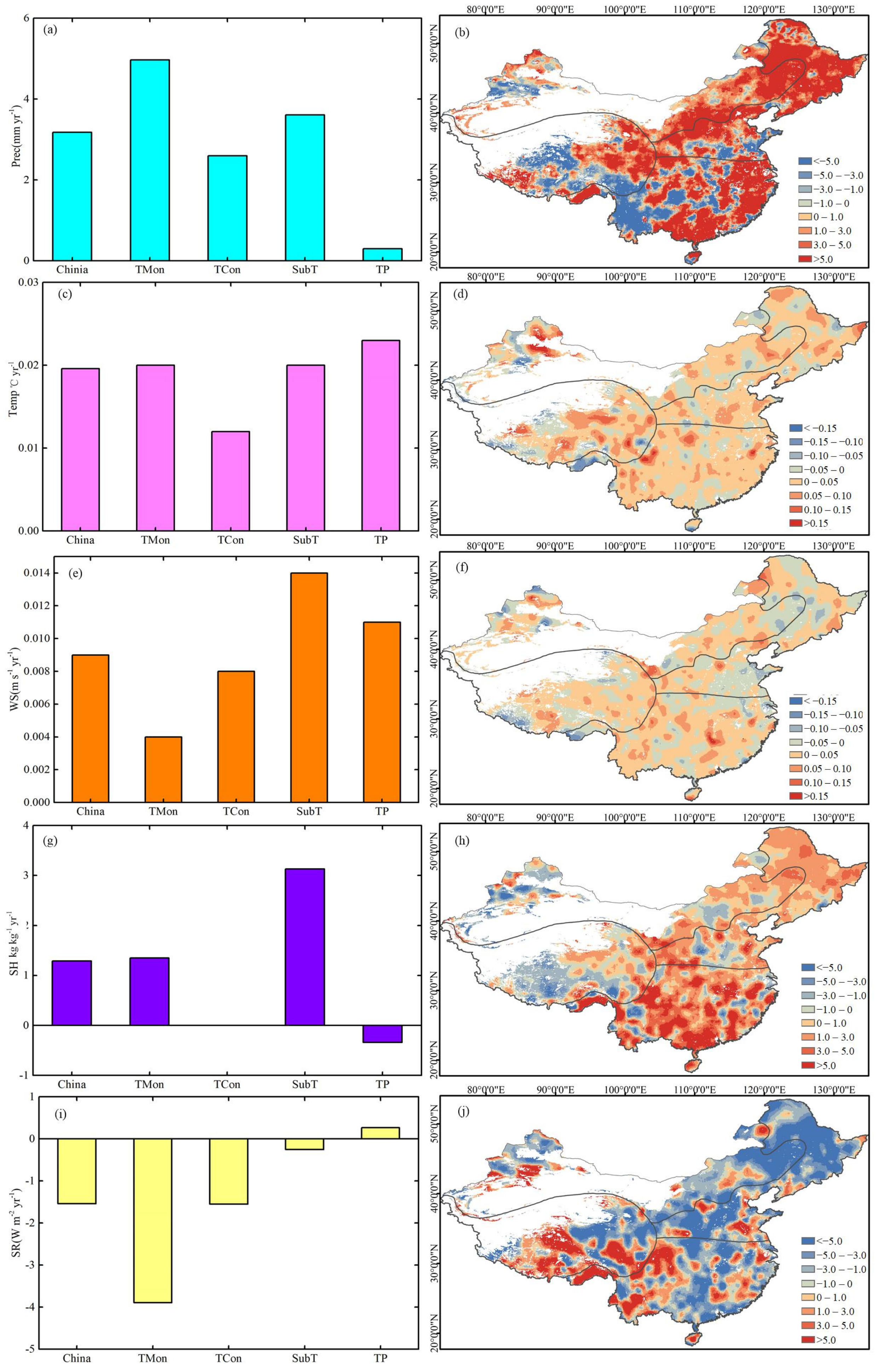
3.3.1. Trends in Climate Factors

Figure 5 and Figure A1 show the spatial distributions of trends and trend significance for five climatic factors over China, as well as statistical trends in sub-regions, from 1999 to 2018. Precipitation shows an upward trend of 3.18 mm yr⁻¹ over China (Figure 5a). The most significant trends (>5 mm yr⁻¹) are distributed in the eastern parts of China (Figure 5b), and 12.76% of regions (primarily in Northeastern and Central–Western China) undergo significant (p < 0.05) increases (Figure A1a). Among the four sub-regions, TMon and TP have the most and least intense trends, with values of 4.97 mm yr⁻¹ and 0.30 mm yr⁻¹, respectively (Figure 5a).

Mainland China shows a warming mean temperature trend of 0.020 °C yr⁻¹ (Figure 5c,d). Spatially, 24.43% of the regions (primarily in Southwestern, Northern, and Southeastern China) experienced significant (p < 0.05) increases (Figure A1b). Among the four sub-regions, TP and TCon show the most (0.023 °C yr⁻¹) and least (0.012 °C yr⁻¹) significant trends (Figure 5d).

The overall trend in wind speed over Mainland China from 1999 to 2018 is 0.010 m s⁻¹ (Figure 5e). More than 73% of China experienced increasing wind speeds, and 38.798% of regions (primarily in Southwestern and Southeastern China) show significant (p < 0.05) increases (Figure 5f and Figure A1c). Among the four sub-regions, SubT and TMon show the most (0.014 m s⁻¹) and least (0.004 m s⁻¹) significant trends (Figure 5e).

Although the specific humidity over China has a slightly positive trend (1.29 × 10⁻⁵ kg kg⁻¹ yr⁻¹), particularly in SubT (3.13 × 10⁻⁵ kg kg⁻¹ yr⁻¹), TCon has a trend of 0 and TP has a negative trend of −0.34 × 10⁻⁵ kg kg⁻¹ yr⁻¹ (Figure 5j). Spatially, the most significant increasing trends are distributed over Southern China, and 26.50% of the areas show significant (p < 0.05) increases.

Unlike other climate factors, solar radiation decreases over the whole of China (−1.54 W m⁻² yr⁻¹) from 1999 to 2018 (Figure 5i). Only TP has a slightly increasing value (0.27 W m⁻² yr⁻¹); TMon, TCon, and SubT have decreasing trends of −3.89 W m⁻² yr⁻¹, −1.55 W m⁻² yr⁻¹, and −0.25 W m⁻² yr⁻¹, respectively (Figure 5i). Spatially, the most significant increasing trend is distributed over Southwestern China, while only 6.13% of the areas have significant (p < 0.05) increases. The area with significant (p < 0.05) decreasing trends accounts for 18.70%, mainly in the central and northeastern parts of the country.

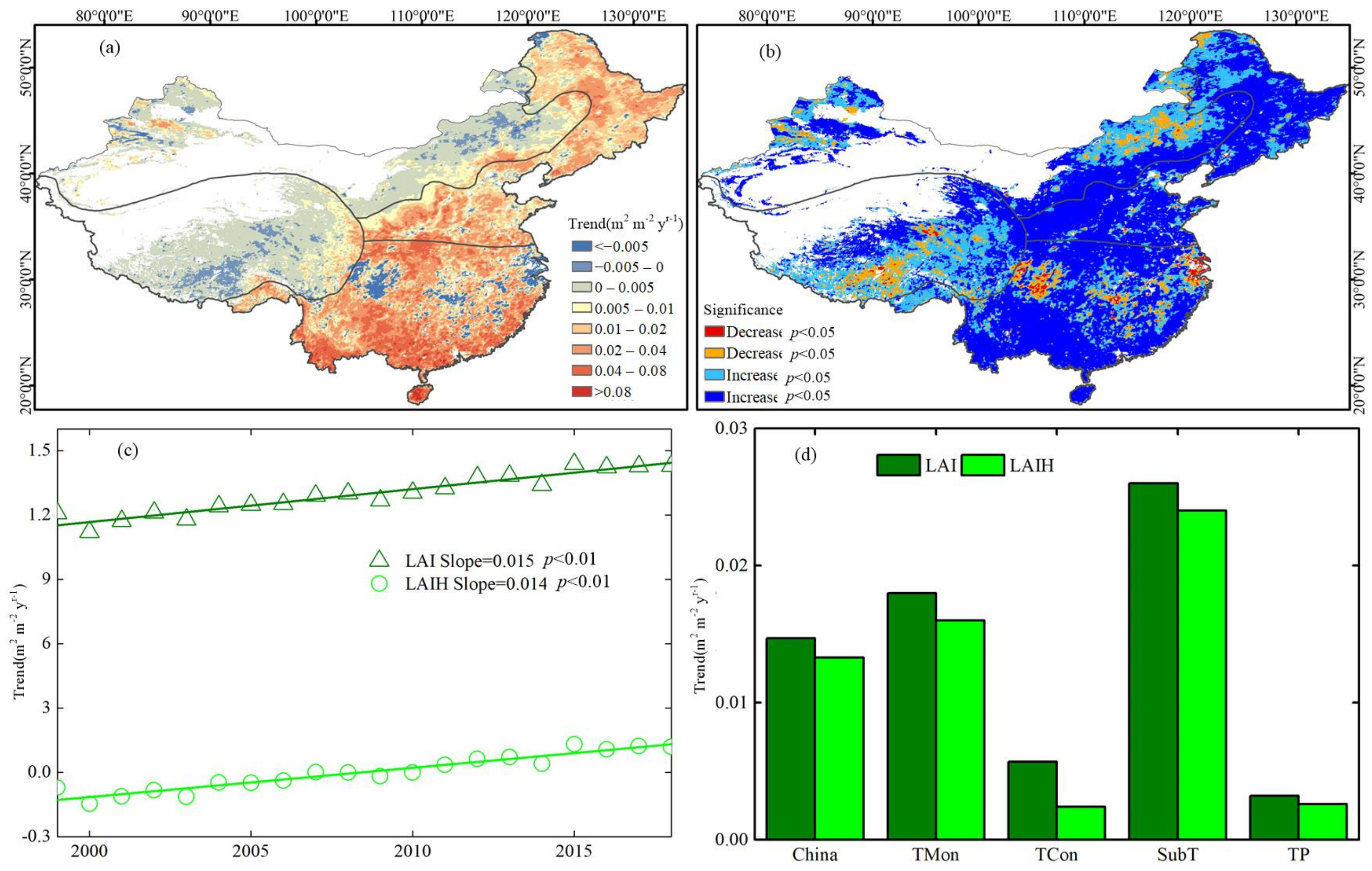
3.3.2. Trends in Vegetation

Figure 6a,b, respectively, show the spatial patterns of the LAIH trend values and significance over Mainland China between 1999 and 2018. The LAIH shows increasing trends across more than 90% of China. The area ratio of significant (p < 0.05) increasing trends over China is more than 70%. The most intense trends (>0.01 yr⁻¹) are mainly distributed in Central and Southern China. On average, both the actual LAI and LAIH driven by human activities over China significantly increase, at 0.015 and 0.014 (p < 0.001) during 1999–2018 (Figure 6c). Anthropogenic activities have dominant effects on vegetation restoration. Compared to the positive trends of the actual LAI, the temporal trends of the LAIH change from negative to positive in the year 2010 (Figure 6c). Among the four sub-regions, SubT shows the highest increase rates of 0.026 yr⁻¹ and 0.024 yr⁻¹ for the LAI and LAIH; TP has the lowest increase rates of 0.0032 yr⁻¹ and 0.0026 yr⁻¹ for the LAI and LAIH, respectively (Figure 6d).

From the perspective of the spatial distribution of the LAIH trend (Figure 6a), there are significantly positive LAH trends in the west of TMon and northwest of SubT due to the implementation of the “Grain for Green Program”. The evident positive LAIH trend in the southwest of TCon is attributed to the implementation of the “Rocky Desertification Integrated Management” scheme. The “Three-North Forest Shelterbelt Program” is an important factor causing positive changes in the LAIH in the north of TMon.

3.4. Identification of Factor Attributions for Variations in ET and GPP

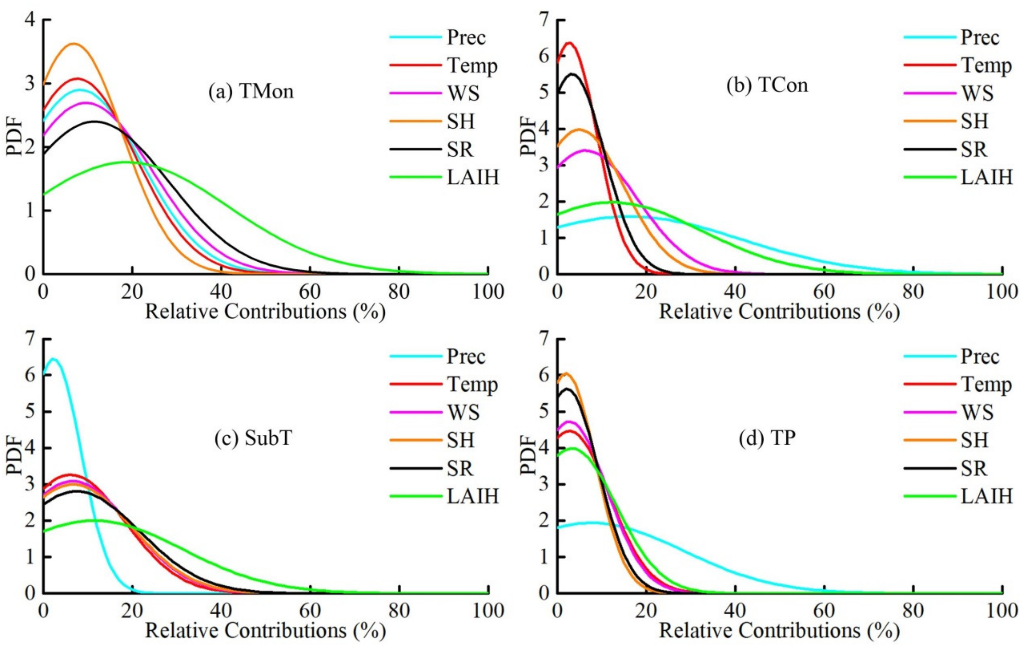
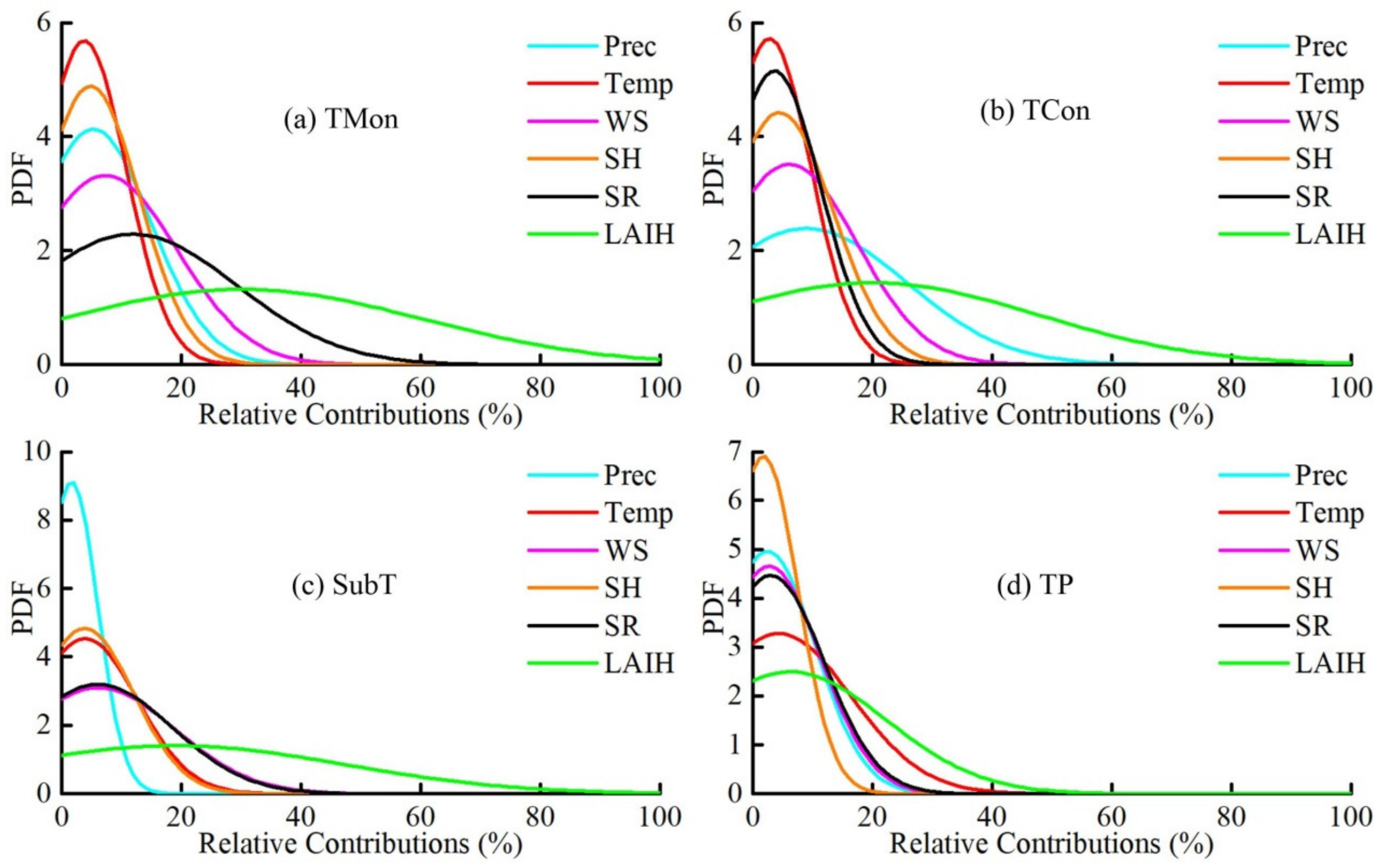
3.4.1. Relative Contributions of Influencing Factors

Figure 7 and Figure 8, respectively, show the probability density functions (PDFs) of the relative contributions of climatic factors and anthropogenic activities to the variations in ET and GPP in the four sub-regions of China.

Table 3. Mean relative contributions of influencing factors to ET and GPP variations for four sub-regions (%). TMon, TCon, SubT, and TP, respectively, represent temperate monsoonal, temperate continental, subtropical–tropical monsoonal, and high–cold Tibetan Plateau regions. Prec, Temp, WS, SH, SR, LAIH, respectively, represent precipitation, temperature, wind speed, specific humidity, solar radiation, and LAI disturbed by human activities.

		Prec	Temp	WS	SH	SR	LAIH
TMon	ET	13.78	12.26	14.78	11.02	18.42	29.72
	GPP	8.84	5.97	10.87	7.70	18.85	47.75
TCon	ET	36.84	5.64	13.27	10.65	7.19	26.33
	GPP	20.79	5.92	12.52	9.61	7.69	43.39
SubT	ET	5.73	15.15	15.79	16.43	18.37	28.50
	GPP	4.15	9.67	14.35	9.42	14.84	47.55
TP	ET	38.59	13.46	12.73	9.29	10.16	15.78
	GPP	12.43	21.53	12.29	8.47	14.39	30.90

lists the corresponding mean relative contribution values in the four sub-regions (%). These values are significantly different in the four sub-regions. The dominant driver of changes in ET is anthropogenic activities, with a mean relative contribution of 29.72% in TMon as a result of performing the large-scale Grain to Green Program. No mean contribution of climatic drivers is larger than 20%. Due to dry climate and vegetation restoration, both precipitation (mean relative contribution: 36.84%) and anthropogenic activities (mean relative contribution: 26.33%) are more important than other climate factors in controlling ET trends in TCon, while temperature plays the least important role, with a mean relative contribution of 5.64% due to cold weather in this sub-region. In SubT, precipitation has the lowest contribution of 5.73% due to the generally moist climate of the study area. The relative importance of other factors for ET trends in this sub-region is ranked as follows: LAIH with 28.50% > SR with 18.37% > SH with 16.43% > WS with 15.79% > Temp with 15.15%. In TP, the most important driver of ET trends is precipitation (mean relative contribution: 38.59%), followed by vegetation restoration (mean relative contribution: 15.78%) and temperature (mean relative contribution: 13.46%). The contribution of SH ranks lowest at 9.29%.

Unlike the ET identifications, the vegetation restoration induced by human activities (with a mean relative contribution of 47.75% in TMon, 43.39% in TCon, 47.55% in SubT, and 30.90% in TP) has a much greater influence on GPP changes in the four sub-regions than climate factors. For relative contributions, SR with 18.85%, precipitation with 20.79%, SR with 14.84%, and temperature with 21.53%, respectively, rank second in the TMon, TCon, SubT, and TP sub-regions; temperature with 5.97%, temperature with 5.92%, precipitation with 4.15%, and SH with 8.47% are at the lowest rank in the TMon, TCon, SubT, and TP sub-regions, respectively.

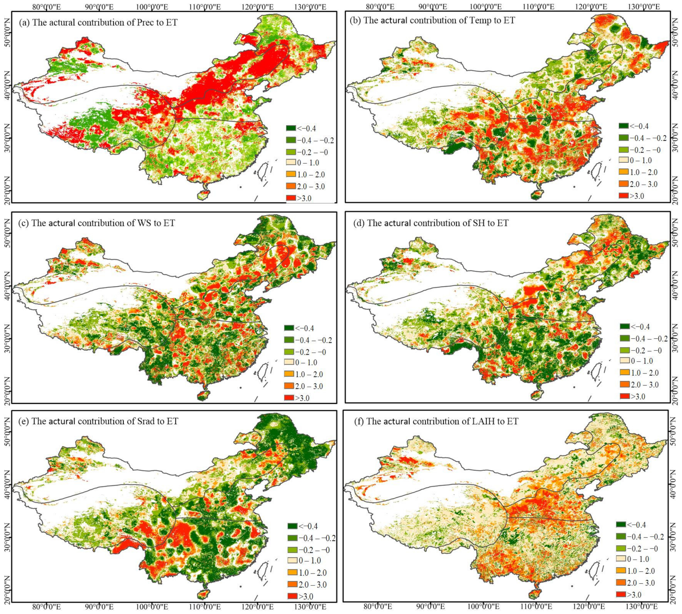
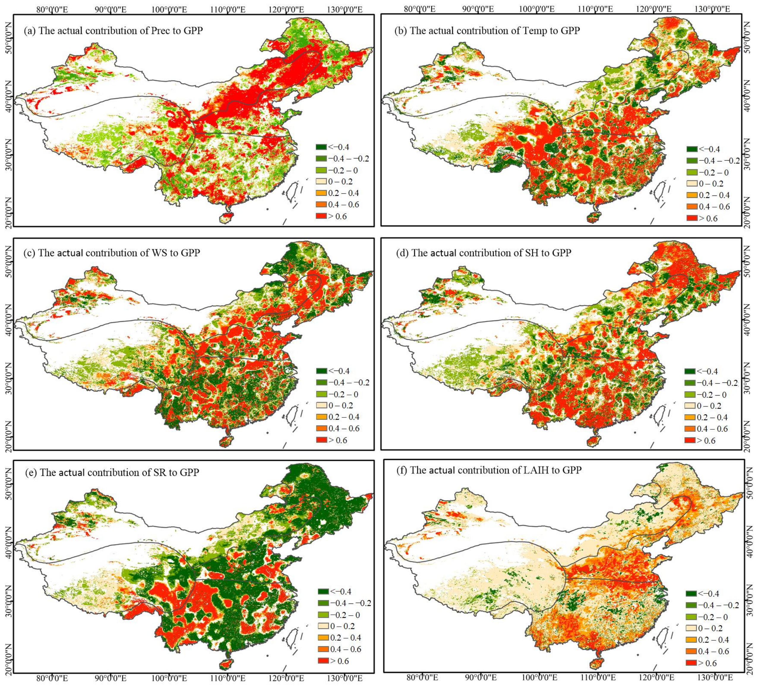
3.4.2. Actual Contributions of Influencing Factors

Although Figure 7 and Figure 8 show the relative contributions of influencing factors, they do not indicate positive or negative effects. The actual contributions calculated by Equation (27) can fill this gap. Figure 9 shows the significant spatial heterogeneity in the actual contributions of influencing factors. Precipitation has a very positive effect on ET trends in the east of TP and most of TCon, with values larger than 0.6 mm yr⁻¹. Precipitation makes a negative contribution in the middle of TP and has a slightly negative influence on most of the SubT sub-regions. As shown in

Table 4. Mean regional contributions of influencing factors to ET (mm yr⁻¹) and GPP (g C m⁻² yr⁻¹).

Sub-Region		Prec	Temp	WS	SH	SR	LAIH
TMon	ET	0.38	0.33	−0.06	−0.04	−0.62	1.12
	GPP	0.76	0.47	0.53	0.57	−2.03	7.95
TCon	ET	0.93	0.00	0.17	0.12	0.04	0.87
	GPP	1.14	0.04	0.53	0.27	−0.17	3.35
SubT	ET	0.03	0.29	−0.14	−0.39	−0.17	0.88
	GPP	0.30	0.48	0.20	0.70	−0.01	6.84
TP	ET	0.02	0.18	−0.14	−0.12	0.03	0.39
	GPP	0.18	0.46	0.09	0.00	−0.02	0.95

, precipitation has a mean positive value of 0.93 mm yr⁻¹ for TCon and 0.02 mm yr⁻¹ for TP due the offset of negative effects in the middle of TP, which indicates the higher sensitivity of ET to rainfall in TCon. The lowest-ranking negative contribution in the west of TCon and south of TMon can be attributed to the large fraction of irrigation croplands. The actual positive contribution of temperature (>0.6 mm yr⁻¹) mainly exists in the east of China and east of TP, while the west of China and most of TCon show negative effects on ET trends. In addition to TCon, the wind speed makes negative contributions in TMon, SubT, and TP, with values of −0.06 mm yr⁻¹, −0.14 mm yr⁻¹, and −0.14 mm yr⁻¹, respectively. Although SH shows a significantly positive contribution to ET in the north of TMon and southeast of SubT, TMon (−0.04 mm yr⁻¹), TP (−0.12 mm yr⁻¹), and SubT (−0.39 mm yr⁻¹) show negative contributions based on the mean actual contributions (Table 4).

The contribution of SR to ET variation is significantly positive at the Yunnan–Guizhou Plateau (Southwestern China) and has a negative effect across most of the country, which is consistent with the SH trend shown in Figure 9. Human activities make remarkably positive contributions in most of China. The value of the positive contribution is larger than 3.0 mm yr⁻¹ in the south of TMon as a result of performing the Grain to Green Program, in the southwest of SubT due to Rocky Desertification Integrated Management, and in the west of TCon due to the Returning Grazing-Growing Project. Human activities have weak effects on ET in TP, which is sparsely populated.

Figure 10 shows that the spatial distributions of the actual contributions of the influencing factors to GPP are similar to those of ET. Table 4 shows that the actual contribution ranks to GPP are different for temperature in comparison with ET. The rankings of the positive contributions of temperature to GPP are SubT (0.48 g C m⁻² yr⁻¹) > TMon (0.47 g C m⁻² yr⁻¹) > TP (0.46 g C m⁻² yr⁻¹) > TCon (0.04 g C m⁻² yr⁻¹); the rankings for ET are TMon (0.33 mm yr⁻¹) > SubT (0.29 mm yr⁻¹) > TP (0.18 mm yr⁻¹) > TCon (0.00 mm yr⁻¹). Although WS has the same rankings regarding the contributions to GPP and ET, the negative contributions over TMon, SubT, and TP are converted into positive effects. For SR and SH, there are conflicts among the ranks and types of contribution to ET and GPP. Across China, GPP is principally limited by anthropogenic activities.

4. Discussion

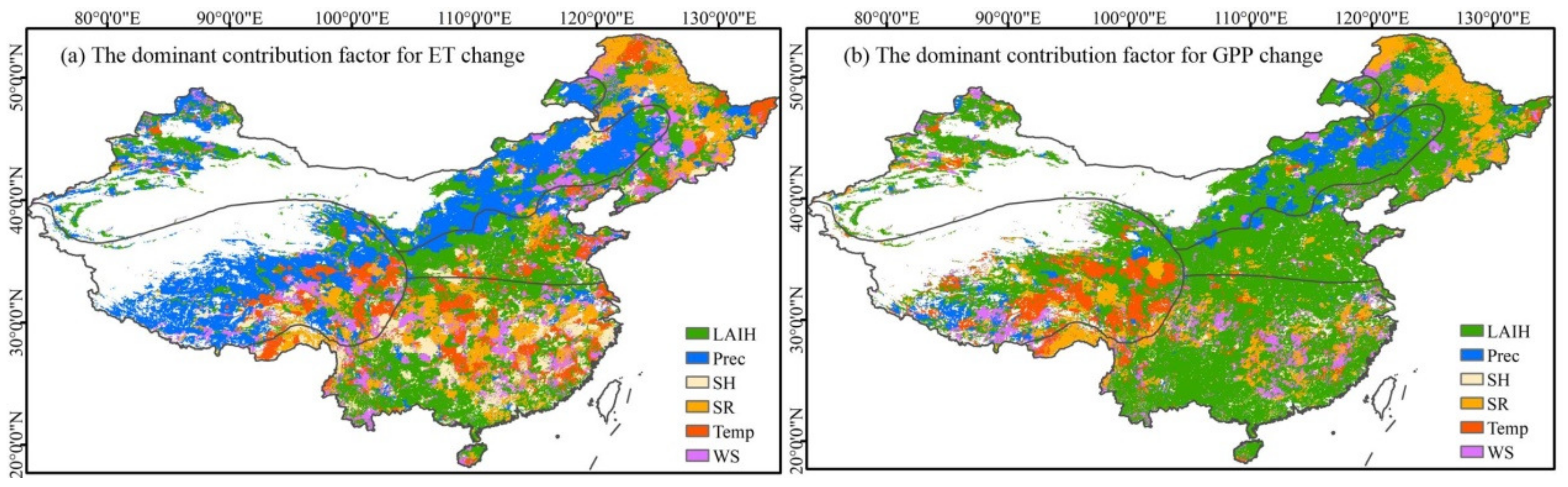
4.1. Spatial Pattern of Dominant Factors Controlling Variations in ET and GPP

According to the climatic divisions of the China Natural Geography Atlas, our study area has four sub-regions. Figure 11 shows the spatial distributions of the dominant factors controlling variations in ET and GPP over China from 1999 to 2018. Among the four sub-regions, most areas of TMon and TP have arid and semi-arid climate characteristics, and precipitation is the predominant source of water and dominates the surface ET change in these regions, which corresponds to previous findings [55,56]. Because precipitation also has an important influence on vegetation growth in semi-arid areas, it controls the increase in GPP in eastern TCon. TP mainly covers the Qinghai–Tibet Plateau, where the temperature has significantly increased and limited vegetation growth [57]. The LAIH and temperature warming together contribute significantly to regional GPP variations, while precipitation and temperature warming contribute more to regional ET variations.

Humid and semi-arid climates are distributed in the north and south of TMon, respectively. ET and GPP in northern TMon significantly decrease due to a significant decrease in SR. Southwestern TMon, namely the Loess Plateau, is the core district for the implementation of the Grain for Green Program (GFGP). Intensive vegetation restoration significantly controls the increases in LAIH, ET, and GPP in this region [10,58,59].

The SubT region, conversely, is located in Southern China, which is characterized by high temperatures and sufficient precipitation. Figure 11 shows that SR significantly influences the ET and GPP variations in this region [60,61]. The decreasing SR in the middle of TMon induces decreases in ET and GPP. Vegetation dominates the increases in ET and GPP in southwestern TMon (the Yunnan–Guizhou Plateau) due to the extensive implementation of Rocky Desertification Integrated Management. Previous researchers determined that the influence of SW on ET changes decreases from arid to humid regions [62,63,64]. The results shown in Figure 11 also support this observation.

4.2. Influences of Anthropogenic Activities on ET and GPP Trends

Vegetation greening has an important effect on ET and GPP trends over China [6,10,16,21]. The residual method was employed to produce the time-series LAIH driven by human activities in this study. Figure 6 shows where the LAIH over China significantly increases, with trends of 0.014 (p < 0.001) from negative to positive, during 1999–2018. The LAIH also spatially increases from the northwest to southeast, especially in the Loess Plateau and Yunnan–Guizhou Plateau, as likewise observed by previous researchers [65,66].

Vegetation greenness is the dominant factor in GPP, rather than climate factors [6], which we also found to be the case in this study (Figure 11). In fact, the LAI influences GPP mainly by controlling the amount of solar radiation absorbed [67]. The controlling mechanism of the LAI on ET is more complex. An increased LAI not only accelerates vegetation transpiration, but also hinders sunlight penetration and thus inhibits vegetation transpiration [68,69]. ET variations are more affected by the water supply and atmospheric evaporation water, in addition to vegetation, than GPP [70]. In areas with a significantly increasing LAI, such as Northeastern and Southern China, climate factors have a more significant effect on ET variations than anthropogenic activities.

4.3. Policy Implications

Over the past 20 years, China has performed extensive vegetation restoration programs (e.g., he Three-North Forest Shelterbelt Program, Grain for Green Program, and Rocky Desertification Integrated Management), which have increased the greenness over China, mitigated carbon accumulation, and reversed the deteriorated ecology [71]. However, when a large amount of cropland and bareland becomes grassland or forestland, ecological water consumption also increases. Compared to crops or grass, the water consumption of forests is significantly more effective due to the longer transpiration periods and deeper root lengths of plants [72]. However, China is experiencing a serious drought, which has potential contradictions for the supply and demand of water. Water-saving measures should be prioritized when enacting reforestation policies.

4.4. Uncertainties

In this study, the PML model and LUE model were coupled to simulate spatiotemporal variations in ET and GPP at the national scale between 1999 and 2018. Long-time-series, remotely sensed LAI, Albedo, and meteorological factors were employed as inputs. The parameters of the constructed model and the accuracy of the input data can create uncertainties in the simulation results. We optimized the model parameters based on 72 EC observed records from seven flux sites, but the spatial distributions of the sites were sparse when compared to the entire study area, which may have influenced the accuracy of our results. Secondly, the time-series land cover began from 2001; this study applied the data in 2001 to replace the true land cover data in 1999 and 2000. In addition, we resampled the LAI with a spatial resolution of 8 km and meteorological data with a spatial resolution of 10 km to 5 km via bilinear interpolation to match the 5 km spatial resolution of land cover. Mismatching in the data and the selection of the resampling method also may have generated uncertainties [73]. Therefore, more site observation data and higher-precision driving data are needed to minimize uncertainties when modeling ET and GPP in China in future research.

5. Conclusions

In this study, we constructed a remote sensing-based ecohydrological model to simulate the spatiotemporal changes in monthly ET and GPP between 1999 and 2018 over Mainland China. We quantitatively identified the contributions of climate factors (precipitation, temperature, wind speed, humidity, and solar radiation) and the LAI influenced by anthropogenic activities acting on ET and GPP variations. The model performance was satisfactory based on several evaluation indexes at the flux sites. Both interannual ET and GPP showed significant upward trends of 1.32 mm y⁻¹ and 8.01 g C m⁻² yr⁻¹. Four sub-regions experienced increasing trends for ET (GPP). TCon (TMon) had the strongest increasing trend of 2.46 mm yr⁻¹ (11.42 g C m⁻² yr⁻¹), while SubT (TP) had the weakest increasing trend of 0.42 mm yr⁻¹ (2.41 g C m⁻² yr⁻¹). Precipitation, temperature, wind speed, and humidity showed increasing trends over China, while solar radiation markedly decreased.

Compared with climate factors, vegetation changes due to anthropogenic disturbance significantly increased over our observation period. Based on our ridge regression results, vegetation changes due to anthropogenic activities make a dominant contribution to GPP variations; the dominant factor influencing ET changes differs in each sub-region due to the joint influences of climate and vegetation on ET. We find that human activities have an important impact on ET and GPP variations, particularly in terms of vegetation greening. Careful attention should be paid to water conservation for the sustainable development of the Chinese economy and society in enacting ecological restoration policies nationally. Meanwhile, we can collect more observations to validate the reasonability of the model simulation and higher-precision inputs to decrease the model uncertainties of ET and GPP in China in the future.

References

1. Jiang, P.; Ding, W.G.; Yuan, Y.; Hu, L.Q.; Ye, W.F. Identifying trend shifts in vegetation greenness in China from 1982 to 2015. Land Degrad. Dev. 2022, 33, 1434–1445. [Google Scholar] [CrossRef]
2. Niu, Z.; He, H.; Zhu, G.; Ren, X.; Zhang, L.; Zhang, K. An increasing trend in the ratio of transpiration to total terrestrial evapotranspiration in China from 1982 to 2015 caused by greening and warming. Agric. For. Meteorol. 2019, 279, 107701. [Google Scholar] [CrossRef]
3. Piao, S.; Yin, G.; Tan, J.; Cheng, L.; Huang, M.; Li, Y.; Liu, R.; Mao, J.; Myneni, R.B.; Peng, S.; et al. Detection and attribution of vegetation greening trend in China over the last 30 years. Glob. Chang. Biol. 2015, 21, 1601–1609. [Google Scholar] [CrossRef]
4. Wu, J.Z.; Zhang, J.; Ge, Z.M.; Xing, L.W.; Han, S.Q.; Shen, C.; Kong, F.T. Impact of climate change on maize yield in China from 1979 to 2016. J. Integr. Agr. 2021, 20, 289–299. [Google Scholar] [CrossRef]
5. Li, Y.; Piao, S.; Li, L.Z.X.; Chen, A.; Wang, X.; Ciais, P.; Huang, L.; Lian, X.; Peng, S.; Zeng, Z.; et al. Divergent hydrological response to large-scale afforestation and vegetation greening in China. Sci. Adv. 2018, 4, 9. [Google Scholar] [CrossRef] [PubMed]
6. Xue, Y.Y.; Liang, H.B.; Zhang, B.Q.; He, C.S. Vegetation restoration dominated the variation of water use efficiency in China. J. Hydrol. 2022, 612, 128257. [Google Scholar] [CrossRef]
7. Baldocchi, D.; Meyers, T. On using eco-physiological, micro-meteorological and biogeochemical theory to evaluate carbon dioxide, water vapor and trace gas fluxes over vegetation: A perspective. Agr. Forest Meteorol. 1998, 90, 1–25. [Google Scholar] [CrossRef]
8. Mo, X.G.; Liu, S.X.; Chen, X.J.; Hu, S. Variability, tendencies, and climate controls of terrestrial evapotranspiration and gross primary productivity in the recent decade over China. Ecohydrology 2018, 11, e1951. [Google Scholar] [CrossRef]
9. Seneviratne, S.I.; Lüthi, D.; Litschi, M.; Schär, C. Land–atmosphere coupling and climate change in Europe. Nature 2006, 443, 205–209. [Google Scholar] [CrossRef]
10. Xie, S.D.; Mo, X.G.; Hu, S.; Liu, S.X. Contributions of climate change, elevated atmospheric CO2 and human activities to ET and GPP trends in the Three-North Region of China. Agric. Forest Meteorol. 2020, 295, 108183. [Google Scholar] [CrossRef]
11. Cavalcante, R.B.L.; Pontes, P.R.M.; Souza, P.W.M.; de Souza, E.B. Opposite effects of climate and land use changes on the annual water balance in the Amazon arc of deforestation. Water Resour. Res. 2019, 55, 3092–3106. [Google Scholar] [CrossRef]
12. Katul, G.G.; Oren, R.; Manzoni, S.; Higgins, C.; Parlange, M.B. Evapotranspiration: A process driving mass transport and energy exchange in the soil-plant-atmosphereclimate system. Rev. Geophys. 2012, 50, RG3002. [Google Scholar] [CrossRef]
13. Puma, M.J.; Koster, R.D.; Cook, B.I. Phenological versus meteorological controls on land-atmosphere water and carbon fluxes. J. Geophys. Res. Biogeosci. 2013, 118, 14–29. [Google Scholar] [CrossRef]
14. Jiang, H.L.; Xu, X.; Guan, M.X.; Wang, L.F.; Huang, Y.M.; Jiang, Y. Determining the contributions of climate change and human activities to vegetation dynamics in agro-pastural transitional zone of northern China from 2000 to 2015. Sci. Total Environ. 2020, 718, 134871. [Google Scholar] [CrossRef]
15. Radda, I.A.; Kumar, B.M.; Pathak, P. Land Degradation in Bihar, India: An Assessment Using Rain-Use Efficiency and Residual Trend Analysis. Agric. Res. 2021, 10, 434–447. [Google Scholar] [CrossRef]
16. Bai, P.; Liu, X.; Zhang, Y.; Liu, C. Assessing the impacts of vegetation greenness change on evapotranspiration and water yield in China. Water Resour. Res. 2020, 56, e2019WR027019. [Google Scholar] [CrossRef]
17. Liu, Y.B.; Xiao, J.F.; Ju, W.M.; Xu, K.; Zhou, Y.L.; Zhao, Y.T. Recent trends in vegetation greenness in China significantly altered annual evapotranspiration and water yield. Environ. Res. Lett. 2016, 11, 094010. [Google Scholar] [CrossRef]
18. Xiao, J.F.; Sun, G.; Chen, J.Q.; Chen, H.; Chen, S.P. Carbon fluxes, evapotranspiration, and water use efficiency of terrestrial ecosystems in China. Agric. For. Meteorol. 2013, 182–183, 76–90. [Google Scholar] [CrossRef]
19. Yao, Y.; Wang, X.; Li, Y.; Wang, T.; Shen, M.; Du, M.; He, H.; Li, Y.; Luo, W.; Ma, M.; et al. Spatiotemporal pattern of gross primary productivity and its covariation with climate in China over the last thirty years. Glob. Chang. Biol. 2018, 24, 184–196. [Google Scholar] [CrossRef]
20. Li, H.W.; Wu, Y.P.; Liu, S.G.; Xiao, J.F. Regional contributions to interannual variability of net primary production and climatic attributions. Agric. For. Meteorol. 2021, 303, 108384. [Google Scholar] [CrossRef]
21. Sun, W.J.; Chen, R.S.; Wang, L.; Wang, Y.S.; Han, C.T.; Huai, B.J. How do GPM and TRMM precipitation products perform in alpine regions? J. Geog. Sci. 2022, 32, 913–931. [Google Scholar] [CrossRef]
22. Kulmala, M.; Nieminen, T.; Nikandrova, A.; Lehtipalo, K.; Manninen, H.E.; Kajos, M.K.; Kolari, P.; Lauri, A.; Petaja, T.; Krejci, R.; et al. CO2-induced terrestrial climate feedback mechanism: From carbon sink to aerosol source and back. Boreal Environ. Res. 2014, 19, 122–131. [Google Scholar]
23. Wang, X.W.; Lei, H.M.; Li, J.D.; Qu, Y.P.; Kong, D.D.; Huo, Z.L. Climate and management impacts on the spatiotemporal dynamics of water-carbon fluxes in the North China Plain. Agr. Ecosyst. Environ. 2023, 343, 108270. [Google Scholar] [CrossRef]
24. Leuning, R.; Zhang, Y.Q.; Rajaud, A.; Cleugh, H.; Tu, K. A simple surface conductance model to estimate regional evaporation using MODIS leaf area index and the Penman-Monteith equation. Water Resour. Res. 2008, 44, W10419. [Google Scholar] [CrossRef]
25. Yang, Z.; Zhang, Q.; Hao, X.; Yue, P. Changes in Evapotranspiration over Global Semiarid Regions 1984–2013. J. Geophys. Res.-Atmos. 2019, 124, 2946–2963. [Google Scholar] [CrossRef]
26. Zhang, D.; Liu, X.; Zhang, L.; Zhang, Q.; Gan, R.; Li, X. Attribution of Evapotranspiration Changes in Humid Regions of China from 1982 to 2016. J. Geophys. Res.-Atmos. 2020, 125, e2020JD032404. [Google Scholar] [CrossRef]
27. Zhao, F.B.; Ma, S.; Wu, Y.P.; Qiu, L.J.; Wang, W.K.; Lian, Y.Q.; Chen, J.; Sivakumar, B. The role of climate change and vegetation greening on evapotranspiration variation in the Yellow River Basin, China. Agr. For. Meteorol. 2022, 316, 108842. [Google Scholar] [CrossRef]
28. Dong, J.; Lu, H.B.; Wang, Y.W.; Ye, T.; Yuan, W.P. Estimating winter wheat yield based on a light use efficiency model and wheat variety data. ISPRS J. Photogramm. 2020, 160, 18–32. [Google Scholar] [CrossRef]
29. Haxeltine, A.; Prentice, I.C. A general model for the light use efficiency of primary production. Funct. Ecol. 1996, 10, 551–561. [Google Scholar] [CrossRef]
30. Yu, T.; Sun, R.; Xiao, Z.Q.; Zhang, Q.; Liu, G.; Cui, T.X.; Wang, J.M. Estimation of Global Vegetation Productivity from Global LAnd Surface Satellite Data. Remote Sens. 2018, 10, 327. [Google Scholar] [CrossRef]
31. Ge, S.; Zuo, C.Q.; Liu, S.Y.; Liu, M.L.; Mcnulty, S.G.; Vose, J.M. Watershed evapotranspiration increased due to changes in vegetation composition and structure under a subtropical climate. J. Am. Water Resour. Assoc. 2008, 44, 1164–1175. [Google Scholar] [CrossRef]
32. Tao, F.L.; Yokozawa, M.; Xu, Y.L.; Hayashi, Y.; Zhang, Z. Climate changes and trends in phenology and yields of field crops in China, 1981–2000. Agric. For. Meteorol. 2006, 138, 82–92. [Google Scholar] [CrossRef]
33. Chen, X.J.; Mo, X.G.; Hu, S.; Liu, S.X. Contributions of climate change and human activities to ET and GPP trends over North China plain from 2000 to 2014. J. Geogr. Sci. 2017, 27, 661–680. [Google Scholar] [CrossRef]
34. Yang, L.S.; Feng, Q.; Zhu, M.; Wang, L.M.; Alizadeh, M.R.; Adamowski, J.F.; Wen, X.H.; Yin, Z.L. Variation in actual evapotranspiration and its ties to climate change and vegetation dynamics in northwest China. J. Hydrol. 2022, 607, 127533. [Google Scholar] [CrossRef]
35. Yu, D.; Li, X.; Cao, Q.; Hao, R.; Qiao, J. Impacts of climate variability and landscape pattern change on evapotranspiration in a grassland landscape mosaic. Hydrol. Process. 2020, 34, 1035–1051. [Google Scholar] [CrossRef]
36. Chen, C.; Park, T.; Wang, X.; Piao, S.; Xu, B.; Chaturvedi, R.K.; Fuchs, R.; Brovkin, V.; Ciais, P.; Fensholt, R.; et al. China and India lead in greening of the world through land-use management. Nat. Sustain. 2019, 2, 122–129. [Google Scholar] [CrossRef] [PubMed]
37. Yang, K.; He, J. China Meteorological Forcing Dataset (1979–2018); National Tibetan Plateau Data Center: Beijing, China, 2019. [Google Scholar] [CrossRef]
38. Chen, J.M.; Ju, W.M.; Ciais, P.; Viovy, N.; Liu, R.G.; Liu, Y.; Lu, X. Vegetation structural change since 1981 significantly enhanced the terrestrial carbon sink. Nat. Commun. 2019, 10, 4259. [Google Scholar] [CrossRef] [PubMed]
39. Liu, Y.; Liu, R.; Chen, J.M. Retrospective retrieval of long-term consistent global leaf area index (1981–2011) from combined AVHRR and MODIS data. J. Geophys. Res. 2012, 117, G04003. [Google Scholar] [CrossRef]
40. Yuan, W.; Zheng, Y.; Piao, S.; Ciais, P.; Lombardozzi, D.; Wang, Y.; Ryu, Y.; Chen, G.; Dong, W.; Hu, Z.; et al. Increased atmospheric vapor pressure deficit reduces global vegetation growth. Sci. Adv. 2019, 5, eaax1396. [Google Scholar] [CrossRef]
41. Zhao, H.G.; Ma, Y.F. Effects of various driving factors on potential evapotranspiration trends over the main grain-production area of China while accounting for vegetation dynamics. Agr. Water Manag. 2021, 250, 106854. [Google Scholar] [CrossRef]
42. Velpuri, N.; Senay, G.; Singh, R.; Bohms, S.; Verdin, J. A comprehensive evaluation of two MODIS evapotranspiration products over the conterminous United States: Using point and gridded FLUXNET and water balance ET. Remote Sens. Environ. 2013, 139, 35–49. [Google Scholar] [CrossRef]
43. Guo, Y.; Shen, Y.J. Quantifying water and energy budgets and the impacts of climatic and human factors in the Haihe River Basin, China: 1. Model and validation. J. Hydrol. 2015, 528, 206–216. [Google Scholar] [CrossRef]
44. Zhou, M.C.; Ishidaira, H.; Hapuarachchi, H.P.; Magome, J.; Kiem, A.S.; Takeuchi, K. Estimating potential evapotranspiration using Shuttleworth–Wallace model and NOAA-AVHRR NDVI data to feed a distributed hydrological model over the Mekong River basin. J. Hydrol. 2006, 327, 151–173. [Google Scholar] [CrossRef]
45. van Dijk, A.I.J.M.; Bruijnzeel, L.A. Modelling rainfall interception by vegetation of variable density using an adapted analytical model. Part 1. Model description. J. Hydrol. 2001, 247, 230–238. [Google Scholar] [CrossRef]
46. van Dijk, A.I.J.M.; Bruijnzeel, L.A. Modelling rainfall interception by vegetation of variable density using an adapted analytical model. Part 2. Model validation for a tropical upland mixed cropping system. J. Hydrol. 2001, 247, 239–262. [Google Scholar] [CrossRef]
47. Zhang, X.Z.; Zhang, Y.Q.; Ma, N.; Kong, D.D.; Jing Tian, J.; Xingmin Shao, X.M.; Tang, Q.H. Greening-induced increase in evapotranspiration over Eurasia offset by CO2-induced vegetational stomatal closure. Environ. Res. Lett. 2021, 16, 124008. [Google Scholar] [CrossRef]
48. Prince, S.D.; Goetz, S.J.; Goward, S.N. Monitoring primary production from earth observing satellites. Water Air Soil Pollut. 1995, 82, 509–522. [Google Scholar] [CrossRef]
49. Wang, X.L.; Wang, Q.; Yang, S.T.; Zheng, D.H.; Wu, C.Q.; Mannaerts, C.M. Evaluating nitrogen removal by vegetation uptake using satellite image time series in riparian catchments. Sci. Total Environ. 2011, 409, 2567–2576. [Google Scholar] [CrossRef]
50. Allen, R.G.; Pereira, L.S.; Raes, D.; Smith, M. Crop Evapotranspiration: Guidelines for Computing Crop Water Requirement; FAO Irrigation and Drainage Paper No. 56; FAO: Rome, Italy, 1998. [Google Scholar]
51. Foolad, F.; Franz, T.E.; Wang, T.; Gibson, J.; Kilic, A.; Allen, R.G.; Suyker, A. Feasibility analysis of using inverse modeling for estimating field-scale evapotranspiration in maize and soybean fields from soil water content monitoring networks. Hydrol. Earth Syst. Sci. 2017, 21, 1263–1277. [Google Scholar] [CrossRef]
52. Sen, P.K. Estimates of the regression coefficient based on Kendall’s tau. J. Am. Stat. Assoc. 1968, 702 63, 1379–1389. [Google Scholar] [CrossRef]
53. Kendall, M.G. Rank Correlation Methods; Griffin: London, UK, 1948. [Google Scholar]
54. Zheng, H.; Yu, G.R.; Wang, Q.F.; Zhu, X.J.; He, H.L.; Wang, Y.F.; Zhang, J.H.; Li, Y.N.; Zhao, L.; Zhao, F.H.; et al. Spatial variation in annual actual evapotranspiration of terrestrial ecosystems in China: Results from eddy covariance measurements. J. Geogr. Sci. 2016, 26, 1391–1411. [Google Scholar] [CrossRef]
55. Gao, G.; Chen, D.L.; Xu, C.Y.; Simelton, E. Trend of estimated actual evapotranspiration over China during 1960–2002. J. Geophys. Res. 2007, 112, D11120. [Google Scholar] [CrossRef]
56. Zhou, G.Y.; Wei, X.H.; Luo, Y.; Zhang, M.F.; Li, Y.L.; Qiao, Y.N. Forest recovery and river discharge at the regional scale of Guangdong Province, China. Water Resour. Res. 2010, 46, W09503. [Google Scholar] [CrossRef]
57. Ci, Z.J.; Peng, F.; Xue, X.; Zhang, X.S. Temperature sensitivity of gaseous elemental mercury in the active layer of the Qinghai-Tibet Plateau permafrost. Environ. Pollut. 2018, 238, 508–515. [Google Scholar] [CrossRef]
58. Liang, W.; Fu, B.J.; Wang, S.; Zhang, W.B.; Jin, Z.; Feng, X.M.; Yan, J.W.; Liu, Y.; Zhou, S. Quantification of the ecosystem carrying capacity on China’s Loess Plateau. Ecol. Indic. 2019, 101, 192–202. [Google Scholar] [CrossRef]
59. Xu, X.J.; Liu, H.Y.; Jiao, F.S.; Gong, H.B.; Lin, Z.S. Time-varying trends of vegetation change and their driving forces during 1981–2016 along the silk road economic belt. Catena 2020, 195, 104796. [Google Scholar] [CrossRef]
60. Wang, K.C.; Dickinson, R.E.; Wild, M.; Liang, S.L. Evidence for decadal variation in global terrestrial evapotranspiration between 1982 and 2002: 2. Results. J. Geophys. Res. Atmos. 2010, 115, D20113. [Google Scholar] [CrossRef]
61. Zhang, X.Y.; Zhou, Y.L.; He, W.; Ju, W.M.; Liu, Y.B.; Bi, W.J.; Cheng, N.; Wei, X.N. Land cover change instead of solar radiation change dominates the forest GPP increase during the recent phase of the Shelterbelt Program for Pearl River. Ecol. Indic. 2022, 136, 108664. [Google Scholar] [CrossRef]
62. Gao, G.; Chen, D.L.; Ren, G.Y.; Chen, Y.; Liao, Y.M. Spatial and temporal variations and controlling factors of potential evapotranspiration in China: 1956–2000. J. Geog. Sci. 2006, 16, 3–12. [Google Scholar] [CrossRef]
63. Tabari, H.; Talaee, P.H. Sensitivity of evapotranspiration to climatic change in different climates. Glob. Planet. Chang. 2014, 115, 16–23. [Google Scholar] [CrossRef]
64. Zhang, D.; Liu, X.M.; Hong, H.Y. Assessing the effect of climate change on reference evapotranspiration in China. Stochastic Environ. Res. Risk Assess. 2013, 27, 1871–1881. [Google Scholar] [CrossRef]
65. Wang, H.; Liu, G.H.; Li, Z.S.; Ye, X.; Fu, B.J.; Lv, Y.H. Impacts of drought and human activity on vegetation growth in the grain for green program region, China. Chin. Geogr. Sci. 2018, 28, 470–481. [Google Scholar] [CrossRef]
66. Qu, B.; Zhu, W.B.; Jia, S.F.; Lv, A.F. Spatio-temporal changes in vegetation activity and its driving factors during the growing season in China from 1982 to 2011. Remote Sens. 2015, 7, 13729–13752. [Google Scholar] [CrossRef]
67. Li, Y.; Shi, H.; Zhou, L.; Eamus, D.; Huete, A.; Li, L.h.; Cleverly, J.; Hu, Z.M.; Harahap, M.; Yu, Q.; et al. Disentangling climate and LAI effects on seasonal variability in water use efficiency across terrestrial ecosystems in China. J. Geophys. Res. Biogeosci. 2018, 123, 2429–2443. [Google Scholar] [CrossRef]
68. Cao, R.C.; Hu, Z.M.; Jiang, Z.Y.; Yang, Y.T.; Zhao, W.; Wu, G.A.; Feng, X.M.; Chen, R.R.; Hao, G.C. Shifts in ecosystem water use efficiency on china’s loess plateau caused by the interaction of climatic and biotic factors over 1985–2015. Agric. For. Meteorol. 2020, 291, 108100. [Google Scholar] [CrossRef]
69. Lu, X.L.; Chen, M.; Liu, Y.L.; Miralles, D.; Wang, F.M. Enhanced water use efficiency in global terrestrial ecosystems under increasing aerosol loadings. Agric. For. Meteorol. 2017, 237–238, 39–49. [Google Scholar] [CrossRef]
70. Zeng, Z.Z.; Peng, L.Q.; Piao, S.L. Response of terrestrial evapotranspiration to Earth’s greening. Curr. Opin. Environ. Sust. 2018, 33, 9–25. [Google Scholar] [CrossRef]
71. Feng, X.M.; Fu, B.J.; Piao, S.L.; Wang, S.; Philippe, C.; Zeng, Z.Z.; Lü, Y.H.; Zeng, Y.; Li, Y.; Jiang, X.H.; et al. Revegetation in China’s Loess Plateau is approaching sustainable water resource limits. Nat. Clim. Chang. 2016, 6, 1019–1022. [Google Scholar] [CrossRef]
72. Shao, R.; Zhang, B.Q.; Su, T.X.; Long, B.; Cheng, L.Y.; Xue, Y.Y.; Yang, W.J. Estimating the increase in regional evaporative water consumption as a result of vegetation restoration over the Loess Plateau. China. J. Geophys. Res. Atmos. 2019, 124, 11783–11802. [Google Scholar] [CrossRef]
73. Zhou, Y.; Wu, X.; Ju, W.; Chen, J.M.; Wang, S.; Wang, H.; Yuan, W.; Black, T.A.; Jassal, R.; Ibrom, A.; et al. Global parameterization and validation of a two-leaf light use efficiency model for predicting gross primary production across FLUXNET sites. J. Geophys. Res. Biogeosci. 2016, 121, 1045–1072. [Google Scholar] [CrossRef]
Figure 1. Spatial land cover, regional division, and flux sites over Mainland China. Base map shows land cover in 2005. Note: The full names of EBF, MF, GRA, and CRO are shown in Table 1. In addition, WAT represents water; DNF(DBF) represents deciduous needleleaf (deciduous) forest; CS(OS) represents closed (open) shrubland; WS and SAV, respectively, represent wood savannas and savannas; CNV represents crop/natural vegetation mosaics; PSI represents permanent snow and ice; BAR represents barren land. Sub-regions are divided based on climatic regions in the China Natural Geography Atlas [2]. TMon represents temperate monsoonal region, TCon represents temperate continental region, SubT represents subtropical–tropical monsoonal region, and TP represents high–cold Tibetan Plateau region.
Remotesensing 16 00475 g001
Figure 2. Simulated monthly ET and GPP versus EC observations from 2003 to 2009.
Remotesensing 16 00475 g002
Figure 3. Average annual ET and GPP between 1999 and 2018: (a,b) spatial patterns of average annual ET and GPP over Mainland China; (c,d) statistics of average annual ET and GPP for China and four sub-regions.
Remotesensing 16 00475 g003
Figure 4. Trends of annual ET and GPP between 1999 and 2018: (a,d) spatial distribution of annual ET and GPP trend over Mainland China; (b,e) spatial distribution of annual ET and GPP trend significance over Mainland China; (c,f) statistical trends of annual ET and GPP over China.
Remotesensing 16 00475 g004
Figure 5. Trends of climate factors from 1999 to 2018 over Mainland China. Note: SH is expanded by 105 times. (a,c,e,g,i) includes the statistical trends in sub-regions from 1999 to 2018. (b,d,f,h,j) includes the spatial distributions of trends for five climatic factors over China from 1999 to 2018.
Remotesensing 16 00475 g005
Figure 6. Trends of LAIH driven by anthropogenic activities and actual LAI from 1999 to 2018 over Mainland China. (a,b) are, respectively, the spatial trend and significance of LAIH over China from 1999 to 2018. (c) represents the slopes of LAIH and actual LAI over China from 1999 to 2018. (d) is the trends of LAIH and actual LAI over sub-regions in China from 1999 to 2018.
Remotesensing 16 00475 g006
Figure 7. PDFs of the relative contributions of influencing factors to ET variations for four sub-regions. Prec is precipitation, Temp is temperature, WS is wind speed, SH is specific humidity, SR is solar radiation, LAIH is LAI influenced by human activities.
Remotesensing 16 00475 g007
Figure 8. PDFs of the relative contributions of influencing factors to GPP variations for four sub-regions. Prec is precipitation, Temp is temperature, WS is wind speed, SH is specific humidity, SR is solar radiation, LAIH is LAI influenced by human activities.
Remotesensing 16 00475 g008
Figure 9. Spatial patterns of actual contributions of influencing factors to ET variations. Prec is precipitation, Temp is temperature, WS is wind speed, SH is specific humidity, SR is solar radiation, LAIH is LAI influenced by human activities.
Remotesensing 16 00475 g009
Figure 10. Spatial patterns of actual contributions of influencing factors to GPP variations. Prec is precipitation, Temp is temperature, WS is wind speed, SH is specific humidity, SR is solar radiation, LAIH is LAI influenced by human activities.
Remotesensing 16 00475 g010
Figure 11. Spatial patterns of dominant contribution factors for ET (a) and GPP (b) variations. Prec is precipitation, Temp is temperature, WS is wind speed, SH is specific humidity, SR is solar radiation, LAIH is LAI influenced by human activities.
Remotesensing 16 00475 g011