
Co-Variability between the Surface Wind Divergence and Vorticity over the Ocean


Abstract
1. Introduction
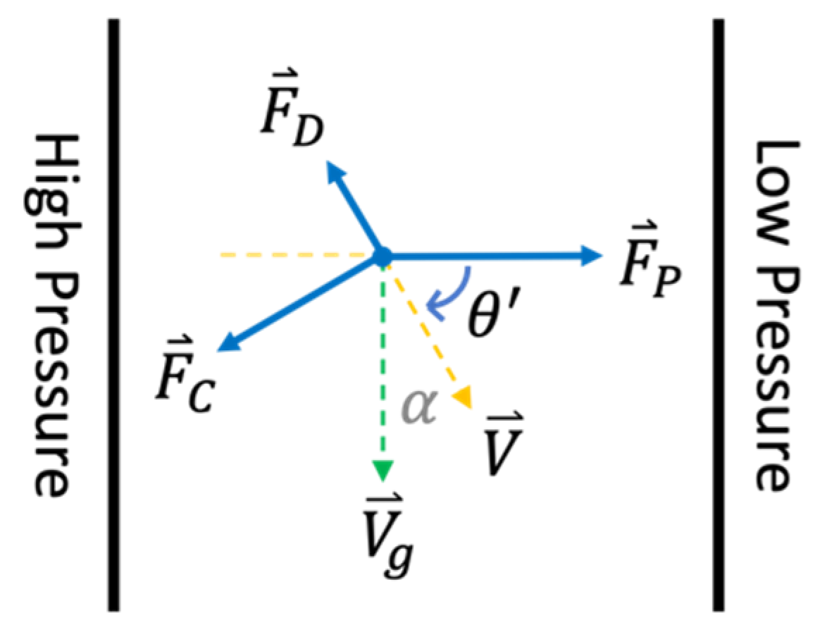
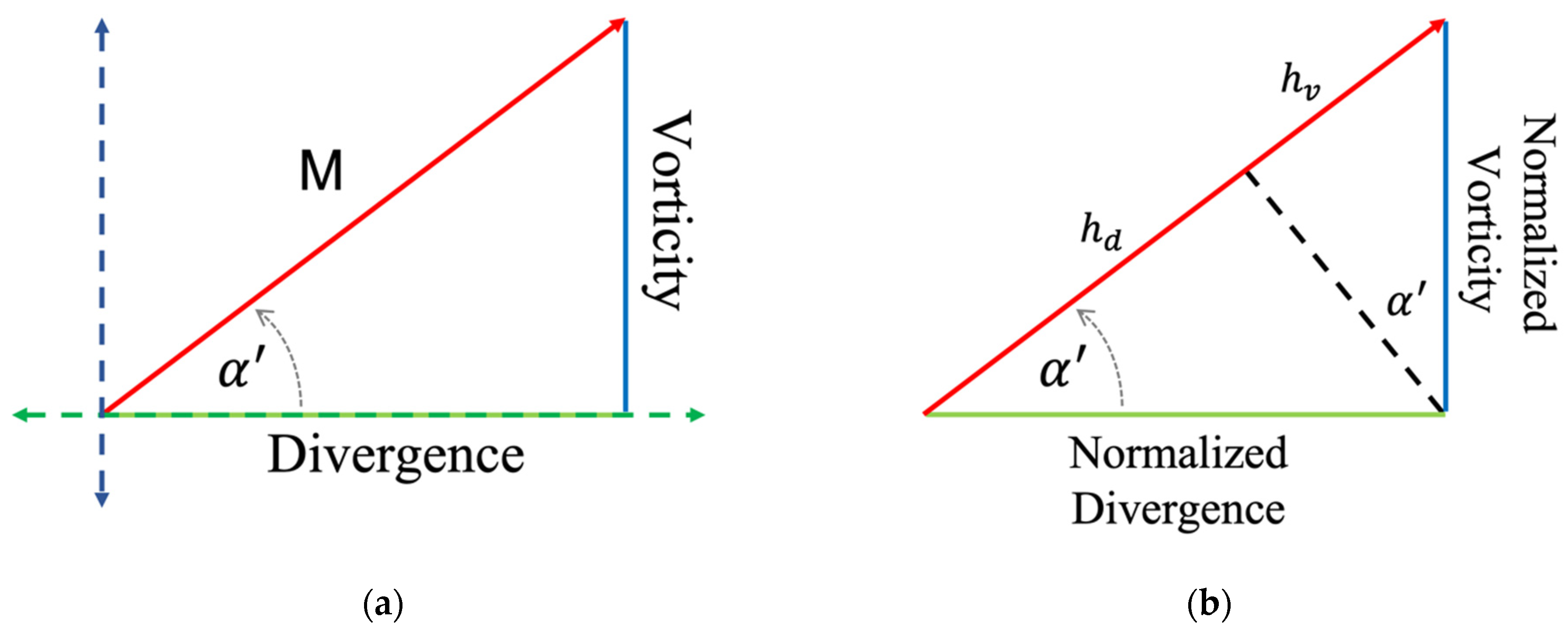
2. Methods
3. Data
4. Results
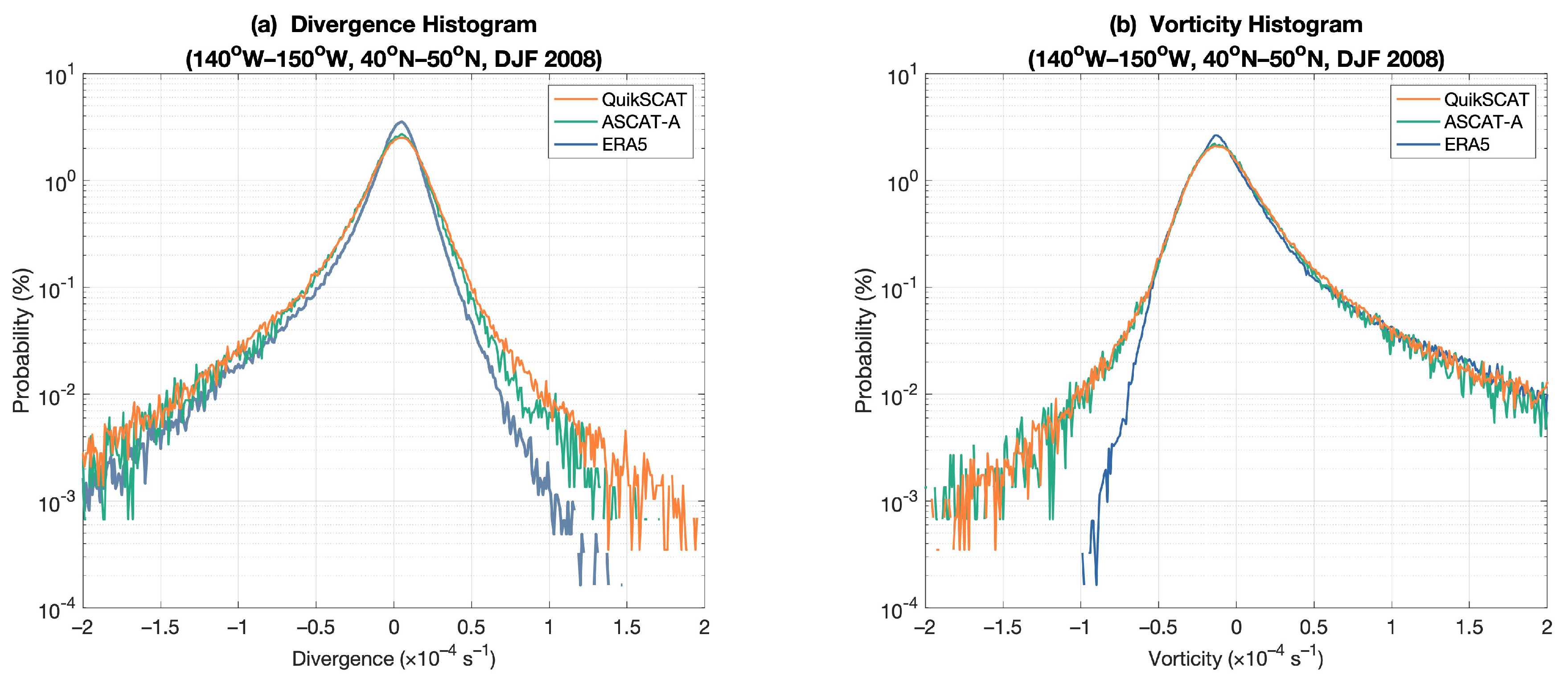
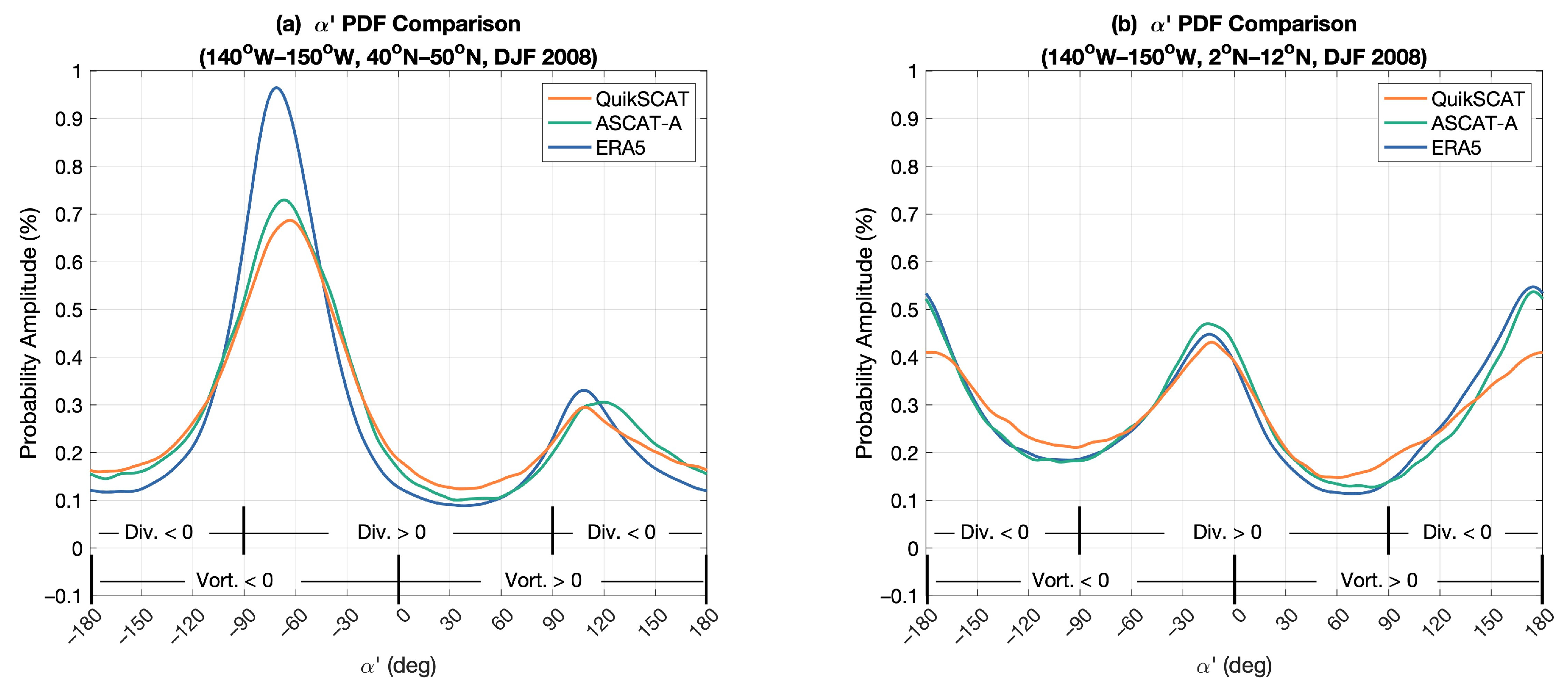
4.1. Divergence and Vorticity Probability Distributions
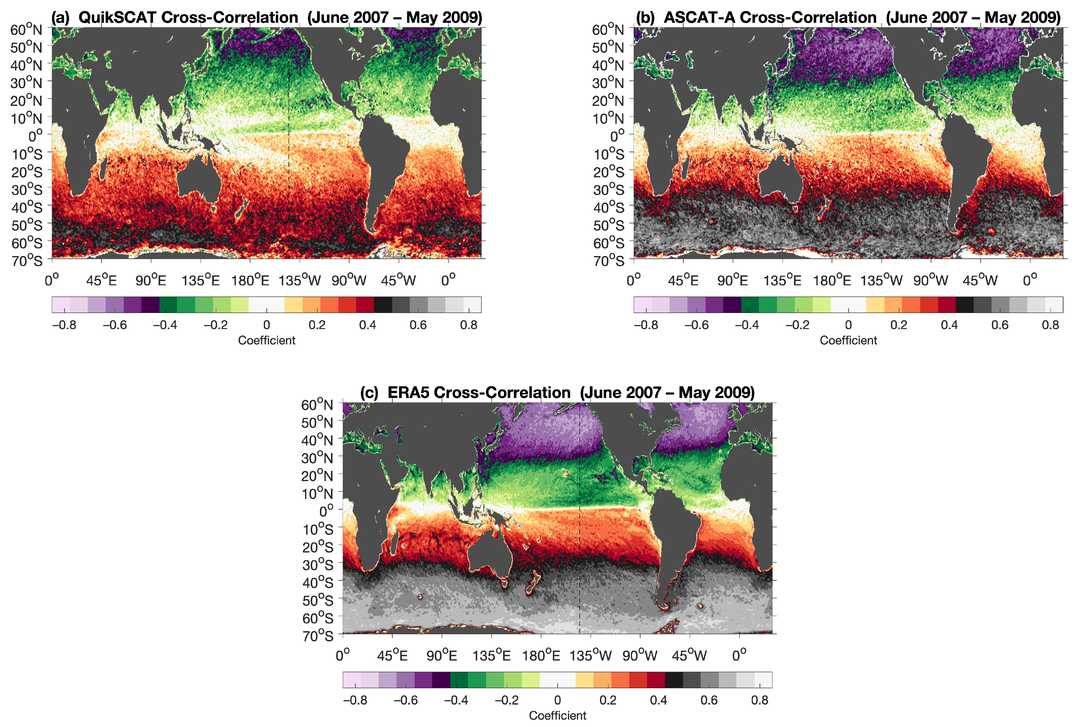
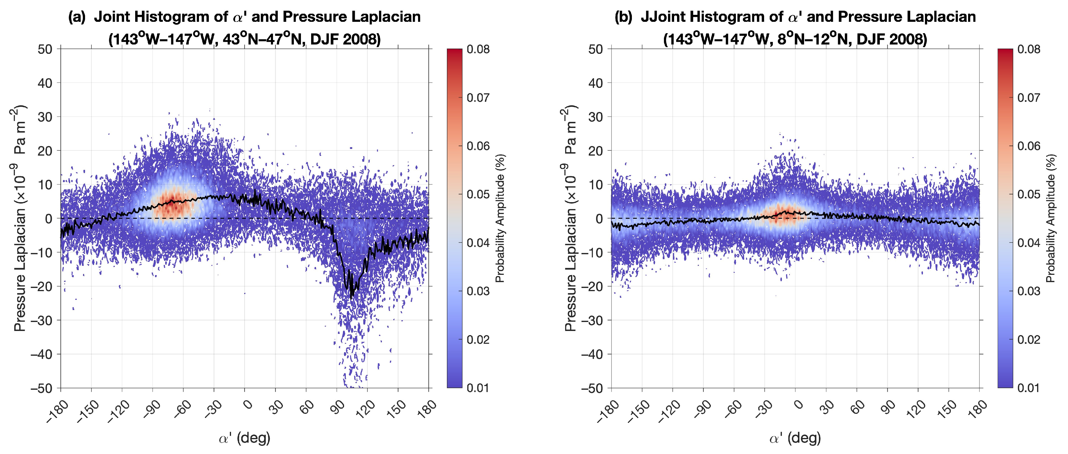
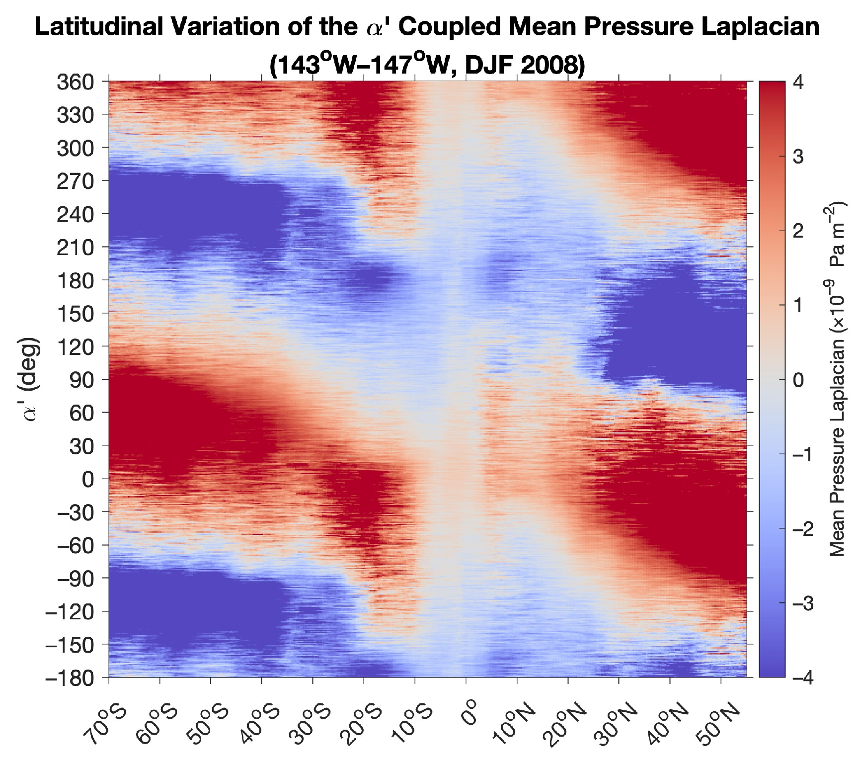
4.2. Correlation of and Pressure
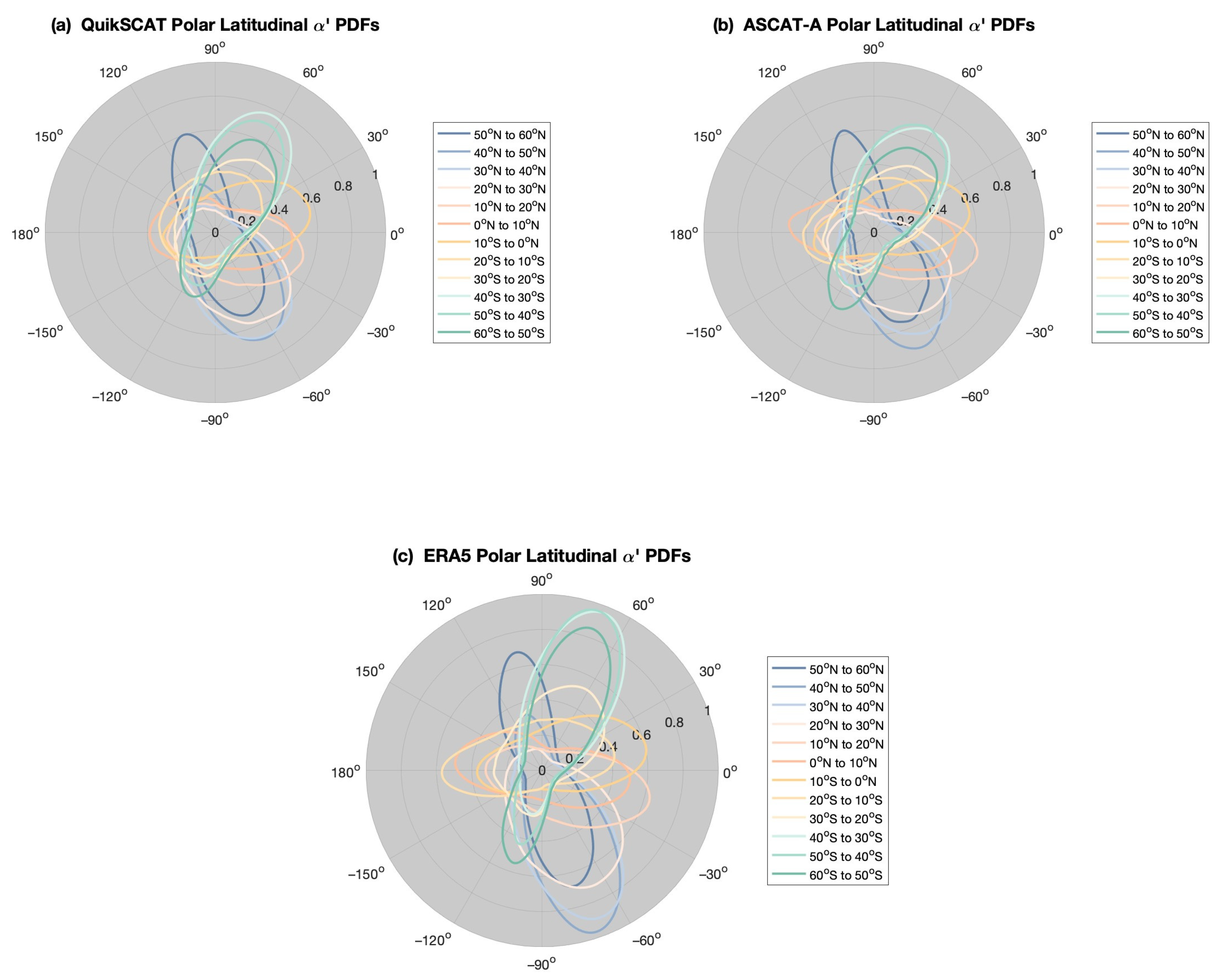
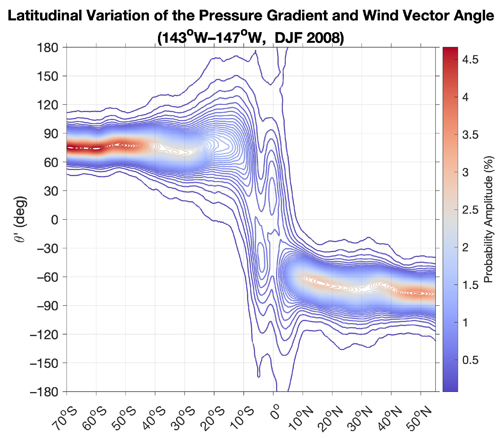
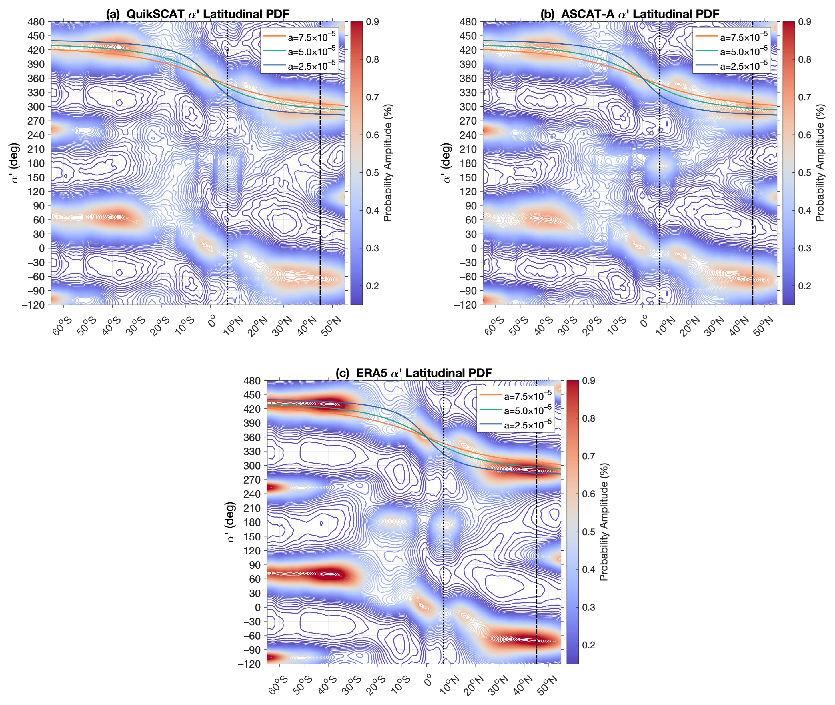
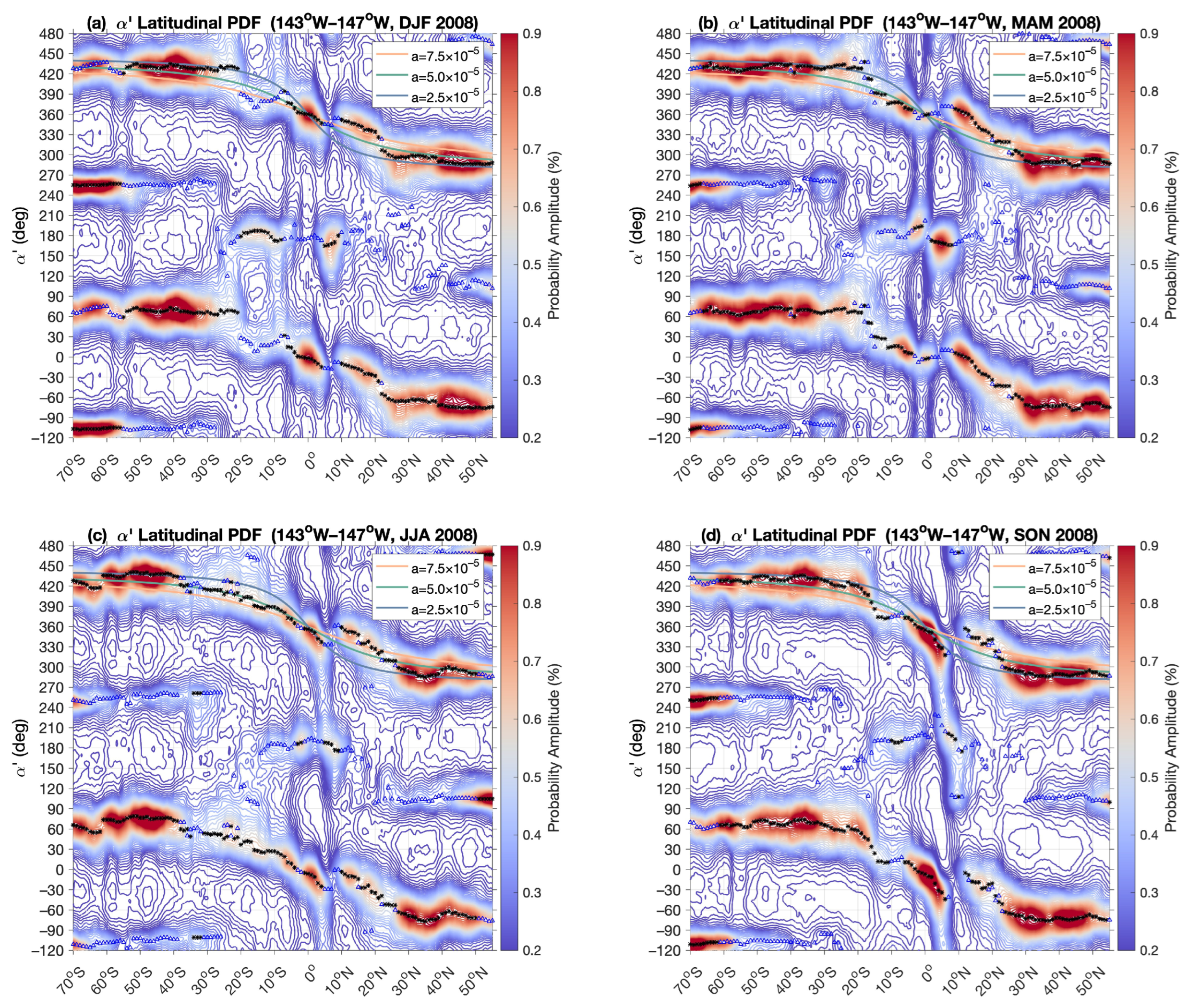
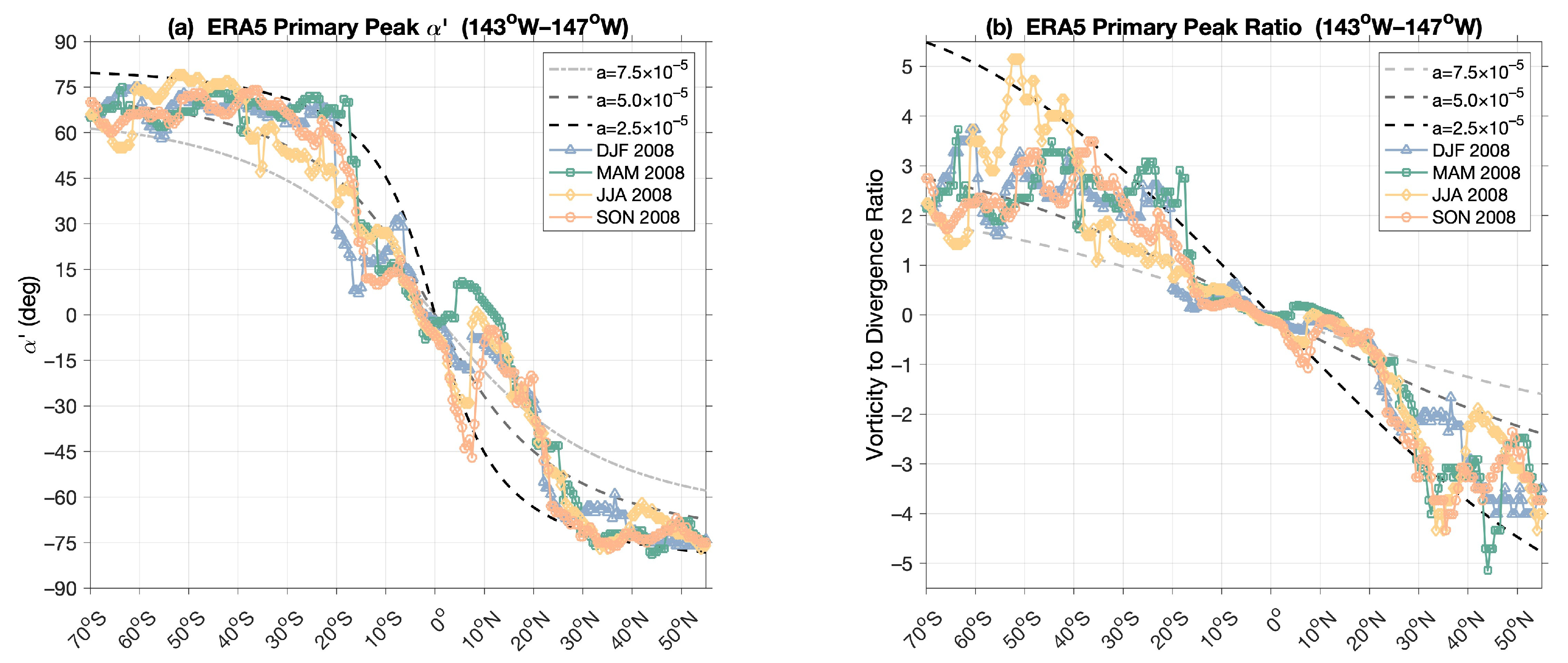
4.3. Latitudinal Probability Distributions
4.4. Seasonal Probability Distributions
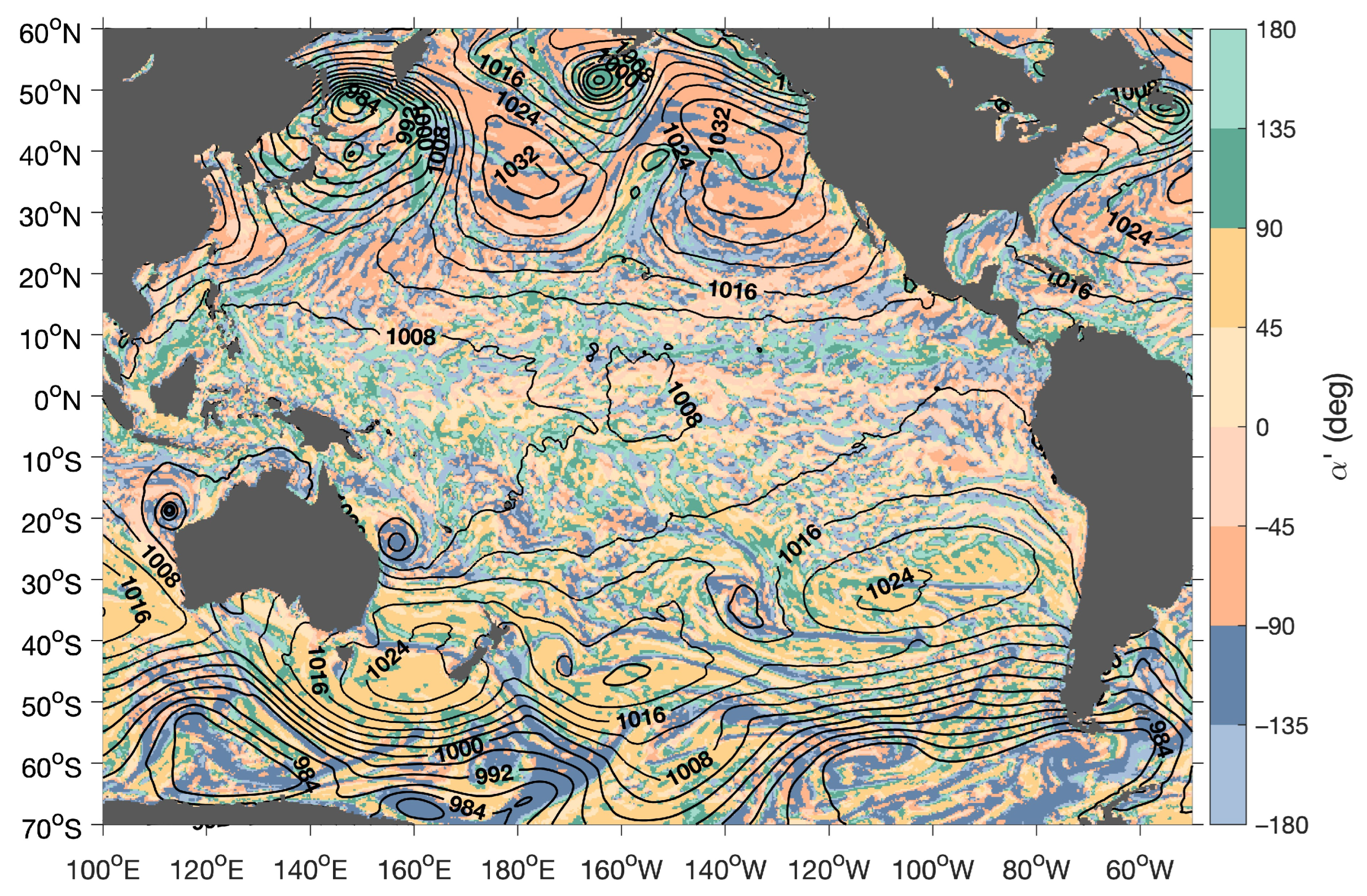
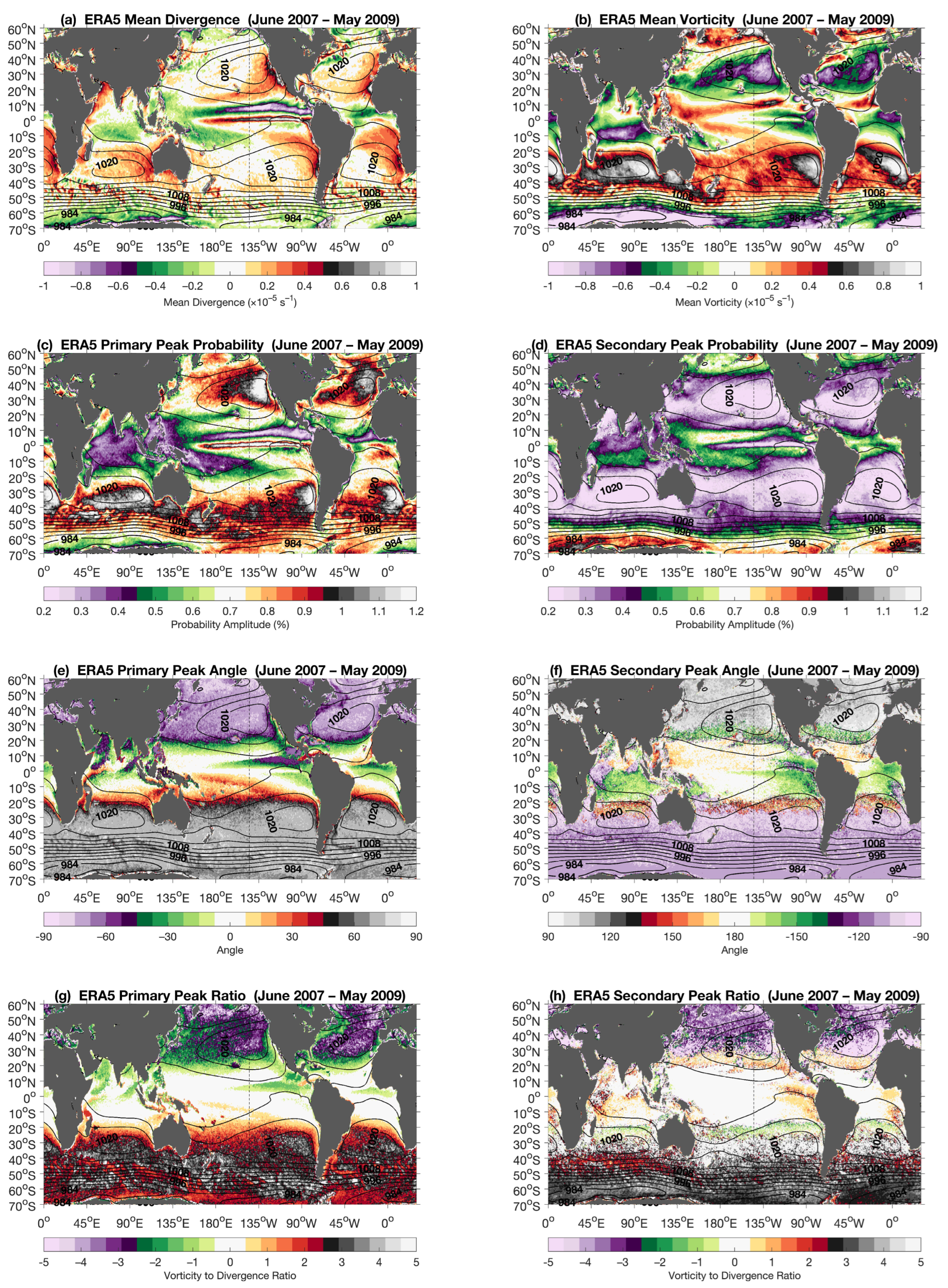
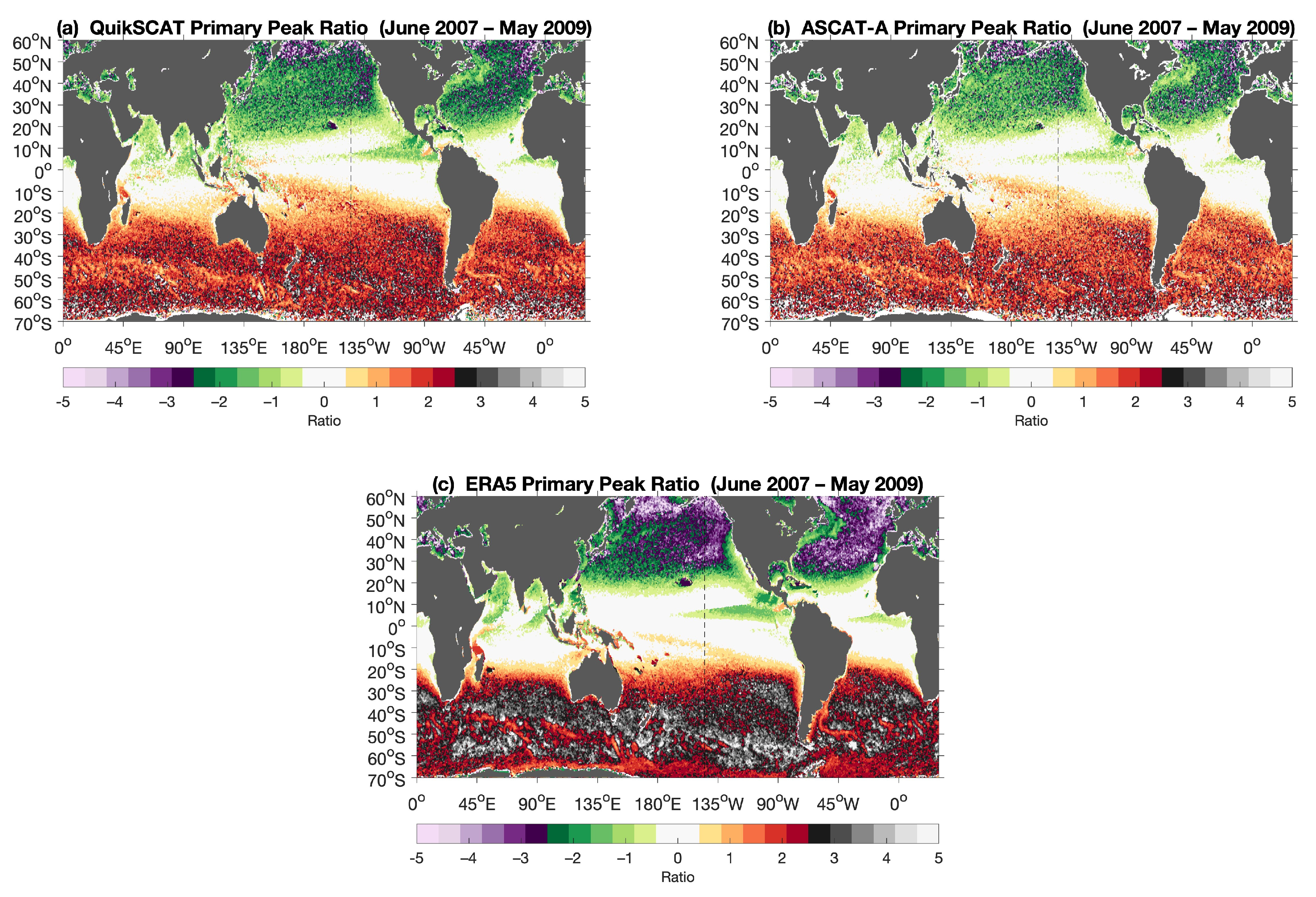
4.5. Global Probability Distributions
5. Discussion
6. Conclusions
Author Contributions
Funding
Data Availability Statement
Conflicts of Interest
References
- Bourassa, M.A.; Meissner, T.; Cerovecki, I.; Chang, P.S.; Dong, X.; De Chiara, G.; Donlon, C.; Dukhovskoy, D.S.; Elya, J.; Fore, A.; et al. Remotely Sensed Winds and Wind Stresses for Marine Forecasting and Ocean Modeling. Front. Mar. Sci. 2019, 6, 443. [Google Scholar] [CrossRef]
- Chelton, D.B.; Schlax, M.G.; Freilich, M.H.; Milliff, R.F. Satellite Measurements Reveal Persistent Small-Scale Features in Ocean Winds. Science 2004, 303, 978–983. [Google Scholar] [CrossRef] [PubMed]
- O’Neill, L.W.; Haack, T.; Durland, T. Estimation of Time-Averaged Surface Divergence and Vorticity from Satellite Ocean Vector Winds. J. Clim. 2015, 28, 7596–7620. [Google Scholar] [CrossRef]
- Milliff, R.F.; Morzel, J.; Chelton, D.B.; Freilich, M.H. Wind Stress Curl and Wind Stress Divergence Biases from Rain Effects on QSCAT Surface Wind Retrievals. J. Atmos. Ocean. Technol. 2004, 21, 1216–1231. [Google Scholar] [CrossRef]
- Bourassa, M.A.; McBeth Ford, K. Uncertainty in Scatterometer-Derived Vorticity. J. Atmos. Ocean. Technol. 2010, 27, 594–603. [Google Scholar] [CrossRef][Green Version]
- Back, L.E.; Bretherton, C.S. On the Relationship between SST Gradients, Boundary Layer Winds, and Convergence over the Tropical Oceans. J. Clim. 2009, 22, 4182–4196. [Google Scholar] [CrossRef]
- Back, L.E.; Bretherton, C.S. A Simple Model of Climatological Rainfall and Vertical Motion Patterns over the Tropical Oceans. J. Clim. 2009, 22, 6477–6497. [Google Scholar] [CrossRef]
- King, G.P.; Portabella, M.; Lin, W.; Stoffelen, A. Correlating Extremes in Wind Divergence with Extremes in Rain over the Tropical Atlantic. Remote Sens. 2022, 14, 1147. [Google Scholar] [CrossRef]
- Vogelzang, J.; Stoffelen, A. ASCAT Ultrahigh-Resolution Wind Products on Optimized Grids. IEEE J. Sel. Top. Appl. Earth Obs. Remote Sens. 2017, 10, 2332–2339. [Google Scholar] [CrossRef]
- Vogelzang, J.; Stoffelen, A. On the Accuracy and Consistency of Quintuple Collocation Analysis of in Situ, Scatterometer, and NWP Winds. Remote Sens. 2022, 14, 4552. [Google Scholar] [CrossRef]
- Wang, Z.; Stoffelen, A.; Zou, J.; Lin, W.; Verhoef, A.; Zhang, Y.; He, Y.; Lin, M. Validation of New Sea Surface Wind Products from Scatterometers Onboard the HY-2B and Metop-C Satellites. IEEE Trans. Geosci. Remote Sens. 2020, 58, 4387–4394. [Google Scholar] [CrossRef]
- Weissman, D.E.; Stiles, B.W.; Hristova-Veleva, S.M.; Long, D.G.; Smith, D.K.; Hilburn, K.A.; Jones, W.L. Challenges to Satellite Sensors of Ocean Winds: Addressing Precipitation Effects. J. Atmos. Ocean. Technol. 2012, 29, 356–374. [Google Scholar] [CrossRef]
- Zhao, K.; Stoffelen, A.; Verspeek, J.; Verhoef, A.; Zhao, C. A Conceptual Rain Effect Model for Ku-Band Scatterometers. IEEE Trans. Geosci. Remote Sens. 2023, 61, 1–9. [Google Scholar] [CrossRef]
- Simpson, I.R.; Bacmeister, J.T.; Sandu, I.; Rodwell, M.J. Why Do Modeled and Observed Surface Wind Stress Climatologies Differ in the Trade Wind Regions? J. Clim. 2018, 31, 491–513. [Google Scholar] [CrossRef]
- Belmonte Rivas, M.; Stoffelen, A. Characterizing Era-Interim and ERA5 Surface Wind Biases Using ASCAT. Ocean Sci. 2019, 15, 831–852. [Google Scholar] [CrossRef]
- Zheng, Q.; Yan, X.-H.; Liu, W.T.; Tang, W.; Kurz, D. Seasonal and Interannual Variability of Atmospheric Convergence Zones in the Tropical Pacific Observed with ERS-1 Scatterometer. Geophys. Res. Lett. 1997, 24, 261–263. [Google Scholar] [CrossRef]
- Žagar, N.; Skok, G.; Tribbia, J. Climatology of the ITCZ Derived from ERA Interim Reanalyses. J. Geophys. Res. 2011, 116, D15. [Google Scholar] [CrossRef]
- Grodsky, S.A.; Carton, J.A. The Intertropical Convergence Zone in the South Atlantic and the Equatorial Cold Tongue. J. Clim. 2003, 16, 723–733. [Google Scholar] [CrossRef]
- Liu, W.T.; Xie, X. Double Intertropical Convergence Zones-a New Look Using Scatterometer. Geophys. Res. Lett. 2002, 29, 29-1–29-4. [Google Scholar] [CrossRef]
- Meenu, S.; Rajeev, K.; Parameswaran, K.; Suresh Raju, C. Characteristics of the Double Intertropical Convergence Zone over the Tropical Indian Ocean. J. Geophys. Res. 2007, 112, D11. [Google Scholar] [CrossRef]
- Halpern, D.; Hung, C.-W. Satellite Observations of the Southeast Pacific Intertropical Convergence Zone during 1993–1998. J. Geophys. Res. Atmos. 2001, 106, 28107–28112. [Google Scholar] [CrossRef]
- Luis, A.J.; Pandey, P.C. Characteristics of Atmospheric Divergence and Convergence in the Indian Ocean Inferred from Scatterometer Winds. Remote Sens. Environ. 2005, 97, 231–237. [Google Scholar] [CrossRef]
- Milliff, R.F.; Morzel, J. The Global Distribution of the Time-Average Wind Stress Curl from NSCAT. J. Atmos. Sci. 2001, 58, 109–131. [Google Scholar] [CrossRef]
- O’Neill, L.W.; Chelton, D.B.; Esbensen, S.K. The Effects of SST-Induced Surface Wind Speed and Direction Gradients on Midlatitude Surface Vorticity and Divergence. J. Clim. 2010, 23, 255–281. [Google Scholar] [CrossRef]
- O’Neill, L.W.; Haack, T.; Chelton, D.B.; Skyllingstad, E. The Gulf Stream Convergence Zone in the Time-Mean Winds. J. Atmos. Sci. 2017, 74, 2383–2412. [Google Scholar] [CrossRef]
- Holbach, H.M.; Bourassa, M.A. The Effects of Gap-Wind-Induced Vorticity, the Monsoon Trough, and the ITCZ on East Pacific Tropical Cyclogenesis. Mon. Weather. Rev. 2014, 142, 1312–1325. [Google Scholar] [CrossRef]
- King, G.P.; Vogelzang, J.; Stoffelen, A. Upscale and Downscale Energy Transfer over the Tropical Pacific Revealed by Scatterometer Winds. J. Geophys. Res. Ocean. 2015, 120, 346–361. [Google Scholar] [CrossRef]
- Masunaga, R.; Nakamura, H.; Taguchi, B.; Miyasaka, T. Processes Shaping the Frontal-Scale Time-Mean Surface Wind Convergence Patterns around the Gulf Stream and Agulhas Return Current in Winter. J. Clim. 2020, 33, 9083–9101. [Google Scholar] [CrossRef]
- Wentz, F.J.; Ricciardulli, L.; Rodriguez, E.; Stiles, B.W.; Bourassa, M.A.; Long, D.G.; Hoffman, R.N.; Stoffelen, A.; Verhoef, A.; O’Neill, L.W.; et al. Evaluating and Extending the Ocean Wind Climate Data Record. IEEE J. Sel. Top. Appl. Earth Obs. Remote Sens. 2017, 10, 2165–2185. [Google Scholar] [CrossRef]
- Holton, J.R. An Introduction to Dynamic Meteorology; Elsevier Academic Press: Amsterdam, The Netherlands, 2009. [Google Scholar]
- Jacox, M.G.; Edwards, C.A.; Hazen, E.L.; Bograd, S.J. Coastal Upwelling Revisited: Ekman, Bakun, and Improved Upwelling Indices for the U.S. West Coast. J. Geophys. Res. Ocean. 2018, 123, 7332–7350. [Google Scholar] [CrossRef]
- Patoux, J.; Brown, R.A. Spectral Analysis of QuikSCAT Surface Winds and Two-Dimensional Turbulence. J. Geophys. Res. Atmos. 2001, 106, 23995–24005. [Google Scholar] [CrossRef]
- Nicholls, S.; Leighton, J. An Observational Study of the Structure of Stratiform Cloud Sheets: Part I. Structure. Q. J. R. Meteorol. Soc. 1986, 112, 431–460. [Google Scholar] [CrossRef]
- Wood, R. Stratocumulus Clouds. Mon. Weather Rev. 2012, 140, 2373–2423. [Google Scholar] [CrossRef]
- Lounesto, P. Clifford Algebras and Spinors, 2nd ed.; London Mathematical Society Lecture Note Series; Cambridge University Press: Cambridge, UK, 2001. [Google Scholar] [CrossRef]
- Chelton, D.B.; Esbensen, S.K.; Schlax, M.G.; Thum, N.; Freilich, M.H.; Wentz, F.J.; Gentemann, C.L.; McPhaden, M.J.; Schopf, P.S. Observations of Coupling between Surface Wind Stress and Sea Surface Temperature in the Eastern Tropical Pacific. J. Clim. 2001, 14, 1479–1498. [Google Scholar] [CrossRef]
- Hashizume, H.; Xie, S.-P.; Fujiwara, M.; Shiotani, M.; Watanabe, T.; Tanimoto, Y.; Liu, W.T.; Takeuchi, K. Direct Observations of Atmospheric Boundary Layer Response to SST Variations Associated with Tropical Instability Waves over the Eastern Equatorial Pacific. J. Clim. 2002, 15, 3379–3393. [Google Scholar] [CrossRef]
- Pezzi, L.P.; Souza, R.B.; Farias, P.C.; Acevedo, O.; Miller, A.J. Air-Sea Interaction at the Southern Brazilian Continental Shelf: In Situ Observations. J. Geophys. Res. Ocean. 2016, 121, 6671–6695. [Google Scholar] [CrossRef]
- Hennemuth, B.; Lammert, A. Determination of the Atmospheric Boundary Layer Height from Radiosonde and Lidar Backscatter. Bound. Layer Meteorol. 2006, 120, 181–200. [Google Scholar] [CrossRef]
- SeaPAC. QuikSCAT Level 2B Ocean Wind Vectors in 12.5km Slice Composites Version 4.1. Ver. 4.1. PO.DAAC, CA, USA. 2020. Available online: https://podaac.jpl.nasa.gov/dataset/QSCAT_LEVEL_2B_OWV_COMP_12_KUSST_LCRES_4.1 (accessed on 20 August 2021).
- EUMETSAT/OSI SAF. MetOp-A ASCAT Level 2 25.0 km Ocean Surface Wind Vectors. Ver. Operational/Near-Real-Time. PO.DAAC, CA, USA. 2010. Available online: https://podaac.jpl.nasa.gov/dataset/ASCATA-L2-25km (accessed on 22 January 2022).
- Copernicus Climate Change Service (C3S) (2017): ERA5: Fifth Generation of ECMWF Atmospheric Reanalyses of the Global Climate. Copernicus Climate Change Service Climate Data Store (CDS). Available online: https://cds.climate.copernicus.eu/cdsapp#!/home (accessed on 3 March 2019).
- Hersbach, H.; Bell, B.; Berrisford, P.; Hirahara, S.; Horányi, A.; Muñoz-Sabater, J.; Nicolas, J.; Peubey, C.; Radu, R.; Schepers, D.; et al. The ERA5 Global Reanalysis. Q. J. R. Meteorol. Soc. 2020, 146, 1999–2049. [Google Scholar] [CrossRef]
- Cleveland, W.S.; Devlin, S.J. Locally Weighted Regression: An Approach to Regression Analysis by Local Fitting. J. Am. Stat. Assoc. 1988, 83, 596–610. [Google Scholar] [CrossRef]
- Schlax, M.G.; Chelton, D.B. Frequency Domain Diagnostics for Linear Smoothers. J. Am. Stat. Assoc. 1992, 87, 1070–1081. [Google Scholar] [CrossRef]
- de Kloe, J.; Stoffelen, A.; Verhoef, A. Improved Use of Scatterometer Measurements by Using Stress-Equivalent Reference Winds. IEEE J. Sel. Top. Appl. Earth Obs. Remote Sens. 2017, 10, 2340–2347. [Google Scholar] [CrossRef]
- Liu, W.T.; Tang, W. Equivalent Neutral Wind (NASA Technical Report); Jet Propulsion Lab., California Inst. Of Tech.: Pasadena, CA, USA, 1996; No. NASA-CR-203424. [Google Scholar]
- Ross, D.M.; Overland, J.E.; Plerson, W.J.; Cardone, V.J.; McPherson, R.J.; Yu, T.-W. Chapter 4 Oceanic Surface Winds. Adv. Geophys. 1985, 27, 101–140. [Google Scholar] [CrossRef]
- Parfitt, R.; Seo, H. A New Framework for Near-Surface Wind Convergence over the Kuroshio Extension and Gulf Stream in Wintertime: The Role of Atmospheric Fronts. Geophys. Res. Lett. 2018, 45, 9909–9918. [Google Scholar] [CrossRef]
- Small, R.J.; de Szoeke, S.P.; Xie, S.; Luke; Seo, H.; Song, Q.Q.; Cornillon, P.; Spall, M.; Minobe, S. Air–Sea Interaction over Ocean Fronts and Eddies. Dyn. Atmos. Ocean. 2008, 45, 274–319. [Google Scholar] [CrossRef]
- Seo, H.; O’Neill, L.W.; Bourassa, M.A.; Czaja, A.; Drushka, K.; Edson, J.B.; Fox-Kemper, B.; Frenger, I.; Gille, S.T.; Kirtman, B.; et al. Ocean Mesoscale and Frontal-Scale Ocean–Atmosphere Interactions and Influence on Large-Scale Climate: A Review. J. Clim. 2023, 36, 1981–2013. [Google Scholar] [CrossRef]
- Small, R.J.; Rousseau, V.; Parfitt, R.L.; Laurindo, L.C.; O’Neill, L.W.; Masunaga, R.; Schneider, N.; Chang, P.S. Near-Surface Wind Convergence over the Gulf Stream—The Role of SST Revisited. J. Clim. 2023, 36, 5527–5548. [Google Scholar] [CrossRef]
- Minobe, S.; Kuwano-Yoshida, A.; Komori, N.; Xie, S.-P.; Small, R.J. Influence of the Gulf Stream on the Troposphere. Nature 2008, 452, 206–209. [Google Scholar] [CrossRef]


Disclaimer/Publisher’s Note: The statements, opinions and data contained in all publications are solely those of the individual author(s) and contributor(s) and not of MDPI and/or the editor(s). MDPI and/or the editor(s) disclaim responsibility for any injury to people or property resulting from any ideas, methods, instructions or products referred to in the content. |
© 2024 by the authors. Licensee MDPI, Basel, Switzerland. This article is an open access article distributed under the terms and conditions of the Creative Commons Attribution (CC BY) license (https://creativecommons.org/licenses/by/4.0/).
Share and Cite
Jacobs, R.; O’Neill, L.W. Co-Variability between the Surface Wind Divergence and Vorticity over the Ocean. Remote Sens. 2024, 16, 451. https://doi.org/10.3390/rs16030451
Jacobs R, O’Neill LW. Co-Variability between the Surface Wind Divergence and Vorticity over the Ocean. Remote Sensing. 2024; 16(3):451. https://doi.org/10.3390/rs16030451
Chicago/Turabian StyleJacobs, Robert, and Larry W. O’Neill. 2024. "Co-Variability between the Surface Wind Divergence and Vorticity over the Ocean" Remote Sensing 16, no. 3: 451. https://doi.org/10.3390/rs16030451
APA StyleJacobs, R., & O’Neill, L. W. (2024). Co-Variability between the Surface Wind Divergence and Vorticity over the Ocean. Remote Sensing, 16(3), 451. https://doi.org/10.3390/rs16030451