Optical Frequency Sweeping Nonlinearity Measurement Based on a Calibration-free MZI

Abstract

Frequency sweeping linearity is essential for Frequency-Modulated Continuous Wave (FMCW) Light Detection and Ranging (LIDAR), as it impacts the ranging resolution and accuracy of the system. Pre-distortion methods can correct for frequency sweeping nonlinearity; however, residual minor nonlinearities can still degrade the system ranging resolution, especially at far distances. Therefore, the precise measurement of minor nonlinearities is particularly essential for long-range FMCW LIDAR. This paper proposes a calibration-free MZI for measuring optical frequency sweeping nonlinearity, which involves alternately inserting two short polarization-maintaining fibers with different delays into one arm of an MZI, and after two rounds of beat collection, the optical frequency sweep curve of the light source is accurately measured for nonlinearity evaluation. Using the proposed method, the nonlinearity of a frequency-swept laser source is measured to be 0.2113%, and the relative nonlinearity is 5.3560 × 10⁻⁵. With the measured frequency sweep curve, we simulate the beat signal and compare it with the collected beat signal in time and frequency domain, to verify the accuracy of the proposed method. A test conducted at 24.1 °C, 30.4 °C, 39.5 °C and 44.0 °C demonstrate the method’s insensitivity to temperature fluctuations. Based on the proposed MZI, a tunable laser is pre-distorted and then used as light source of a FMCW lidar. A wall at 45 m and a building at 1.2 km are ranged by the lidar respectively. Before and after laser pre-distortion, the FWHM of echo beat spectrum are 25.635 kHz and 9.736 kHz for 45 m, 747.880 kHz and 22.012 kHz for 1.2 km.

1. Introduction

With the continuous advancement of technology and the robust growth of the industrial manufacturing sector, there has been an increasing demand for higher precision and accuracy in absolute distance measurement. Laser radar, or LIDAR, which stands for Light Detection and Ranging, has emerged as a prominent technique due to its non-contact and high-resolution ranging capabilities. To date, LIDAR has been widely applied in various fields, including remote sensing, wind speed measurement, environmental monitoring, and autonomous driving [1,2,3,4]. The existing LIDAR ranging mechanisms are primarily categorized into incoherent and coherent measurement methods. Incoherent measurement methods are essentially based on the detection of changes in reflected light intensity, and due to their direct and straightforward detection approach, they are extensively used in the automotive industry [4]. However, this incoherent measurement mechanism is susceptible to interference from ambient stray light, which compromises its stability. On the other hand, coherent measurement techniques are fundamentally based on the frequency demodulation of optical interference beat signals [5]. The current mainstream coherent LIDAR is the Frequency-Modulated Continuous Wave (FMCW) LIDAR, which offers advantages such as resistance to environmental light interference, high measurement resolution, and high precision [6]. FMCW LIDAR modulates the frequency of the emitted light and employs coherent detection at the receiver end. The target echo light is mixed with a local oscillator light, which is a copy of transmitted light, and the round-trip distance information is converted into a beat signal [7]. FMCW LIDAR plays a significant role in the field of precision measurement [8,9]. Furthermore, FMCW LIDAR is capable of simultaneously demodulating velocity and distance in a single measurement, making it a research focus in the field of absolute range measurement in recent years [10].

In practical applications, due to the nonlinear relationship between the injected current and the frequency modulation response of a semiconductor laser, as well as the impact of the external environment, the optical frequency sweep signal output by a FMCW LIDAR light source is not completely linearized [11]. The nonlinearity will broaden the spectrum of a beat signal at the receiving end, which affects the resolution of two close-range targets and ultimately leads to the system ranging resolution degradation [12]. It has been reported that the spectrum broadening of a beat signal caused by optical frequency sweeping nonlinearity will increase with target distance. For smaller optical frequency sweep nonlinearities, FMCW LIDAR has a higher tolerance at a close range, but at a long range (such as kilometers), a smaller optical frequency sweeping nonlinearity will also cause obvious spectrum broadening [13].

To address such issues, a variety of optical frequency sweep linearization methods have been proposed to suppress the optical frequency sweeping nonlinearity of a light source, including equispaced-phase resampling, iterative algorithm, and photoelectric phase-locked loop [14,15,16]. In these studies, the accurate measurement of the optical frequency sweeping nonlinearity of a light source is an indispensable part. In recent years, the measurement of the frequency sweeping nonlinearity of an FMCW LIDAR light source has mostly been conducted based on a Mach–Zehnder interferometer [17,18]. In an experimental research using a fiber MZI, accurate control of the optical path difference between the two arms of an MZI is crucial, which is fatal for the accuracy of nonlinearity measurement. Consequently, it is required to calibrate the arm length difference of a fiber MZI in advance. Currently, the primary methods for calibrating the arm length difference involve either direct calibration or indirect calibration through the measurement of the lengths of the fibers utilized in constructing the MZI. However, these methodologies possess significant limitations.

The reported methods for directly calibrating the arm length difference of a fiber MZI mainly include current modulation of the light source and observation of interference fringes, interferometer interference spectrum measurement, white light interferometry, and optical reflectometry [19,20,21]. These methods, despite their conceptual simplicity, are cumbersome in operation and rely heavily on manual procedures, necessitating visual assessment by the human eye, which not only introduces subjectivity but also limits the measurement range. Consequently, these constraints impede their widespread adoption in practical applications. Furthermore, these techniques often require auxiliary interferometers, spectrometers, or other specialized equipment, with equipment configurations that are typically fixed, thereby lacking the flexibility needed to adapt to diverse scenarios. This inflexibility further complicates their implementation in real-world settings, exacerbating the challenges associated with their broader use.

The reported methods for indirectly calibrating the arm length difference of a fiber MZI by measuring the lengths of the fibers include Optical Time Domain Reflectometry (OTDR), Optical Frequency Domain Reflectometry (OFDR), and Optical Correlation Domain Reflectometry (OCDR) [22,23,24,25]. While these methodologies offer precise measurements of the arm length difference, they still present some issues. In practical scenarios, especially over extended periods (>1 s), the primary factor causing variations in fiber length is thermal effect [26]. This means that the arm length difference is susceptible to fluctuations in the ambient temperature of the experimental environment. Such temperature-induced changes can lead to significant discrepancies in the measurement of the optical frequency sweep, thereby affecting the accuracy of the system. The thermal sensitivity of these measurements poses a significant challenge for the reliable operation of an MZI in applications where environmental conditions cannot be tightly controlled.

In this paper, we propose an optical frequency sweeping nonlinearity measurement based on a calibration-free MZI. It does not need to calibrate the optical path difference between the two arms of an MZI in advance. Two short polarization-maintaining fibers with different lengths (time delays already known) are inserted to one arm of an MZI alternatively. By calculating the phase of two beats, the optical frequency sweep curve of the light source can be measured, and then its nonlinearity can be evaluated. When the experimental setup needs to be relocated, only the two alternative fibers with known delays need to be carried, which implies that this method possesses a high degree of flexibility. Moreover, the accuracy of the measurement is less susceptible to environmental temperature fluctuations, which makes it applicable for the frequency sweep linearization of the FMCW LIDAR light source, as well as for studies related to range and velocity measurement and three-dimensional imaging [8,12].

2. Principle

The schematic diagram of a calibration-free MZI for measuring the optical frequency sweeping nonlinearity is illustrated in Figure 1. The MZI’s function is to down-convert the optical frequency emitted by a laser to an intermediate frequency, enabling the reconstruction of the laser’s optical frequency sweep curve from the beat signal. With the modulation of a triangular wave, the tunable laser emits an optical frequency sweep signal $v_s\left(t\right)$ that is split into two channels, labeled as a and b, in the MZI. Channel-a serves as the reference optical signal $v_r\left(t\right)$, while channel-b serves as the delayed optical signal $v_d\left(t\right)$. A segment of a fiber on channel-b is replaced by two fibers with different lengths or delays, which are accurately pre-measured. The beat signal ${\varphi }_b\left(t\right)$ resulting from the mixing of the optical signals on channels-a and -b is received by a balanced photodetector (BPD) and subsequently sampled by an oscilloscope (OSC). A personal computer (PC) reads the signals from the oscilloscope and processes it using a Hilbert transform (HT) to derive an optical frequency sweep curve output by the laser.

The phase of the beat signal ${\varphi }_b\left(t\right)$ can be obtained by applying an HT to the beat signal [27]. The delay difference between the two arms of the MZI is denoted as $\tau$. when $\tau$ is extremely small, ${\varphi }_b\left(t\right)$ can be approximated as [28]

$${\varphi }_b\left(t\right)=2\pi v_s\left(t\right)\tau$$

(1)

where $v_s\left(t\right)$ is the optical frequency sweep signal output by the tunable laser.

When the alternative fiber b1 is inserted into channel-b of the MZI, the total delay difference between the two arms of the interferometer is ${\tau }_{b1\_total}$; when b2 is inserted, the total delay difference is ${\tau }_{b2\_total}$. Then after two measurements through the MZI with different arm delays, the beat phases can be respectively obtained as

$${\varphi }_{b1}\left(t\right)=2\pi v_s\left(t\right){\tau }_{b1\_total}$$

(2)

$${\varphi }_{b2}\left(t\right)=2\pi v_s\left(t\right){\tau }_{b2\_total}$$

(3)

where ${\varphi }_{b1}\left(t\right)$ and ${\varphi }_{b2}\left(t\right)$ are the beat phases obtained when the alternative fibers b1 and b2 are respectively inserted into channel-b of the MZI. The prerequisite for the validity of Equations (2) and (3) is that the repeatability of the optical frequency-modulated curve output by the laser is good enough in a short time; i.e., $v_s\left(t\right)$ does not significantly change with time or remains stable over a short period. By subtracting the beat phases obtained from the two measurements, denoting $\Delta \tau ={\tau }_{b1\_total}-{\tau }_{b2\_total}$, $\Delta \varphi \left(t\right)={\varphi }_{b1}\left(t\right)-{\varphi }_{b2}\left(t\right)$, we can obtain

$$\Delta \varphi \left(t\right)=2\pi v_s\left(t\right)·\Delta \tau$$

(4)

where $\Delta \varphi \left(t\right)$ is the difference between the phases ${\varphi }_{b1}\left(t\right)$ and ${\varphi }_{b2}\left(t\right)$, and $\Delta \tau$ is the difference between the total delay differences ${\tau }_{b1\_total}$ and ${\tau }_{b2\_total}$. Note that the total delay difference between the two arms of the MZI in Equations (2) and (3), i.e., ${\tau }_{b1\_total}$ and ${\tau }_{b2\_total}$, should include the delays caused by the alternative fibers, i.e., ${\tau }_{b1}$ and ${\tau }_{b2}$ (known), and the delay difference ${\tau }_{other}$ caused by the other optical fibers connecting the optical devices, that is, ${\tau }_{b1\_total}={\tau }_{b1}+{\tau }_{other}$, ${\tau }_{b2\_total}={\tau }_{b2}+{\tau }_{other}$, then $\Delta \tau ={\tau }_{b1}-{\tau }_{b2}$. In this way, $v_s\left(t\right)$ can be written as

$$v_s\left(t\right)={\displaystyle \frac{\Delta \varphi \left(t\right)}{2\pi ({\tau }_{b1}-{\tau }_{b2})}}$$

(5)

It can be seen here that $\Delta \tau$ is obtained by the difference between the known delays, ${\tau }_{b1}$ and ${\tau }_{b2}$, of the alternative fibers, and we do not calibrate the optical path difference or delay difference between the two arms of the MZI. Compared with the reported methods, when the delays ${\tau }_{b1}$ and ${\tau }_{b2}$ of the two alternative fibers with different lengths are known, $v_s\left(t\right)$ can be calculated by two beat measurements in this paper, without calibrating the total arm length difference of the MZI. This method requires only that the delays ${\tau }_{b1}$ and ${\tau }_{b2}$ are known quantities, with no specific demands on other configurations of the interferometer, thus providing high flexibility to accommodate various measurement scenarios. Additionally, the two alternative fibers are kept in a room-temperature environment and are alternately inserted into the MZI for experimental measurements. Despite the fact that the lengths or delays of the fibers connecting other optical components may be subject to changes due to temperature fluctuations during the course of the experiment, they are not involved in the calculation of the optical frequency sweep curve $v_s\left(t\right)$. That is to say, fluctuations of the experimental ambient temperature have very little effect on the measurement of the optical frequency sweep in this paper, which further ensures the accuracy of the measured optical frequency sweep curve $v_s\left(t\right)$.

3. Experiments

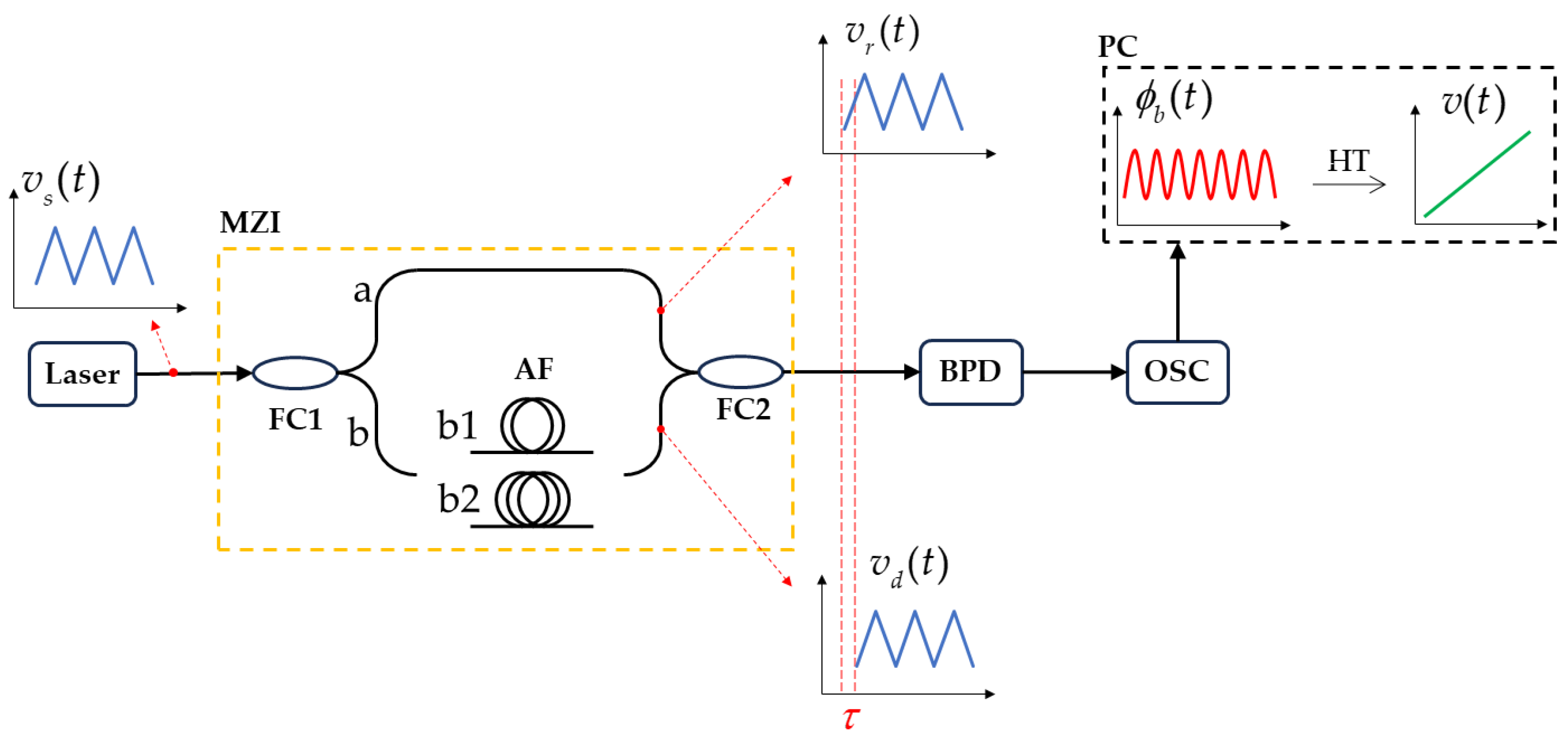
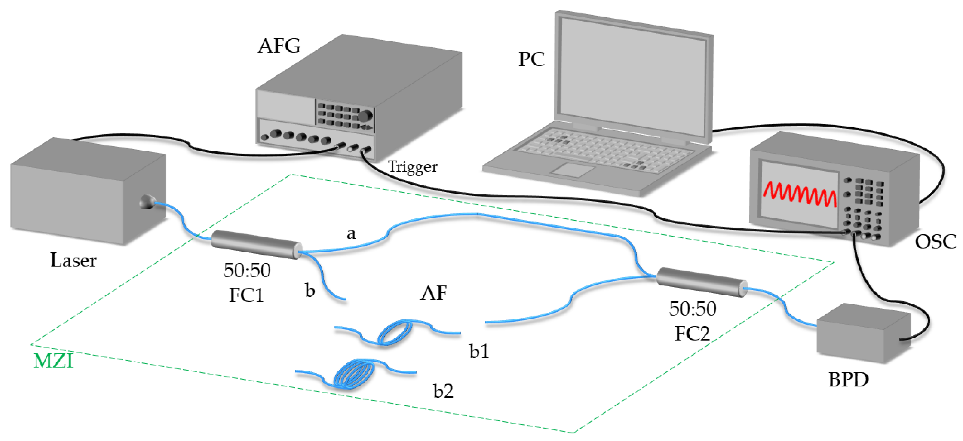
The experimental setup used in the optical frequency sweep nonlinear measurement experiment is depicted in Figure 2. In the experiment, the tunable laser is an ultra-narrow linewidth laser module of 1550 nm, and the frequency modulation factor is about 54 MHz/V. The arbitrary function generator (AFG) generates a modulated triangular wave to modulate the laser. The frequency sweep light output by the laser is split by a $1\times 2$ fiber coupler (FC1) with a coupling ratio of 50:50. The length and delay information of the alternative fiber (AF) in channel-b are shown in

Table 1. The length and delay information of the AF in channel-b of the MZI.

Alternative Fiber	Length (m)	Delay (ns)
b1	2.02322	9.90039 (${\tau }_{b1}$)
b2	5.01827	24.55631 (${\tau }_{b2}$)

. The reference optical signal and the delayed optical signal are mixed at a 3 dB fiber coupler (FC2) to form a beat signal, which is then received by the balanced photodetector (BPD) and finally displayed on the oscilloscope (OSC). A personal computer (PC) is connected to the oscilloscope, which reads the data from the oscilloscope. The PC then performs a Hilbert transform (HT) on the beat signal to extract the optical frequency sweep signal and calculate its nonlinearity.

3.1. The Repeatability Measurement

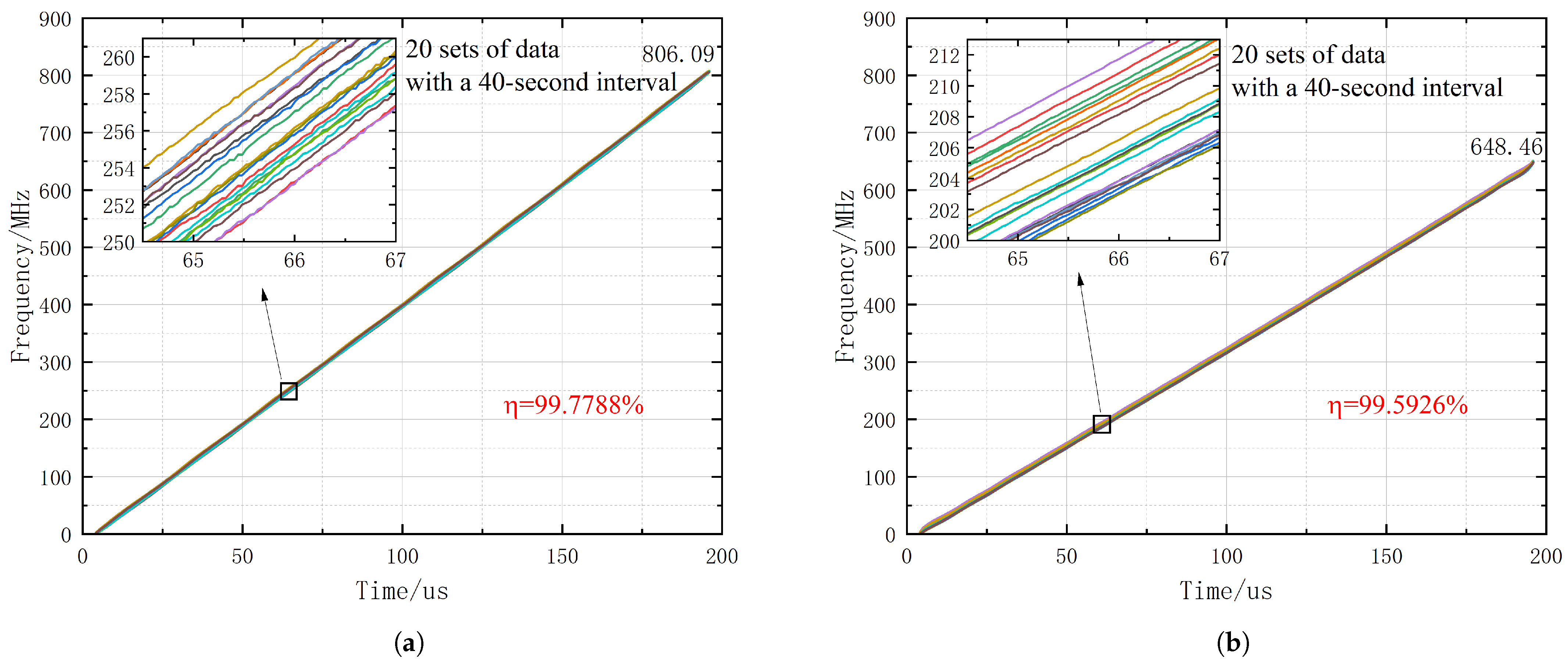
As previously mentioned, the derivations presented in this paper are based on the prerequisite that the optical frequency sweep curve output by the laser exhibits excellent repeatability. To illustrate this issue, we conduct the following repeatability experiment. The AFG generates a triangular wave with a frequency of 2.5 KHz and an amplitude of 10 Vpp, causing the laser to generate an optical frequency sweep signal with a bandwidth of approximately 540 MHz. The MZI has its channel-b replaced with an alternative fiber b1. The BPD receives the beat signal ${\varphi }_{b1}\left(t\right)$, which is then displayed on the OSC. The PC is responsible for calculating the optical frequency sweep curve. We collect a set of beat signal data from the oscilloscope every 40 s without replacing the alternative fiber. A total of 20 sets of data are collected, resulting in a total time expenditure of 800 s. 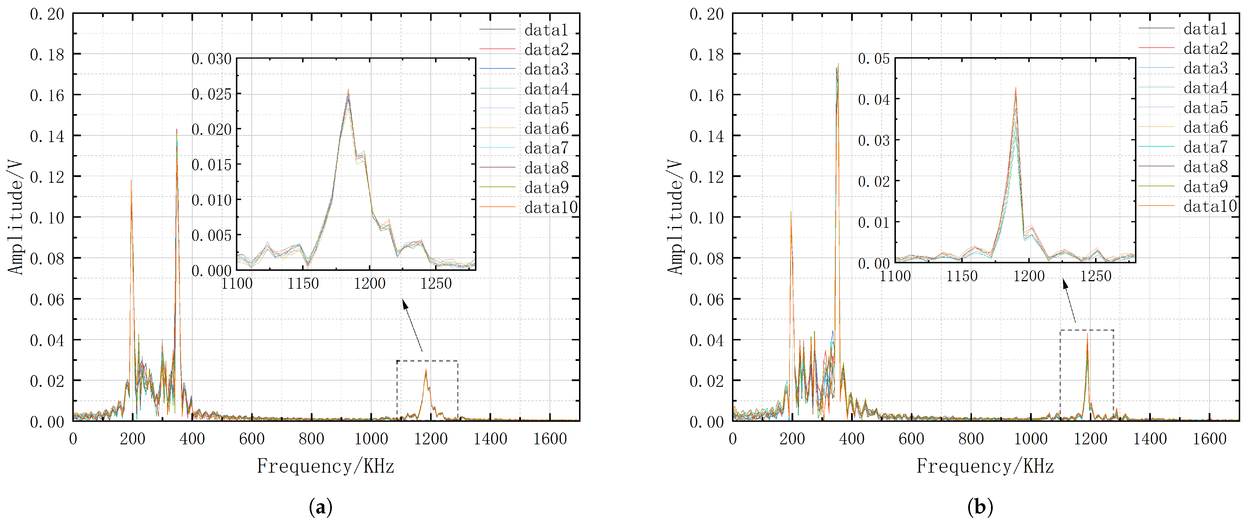Based on the derivations presented earlier, and by employing the Hilbert transform (HT) and utilizing the accurately measured delay ${\tau }_{b1}$ of the alternative fiber instead of the total delay difference ${\tau }_{b1\_total}$ of the MZI, we can directly calculate 20 sets of optical frequency sweep curves using Equation (2). Placing these curves on the same coordinate system allows for the observation of the repeatability of the optical frequency sweep signal output by the laser. The results are depicted in Figure 3a. In this paper, only the beat signals generated during the up ramp of the triangular wave are extracted for the calculation of the optical frequency sweep curves (the calculation for the down ramp is analogous). From the results, it is observed that since the value ${\tau }_{b1}$ used for calculation is less than ${\tau }_{b1\_total}$, the resulting optical frequency sweep curves exhibit a frequency sweep bandwidth larger than the preset value. However, this does not affect the assessment of the repeatability measurement results for the optical frequency sweep. If the repeatability is sufficiently good, despite the slightly broader frequency sweep bandwidth, ideally, the 20 sets of optical frequency sweep curves should perfectly coincide. In fact, owing to the inherent stability issues of the laser and the impact of environmental factors such as temperature and vibration, they do not perfectly align but instead form a set of lines with a certain breadth, indicating a range of variations [29].

To ascertain their repeatability more clearly, we perform the following calculations: By averaging the 20 sets of optical frequency sweep curves and fitting them to one curve, which is considered the true value $y_i$ of the optical frequency sweep signal output by the laser, and each individual set is regarded as a predicted value $\widehat{y_i}$. Consequently, the root mean square error (RMSE) can be calculated for each set by $v_{s,rmse}=\sqrt{{\sum }_{i=1}^n{(y_i-{\widehat{y}}_i)}^2/n}$, where n is the number of sampling points. The RMSE for each set is then averaged to obtain the mean RMSE, which is given by ${\overline{v}}_{s,rmse}=v_{s,rmse}/20$, Thus, the repeatability of the optical frequency sweep signal output by the laser can be defined by this mean RMSE, serving as a quantitative indicator of the signal’s consistency across the individual sets. The repeatability $\eta$ is defined as

$$\eta =(1-{\displaystyle \frac{{\overline{v}}_{s,rmse}}{BW}})\times 100\%$$

(6)

where $BW$ is the frequency sweep bandwidth. This definition measures the relative deviation of the optical frequency sweep signal at different times as a proportion of the entire frequency sweep bandwidth $BW$. Given that $BW$ is already determined, the smaller the mean ${\overline{v}}_{s,rmse}$ of 20 sets of RMSE, the higher the repeatability of the optical frequency sweep signal.

The experimental data analysis indicates that when b1 is used in the MZI, the repeatability of the measured 20 sets of optical frequency sweep curves is 99.7788%. Similarly, when b2 is used in the MZI, a set of beat data is collected every 40 s, and 20 sets of data are collected and used to calculate the optical frequency sweep curves. The results, plotted on the same coordinate system as shown in Figure 3b, demonstrate a repeatability of 99.5926%.

The calculated results indicate that the repeatability of the frequency-modulated signal output by the laser is very good, meaning that the optical frequency sweep signal does not significantly change with time or remains stable over a short period. Under these conditions, the proposed method for measuring the optical frequency sweep using alternative fibers in a calibration-free MZI is effective, thereby ensuring the accuracy of the nonlinearity measurement of the optical frequency sweep.

3.2. The Nonlinearity Measurement

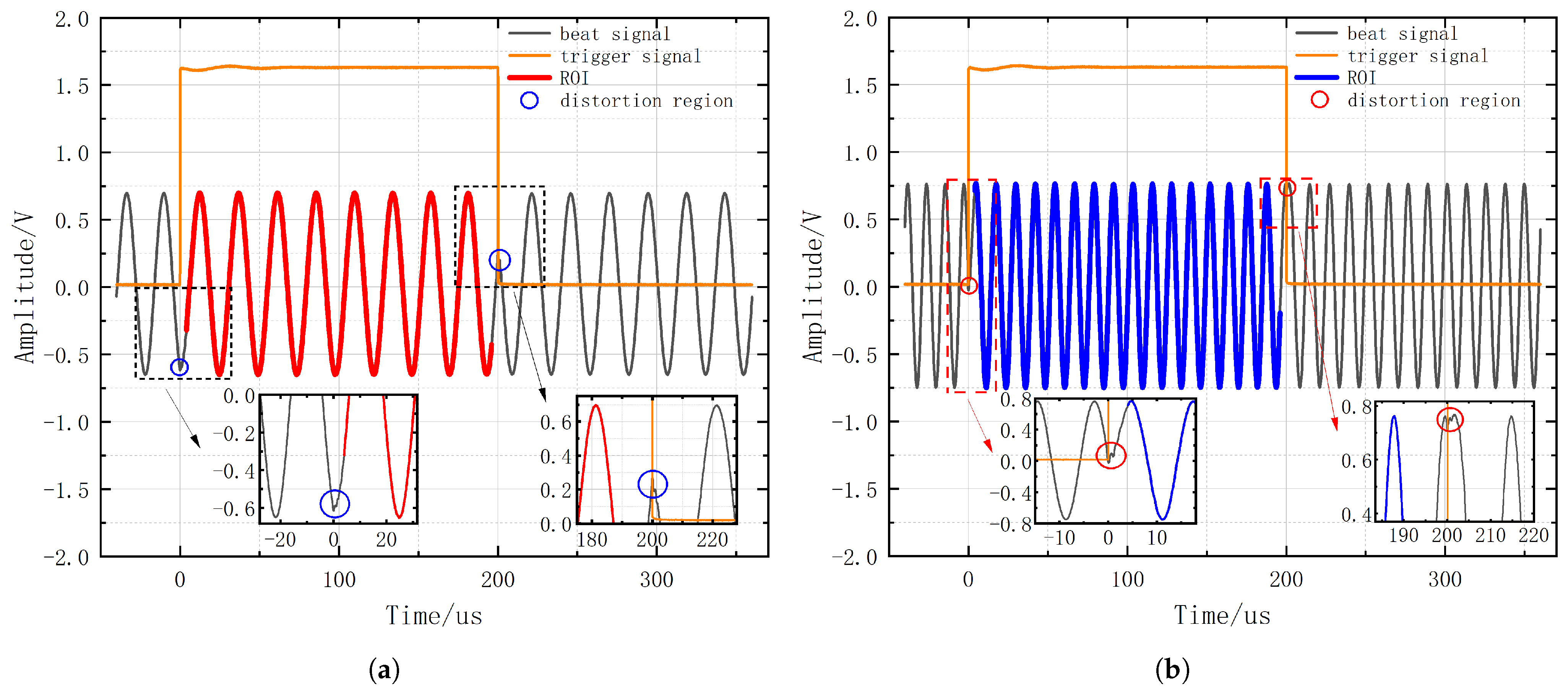
Within the MZI, channel-b is equipped with the alternative fiber b1. The BPD receives the beat signal ${\varphi }_{b1}\left(t\right)$, which is then displayed on the OSC. To more precisely calculate the optical frequency sweep curve and its nonlinearity, the OSC’s sampling rate is set to 25 MS/s, with a single sampling record length of 10,000 points. The single-shot sampling result of the beat signal is depicted in Figure 4a. The beat signal corresponding to the high-level state (approximately 1.6 V) of the trigger signal is generated during the up ramp of the frequency sweep, while the beat signal corresponding to the low-level state (0 V) of the trigger signal is generated during the down ramp. It can be observed that the beat signal exhibits noticeable distortion near the transition of the up and down ramps. The distortion is due to the significant frequency sweeping nonlinearity at the transition of the up and down ramps. In order to mitigate the impact of this distortion on the computational accuracy of the optical frequency sweep signal, 100 sampling points are cut off respectively at the beginning and end of the beat signal corresponding to the up ramps in the experiment, totaling a sampling time of 8 μs. For a frequency sweep up ramp of 200 μs, a region of interest (ROI) of 192 μs is used for evaluating nonlinearity, which accounts for 96% of the frequency sweep up ramp. Utilizing the HT, the PC computes an optical frequency sweep curve $v_{b1}\left(t\right)$ from the ROI of the beat signal by Equation (2), employing the accurately measured delay ${\tau }_{b1}$ to act as the total delay difference ${\tau }_{b1\_total}$ between the two arms of the MZI. Subsequently, with the experimental parameters remaining unchanged, the alternative fiber b2 is used in the MZI, and the beat signal obtained from a single-shot sampling is shown in Figure 4b. Similarly, by using the delay ${\tau }_{b2}$ as the total delay difference ${\tau }_{b2\_total}$ between the two arms of the MZI, another optical frequency sweep curve $v_{b2}\left(t\right)$ is calculated by Equation (3). Finally, the ROI data of the beat signals obtained in the first two steps are subtracted from each other, and then the optical frequency sweep curve $v\left(t\right)$ output by the laser can be calculated from Table 1 and Equation (5).

The three optical frequency sweep curves $v_{b1}\left(t\right)$, $v_{b2}\left(t\right)$, and $v\left(t\right)$ are placed in the same coordinate system, as shown in Figure 5. It is evident that when the alternative fibers are used individually for the calculation of the optical frequency sweep curve, the frequency sweep bandwidths are 806.09 MHz (corresponding to b1) and 648.46 MHz (corresponding to b2), respectively. Compared with the preset value of approximately 540 MHz, these values are somewhat higher. This is because the delays ${\tau }_{b1}$ and ${\tau }_{b2}$ are smaller than the total delay difference; i.e., the delay ${\tau }_{other}$ is ignored. The final calculated optical frequency sweep curve $v\left(t\right)$ has a frequency sweep bandwidth of 541.88 MHz, which is in accordance with the experimental expectations. This indicates that we do not necessarily need to know the exact value of the total delay difference between the two arms of the MZI to obtain the optical frequency sweep curve output by the laser, thereby validating the calibration-free MZI measurement method presented in this paper.

Once the optical frequency sweep curve is obtained, it can be used to calculate the nonlinearity. Regarding the nonlinearity of the optical frequency sweep curve output by the laser, different criteria have been proposed by various sources. However, two definitions are currently widely utilized. One of them is the nonlinearity R, the expression of which is given by [30]

$$R={\displaystyle \frac{v_{nl,rms}}{BW}}\times 100\%$$

(7)

where $v_{nl,rms}=\sqrt{{\sum }_{i=1}^n{(v_i-{\tilde{v}}_i)}^2/n}$ is the root mean square of residual frequency errors, $v_i$ is the optical frequency points obtained from a single measurement of the optical frequency sweep curve, ${\tilde{v}}_i$ is the optical frequency points of the fitting curve obtained by the linear function fitting of $v_i$, n is the number of sampling points, and $BW$ is the frequency modulation bandwidth. $v_{nl,rms}$ reflects the frequency deviation error between the measured optical frequency sweep curve and the fitting curve. The nonlinearity R presents the proportion of the optical frequency sweeping nonlinearity error to the sweep bandwidth in a percentage form, providing a clear and intuitive measure of the impact of nonlinearity errors on the bandwidth. Consequently, the nonlinearity R of the measured optical frequency sweep curve $v\left(t\right)$ in the experiment can be calculated to be 0.2113%.

The other is the relative nonlinearity $1-r^2$, the expression of which is given by [13]

$$r^2=1-{\displaystyle \frac{s{s}_{res}}{s{s}_{tot}}}$$

(8)

where $s{s}_{res}={\sum }_{i=1}^n{(v_i-{\tilde{v}}_i)}^2$ is the sum of residual squares, $s{s}_{tot}={\sum }_{i=1}^n{(v_i-\overline{v})}^2$ is the total sum of squares, $v_i$ and ${\tilde{v}}_i$ are the same as above, $\overline{v}=v_i/n$ is the mean value of $v_i$, and n is the number of sampling points. $s{s}_{res}$ reflects the deviation between $v_i$ and ${\tilde{v}}_i$, and $s{s}_{tot}$ reflects the deviation between $v_i$ and $\overline{v}$. The relative nonlinearity $1-r^2$, from a statistical perspective, uses the mean as a benchmark error, observing whether the frequency deviation error is greater or less than the mean benchmark error to assess the nonlinearity. The smaller the value, the better the linearity of the optical frequency sweep curve. Consequently, the relative nonlinearity $1-r^2$ of the measured optical frequency sweep curve $v\left(t\right)$ in the experiment can be calculated to be 5.3560 × 10⁻⁵.

According to the analysis and derivation from the nonlinearity measurement experiment, once we obtain an optical frequency sweep curve $v\left(t\right)$, with the beat signal ${\varphi }_{b1}\left(t\right)$ measured in this experiment, we can retro-calculate the accurate total delay difference ${\tau }_{b1\_total}$ in the MZI by Equation (2), i.e., ${\tau }_{b1\_total}=2\pi v_s\left(t\right)/{\varphi }_{b1}\left(t\right)$. That is to say that when utilizing the alternative fiber b1, ${\tau }_{b1\_total}$ is 14.592 ns. Similarly, when utilizing the alternative fiber b2, ${\tau }_{b2\_total}$ is 29.248 ns. In this way, the total delay differences corresponding to the two alternative fibers in the MZI are known quantities, facilitating the use of this interferometer for subsequent extended experimental research, such as the frequency sweep linearization of the FMCW LIDAR light source, speed and distance measurement, and three-dimensional imaging.

3.3. The Accuracy Verification

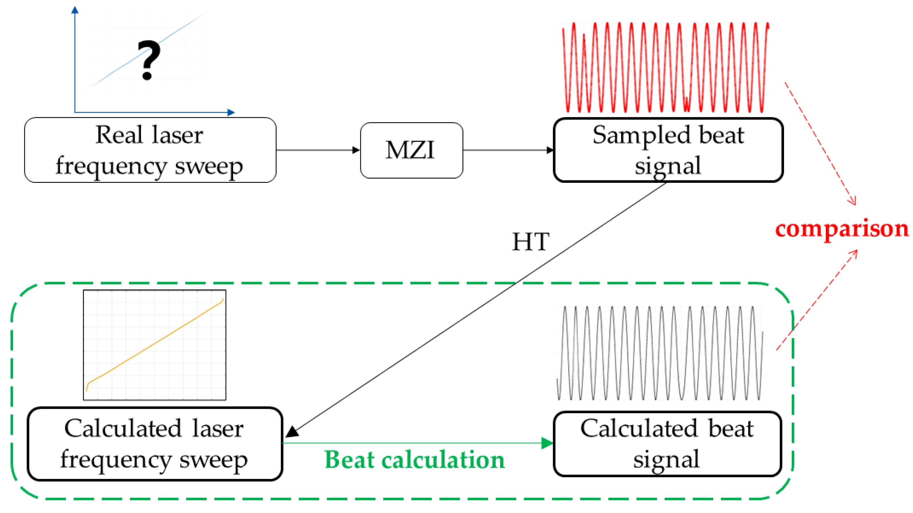
As shown in Figure 6, the measured optical frequency sweep curve in the experiment is derived by down-converting the optical frequency to an intermediate frequency, known as the beat signal, in the MZI and then performing an HT on the beat signal. Since the optical frequency sweep signal output by the laser is difficult to sample directly, the accuracy of the measured optical frequency sweep curve cannot be directly assessed. However, it can be affirmed that the beat signal sampled through the MZI is accurate and reliable. Therefore, the optical frequency sweep curve obtained from the experiment can be subjected to numerical calculations and simulations within software to emulate the beat signal detected by the detector. By comparing the calculated beat curve with the experimentally sampled beat signal, if there is a good agreement between them, it indicates that the measured optical frequency sweep curve in the experiment is accurate. This validation process is crucial for confirming the fidelity of the experimental results and ensuring the reliability of subsequent analyses and applications.

It has been reported that the accuracy of the measured optical frequency sweep curve is verified by performing polynomial fitting on the measured optical frequency sweep curve and then integrating the result to obtain the optical frequency sweep phase, thereby performing the beat reproduction to compare whether the calculated beat spectrum is consistent with the sampled beat spectrum [31]. Based on this method, we do not perform polynomial fitting but instead interpolate the measured optical frequency sweep curve, and then integrate the result to obtain the optical frequency sweep phase. At last, we simulate the process of an optical frequency sweep signal being split, delayed, and mixed in the MZI, using the optical frequency sweep phase, to replicate the sampled beat signal. The specific procedure is as follows:

Through the experiments and calculations of the previous subsection, we are able to obtain the optical frequency sweep curves $v_{b1}\left(t\right)$ and $v_{b2}\left(t\right)$, as well as the total delay difference ${\tau }_{b1\_total}$ and ${\tau }_{b2\_total}$ between the two arms of the MZI. 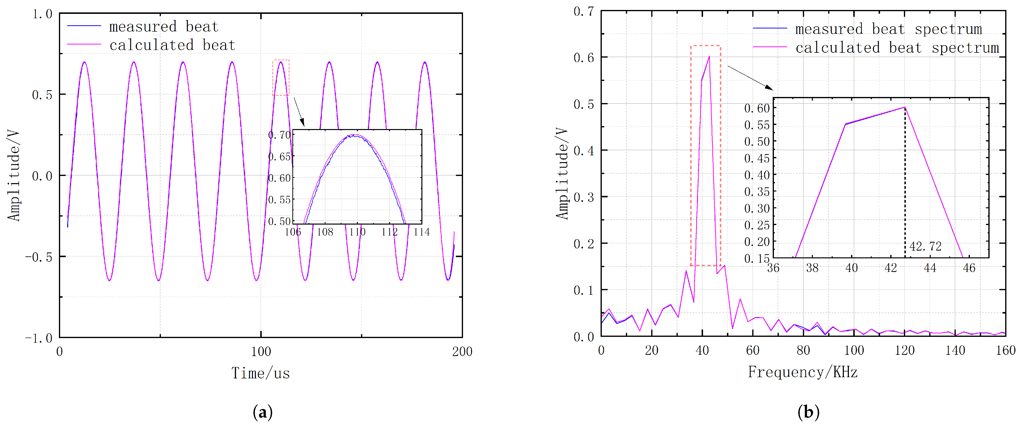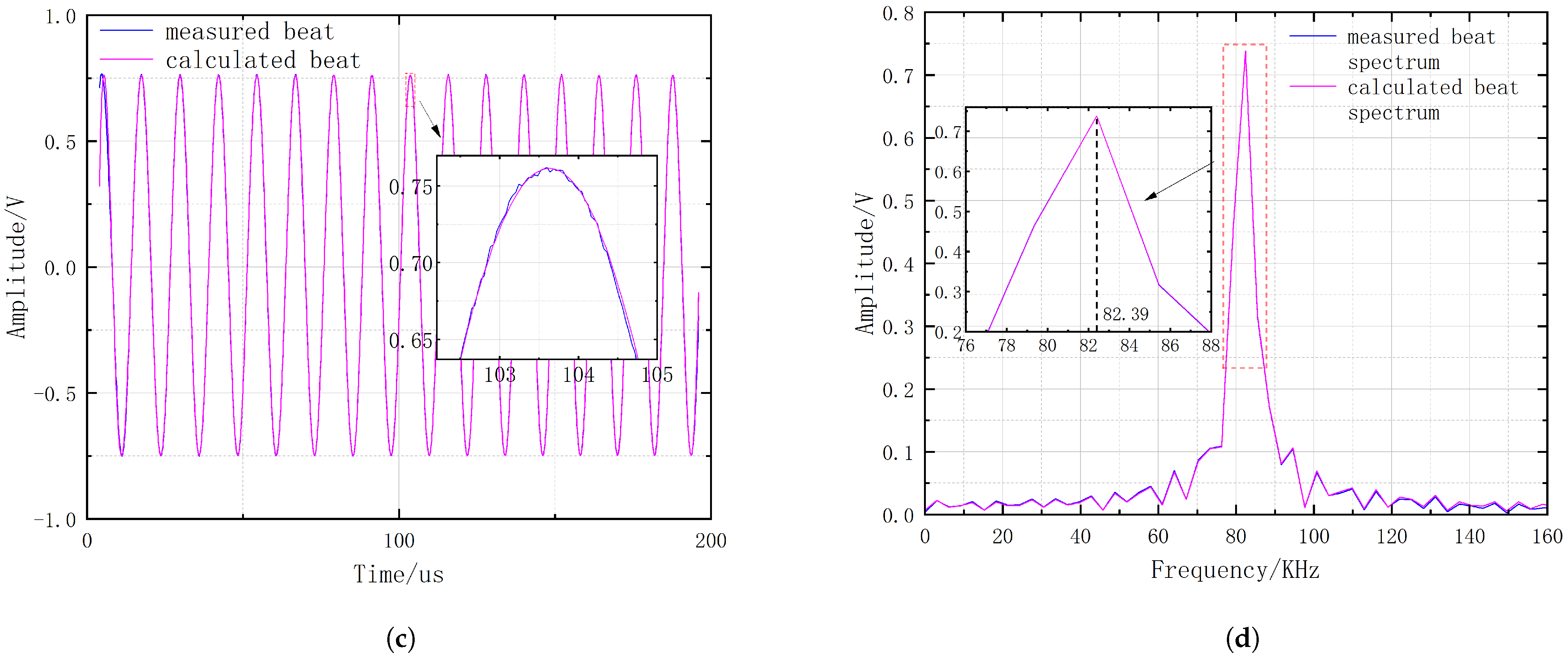Given the OSC’s sampling interval of 40 ns, to enhance the point density of the optical frequency sweep curve, we perform interpolation on $v_{b1}\left(t\right)$ and $v_{b2}\left(t\right)$ with an interpolation interval of 8 ps, which increases the data points to 5000 times the original amount, and then integrate the results to derive the optical frequency sweep phase. Using the high-density beat phase difference allows for the reproduction of the beat signal. In this process, the delay precision is also improved to the thousandths with the increase in data points, thereby enhancing the accuracy of reproduction. In order to compare with the sampled beat signal, it is also necessary to perform downsampling on the calculated beat curve to ensure that their data point densities are consistent. Since the optical frequency sweep curve obtained from the previous experiment was calculated from the ROI of the beat signal corresponding to the frequency sweep up ramp, the beat curve reproduced here will also only correspond to the up ramp of the frequency sweep. The experimentally sampled beat signal and the calculated beat curve are plotted on the same coordinate system for comparison. To more clearly observe the degree of agreement between them, their beat spectra are also compared on the same coordinate system. The results are shown in Figure 7, demonstrating an effect that is comparable to the polynomial fitting methods used in reported studies. In the time domain, they are found to almost coincide; in the frequency domain, their peak frequencies, that is, the beat frequencies, are in complete agreement. There is only a minor difference in amplitude between them in both the time and frequency domain. The beat frequencies corresponding to the alternative fibers b1 and b2 are 42.72 kHz and 82.39 kHz, respectively. Indeed, whether in the time domain or the frequency domain, there is a close match between the beat signal sampled from the experiment and the beat curve derived from the calculations. This confirms the validity of the optical frequency sweep curve and its nonlinearity data measured in the previous experimental section.

3.4. The Temperature Insensitivity Verification

As mentioned above, this method is virtually unaffected by fluctuations of the experimental ambient temperature. To illustrate this issue, we conduct the following temperature insensitivity verification experiment.

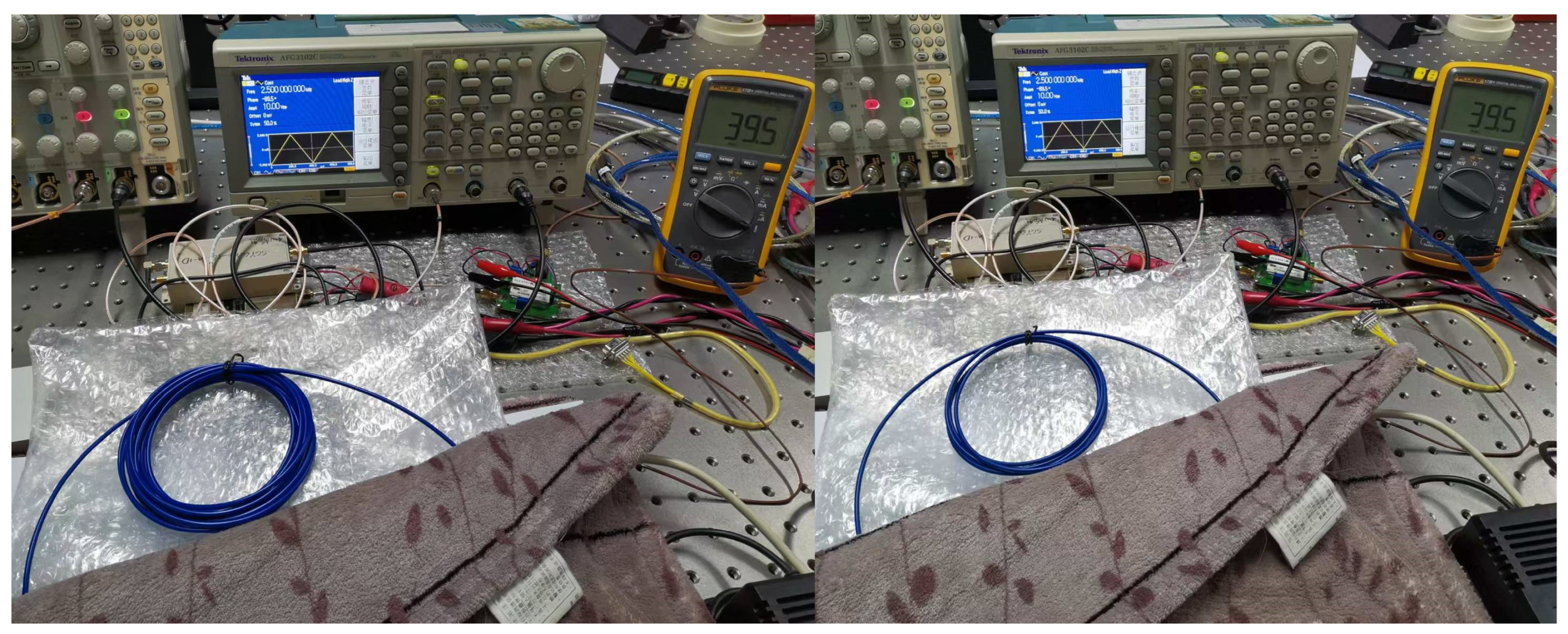
The procedures of the temperature insensitivity verification experiment are essentially consistent with those described in Section 3.2. The difference lies in the fact that we place the fibers, which are not involved in the final calculation of the frequency sweep curve—specifically, the fiber connecting the optical components—into a heating pad. Through the action of the heating pad, the fibers are subjected to different temperatures to assess the adaptability of the method presented in this paper for measuring the frequency sweep curve under various temperature environments. Prior to the activation of the heating pad, we measure the ambient temperature of the experimental setup, as shown in Figure 8, where the ambient temperature, that is, the room temperature, is 24.1 °C. Subsequently, the heating pad envelops the fibers and heats them to a specific temperature (note that the two alternative fibers are kept in a room-temperature environment). Once the temperature stabilizes, the two alternative fibers are alternately inserted to one arm of the MZI for two separate measurements of the frequency sweep curve, as depicted in Figure 9. Finally, based on the calculations described earlier, the final optical frequency sweep curve could be derived.

Through this experimental process, we control the temperature inside the heating pad at 24.1, 30.4, 39.5, and 44.0 °C to conduct the frequency sweep measurements (due to equipment limitations, the highest experimental temperature could only reach 44.0 °C). The final frequency sweep curves calculated are shown in the same coordinate system in Figure 10. The repeatability of the four frequency sweep curves can be calculated using Equation (6) to be 99.8235%.

Critically, the method for measuring the optical frequency sweep curve presented in this paper first places the two alternative fibers in a room-temperature environment and then alternately inserts them to one arm of the MZI during measurement. Despite the fact that the lengths or delays of the fibers connecting other optical components may be subject to changes due to temperature fluctuations during the experiment, they are not involved in the calculation of the optical frequency sweep curve. This method does not require prior calibration of the MZI’s arm length difference; it only necessitates knowledge of the delays of the two alternative fibers, with no special requirements for other configurations of the interferometer. This not only enhances the flexibility of the experimental setup in facing various measurement environments but also, importantly, makes it minimally susceptible to the effects of environmental temperature fluctuations, which further demonstrates the accuracy of the optical frequency sweep curves measured in this paper.

4. The Ranging Results with Pre-Distortion

To further verify the accuracy of the measured frequency sweeping nonlinearity presented in this paper, we utilized an iterative learning pre-distortion method, as previously reported, to correct the frequency-modulated signal of the laser [13]. This method is effective for enhancing the linearity of the laser’s frequency sweep, which is critical for applications such as FMCW LIDAR systems that demand high measurement precision. The iterative learning control (ILC) process involves multiple iterations to achieve the desired level of linearity in the laser’s frequency sweep. By comparing the frequency sweep before and after the pre-distortion, the efficacy of the pre-distortion correction can be assessed, ensuring that the laser’s frequency modulation closely approximates the ideal linear frequency sweep. This validation process is vital for the dependable performance of sophisticated laser-based measurement systems.

A comparison of the optical frequency sweeping nonlinearity before and after the pre-distortion is shown in Figure 11. The 20 us sampling points are cut off respectively at the beginning and end of the frequency sweep half-period, leaving a 160 us ROI that is used to calculate the root mean square of the residual frequency errors $v_{nl,rms}$. It can be observed that before the pre-distortion, the nonlinearity of the optical frequency sweep is apparent, with $v_{nl,rms}$ being 0.6872 MHz, which can be reduced to 0.0475 MHz after applying the pre-distortion. Additionally, we measure the nonlinearity every 3 min to monitor the stability of the laser’s frequency sweeping nonlinearity after the pre-distortion, over a total period of 30 min. As shown in Figure 11, the $v_{nl,rms}$ of the frequency sweep curve could be maintained within 0.1 MHz after the pre-distortion. Compared with the reported results, using the same iterative algorithm for the pre-distortion, our ability to control the nonlinearity within 0.1 MHz is precisely due to the higher accuracy of the measured optical frequency sweeping nonlinearity in this paper, which allows for better suppression effects in the pre-distortion and in turn highlights the importance of measuring the frequency sweeping nonlinearity of FMCW LIDAR light sources.

Subsequently, we constructed a basic FMCW LIDAR ranging system, as shown in Figure 12. The frequency-modulated light output by the laser is divided into 90% detection light and 10% local oscillator light. The detection light is transmitted and received by a collimator, and the echo signal carrying the target distance information is mixed with the local oscillator light to form a beat signal. This beat signal is received by a balanced photodetector (BPD) and displayed on an oscilloscope (OSC).

Adjusting the parameters of the triangular wave modulation signal allows the laser to output a frequency-modulated signal with a frequency sweep bandwidth of 550 MHz and a frequency sweep period of 400 us. The specific adjustments would involve setting the modulation signal’s amplitude and frequency to match the desired sweep characteristics. The sampling parameters of the OSC remain unchanged. We conduct a ranging experiment on a target at 45 m, performing 10 collections and processing the target echo beat signals before and after the pre-distortion, respectively. The results of the beat spectra plotted on a linear coordinate system are shown in Figure 13. The average of the 10 beat spectra before and after the pre-distortion is calculated and compared on the same linear coordinate system, as shown in Figure 14. The two higher peaks on the left side of the figure are attributed to the optical crosstalk produced by the detection light at the circulator and the specular reflection at the collimator, respectively. The lower peak on the right side is produced by the target echo. Therefore, the frequency difference between the specular reflection peak and the target echo peak corresponds to the target range, which is 836.182 kHz. According to the FMCW LIDAR ranging formula [32]

$$D={\displaystyle \frac{1}{2}}c\tau ={\displaystyle \frac{cT}{4B}}·f_b$$

(9)

where D is the distance to be measured, $\tau$ is the round-trip time of the detection light from the collimator to the target, c is the speed of light in a vacuum, T is the frequency sweep period of the frequency-modulated triangular wave, B is the frequency sweep bandwidth, and $f_b$ is the beat of the target echo. The calculated distance is 45.610 m, which is essentially consistent with the distance measured using a laser rangefinder. From Figure 14, it can be observed that the spectral broadening of the target echo beat due to the nonlinearity of the laser’s frequency sweep is reduced after the pre-distortion. The full width at half maximum (FWHM) decreases from 25.635 KHz to 9.736 KHz, which is a reduction by a factor of 2.633. Additionally, after the pre-distortion, the amplitude of the target peak increases by 3.751 dB.

Based on the theory of FMCW LIDAR ranging, the longer the detection distance, the more severe the broadening of the target echo beat spectrum caused by the nonlinearity of the laser frequency sweep, and the greater the impact on the system’s ranging resolution. The aforementioned ranging experiments are only conducted at a distance of 45 m, and the improvement in the target echo beat spectrum broadening before and after the pre-distortion is not significant. To further demonstrate the correction effect of the pre-distortion on the nonlinearity of the laser frequency sweep, we conduct kilometer-level ranging experiments using our ranging system, as shown in Figure 15a. With the same experimental procedures and data processing methods, the results are depicted in Figure 15b. As can be seen, the target echo beat is 22.412 MHz. Using Equation (9), the target distance can be calculated to be 1.222 km, which is consistent with the distance shown on the map webpage (https://ditu.amap.com/). After the pre-distortion, the FWHM of the target echo beat spectrum decreases from 747.880 kHz to 22.012 kHz, a reduction of 33.976 times. The amplitude of the main lobe of the target peak increases by 6.933 dB, while the amplitude of the side lobe is maximally suppressed by 27.287 dB. This will inevitably enhance the resolution and accuracy of the FMCW LIDAR ranging system at kilometer-level distances.

Actually, all the experimental analyses in this section are made possible by the high accuracy of the measured optical frequency sweeping nonlinearity from the previous sections. In other words, the calibration-free MZI measurement method for optical frequency sweeping nonlinearity presented in this paper is accurate and reliable enough to ensure that the pre-distortion of the laser’s frequency sweep has a significant suppressive effect on the spectrum broadening of the beat.

5. Discussion

In this paper, we introduced an innovative approach to measuring the nonlinearity of the optical frequency sweep in FMCW LIDAR systems, utilizing a calibration-free Mach–Zehnder interferometer. This method, which employs two alternative fibers with precisely known delays, has proven to be highly accurate in characterizing the laser source’s frequency sweep curve. Our findings underscore the significance of measuring frequency sweeping nonlinearity for enhancing the resolution and accuracy of FMCW LIDAR systems. The nonlinearity R measured in our experiments was 0.2113%, a value that, while small, can have substantial implications for long-range LIDAR applications where even minor deviations can lead to significant errors in distance measurement. The relative nonlinearity $1-r^2$ of 5.3560 × 10⁻⁵ further highlights the subtle deviations from an ideal linear sweep, which are critical to address for high-precision sensing.

The discussion of our results must be contextualized within the broader scope of LIDAR technology and its diverse applications. FMCW LIDAR systems are increasingly integral to fields such as autonomous navigation, topographical mapping, and environmental monitoring [3,4,33]. The precision of these systems is fundamentally dependent on the quality of the light source’s frequency sweep. Nonlinearities can introduce target echo beat spectrum broadening and diminish the system’s ability to discern closely spaced objects, thereby undermining the overall performance of the LIDAR system [13].

A key advantage of our method is its simplicity and adaptability. By leveraging two short polarization-maintaining fibers with known delays, we have circumvented the need for complex and sensitive calibration procedures. This method does not require additional auxiliary interferometers or similar devices, making it suitable for various fiber MZIs. This simplification not only expedites the setup but also minimizes the susceptibility to environmental perturbations, such as temperature-induced fluctuations. The portability of our method is further enhanced by the ease with which the fibers can be transported and integrated with any fiber-based MZI, facilitating its use in field applications where equipment must be mobile and versatile.

However, our study is not without its limitations. The experimental validation was conducted under controlled laboratory conditions, and the method’s robustness in uncontrolled, real-world environments remains to be evaluated. Additionally, while our method exhibits temperature insensitivity, long-term field tests are necessary to confirm its constancy over extended periods.

Future research should focus on the real-time integration of this method with operational LIDAR systems to assess its practicality in dynamic and variable conditions. Furthermore, exploring the method’s compatibility with other interferometer types could broaden its utility in the field of optical sensing. The potential of this technique to influence the development of next-generation LIDAR systems, particularly those incorporating solid-state lasers and photonic integrated circuits, should also be a subject of future inquiry.

In conclusion, our calibration-free MZI method for measuring the nonlinearity of the optical frequency sweep in FMCW LIDAR systems, due to Its simplicity, accuracy, and adaptability, positions it as a valuable tool for optimizing the performance of LIDAR systems across a spectrum of applications. As the demand for high-precision LIDAR systems escalates, the ability to precisely measure and correct for frequency sweep nonlinearities will become increasingly vital.

6. Conclusions

In this paper, we propose and demonstrate an improved method, based on a calibration-free MZI with two alternative fibers whose delays are accurately measured, for accurately measuring the laser optical frequency sweep curve. According to the widely used measurement standard of frequency sweeping nonlinearity, the nonlinearity of the frequency swept light source used in the experiment is calculated to be 0.2113 %, and the relative nonlinearity is 5.3560 × 10⁻⁵. By comparing the calculated beat curve with the sampled beat signal in the time and frequency domain, the accuracy of the measured optical frequency sweep curve is verified. The temperature insensitivity verification experiment conducted at four different temperatures demonstrates that the method described in this paper is virtually unaffected by environmental temperature fluctuations. The FMCW LIDAR ranging results with a light source pre-distortion at both 45 m and 1.2 km confirm the accuracy and reliability of the measured optical frequency sweep curve.

Compared with the reported methods, the method presented in this paper avoids the complexities of calibration procedures, is simple to operate, and does not require additional interferometers or other devices, making it suitable for various fiber MZIs. When the experimental setup needs to be relocated, only the two alternative fibers need to be carried, which enhances the portability of our method. Moreover, the measurement accuracy is less susceptible to ambient temperature, making it applicable to the frequency sweep linearization of the FMCW LIDAR light source, range and velocity measurement, three-dimensional imaging, and other related research areas.