Article

Research on Key Influencing Factors of Ecological Environment Quality in Barcelona Metropolitan Region Based on Remote Sensing

Centre for Land Policy and Valuations (CPSV), Barcelona School of Architecture (ETSAB), Universitat Politècnica de Catalunya, 08028 Barcelona, Spain
*
Author to whom correspondence should be addressed.
Remote Sens. 2024, 16(24), 4735; https://doi.org/10.3390/rs16244735
Submission received: 31 October 2024 / Revised: 6 December 2024 / Accepted: 16 December 2024 / Published: 18 December 2024

Abstract

:
With the rapid development of urbanization, the ecological environment is being degraded. Taking the Barcelona Metropolitan Region as an example, this paper developed an ecological environment quality-assessment system suitable for different times and regions, based on remote sensing, to evaluate the quality of the ecological environment from 2006 to 2018. We also built various ordinary least squares models to analyze multiple variables affecting the ecological environment. Finally, the characteristic triangular spatial structure was used to explain the interaction between the two key variables. The results showed that the ecological quality was unevenly distributed. The largest green space contributed the most benefits but was decreasing and becoming fragmented. NDVI (normalized difference vegetation index) was the most significant natural variable related to the distribution of green space. Precipitation was the most closely related climate factor to NDVI. There was a complex two-way interaction mechanism between the two, and its boundary value was getting higher and higher. In conclusion, the environmental quality of the BMR needs improvement. The characteristic triangle can effectively explain the interaction mechanism between precipitation and NDVI. This study deeply analyzes how various factors affect environmental quality from both the global and internal perspectives and provides a scientific basis for urban ecological management and sustainable development.

1. Introduction

Over the past few decades, environmental assessment has emerged as a critical component of environmental management, garnering increasing attention [1]. The impact of human activities on environmental changes and the pivotal role of environmental assessment in understanding these processes are now widely acknowledged [2]. In today’s rapidly urbanizing and industrializing world, human activities have severely damaged the ecological environment, exacerbating issues such as soil erosion, land salinization, desertification, and a sharp decline in biodiversity [3,4]. Concurrently, the degradation of the ecological environment has led to more frequent natural disasters and extreme climatic events, including floods, droughts, global warming, and heatwaves [5,6,7]. A healthy ecological environment forms the foundation of sustainable social development and human survival. The continued deterioration of ecological conditions has significantly impacted societal development and public health. Addressing ecological and environmental issues must go hand-in-hand with urban development, economic growth, and scientific advancement. Only through this balanced approach can we achieve harmonious coexistence between humanity and nature, reduce the frequency of natural disasters and extreme weather events, safeguard public health, and ensure the sustainable use of natural resources [8].
The scientific evaluation of the ecological environment and the rational optimization of its patterns are not only prominent topics in climate and environmental research but also pressing demands for ecological economic development and the construction of ecological civilization [9]. Currently, satellite-based remote sensing earth-observation systems are widely applied in ecological environment studies due to their macro-scale, rapid, and real-time advantages. The use of various remote sensing indicators to monitor and assess natural forests, grasslands, urban impervious surfaces, water bodies, and ecosystems at regional scales has become integral to ecological protection efforts [10]. With advancements in “3S” technologies (remote sensing, geographic information systems, and global positioning systems), many researchers have employed RS and GIS technologies to acquire ground information, combining mathematical models and statistical analysis to conduct comprehensive evaluations of the ecological environment across diverse regions and scales [11,12]. For example, in 2009, Ivits et al. used SPOT imagery and the Normalized Difference Vegetation Index (NDVI) as an ecological indicator to evaluate forest and farmland bird habitats in China [13]. Similarly, Marllu J. et al. developed an urban ecological environment-evaluation system, incorporating vegetation sensitivity and ecological isolation indices, providing critical insights for urban land-use planning [14]. In 2013, Xu Hanqiu introduced the Remote Sensing Ecological Index (RSEI), which integrates four key indicators: vegetation index, humidity component, surface temperature, and soil index. The index employs principal component analysis to provide a comprehensive representation of regional ecological conditions. Xu used the RSEI alongside China’s traditional EI to study areas with severe soil erosion in Fujian Province, enabling dynamic analysis and predictive assessments that addressed the limitations of the EI [15]. Recent research has further expanded the application of remote sensing in ecological studies. Wang Zi (2021) analyzed the ecological quality of the Chahan Nur Basin from 1992 to 2020 using Landsat imagery and saline-alkali land-specific indicators [8]. Hou Yifeng et al. (2022) explored the evolution of land cover changes in the Tarim River Basin and assessed the ecological contributions of different land-use transformations over three decades [16]. Numerous studies have underscored the critical role of NDVI in ecological monitoring. Wessels et al. (2004) demonstrated a positive correlation between NDVI and soil health, using it to evaluate ecosystem quality in northern South Africa [17]. NDVI has been widely applied to detect seasonal and long-term vegetation trends, assess ecosystem health, and monitor ecosystem restoration efforts [18,19,20]. For instance, Goward and Prince established its utility as a proxy for vegetation’s net primary productivity (NPP) [19], while Ren Jie (2020) revealed that lower NDVI values correspond to higher ecological sensitivity in the western Yili Basin [21]. Urban agglomerations have also become a focal point of ecological-quality research. Zhang Yi et al. (2022) analyzed the Changsha–Zhuzhou–Xiangtan metropolitan area using the RSEI and structural equation modeling to explore the interactions between natural and anthropogenic factors [22]. In 2023, Zhang Lifang employed multivariate regression models to investigate the spatial heterogeneity of driving forces affecting urban ecological quality in China [23]. Huang Min et al. (2024) used a “point-line-surface” approach to study the spatiotemporal dynamics of land-use and ecological patterns in the Poyang Lake Ecological Zone [24]. However, despite these advancements, there remains no unified standard for evaluating ecological quality. Commonly used indices, such as land weight indices, are often numerical and limited to static regional descriptions, making them inadequate for analyzing spatial and temporal changes [8,11,12,13,14,15,16,17,18,19,20,21]. Moreover, existing studies lack process-based, dynamic ecosystem analyses and often rely on highly subjective indicator constructions, introducing constraints for large-scale evaluations [22,23,24].
Numerous studies have highlighted that NDVI is a critical indicator for assessing and reflecting a region’s ecological environment quality. Consequently, it is essential to analyze the factors that directly influence NDVI and indirectly regulate ecological quality. Key factors identified in previous research include temperature, soil properties, topography, and human activities [25,26,27,28,29,30]. Among these, the relationship between NDVI and precipitation is particularly intricate and significant. In general, adequate precipitation promotes plant growth, increases biomass, and enhances NDVI values, whereas drought or insufficient precipitation reduces NDVI [31,32]. However, this relationship varies significantly across regions and temporal scales. For example, Mu Shaojie et al. [33] observed a notable time lag in the response of NDVI to precipitation in grassland ecosystems. Liu et al. [34] examined the vegetation dynamics of the Amazon rainforest and found that even in areas with abundant precipitation, seasonal fluctuations can still induce significant NDVI variations. Similarly, Xu Yue et al. [35] reported that NDVI responses to precipitation changes differ across seasons. While the precise relationship between precipitation and NDVI remains complex and difficult to define, previous studies consistently suggest that precipitation plays a pivotal role in supporting vegetation growth [25]. Despite this understanding, the dynamic interplay between precipitation and NDVI continues to be an unresolved research challenge, requiring further investigation.
Building on the aforementioned points, this article aims to achieve the following objectives through the application of remote sensing technology: Firstly, based on NDVI, a dynamic ecological environment quality-assessment system applicable to different metropolitan areas and periods will be constructed and used to assess the ecological environment quality of the Barcelona Metropolitan Region. Secondly, we will comprehensively analyze the various natural and human factors and, primarily, investigate the climatic factors that influence NDVI. Most importantly, the close and complex relationship between precipitation, an important climate factor, and NDVI must be deeply analyzed. We try to discover some laws and inspirations for this unresolved topic to a certain extent.

2. Materials and Methods

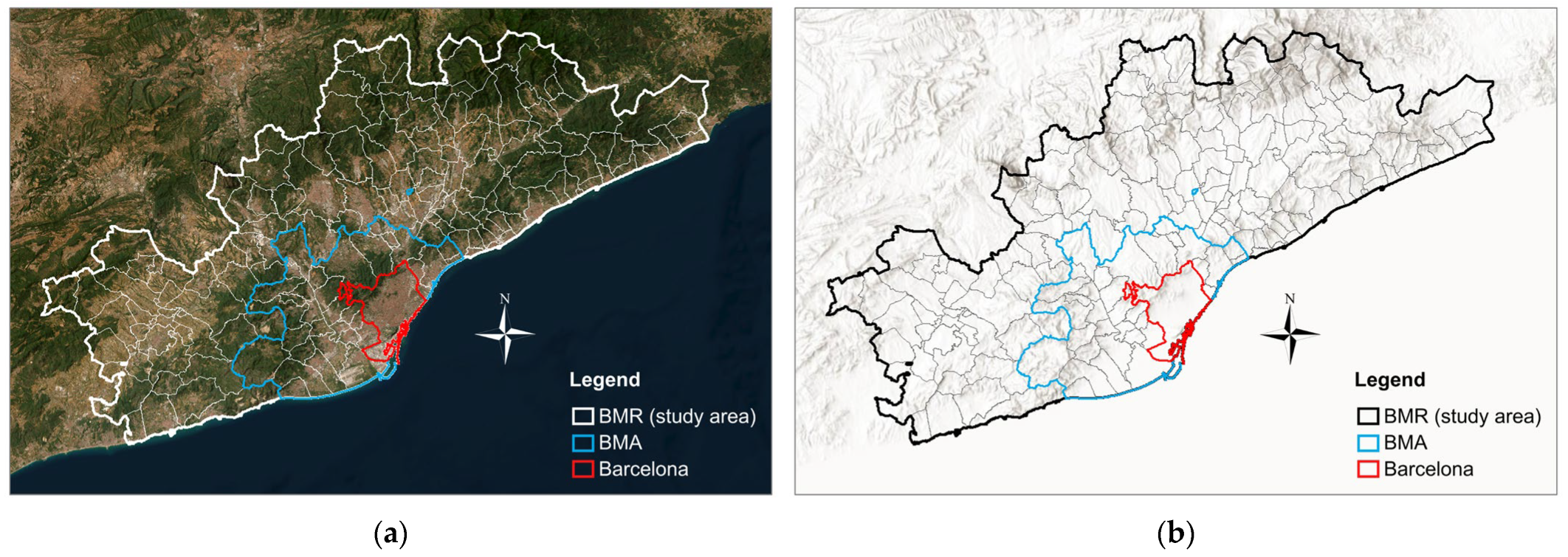
2.1. The Field of Study

The Barcelona Metropolitan Region (BMR, Figure 1) is located in the northeast of the Iberian Peninsula, at the heart of the Mediterranean corridor that connects Spain to the rest of continental Europe. It features a typical Mediterranean climate and is the largest metropolitan area in Catalonia, serving as its political, economic, and cultural center. Covering approximately 3224.7 km2 and comprising 164 municipalities, the BMR is home to about 5.4 million inhabitants, making it the most densely populated metropolitan area in the European Union [36]. The region is traversed by two major rivers, the Llobregat and Besòs, while the coastal and pre-coastal mountain ranges frame the coastal and pre-coastal depressions where most population centers are located. The Barcelona Metropolitan Area (BMA), a subset of the BMR, spans 636 km2 and includes the city of Barcelona and 35 neighboring towns, with a permanent population of roughly 4.7 million. The urban core of Barcelona, covering about 100 km2, has a population exceeding 1.65 million and a population density of over 16,500 inhabitants per km2 [37]. At the center of the metropolitan area lies the Collserola “serralada”, a key segment of the coastal mountain range that serves as the “green lung” for the region, providing a natural buffer amidst urban development. Recognizing the ecological significance of such green spaces, the Barcelona Metropolitan Territorial Plan prioritizes the protection of the BMR’s ecological environment and green infrastructure [38]. Currently, green spaces, including urban parks, suburban parks, forests, and protected areas, account for approximately 2514 km2, or 77.4%, of the total area of the BMR. Given these characteristics, the BMR was selected as the study area to assess the evolution of its ecological environment quality and to analyze the influence of various factors, particularly precipitation, on NDVI.

2.2. Materials

  • Corine Land Cover (CLC) provides us with relatively accurate European land cover data [39] with a resolution of 100 m in 2006, 2012, and 2018 (https://land.copernicus.eu/en/products/corine-land-cover, accessed on 18 June 2024), which records 22 types of green space systems in detail.
  • The MODIS_MOD13Q1 (https://lpdaac.usgs.gov/products/mod13q1v006/, accessed on 20 June 2024) dataset provides relevant remote sensing image data with a resolution of 250 m.
  • The daytime and nighttime land surface temperature (LST) can be obtained from MODIS_MOD11A1 (https://lpdaac.usgs.gov/products/mod11a1v006/, accessed on 20 June 2024) with a resolution of 1 km.
  • The urban heat island effect (UHI) will be expressed as the difference between urban and rural LST, that is, the difference in the average surface temperature between the urban built-up area and the rural area based on land cover data [40]. By subtracting the average surface temperature during the day and night in urban areas from that in rural areas each year, we can get the approximate intensity distribution of the urban heat island effect during the day and the night. The larger the value, the greater the intensity of the urban heat island effect.
  • DEM terrain data come from SRTM (https://www.earthdata.nasa.gov/sensors/srtm, accessed on 11 June 2024), with a resolution of 30 m.
  • Impervious ground data come from GlobeLand 30 (https://www.webmap.cn/commres.do?method=globeIndex, accessed on 15 June 2024), with a resolution of 30 m.
  • E-obs can provide annual European precipitation grid data, as well as daily maximum temperature (T_max) and minimum temperature (T_min), but the resolution is 1°, which is very large (https://surfobs.climate.copernicus.eu/dataaccess/access_eobs.php, accessed on 19 June 2024). Therefore, we used the kriging interpolation method based on the E-obs data to reconstruct the relevant climate map of the BMR with a resolution of 1 km [41].
  • The night light data are divided into two parts. The data from 1992 to 2013 come from DMSP data with a resolution of 30 arc seconds and a numerical range of 0–63. The night light data after 2013 are provided by VIIRS with a resolution of 15 arc seconds, which is more accurate and very different from DMSP. In the previous work of the authors, the two datasets were calibrated and unified using the stepwise calibration method, which will not be repeated here [42].
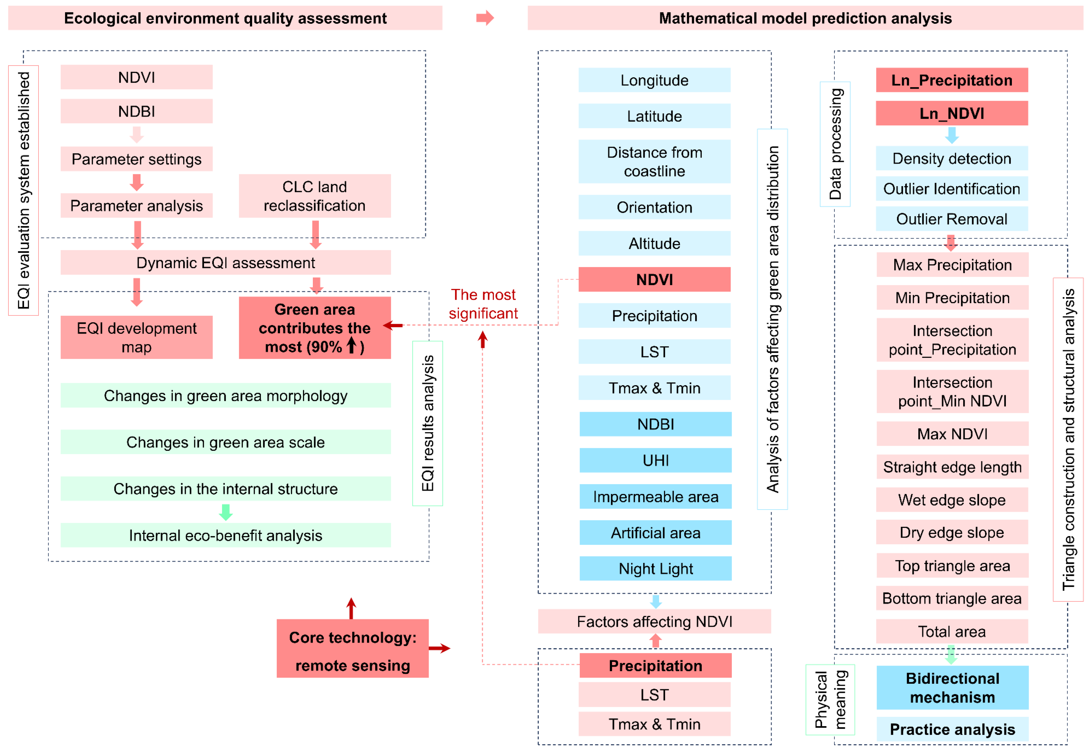
2.3. Methodology

We carried out this research in the following steps.
1
First of all, to evaluate the Ecological Environment Quality Index (EQI) of the BMR, we needed to achieve the following aspects.
  • For the convenience of analysis, we classified the land-use coverage of the BMR according to the land type classification of CLC [16].
  • Then, we extracted the difference (NDVIaverage-NDBIaverage) of the annual average values of NDVI and NDBI for each type of land in 2006, 2012, and 2018 after reclassification.
  • Secondly, set the EQI evaluation parameters. For each year, we homogenized the difference results obtained in the previous step using Formula (1), setting the minimum value of each year to 0 and the maximum value to 1 as the evaluation parameter (Ei) of ecological environmental quality.
E i = X 0 X m i n X m a x X m i n ,
where:
Ei is the dimensionless ecological environment quality weight index;
X0 is the NDVIaverage-NDBIaverage of each type of land in that year;
Xmax is the maximum value of NDVIaverage-NDBIaverage of various types of land in that year;
and Xmin is the minimum value of NDVIaverage-NDBIaverage of various types of land in that year.
  • Finally, I evaluated the BMR’s annual EQI index based on Formula (2).
E Q I t = i = 1 n A i × E i T A ,
where:
EQIt is the ecological environment quality index in year t;
i is the land type;
Ai is the area of that type of land use;
Ei is the weight of the ecological quality index of this type of land use;
and TA is the total area of the land.
  • It is important to pay attention to the land-use types that have a greater impact on or contribution to the evaluation results when evaluating the ecological environment quality of urban areas. Land use is the key to controlling the ecological quality of the BMR.
  • In addition, we also needed to draw the distribution map of the annual evaluation results of the ecological environment quality index of the BMR and the change map of the results from 2006 to 2018 to analyze the distribution and evolution direction of the ecological quality of the BMR from a spatial perspective.
2
Then, we needed to study the relationship between the key land-use distribution and various possible influencing factors that affect the assessment results. We have reviewed numerous relevant studies and compiled various data on green space distribution, which are presented in Table 1 [5,43,44]. After obtaining the above data, we established a 1km grid within the BMR range, extracted the proportion of key land-use area in the grid each year as the dependent variable, and established an OLS model to analyze their importance.
3
Having established a clear interaction between NDVI and the distribution of key land uses that influence EQI assessment results, it is necessary to analyze the climatic factors affecting NDVI to uncover the indirect impacts of climate change on ecological quality. For this purpose, a climate database spanning 2000 to 2023 was developed, with the annual average NDVI as the dependent variable and multiple climate data as explanatory variables. The strength of the correlations between these variables was then analyzed.
4
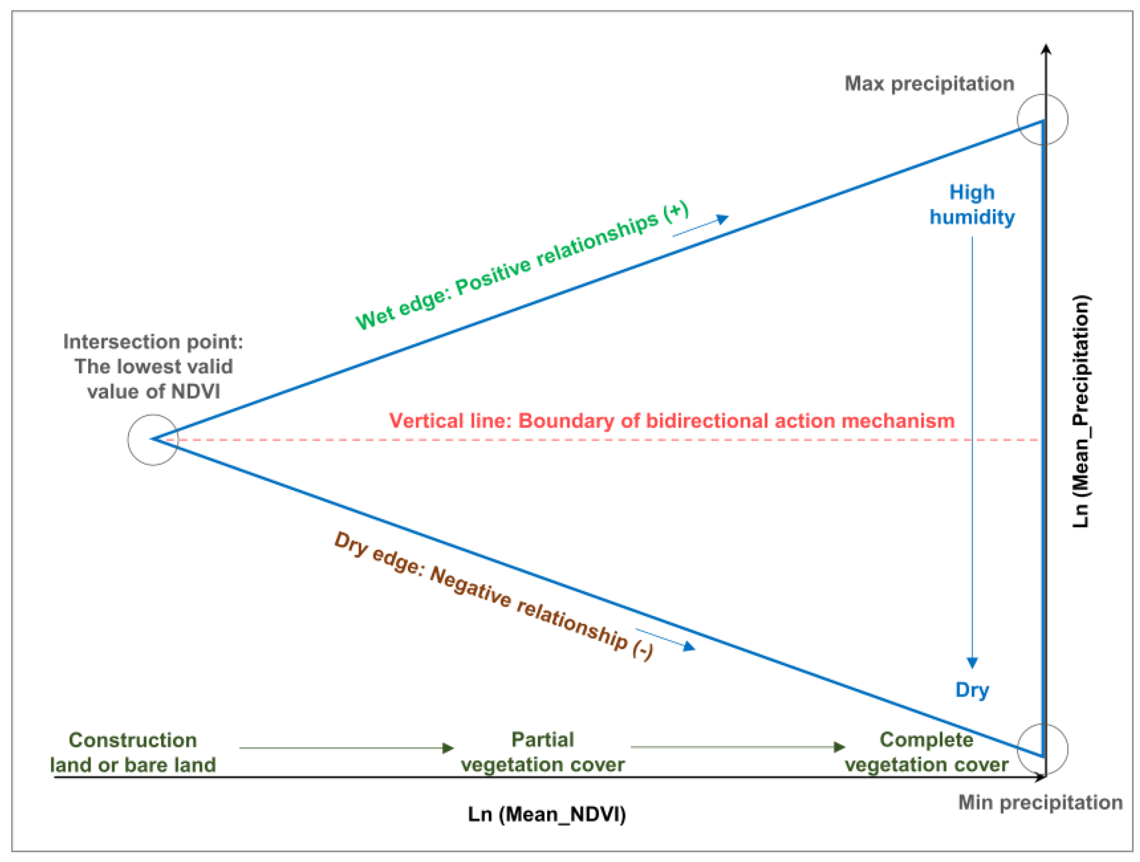
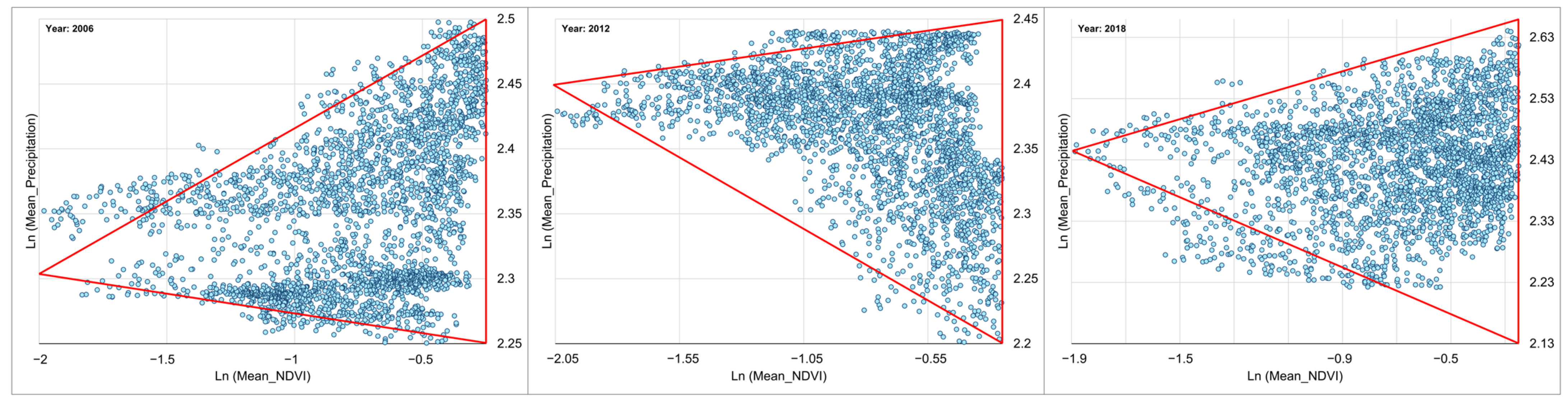
In a previous study, the authors identified precipitation as a highly complex controlling factor [25], with a strong, yet unresolved, interaction with NDVI. However, this intricate relationship proves challenging to elucidate using conventional regression models [45]. To address this, we employed the precipitation/NDVI characteristic triangle space as an analytical framework to explore the underlying mechanism [46,47,48].
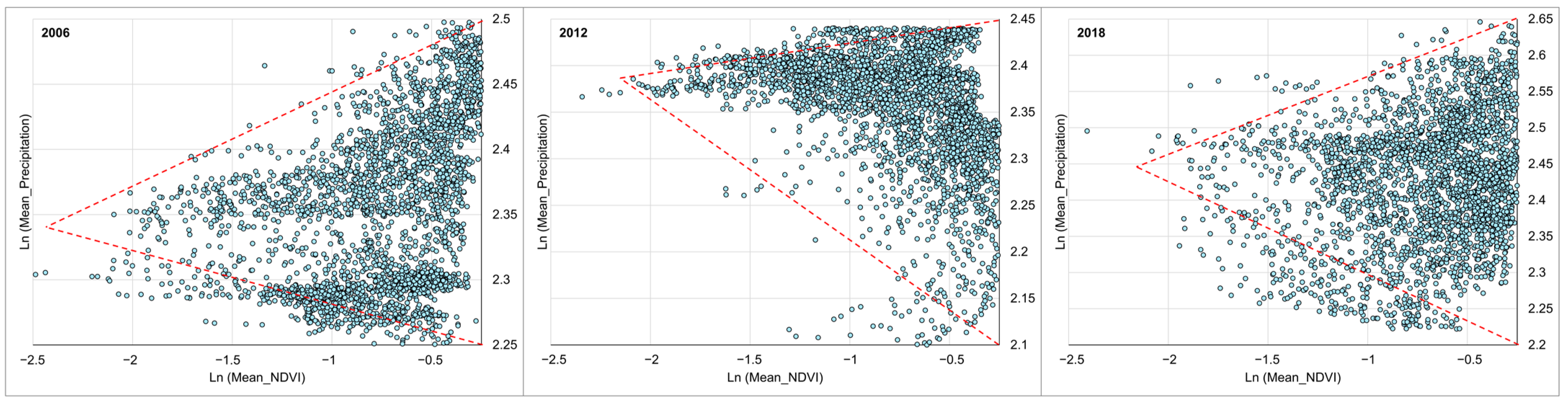
  • Firstly, for each year, a precipitation/NDVI scatter plot was established. In order to facilitate the analysis of the physical meaning of each side of the triangle, we used NDVI as the X-axis and precipitation as the Y-axis. Since the numerical ranges of the two values are quite different, the spatial characteristics of the established scatter plot are not obvious, so we calculated the Ln log function for both NDVI and precipitation [49].
  • Then, Qrigin 2021 was used to perform nonparametric kernel-density estimation (KDE) to analyze the density characteristics of the scatter plot [50,51,52].
  • If it is found that the scattered points are unevenly distributed and there are scattered points with low density distribution around the cluster, we need to perform local outlier factor detection (LOF) [53,54].
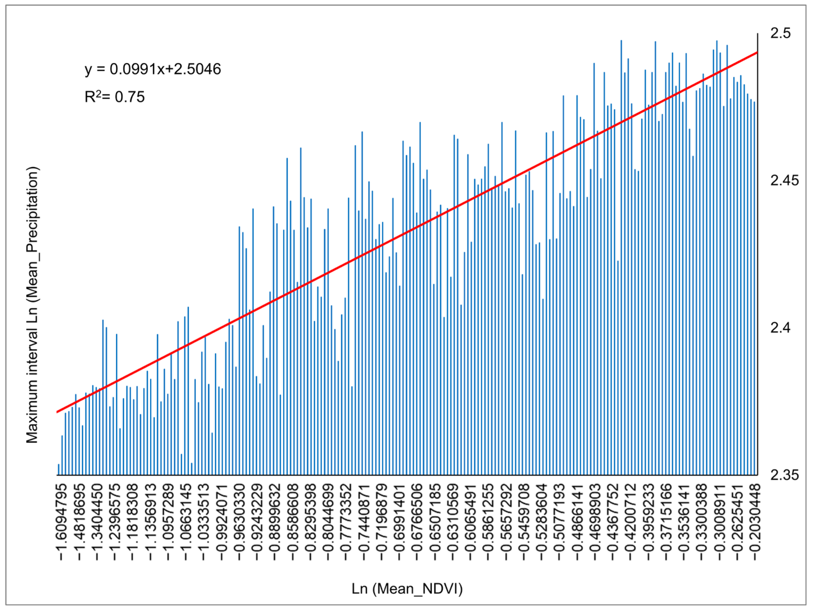
  • After removing the abnormal outliers, we can determine the sides of the characteristic triangle. The maximum NDVI value among the retained scattered points will be used as the straight edge. For the hypotenuse, we use 0.01 as a minimum interval and find the maximum and minimum precipitation values in each interval. Then, use the least squares method to perform a linear fit with Equation (3) to obtain the hypotenuse of the triangle [46].
P r e c p i = a   ×   N D V I i
where:
Precpi is the LN value of precipitation corresponding to the i-th NDVI;
NDVIi is the LN value of NDVI corresponding to the i-th NDVI;
a is the slope;
and b is a constant.
  • Finally, after completing the most critical triangle fitting, we can use remote sensing technology to analyze the physical meaning of each side of the precipitation/NDVI characteristic triangle and the space and further analyze the relationship between NDVI and precipitation. This allows us to indirectly understand the impact of precipitation on the green space system.
The research method is summarized in the following idea map (Figure 2).

3. Results

3.1. BMR Ecological Environment Quality Assessment

Extensive research has been conducted on ecological environment quality assessment using remote sensing technology, producing significant results from various perspectives and focuses. Initially, studies primarily employed environmental indicators to assign numerical weights based on land cover types for assessing the environmental quality of specific regions [8,11,12,13,14,15,16,17,18,19,20,21]. While these assessments have evolved from relying on single indicators to multiple indicators with increasingly refined land-use classifications and improved weight assignments, their applicability remains limited to specific areas and timeframes. Due to the complexity and variability of natural environments, this method poses challenges for long-term comparisons across diverse regions. In recent years, growing attention has been directed toward the spatiotemporal evolution of ecological environments, leading to the development of new comprehensive assessment methods [22,23,24]. However, these methods often involve complex parameter settings, require extensive datasets, and lack sufficient analysis of ecosystem processes, dynamics, and functionality.
The Normalized Difference Vegetation Index (NDVI) is a widely used indicator in vegetation remote sensing research for detecting plant biomass, vegetation coverage, and growth status. It is considered the most effective index for assessing regional ecological vulnerability [55,56,57]. Vegetation plays a crucial role in terrestrial ecosystems, serving as a key medium for the material and energy cycles of the Earth’s ecosystem [58]. NDVI changes provide valuable insights into regional ecological evolution [59]. High NDVI values typically indicate dense vegetation, which reflects favorable humidity and temperature levels, enhancing ecosystem resilience and biodiversity [31]. In a previous study, the authors observed that tall tree canopies in summer might lead to overestimated NDVI values, whereas in winter, long-wave radiation from the ground is less affected by the tree canopy [60]. Therefore, this study seeks to establish ecological quality weights for different land uses by analyzing NDVI in both summer and winter. The Normalized Difference Built-up Index (NDBI) is another critical remote sensing indicator for evaluating ecological environment quality [61,62]. It reflects the extent of urbanization’s interference and damage to ecosystems [63]. High NDBI values diminish the ecological function of vegetation [64], exacerbate local microclimatic conditions [65], and highlight the negative impacts of human activities on ecological environments [66]. Subtracting NDBI from NDVI provides a more accurate representation of a region’s ecological effects.
To address the limitations mentioned above, and based on an analysis of the two most important indicators, NDVI and NDBI, this study adopts the dynamic land-use weight index method proposed by Hou Yifeng et al. [16]. This approach estimates the ecological environment quality index of the Barcelona Metropolitan Region (BMR) by assigning weights that dynamically adjust according to changes in land cover within the study area. The method is highly adaptable to specific contexts under a consistent land-cover classification standard, allowing for comparisons across different study objects. It not only addresses the shortcomings of fixed-parameter evaluations but also supports the analysis of long-term ecosystem dynamics. Additionally, it enables the evaluation of the ecological contributions of various land types.

3.1.1. Green Area Is the Key Land Use That Provides Ecological Benefits

To establish the proposed ecological quality-assessment system, we first reclassified the land-use types in the BMR based on the CLC’s land-cover classification framework [67]. Additionally, to more intuitively identify key land types that provide significant ecological benefits, the 11 subdivided land categories were consolidated into five main classes (Table 2).
The evaluation parameters of ecological environment quality for each land-use type during different periods directly reflect the contribution of land use to the local ecological environment. Analyzing these changes provides insights into the evolution of ecological benefits associated with land use. Figure 3a illustrates the ecological quality parameters of various land-use types in the BMR from 2006 to 2018.
The most notable contributor is forest land, which consistently provides the highest ecological benefits, maintaining a parameter value of 1 across all periods. Grassland ranks second, with parameters remaining above 8.2 throughout the three years. However, the land-use type contributing the least to the ecological environment varies by year. In 2006, continuous urban land had an ecological parameter of 0, but this value sharply increased to 0.22 the following year, while wasteland, which had previously performed better, became the lowest contributor. By 2018, the ecological benefits of wasteland recovered rapidly, while industrial land saw a significant decline, with its parameter dropping from 0.3 to 0.
Water bodies showed relative stability in the first two years, with parameters exceeding 0.4, but their values more than halved in 2018. Land-use types with lower ecological benefits exhibited greater fluctuations over the three periods. Overall, ecological parameters peaked in 2012 and were generally lower in 2018 compared to the other two years. Notable exceptions include transportation land and water bodies, which performed worse in 2012 than in other years, and grassland, which achieved higher parameters in 2018 compared to 2006.
Figure 3b illustrates the changes in the ecological and environmental parameters of the main land-use categories in the BMR and the overall trends over time. Notably, the green area provides the highest ecological benefits, far surpassing other categories. In 2012, the parameter for green areas peaked at approximately 3.33, while in 2018, it recorded the lowest value at just above 2.9, still maintaining its leading position.
Construction land ranks second, with its parameter reaching a maximum of about 0.95 in 2018. Urban land, on the other hand, exhibited the most unexpected trend; starting at only 0.1 in the first year, it soared to 0.43 before rapidly declining to 0.19. Overall, the ecological benefits of all land categories were highest in 2012, totaling 5.15, and lowest in 2018, at just 3.79.
The parameter evolution of most land-use categories aligns with this general trend, except for wasteland, which deviates from the overall pattern.

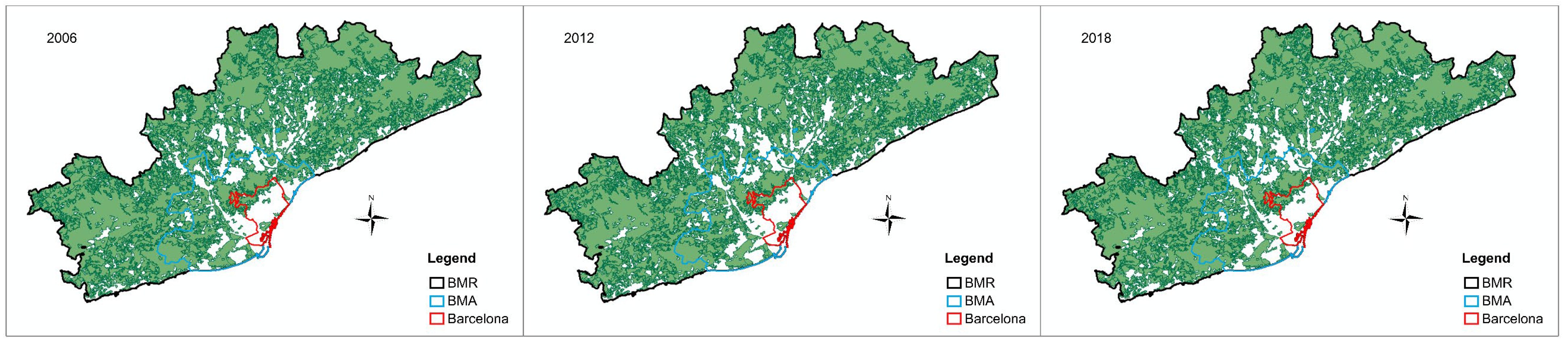
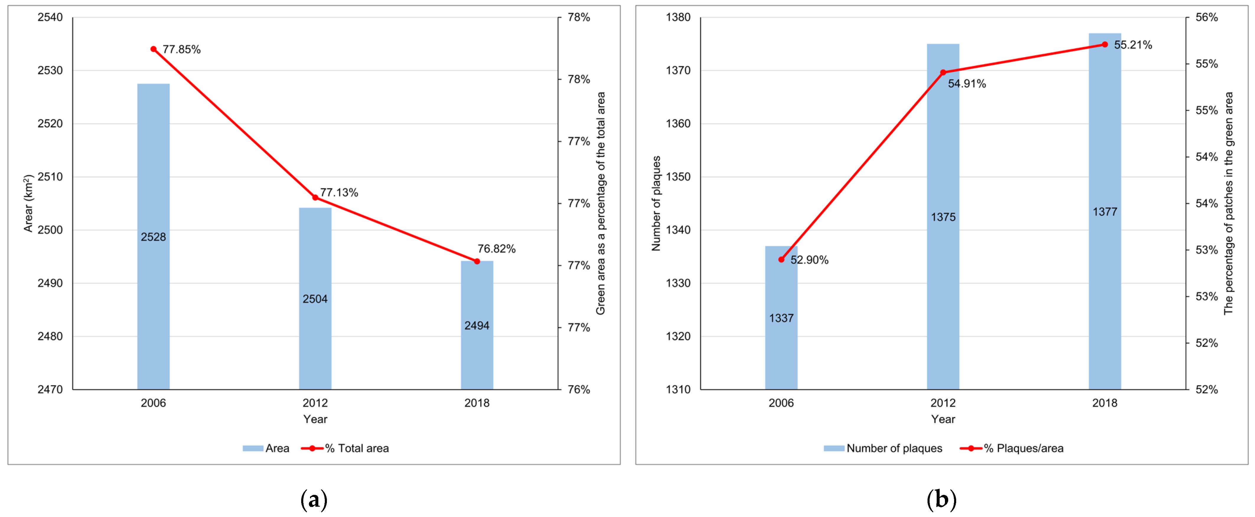
3.1.2. The Green Area Is Shrinking but Becoming More Fragmented

Analyzing the development process of land-use distribution that most benefits ecological and environmental protection is crucial for understanding the factors driving changes in ecological quality and guiding the direction of environmental conservation efforts. Figure 4 conveys a positive message; between 2006 and 2018, green areas dominated land use in the BMR, with land providing the highest ecological benefits becoming the predominant land-use type in the metropolitan region. Large green areas are concentrated in the northern, eastern, and southwestern parts of the BMR, while the central urban area has relatively sparse green coverage.
Figure 5 illustrates the evolution of the area and number of green area plaques in the BMR. It is clear that while the total area of green space continues to decrease, the number of plaques gradually increases. In 2006, the green area of the BMR covered 2528 km2, accounting for more than 77.8% of the total area. After 12 years of decline, it decreased by approximately 33.3 km2, though the overall situation remains satisfactory. By the last year, more than 76.8% of the land in the BMR remained as green space, despite the reduction. However, the fragmentation of green areas has become more pronounced, increasing from 1337 plaques in 2006 to 1377 plaques in the most recent year. The density of plaques also rose from 52.9% to 55.2%. While the area has reduced, the fragmentation has increased, indicating that the spatial distribution of green areas in the BMR has become more complex. This could be detrimental to ecological environmental protection.

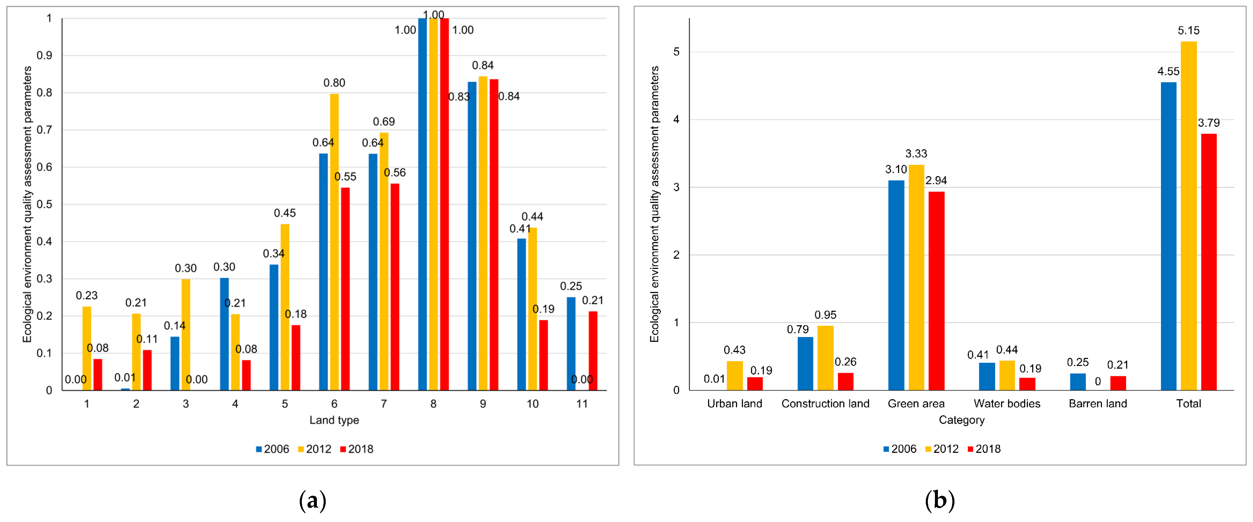
3.1.3. The Ecological Quality Results of the BMR Are Generally Appreciable, with Green Area Making the Largest Contribution

After establishing the ecological environment quality-assessment system for the metropolitan region, we obtained the overall assessment results for each land type and for the BMR (Table 3). Overall, the ecological quality results for the BMR during the study period are impressive, with values consistently above 0.67. Notably, in 2012, the score reached 0.74, the only instance during these three years when it exceeded 0.7. The assessment results for 2018 were slightly lower than those of 2006, but only by 0.02.
Among all land categories, as expected, the EQI results for green areas, which provide the highest ecological benefits, are also the highest, almost determining the overall ecological quality of the BMR. In 2006 and 2018, the EQI of green areas was 0.68 and 0.65, respectively, accounting for over 97% of the total results. In 2012, the year with the highest EQI for green areas, its contribution to the overall BMR results dropped to around 92.8%, although this value remains much higher than that of other land types. In other years, urban land, which has always accounted for a small proportion, became the second largest contributor in 2012, accounting for approximately 4.2% of the total results. The proportion of construction land in the total results is relatively significant compared to the other two land types. The ecological contribution of water bodies has been decreasing, and the EQI of wasteland remains the lowest among all categories. The specific EQI evaluation results for various land types are detailed in Appendix B.

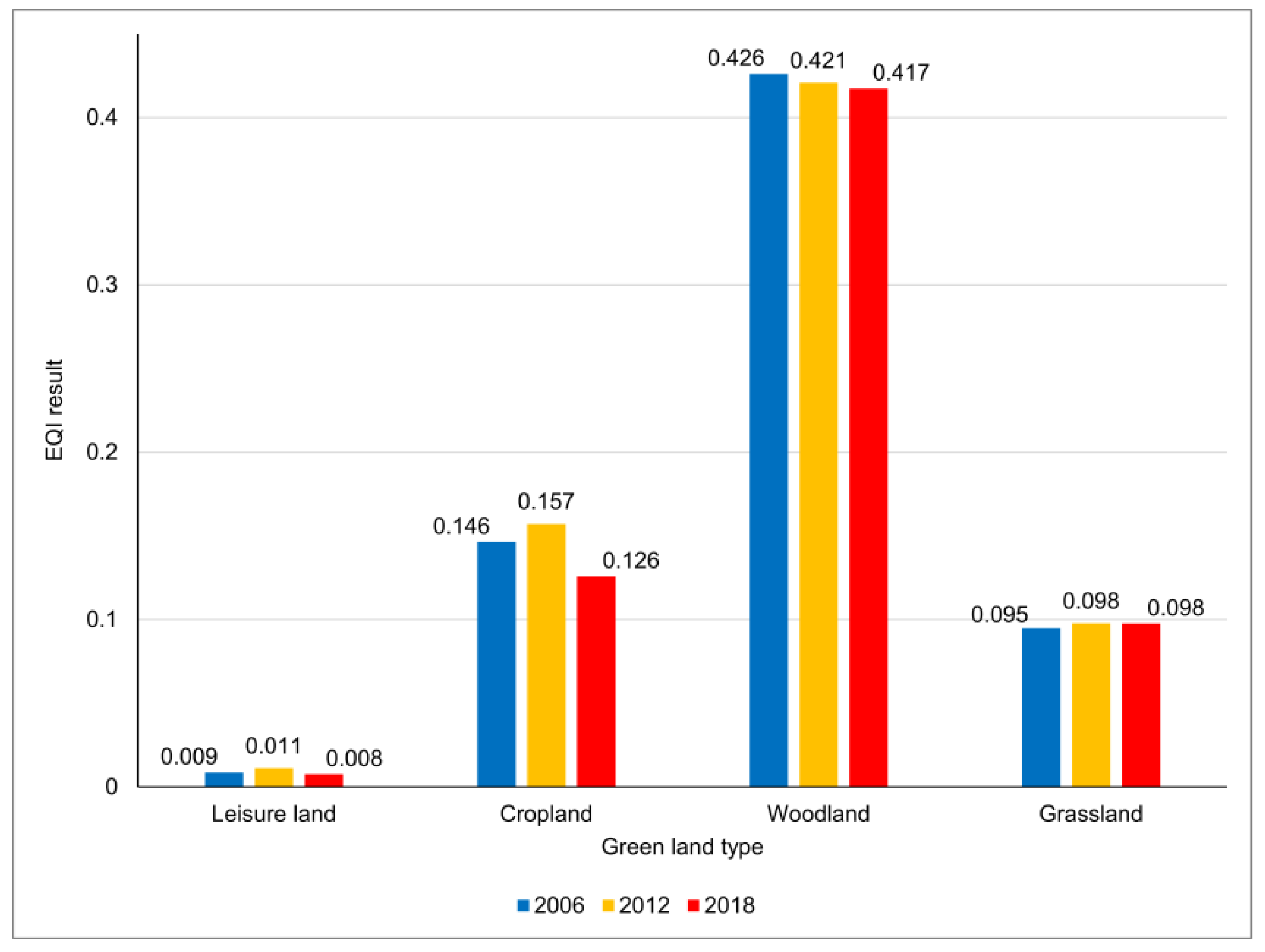
3.1.4. The EQI of Forests Cannot Be Ignored

Green areas contribute the most to the EQI assessment results and are the decisive factor in determining the ecological quality of the BMR. Therefore, analyzing the EQI of various land types within green areas is essential. Figure 6 presents the EQI assessment results for different types of green land in the BMR from 2006 to 2018. It is evident that forests have made the most significant contributions. Throughout the three years, the EQI for forests consistently ranked highest, although it showed a slight decline, decreasing from 0.426 to 0.417.
Farmland ranked second, with its EQI increasing from 0.146 to 0.157 in 2012, reaching a peak, but then dropping to 0.126 in 2018. Grassland exhibited relatively stable performance, remaining around 0.1 during the study period with a slight upward trend. The lowest EQI was observed in recreational land, which refers to green spaces within the city. The EQI for recreational land was consistently around 0.01 throughout the three years, reaching a low point in 2018.

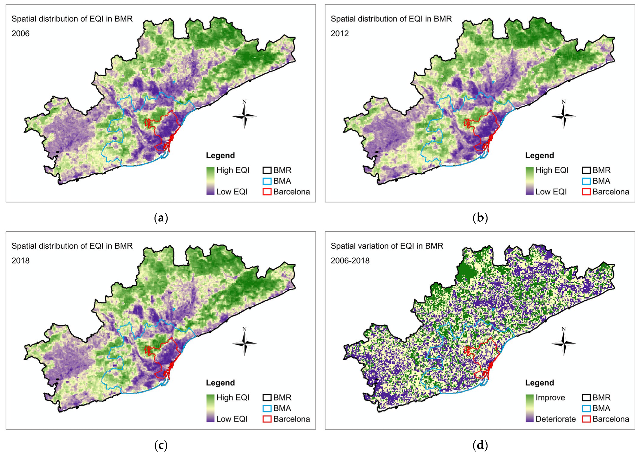
3.1.5. BMR Ecological Environment Quality Distribution Needs to Be Improved

The spatial distribution map of EQI assessment results helps analyze the environmental quality distribution across the BMR and identify areas with good ecological conditions as well as those in urgent need of improvement. As shown in Figure 7a–c, despite the large green areas with high ecological parameters in the BMR, nearly half of the land exhibits low EQI values across all three years. The core area of Barcelona presents the most concerning situation, with only a small portion in the north showing good ecological quality, while the rest of the area has very low EQI values.
The ecological situation in the Barcelona Metropolitan Area (BMA) is slightly better than that of Barcelona, but it still consists mostly of areas with poor ecological quality. Small areas in the west, north, and northeast of BMA show good ecological results. In the BMR as a whole, the coastal areas, large portions in the east, and continuous stretches in the north have very poor ecological quality, especially around Barcelona and its surrounding areas. While the northern and eastern regions of the BMR exhibit very high EQI values, the high assessment results are scattered across the north, central south, and northwest regions.
To provide a more intuitive analysis of the evolution of the BMR’s EQI from 2006 to 2018, we created a map illustrating changes in ecological environment quality (d). The map reveals that most of the BMR’s ecological quality has either remained unchanged or improved. Barcelona remains the most unsatisfactory area, with much of it experiencing deterioration or no change, and only a few areas showing improvement. In the BMA, ecological quality deterioration is mostly concentrated in the southwest, while significant improvements have been observed in the northern and eastern areas. The western end, south-central, north-central, and northeastern parts of the BMR are areas where ecological quality deterioration is more concentrated. The northern region stands out, with significant improvements in EQI. The remaining areas are primarily characterized by improvements or no change.

3.2. Analysis of Factors Affecting Green Area Distribution

To explore the influence of various factors on the distribution of green areas, which play a critical role in controlling EQI results, we established a grid with a side length of 1 km. The area ratio of green spaces in each grid was set as the dependent variable, with independent variables including longitude, latitude, distance from the sea, aspect, altitude, slope, average NDVI for winter and summer, annual precipitation, daytime and nighttime Land Surface Temperature (LST), the difference between daytime and nighttime LST, maximum temperature (T_max), minimum temperature (T_min), the temperature difference (T_max-T_min), NDBI, daytime and nighttime urban heat island effect, impervious surfaces, and artificial land. Three ordinary least squares (OLS) regression models were developed for the years 2006, 2012, and 2018 (Table 4), with over 10 significant variables, achieving an R2 value of 0.97.
Among the natural factors, the most significant influence on the distribution of green areas is NDVI (+), although its explanatory power has gradually weakened. Following this is annual precipitation (+), the difference between maximum and minimum temperatures (−), and maximum temperature (+), with the latter two showing a sudden increase in influence, especially in the last year. The difference between daytime and nighttime surface temperature (+) also plays a significant role.
From the perspective of human activities, artificial ground (−) and impervious surfaces (−) are the primary barriers controlling the distribution of green areas, followed by NDBI (−) and the urban heat island effect at night (−).
It is undisputed that artificial surfaces and impervious areas are the most fundamental factors controlling the distribution of green areas. The model results indicate that these two factors alone can explain approximately 90% of the variation in the distribution of green areas within the BMR. However, in comparison to human-induced activities, analyzing uncontrollable natural factors is more meaningful in this study. In 2012 and 2016, the average NDVI explained more than 54% and 67% of the variation in green areas, respectively, when considering only natural factors. However, by 2018, its explanatory power had decreased to 35% due to the increasing significance of the difference between maximum and minimum temperatures and the maximum temperature.
When NDVI, artificial surfaces, and impervious areas are considered together, their combined influence on green areas exceeds 90%. The reason why diurnal LST, minimum temperature, and the daytime urban heat island effect were not included in the optimal model is due to their high collinearity with the difference between diurnal LST, maximum temperature, and the difference between maximum and minimum temperatures. The relevant Pearson correlation coefficients in the model are presented in Appendix C.

3.3. Analysis of Climate Factors Affecting NDVI Evolution

There is a significant interaction between the average NDVI and the distribution of green areas, which plays a key role in controlling ecological environment quality. More importantly, it is essential to examine the climate factors most closely related to the development of NDVI and explore the indirect impact of climate change on the ecological environment quality of the metropolitan region. To achieve this, we used the annual average NDVI from 2000 to 2023 as the dependent variable and established five OLS models with annual precipitation, maximum and minimum temperatures, and daytime and nighttime surface temperatures as independent variables. These models were used to analyze the linear relationship between climate factors and NDVI change trends. Table 5 presents the detailed results of all model analyses.
The most significant positive correlation with the mean NDVI is precipitation (sig. < 0.001), with the R2 of the regression model between them reaching 0.47, the highest fit among the five models. Precipitation alone explains approximately 50% of the annual evolution of NDVI. Following this, minimum temperature (−) and daytime LST (−) also influence NDVI changes, although their explanatory power is much weaker than that of precipitation. Variables with almost no effect include nighttime LST (t = 0.62) and maximum temperature (t = 0.25). The Pearson correlation coefficients for the relevant variables in all models are shown in Appendix D.
Figure 8 illustrates the evolution of the annual average NDVI and the statistical averages of five related climate factors in the metropolitan region from 2000 to 2023. To facilitate direct observation and comparison of their change patterns, we normalized the values of all variables, ensuring that their annual statistical values fall within the range of 0−1. It is evident that the change pattern of annual precipitation most closely mirrors that of the average NDVI, with both showing similar periods of increase and decrease. Although there were some deviations in 2001, 2009, and 2016, the overall trends closely align.
Before 2020, both the annual NDVI and precipitation in the BMR exhibited a slow, fluctuating growth trend, after which they dropped rapidly, reaching their lowest values in recent years in 2023. While the change patterns of several other temperature-related variables are not as closely aligned with NDVI as precipitation, their growth trends have clearly accelerated in recent years, reaching a peak in 2022 due to the warming climate. In the specific research years selected, 2006, 2012, and 2018, the change patterns of NDVI and precipitation were relatively similar, with no unexpected anomalies. Therefore, this provides a solid database for analyzing the specific relationship between the two in the next step.

3.4. Spatial Analysis of Precipitation/NDVI Characteristic Triangle

3.4.1. Spatial Definition of Precipitation/NDVI Characteristic Triangle

Using scatter plots to analyze the correlation between variables, identify outliers, and perform trend fitting is a relatively basic reference and research tool [46]. Prior to this, scholars have established scatter plots using NDVI and other various climate factors, confirming that there is a relatively obvious and stable characteristic triangular spatial feature between NDVI and them. In the early days, scholars performed linear fitting on the double edges of the scatter distribution based on the scatter distribution characteristics between LST and NDVI and obtained the triangular spatial structure of LST/NDVI [47,48]. Later, it was proposed that there is a more stable single-hypotenuse triangle spatial feature between NDVI and night light intensity, which was verified in five cities around the world, and the physical characteristics of the three-sided structure of the triangle were used to successfully extract urban areas and classify cities in multiple cities [46]. By analyzing the scatter plot established by using the log function of Ln to process the precipitation and average NDVI in 2006, 2012, and 2018, we can see that there is also a similar double-hypotenuse triangle spatial structure feature between the two (Figure 9).
Inside the triangular space, each scatter point is represented by precipitation and NDVI, reflecting the degree of humid or dry climate conditions given varying levels of green vegetation coverage. The upper hypotenuse represents the positive correlation between precipitation and NDVI, while the lower hypotenuse reflects the negative relationship between the two variables. The vertical edge on the right represents areas with high vegetation coverage and high precipitation, while the intersection on the left represents the lowest effective NDVI threshold.
More importantly, the vertical line extending from the triangle’s vertex to the right side helps us understand the mechanism between precipitation and NDVI. Above the vertical line lies a humid area with abundant precipitation, which promotes vegetation growth. In contrast, below the vertical line, under relatively dry conditions, the slope of the equation line between vegetation cover and precipitation becomes negative, indicating an inverse relationship between the two. Figure 10 provides a more intuitive explanation of the composition and meaning of each part of the precipitation/NDVI triangular spatial feature.

3.4.2. Construction of the Triangular Spatial Structure of the Precipitation/NDVI Scatter Plot

Kernel-density estimation (KDE) is a nonparametric method used in probability theory to estimate the probability density function of an unknown random variable. Proposed by Rosenblatt [50] and Emanuel [51], KDE infers the overall data distribution based on a limited sample and analyzes the concentration of data points. Unlike parametric methods, it does not rely on the assumptions about the overall distribution and its parameters but derives the structural relationships directly from sample data [52].
We applied kernel-density estimation to analyze the distribution density of scatter points in three scatter plots of NDVI and precipitation in the metropolitan region for the years 2006, 2012, and 2018. The results are presented in Figure 11. It is evident that the scatter point distribution is highly uneven, with density decreasing from areas of high concentration to the surrounding regions. The red dotted box highlights several relatively clear low-density clusters. A large number of low-density scatter points at the edges of the triangle create gaps in the triangular spatial structure, failing to accurately reflect the precipitation and vegetation coverage of the metropolitan region. Therefore, these peripheral scatter points must be removed for a more accurate representation.
We performed local outlier factor (LOF) detection on all scatter points. This detection method is a density-based outlier detection algorithm that identifies outliers by calculating the outlier factor of a sample and comparing it to the density of surrounding data points [53]. Outliers typically appear isolated, and samples with larger LOF values exhibit lower density, classifying them as outliers. During the identification process, points are considered outliers when the ratio between their distribution density and the overall average density is significantly greater than 1 [54]. Figure 12 presents the results of abnormal outlier identification for scatter point density. The blue bubbles represent the LOF detection results for the scatter points. The larger the radius, the greater the possibility of being an outlier, and the red scattered point is the detected outlier that needs to be removed. This result is similar to the analysis in the previous step. A large number of free scattered points with low distribution density are selected, among which the highly concentrated scattered points in the core of the triangular structure are effectively retained. On this basis, we can construct the final precipitation/NDVI triangle structure.
The straight side of each characteristic triangle is derived by effectively retaining the maximum NDVI value, while the hypotenuse is fitted using the segment’s extreme values. We divide Ln (Mean_NDVI) into several small intervals, each with a width of 0.01. The upper and lower hypotenuses of the characteristic triangle are then determined by the maximum and minimum precipitation intensities that can be supported under the NDVI conditions for each interval. After identifying the precipitation extreme values and their corresponding NDVI for each interval, we apply the least squares method for linear fitting. As an example, we use the maximum annual precipitation in 2006 and the upper hypotenuse of the triangle to illustrate the fitting method for the hypotenuse (Figure 13).
The characteristic triangular spatial structure of the scattered point distribution of the three years and the fitting results of each side are finally presented in Figure 14 and Table 6.

3.4.3. Analysis of the Physical Meaning of the Triangular Space of the Precipitation/NDVI Scatter Plot

  • Analysis of parameters of spatial structure of precipitation/NDVI characteristic triangle
Table 7 summarizes the parameters of all characteristic triangle structures, providing an intuitive representation of the dynamic changes in the multiple interactions between precipitation and NDVI over the years. Between 2006 and 2018, the maximum precipitation in the metropolitan region initially decreased slightly before increasing, with the final value of 14 mm surpassing the initial 12 mm. Meanwhile, the minimum precipitation continued to decrease. The length of the straight edge indicates the threshold of the average annual precipitation. It is evident that the thresholds in 2006 and 2012 were not significantly different, with a decrease of about 0.02, followed by an increase to 0.48, which is more than twice the value of 2012.
The precipitation at the intersection represents the boundary of the relationship between precipitation and NDVI. Above this point, there is a positive cooperative relationship between the two variables, while below it, they exhibit mutual inhibition in an opposite direction. This critical value clearly increased over time, from 10.05 in 2006 to 11.51 in 2018. This suggests that, over time, precipitation must increase to significantly and effectively promote the growth of green vegetation on the surface.
The NDVI at the intersection represents the minimum effective NDVI in the characteristic triangle space. The values across the three years were not significantly different, remaining around 0.14. The straight side of the triangle represents the maximum NDVI, marking the endpoint of the effective interaction between precipitation and NDVI. The maximum NDVI in 2006 and 2018 were similar, around 0.83 and 0.85, respectively, while the minimum value in 2012 was about 0.79. The closer the points are to the straight edge, the more scattered they become, indicating a more complex relationship between precipitation and NDVI.
The strength of the relationship between precipitation and NDVI can be assessed by the slope of the hypotenuse. In 2006, the slope of the wet edge (0.1) was much steeper than that of the dry edge (0.03), indicating that in that year, precipitation primarily promoted NDVI growth. In contrast, the dominant mechanism in 2012 was mutual inhibition, where higher precipitation did not effectively promote vegetation growth. The distribution of high precipitation areas covered by higher vegetation was smaller than that of low precipitation areas, and even the average precipitation in these areas was less favorable compared to more exposed surfaces. In 2018, the slope of the top hypotenuse was 0.11, while the slope of the bottom hypotenuse increased slightly to 0.16. However, from the scatter distribution, there was a small blank in the bottom corner of the triangle in 2018, so from the overall consideration, the average precipitation in the area of high NDVI was greater than the model-estimated results. In the last year, the positive effect between the two may be more significant than the negative effect, or the two relationships are in a dynamic equilibrium mode.
The area of the triangle further reinforces the strength and complexity of the two interaction relationships. We divided the precipitation/NDVI characteristic triangle into two parts, the upper and lower triangles, with the vertical line acting as the dividing line. The upper triangle represents the promoting effect of precipitation on NDVI, while the lower triangle represents the reverse effect. As mentioned earlier, the coexistence pattern of precipitation and NDVI in 2006 was significantly stronger than the mutual interference, whereas the opposite was true in 2012. The area of the triangle in the dominant state during these two years was much larger than the other.
In 2018, the areas of the two triangles were similar. However, considering the blank space in the lower triangle in 2018, the areas of the two triangles would be closer, or even the wet hypotenuse could be wider. Additionally, the larger the area of the triangle, the more scattered points it contains, which implies a more complex interaction mechanism between precipitation and NDVI. Overall, the areas of the characteristic triangles in 2006 and 2012 were similar, with almost negligible reduction. In contrast, in 2018, the area of the triangle surged to 0.41, more than twice the size of the previous years. The interaction relationship in 2018 was the most complex.
  • Practical analysis of spatial structure of precipitation/NDVI characteristic triangle
To understand the actual meaning of each edge of the precipitation/NDVI characteristic triangle structure in the metropolitan region and the spatial distribution pattern of the scattered points near them, we selected the three edges of the characteristic triangle and the scattered points near the vertical line from the vertex to the straight edge as samples with a width of 0.01 units. We then restored the actual pixel positions of these scattered points on the BMR map and created Figure 15. Additionally, we integrated the physical significance of each edge with the EQI results for each land-cover type in the metropolitan region, as previously evaluated. This approach provides the opportunity to summarize the relationship between the precipitation/NDVI characteristic triangle and ecological quality.
In 2006, the top edge of the characteristic triangle, where scatter points with high precipitation are predominantly found, was located in forests, cultivated land, and grasslands in the northern part of the BMR, areas that also exhibit very high environmental quality. Additionally, a small number of urban and built-up lands with poor ecological quality were scattered in some places in the northern part of the central BMR. The NDVI in these locations increases with precipitation. On the bottom edge, the NDVI is inversely proportional to precipitation, and the scatter points were concentrated in cultivated land and forests in the southern BMR. A few were also found in the central BMR, particularly in the BMA and Barcelona, which have a high level of human development. Compared to the top edge, nearly half of the scatter points on the bottom edge were located in urban and built-up land areas, where the NDVI is inversely related to precipitation. Overall, the EQI of pixels near the bottom edge of the triangle is lower than those near the top edge.
In contrast, in 2012, the locations of the pixels near the two hypotenuses of the triangle shifted. The southern part of the metropolitan region became the main distribution area for scatter points near the wet edge, with a few pixels also appearing in the northern and central parts of the BMR. These pixels still tended to be located in green areas with higher EQI, though exceptions appeared in the BMA, where urban land with a lower environmental quality index had a considerable number of top pixels. Many dry edge pixels were found in forested areas in the northern part of the metropolitan region, along the coastline, and in the central and surrounding areas. These pixels were distributed not only in green areas with high EQI but also in urban and built-up lands with lower EQI. However, overall, there was no significant difference in ecological quality between the pixels near the top and bottom edges in 2012. During this period, precipitation was more abundant in the southern BMR, and the lush vegetation cover resulted in higher NDVI values.
In 2018, the top edge pixels were located in the northern and southern parts of the BMR, with forests and cultivated lands being much more prevalent than urban or built-up areas. These scatter points were also retained in the eastern and northern parts of the BMA. Dry edge pixels appeared in the north-central, central, and southern coastal areas of the BMR, predominantly on artificial surfaces with low ecological quality, although a few were concentrated in forested areas in the northernmost part.
The scatter points near the straight edge in all three years had very high NDVI, with little to no interaction between NDVI and precipitation. These points were primarily located in the northern part of the BMR, mostly in forests, with some grassland and other green spaces, and remained largely unchanged throughout the years. From the map, it is clear that these points fall on the boundary between undeveloped forests and human-affected land at the northern end of the metropolitan region.
The pixels along the vertical line of the triangle represent different NDVIs under the same precipitation and serve as the critical boundary between the two functional relationships of precipitation and NDVI. In the map, these pixels were initially scattered in the central and southern parts of the BMR, as well as in various land types in the far north. By 2012, their distribution became broader and more scattered, mostly in the central area. By 2018, they extended to the northern boundary of the metropolitan region and the coastline, forming a scattered pattern in the central and southern parts and along the northern jurisdiction boundary, with concentrations along the northern coastline.

4. Conclusions

In this study, we established a more robust dynamic ecological environment quality-assessment system that differentiates itself from previous scholarly efforts. Utilizing remote sensing technology, we evaluated and analyzed the ecological environment quality and its evolution in the Barcelona Metropolitan Region from 2006 to 2018, examining various external factors that may influence changes in land use with the highest ecological benefits. Additionally, we investigated and summarized the role of key climate factors that indirectly control ecological quality. Our findings reveal that the scale of green areas, which contribute the most to the ecological quality index in the metropolitan region, is shrinking. At the same time, these areas are becoming increasingly fragmented, and the spatial distribution structure is growing more complex. The overall ecological environment quality of the BMR remains unsatisfactory, with little significant improvement in recent years. Furthermore, we discovered that NDVI is the most significant natural variable related to green space distribution, while precipitation is the climate factor most strongly influencing the ecological environment. A highly complex, bidirectional influence mechanism exists between these two factors. Overall, the ecological quality index (EQI) of the BMR remains low, the most beneficial green space area is decreasing, and fragmentation is deepening. NDVI and precipitation are the two critical factors controlling environmental quality, influencing each other in a complex manner.
Principally, the overall results of the ecological environment quality index of the BMR are impressive, but the distribution is very uneven.
  • The low-quality areas are larger than the high-quality areas, particularly in the core city of Barcelona. Most of the territory remained unchanged or deteriorated during the study period, with only a few areas showing improvement.
  • Fortunately, green areas, which provide the highest ecological benefits, remain the dominant land use in the BMR, although they have slightly decreased in area and have become more fragmented and complex in structure over the past 12 years.
  • When combined with the EQI results for green areas, it appears that fragmentation negatively affects the protection of the ecological environment.
  • Within the green areas, forests are the dominant land type, and they also have the highest EQI of all green areas, three times greater than that of agricultural land or grassland.
  • Urban green areas, likely due to their scattered distribution within the urban layout, exhibit the lowest ecological quality.
We modeled and analyzed 21 man-made and natural factors that may affect the distribution of green space, which plays the most critical role in controlling the EQI results.
  • In addition to artificially built surfaces, which are undoubtedly the most fundamental human-induced factors affecting the distribution of green spaces, NDVI, an uncontrollable natural factor, is the most significant positive explanatory variable associated with green space distribution.
  • At the same time, climate change will significantly influence NDVI values, thereby impacting ecological quality.
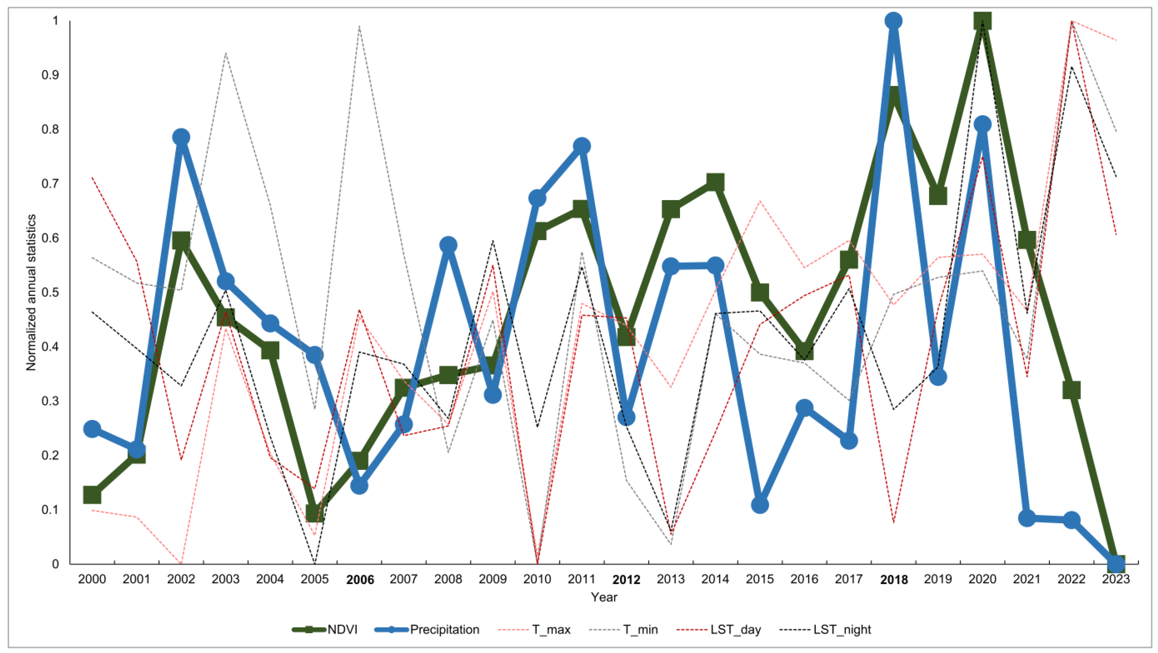
  • The climate factor that most strongly affects NDVI is precipitation. Figure 8 illustrates that the trends of annual NDVI and precipitation over the past 23 years are broadly similar, with both increasing and decreasing almost simultaneously, compared to the other four climate variables.
  • In fact, we believe that the relationship between changes in precipitation and NDVI is not as simple as the one-sided positive correlation suggested by the model. This aligns with the findings of most scholars, indicating a highly complex and strong relationship between the two, which cannot be easily explained by conventional models [25,31,32,33,34,35].
Based on this unresolved complex and important relationship between precipitation and NDVI, we attempted to successfully explain this mechanism by utilizing the precipitation/NDVI characteristic triangle space.
  • The precipitation at the intersection of the two hypotenuses of the characteristic triangle represents a critical value that governs two interactions with NDVI. Above this precipitation, the two variables cooperate and mutually promote each other, while below it, they exhibit a counteractive relationship. This critical value has been increasing each year.
  • The slopes of the two hypotenuses and the area sizes of the two triangles divided by the vertical line both indicate the strength of these interactions. The steeper the slope and the larger the area, the greater the intensity of the interaction, and the more significant its impact on NDVI for that year.
  • As predicted in this study, the dominant relationship in 2012 was the inverse interaction. NDVI was suppressed by precipitation, and the related EQI decreased accordingly. When cross-referencing this with Table 3, we find that the EQI ratio of green land in this year was the lowest among the three years.
  • Additionally, the threshold and total area of the straight side of the characteristic triangle show that the interaction between BMR precipitation and NDVI is becoming increasingly complex.
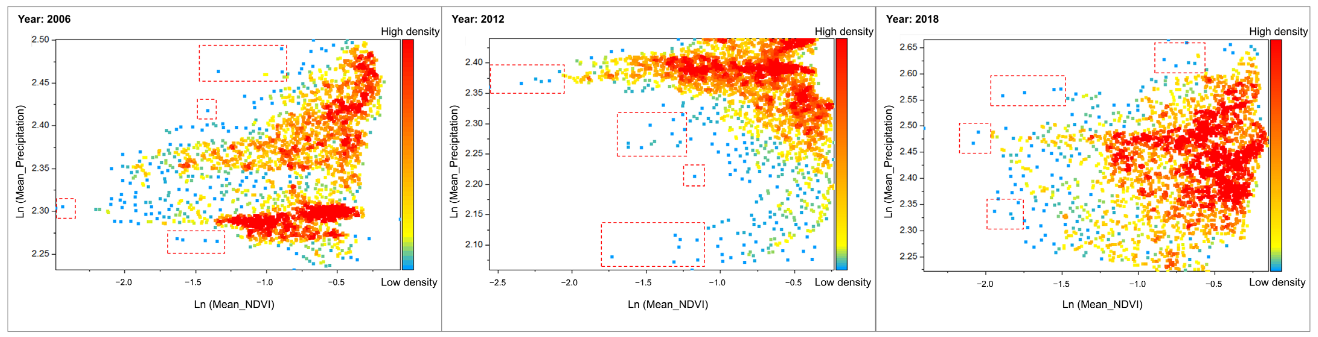
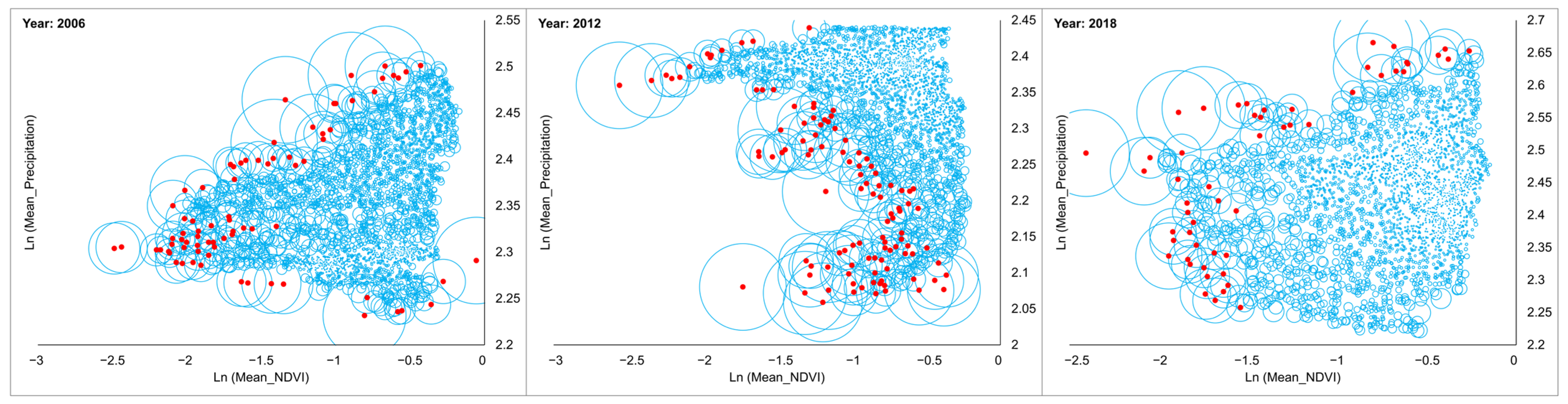
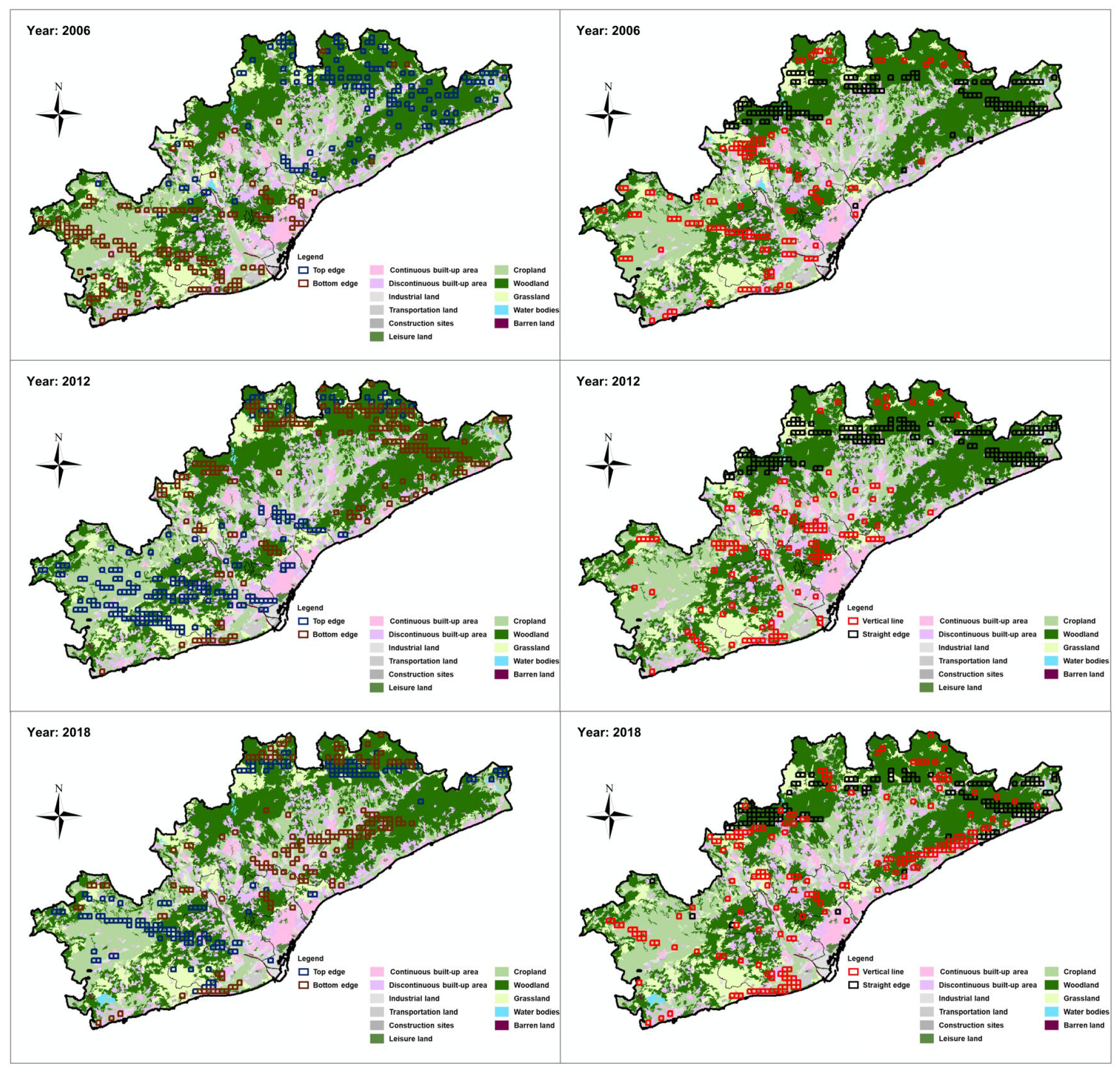
  • Finally, we analyzed the geographical distribution of pixels corresponding to scatter points near the three sides and vertical lines of each characteristic triangle, summarizing their typical land covers and associated EQIs.

5. Discussion

Based on the results of this study, we can confidently conclude that precipitation, which serves as the dividing value between the two effects of precipitation and NDVI, is increasing. This suggests that the lower hypotenuse of the characteristic triangle, representing the possibility of the reverse effect between the two, has become more dominant over time. Against the backdrop of global warming, according to a recent study by Arellano, climate change is leading to a decrease in precipitation [68]. Like most other scholars, they firmly believe that Spain’s climate will be significantly drier and warmer in the coming decades, with more extreme events in this regard [68,69,70,71]. Based on this, we can propose the main objectives for further work: in the future, the relationship between precipitation and NDVI in the BMR may be greatly affected by climate warming, the dividing value between the two effects will continue to increase, the inverse relationship will become more and more dominant, and EQI will also be negatively affected to a certain extent.
In this article, a dynamic ecological environment quality-assessment system is established, which can be applied to changes across different times and regions using NDVI and NDBI. The impact of climate change, human activities, and other natural factors on the evolution of environmental quality is comprehensively considered, and the most critical direct and indirect variables influencing the EQI results are identified. Finally, the characteristic triangular spatial model is developed to analyze precipitation, an important and highly complex climate factor closely related to environmental changes, revealing the underlying mechanism between the two. This study approaches the analysis of two key variables for EQI from a global environmental quality-assessment perspective and provides a deep analysis of how various factors influence environmental quality. However, this study still has certain shortcomings; due to limited technology and data access and the particularity of precipitation and extreme temperature data, their resolution is too large. We adopted a re-interpolation method to obtain data with a more accurate range, which will affect the accuracy of the experimental results. In future research, we will try to use or establish a more accurate database ourselves.
On the other hand, due to the high complexity of the climate system and the intricate feedback loops between its components, remote sensing for climate monitoring presents significant challenges. Generally, climate change research requires data spanning multiple years (for instance, this study covers a period of twelve years) to distinguish the evolution of a specific indicator from its underlying effects or drivers [72]. The challenge lies in the fact that each satellite payload is designed with a finite lifespan. Even when identical sensors are deployed on multiple satellites, the gradual degradation of sensor performance over time can lead to inconsistencies in satellite signals, thus compromising the reliability of remote sensing-based studies on environmental changes [73]. Furthermore, excessively coarse resolution can significantly increase the difficulty of analyzing smaller regions and may affect the accuracy of the results. Therefore, addressing the limitations of current remote sensing technologies by developing more specialized sensors and improving the precision of climate data is essential.

Author Contributions

Conceptualization, X.Z., B.A.R. and J.R.C.; methodology, X.Z.; software, X.Z.; validation, B.A.R. and J.R.C.; formal analysis, X.Z.; resources, X.Z.; data curation, X.Z.; writing—original draft preparation, X.Z., J.R.C. and B.A.R.; writing—review and editing, B.A.R. and J.R.C.; visualization, X.Z.; supervision, B.A.R. and J.R.C.; project administration, J.R.C. and B.A.R.; funding acquisition, J.R.C. and B.A.R. All authors have read the manuscript and made some official changes. All authors have read and agreed to the published version of the manuscript.

Funding

This research received no external funding.

Institutional Review Board Statement

This study did not involve human or animal research; therefore, this statement does not apply.

Informed Consent Statement

This study was used for research not involving humans; therefore, this statement does not apply.

Data Availability Statement

The original contributions presented in this study are included in the article/Appendix A, Appendix B, Appendix C and Appendix D; further inquiries can be directed to the corresponding author.

Acknowledgments

This study is part of the project “Extreme Spatial and Urban Planning Tool for Episodes of Heat Waves and Flash Floods. Building resilience for cities and regions”, supported by the Ministry of Science and Innovation of Spain. Additionally, we must thank Qianhui Zheng (qianhuizheng0712@gmail.com) for her great contribution in providing us with the Spanish annual climate remote sensing database with a resolution of 1° for the period 2000–2023.

Conflicts of Interest

The authors declare no conflicts of interest.

Appendix A

Table A1. BMR land reclassification and land description.
CodeClassification ResultsCLC Land-Use DescriptionCategories
1Continuous built-up areaContinuous urban fabricUrban land
2Discontinuous built-up areaDiscontinuous urban fabric
3Industrial landIndustrial or commercial unitsConstruction land
4Transportation landRoad and rail networks and associated land
Port areas
Airports
5Mine, dump, and construction sitesMineral extraction sites
Dump sites
Construction sites
6Leisure landGreen urban areasGreen area
Sport and leisure facilities
7CroplandNon-irrigated arable land
Permanently irrigated land
Rice fields
Vineyards
Fruit trees and berry plantations
Olive groves
Pastures
Annual crops associated with permanent crops
Complex cultivation patterns
Land principally occupied by agriculture, with significant areas of natural vegetation
Agro-forestry areas
8WoodlandBroad-leaved forest
Coniferous forest
Mixed forest
9GrasslandNatural grasslands
Moors and heathland
Sclerophyllous vegetation
Transitional woodland-shrub
Inland marshes
Peat bogs
Salt marshes
10Barren landBeaches, dunes, sandsBarren land
Bare rocks
Sparsely vegetated areas
Burnt areas
Glaciers and perpetual snow
Salines
Intertidal flats
11Water bodiesWater coursesWater bodies
Water bodies
Coastal lagoons
Estuaries
Sea and ocean
NODATA

Appendix B

Table A2. The EQI assessment results of various types of BMR land use and the land types corresponding to the codes are shown in Table 2.
CodeEQI_2006EQI_2012EQI_2018
100.0092190.003457
20.0005350.0217220.011454
30.0070830.0156540
40.0030320.0025960.001035
50.0028760.0030890.001127
60.0086740.0111140.0076
70.1463740.1572150.125857
80.4261030.420760.417397
90.0948430.0977190.097545
100.001640.0012370.000914
110.00050400.000353
Total0.6916640.7403240.666741

Appendix C

Table A3. Pearson of variables involved in Table 4 _Model 2006 1.
Var123456789101112131415161718192021
11−0.058 **0.176 **0.268 **0.090 **0.448 **0.212 **0.679 **0.114 **−0.463 **−0.549 **−0.124 **−0.300 **−0.421 **0.307 **−0.536 **−0.463 **−0.549 **−0.947 **−0.982 **−0.514 **
2−0.058 **10.705 **−0.283 **0.049 **0.0030.036 *0.312 **0.884 **−0.261 **.331 **−0.501 **0.212 **−0.379 **0.693 **−0.384 **−0.261 **0.331 **0.067 **0.063 **0.068 **
30.176 **0.705 **10.459 **0.053 **0.480 **0.136 **0.405 **0.863 **−0.428 **−0.245 **−0.291 **−0.379 **−0.788 **0.733 **−0.427 **−0.428 **−0.245 **−0.142 **−0.179 **−0.279 **
40.268 **−0.283 **0.459 **10.0120.609 **0.129 **0.144 **0.033−0.267 **−0.692 **0.181 **−0.775 **−0.531 **0.046 *−0.103 **−0.267 **−0.692 **−0.246 **−0.281 **−0.412 **
50.090 **0.049 **0.053 **0.01210.124 **0.068 **0.140 **0.085 **−0.098 **−0.089 **−0.045 *−0.111 **−0.086 **0.021−0.124 **−0.098 **−0.089 **−0.084 **−0.087 **−0.122 **
60.448 **0.0030.480 **0.609 **0.124 **10.206 **0.554 **0.355 **−0.659 **−0.722 **−0.217 **−0.755 **−0.712 **0.307 **−0.523 **−0.659 **−0.722 **−0.420 **−0.452 **−0.734 **
70.212 **0.036 *0.136 **0.129 **0.068 **0.206 **10.409 **0.102 **−0.229 **−0.113 **−0.168 **−0.100 **−0.131 **0.091 **−0.187 **−0.229 **−0.113 **−0.141 **−0.192 **−0.141 **
80.679 **0.312 **0.405 **0.144 **0.140 **0.554 **0.409 **10.447 **−0.804 **−0.328 **−0.638 **−0.263 **−0.513 **0.467 **−0.930 **−0.804 **−0.328 **−0.644 **−0.683 **−0.526 **
90.114 **0.884 **0.863 **0.0330.085 **0.355 **0.102 **0.447 **1−0.422 **−0.022−0.435 **−0.178 **−0.686 **0.770 **−0.496 **−0.422 **−0.022−0.087 **−0.108 **−0.238 **
10−0.463 **−0.261 **−0.428 **−0.267 **−0.098 **−0.659 **−0.229 **−0.804 **−0.422 **10.409 **0.790 **0.364 **0.524 **−0.389 **0.807 **1.000 **0.409 **0.434 **0.471 **0.565 **
11−0.549 **0.331 **−0.245 **−0.692 **−0.089 **−0.722 **−0.113 **−0.328 **−0.0220.409 **1−0.235 **0.689 **0.580 **−0.183 **0.243 **0.409 **1.000 **0.511 **0.558 **0.673 **
12−0.124 **−0.501 **−0.291 **0.181 **−0.045 *−0.217 **−0.168 **−0.638 **−0.435 **0.790 **−0.235 **1−0.075 **0.168 **−0.291 **0.696 **0.790 **−0.235 **0.119 **0.126 **0.150 **
13−0.300 **0.212 **−0.379 **−0.775 **−0.111 **−0.755 **−0.100 **−0.263 **−0.178 **0.364 **0.689 **−0.075 **10.670 **−0.038 *0.218 **0.364 **0.689 **0.289 **0.307 **0.576 **
14−0.421 **−0.379 **−0.788 **−0.531 **−0.086 **−0.712 **−0.131 **−0.513 **−0.686 **0.524 **0.580 **0.168 **0.670 **1−0.767 **0.475 **0.524 **0.580 **0.382 **0.427 **0.666 **
150.307 **0.693 **.733 **0.046 *0.021.307 **0.091 **0.467 **0.770 **−0.389 **−0.183 **−0.291 **−0.038 *−0.767 **1−0.453 **−0.389 **−0.183 **−0.265 **−0.310 **−0.401 **
16−0.536 **−0.384 **−0.427 **−0.103 **−0.124 **−0.523 **−0.187 **−0.930 **−0.496 **0.807 **0.243 **0.696 **0.218 **0.475 **−0.453 **10.807 **0.243 **0.508 **0.539 **0.468 **
17−0.463 **−0.261 **−0.428 **−0.267 **−0.098 **−0.659 **−0.229 **−0.804 **−0.422 **1.000 **0.409 **0.790 **0.364 **0.524 **−0.389 **0.807 **10.409 **0.434 **0.471 **0.565 **
18−0.549 **0.331 **−0.245 **−0.692 **−0.089 **−0.722 **−0.113 **−0.328 **−0.0220.409 **1.000 **−0.235 **0.689 **0.580 **−0.183 **0.243 **0.409 **10.511 **0.558 **0.673 **
19−0.947 **0.067 **−0.142 **−0.246 **−0.084 **−0.420 **−0.141 **−0.644 **−0.087 **0.434 **0.511 **0.119 **0.289 **0.382 **−0.265 **0.508 **0.434 **0.511 **10.945 **0.492 **
20−0.982 **0.063 **−0.179 **−0.281 **−0.087 **−0.452 **−0.192 **−0.683 **−0.108 **0.471 **0.558 **0.126 **0.307 **0.427 **−0.310 **0.539 **0.471 **0.558 **0.945 **10.515 **
21−0.514 **0.068 **−0.279 **−0.412 **−0.122 **−0.734 **−0.141 **−0.526 **−0.238 **0.565 **0.673 **0.150 **0.576 **0.666 **−0.401 **0.468 **0.565 **0.673 **0.492 **0.515 **1
* The correlation is significant at the 0.05 level (two-tailed). ** The correlation is significant at the 0.01 level (two-tailed). 1 The variables corresponding to the code are: 1 Green%, 2 Longitude, 3 Latitude, 4 Distance from coastline, 5 Orientation, 6 Altitude, 7 Slope, 8 NDVI_MEAN, 9 Precipitation, 10 LST_DAY, 11 LST_NIGHT, 12 LST_DAY-LST_NIGHT, 13 T_max, 14 T_min, 15 Tmax-Tmin, 16 NDBI, 17 UHIE_DAY, 18 UHIE_NIGHT, 19 Impermeable area, 20 Artificial area, 21 Night light.
Table A4. Pearson of variables involved in Table 4 _Model 2012 1.
Var123456789101112131415161718192021
11−0.060 **0.178 **0.272 **0.090 **0.456 **0.214 **0.677 **−0.184 **−0.454 **−0.529 **−0.176 **−0.316 **−0.335 **0.197 **−0.553 **−0.454 **−0.529 **−0.953 **−0.981 **−0.510 **
2−0.060 **10.705 **−0.283 **0.049 **0.0030.036 *0.284 **−0.681 **−0.223 **0.047 *−0.303 **−0.430 **−0.353 **0.112 **−0.366 **−0.223 **0.047 *0.020.0320.049 **
30.178 **0.705 **10.459 **0.053 **0.480 **0.136 **0.405 **−0.596 **−0.439 **−0.527 **−0.160 **−0.745 **−0.873 **0.588 **−0.485 **−0.439 **−0.527 **−0.149 **−0.163 **−0.282 **
40.272 **−0.283 **0.459 **10.0120.609 **0.129 **0.185 **0.096 **−0.323 **−0.741 **0.132 **−0.413 **−0.706 **0.660 **−0.211 **−0.323 **−0.741 **−0.194 **−0.218 **−0.393 **
50.090 **0.049 **0.053 **0.01210.124 **0.068 **0.142 **−0.015−0.097 **−0.132 **−0.025−0.112 **−0.051 **−0.033−0.135 **−0.097 **−0.132 **−0.058 *−0.072 **−0.128 **
60.456 **0.0030.480 **0.609 **0.124 **10.206 **0.593 **−0.186 **−0.745 **−0.815 **−0.327 **−0.672 **−0.632 **0.296 **−0.613 **−0.745 **−0.815 **−0.364 **−0.418 **−0.735 **
70.214 **0.036 *0.136 **0.129 **0.068 **0.206 **10.433 **−0.036 *−0.228 **−0.125 **−0.188 **−0.084 **−0.157 **0.154 **−0.249 **−0.228 **−0.125 **−0.142 **−0.181 **−0.146 **
80.677 **0.284 **0.405 **0.185 **0.142 **0.593 **0.433 **1−0.360 **−0.802 **−0.441 **−0.662 **−0.467 **−0.441 **0.207 **−0.922 **−0.802 **−0.441 **−0.665 **−0.709 **−0.566 **
9−0.184 **−0.681 **−0.596 **0.096 **−0.015−0.186 **−0.036 *−0.360 **10.360 **0.181 **0.308 **0.647 **0.443 **−0.0350.368 **0.360 **0.181 **0.156 **0.165 **0.318 **
10−0.454 **−0.223 **−0.439 **−0.323 **−0.097 **−0.745 **−0.228 **−0.802 **0.360 **10.565 **0.812 **0.560 **0.460 **−0.146 **0.811 **10.000 **0.565 **0.364 **0.406 **0.635 **
11−0.529 **0.047 *−0.527 **−0.741 **−0.132 **−0.815 **−0.125 **−0.441 **0.181 **0.565 **1−0.0220.629 **0.729 **−0.484 **0.448 **0.565 **10.000 **0.475 **0.518 **0.664 **
12−0.176 **−0.303 **−0.160 **0.132 **−0.025−0.327 **−0.188 **−0.662 **0.308 **0.812 **−0.02210.234 **0.042 *0.165 **0.668 **0.812 **−0.0220.087 **0.108 **0.301 **
13−0.316 **−0.430 **−0.745 **−0.413 **−0.112 **−0.672 **−0.084 **−0.467 **0.647 **0.560 **0.629 **0.234 **10.756 **−0.163 **0.503 **0.560 **0.629 **0.232 **0.261 **0.592 **
14−0.335 **−0.353 **−0.873 **−0.706 **−0.051 **−0.632 **−0.157 **−0.441 **0.443 **0.460 **0.729 **0.042 *0.756 **1−0.769 **0.475 **0.460 **0.729 **0.285 **0.321 **0.432 **
150.197 **0.112 **0.588 **0.660 **−0.0330.296 **0.154 **0.207 **−0.035−0.146 **−0.484 **0.165 **−0.163 **−0.769 **1−0.223 **−0.146 **−0.484 **−0.199 **−0.226 **−0.075 **
16−0.553 **−0.366 **−0.485 **−0.211 **−0.135 **−0.613 **−0.249 **−0.922 **0.368 **0.811 **0.448 **0.668 **0.503 **0.475 **−0.223 **10.811 **0.448 **0.532 **0.565 **0.540 **
17−0.454 **−0.223 **−0.439 **−0.323 **−0.097 **−0.745 **−0.228 **−0.802 **0.360 **10.000 **0.565 **0.812 **0.560 **0.460 **−0.146 **0.811 **10.565 **0.364 **0.406 **0.635 **
18−0.529 **0.047 *−0.527 **−0.741 **−0.132 **−0.815 **−0.125 **−0.441 **0.181 **0.565 **10.000 **−0.0220.629 **0.729 **−0.484 **0.448 **0.565 **10.475 **0.518 **0.664 **
19−0.953 **0.02−0.149 **−0.194 **−0.058 *−0.364 **−0.142 **−0.665 **0.156 **0.364 **0.475 **0.087 **0.232 **0.285 **−0.199 **0.532 **0.364 **0.475 **10.942 **0.355 **
20−0.981 **0.032−0.163 **−0.218 **−0.072 **−0.418 **−0.181 **−0.709 **0.165 **0.406 **0.518 **0.108 **0.261 **0.321 **−0.226 **0.565 **0.406 **0.518 **0.942 **10.389 **
21−0.510 **0.049 **−0.282 **−0.393 **−0.128 **−0.735 **−0.146 **−0.566 **0.318 **0.635 **0.664 **0.301 **0.592 **0.432 **−0.075 **0.540 **0.635 **0.664 **0.355 **0.389 **1
* The correlation is significant at the 0.05 level (two-tailed). ** The correlation is significant at the 0.01 level (two-tailed). 1 The variables corresponding to the code are: 1 Green%, 2 Longitude, 3 Latitude, 4 Distance from coastline, 5 Orientation, 6 Altitude, 7 Slope, 8 NDVI_MEAN, 9 Precipitation, 10 LST_DAY, 11 LST_NIGHT, 12 LST_DAY-LST_NIGHT, 13 T_max, 14 T_min, 15 Tmax-Tmin, 16 NDBI, 17 UHIE_DAY, 18 UHIE_NIGHT, 19 Impermeable area, 20 Artificial area, 21 Night light.
Table A5. Pearson of variables involved in Table 4 _Model 2018 1.
Var123456789101112131415161718192021
11−0.049 **0.192 **0.280 **0.088 **0.461 **0.213 **0.688 **0.125 **−0.547 **−0.576 **−0.303 **−0.305 **−0.376 **0.242 **−0.589 **−0.547 **−0.576 **−0.944 **−0.978 **−0.560 **
2−0.049 **10.705 **−0.283 **0.049 **0.0030.036 *0.334 **−0.039 *−0.136 **−0.008−0.172 **−0.409 **−0.312 **−0.018−0.370 **−0.136 **−0.0080.070 **0.060 **0.002
30.192 **0.705 **10.459 **0.053 **0.480 **0.136 **0.442 **−0.207 **−0.464 **−0.509 **−0.241 **−0.784 **−0.858 **0.431 **−0.473 **−0.464 **−0.509 **−0.145 **−0.186 **−0.349 **
40.280 **−0.283 **0.459 **10.0120.609 **0.129 **0.174 **−0.127 **−0.449 **−0.616 **−0.146 **−0.515 **−0.732 **0.585 **−0.184 **−0.449 **−0.616 **−0.251 **−0.283 **−0.420 **
50.088 **0.049 **0.053 **0.01210.124 **0.068 **0.145 **0.074 **−0.065 **−0.138 **0.014−0.123 **−0.060 **−0.065 **−0.145 **−0.065 **−0.138 **−0.088 **−0.088 **−0.081 **
60.461 **0.0030.480 **0.609 **0.124 **10.206 **0.554 **0.152 **−0.806 **−0.741 **−0.522 **−0.715 **−0.670 **0.193 **−0.587 **−0.806 **−0.741 **−0.430 **−0.465 **−0.759 **
70.213 **0.036 *0.136 **0.129 **0.068 **0.206 **10.425 **0.042 *−0.226 **−0.112 **−0.215 **−0.104 **−0.165 **0.150 **−0.391 **−0.226 **−0.112 **−0.194 **−0.202 **−0.179 **
80.688 **0.334 **0.442 **0.174 **0.145 **0.554 **0.425 **10.229 **−0.768 **−0.456 **−0.675 **−0.479 **−0.466 **0.155 **−0.948 **−0.768 **−0.456 **−0.659 **−0.692 **−0.595 **
90.125 **−0.039 *−0.207 **−0.127 **0.074 **0.152 **0.042 *0.229 **1−0.264 **−0.062 **−0.300 **−0.054 **0.111 **−0.273 **−0.275 **−0.264 **−0.062 **−0.145 **−0.125 **−0.204 **
10−0.547 **−0.136 **−0.464 **−0.449 **−0.065 **−0.806 **−0.226 **−0.768 **−0.264 **10.649 **0.840 **0.631 **0.590 **−0.168 **0.776 **10.000 **0.649 **0.509 **0.553 **0.770 **
11−0.576 **−0.008−0.509 **−0.616 **−0.138 **−0.741 **−0.112 **−0.456 **−0.062 **0.649 **10.132 **0.650 **0.750 **−0.427 **0.427 **0.649 **10.000 **0.536 **0.585 **0.722 **
12−0.303 **−0.172 **−0.241 **−0.146 **0.014−0.522 **−0.215 **−0.675 **−0.300 **0.840 **0.132 **10.359 **0.234 **0.086 **0.705 **0.840 **0.132 **0.281 **0.304 **0.488 **
13−0.305 **−0.409 **−0.784 **−0.515 **−0.123 **−0.715 **−0.104 **−0.479 **−0.054 **0.631 **0.650 **0.359 **10.829 **−0.077 **0.504 **0.631 **0.650 **0.279 **0.308 **0.609 **
14−0.376 **−0.312 **−0.858 **−0.732 **−0.060 **−0.670 **−0.165 **−0.466 **0.111 **0.590 **0.750 **0.234 **0.829 **1−0.621 **0.464 **0.590 **0.750 **0.330 **0.385 **0.556 **
150.242 **−0.0180.431 **0.585 **−0.065 **0.193 **0.150 **0.155 **−0.273 **−0.168 **−0.427 **0.086 **−0.077 **−0.621 **1−0.118 **−0.168 **−0.427 **−0.197 **−0.255 **−0.138 **
16−0.589 **−0.370 **−0.473 **−0.184 **−0.145 **−0.587 **−0.391 **−0.948 **−0.275 **0.776 **0.427 **0.705 **0.504 **0.464 **−0.118 **10.776 **0.427 **0.564 **0.592 **0.575 **
17−0.547 **−0.136 **−0.464 **−0.449 **−0.065 **−0.806 **−0.226 **−0.768 **−0.264 **10.000 **0.649 **0.840 **0.631 **0.590 **−0.168 **0.776 **10.649 **0.509 **0.553 **0.770 **
18−0.576 **−0.008−0.509 **−0.616 **−0.138 **−0.741 **−0.112 **−0.456 **−0.062 **0.649 **10.000 **0.132 **0.650 **0.750 **−0.427 **0.427 **0.649 **10.536 **0.585 **0.722 **
19−0.944 **0.070 **−0.145 **−0.251 **−0.088 **−0.430 **−0.194 **−0.659 **−0.145 **0.509 **0.536 **0.281 **0.279 **0.330 **−0.197 **0.564 **0.509 **0.536 **10.946 **0.536 **
20−0.978 **0.060 **−0.186 **−0.283 **−0.088 **−0.465 **−0.202 **−0.692 **−0.125 **0.553 **0.585 **0.304 **0.308 **0.385 **−0.255 **0.592 **0.553 **0.585 **0.946 **10.571 **
21−0.560 **0.002−0.349 **−0.420 **−0.081 **−0.759 **−0.179 **−0.595 **−0.204 **0.770 **0.722 **0.488 **0.609 **0.556 **−0.138 **0.575 **0.770 **0.722 **0.536 **0.571 **1
* The correlation is significant at the 0.05 level (two-tailed). ** The correlation is significant at the 0.01 level (two-tailed). 1 The variables corresponding to the code are: 1 Green%, 2 Longitude, 3 Latitude, 4 Distance from coastline, 5 Orientation, 6 Altitude, 7 Slope, 8 NDVI_MEAN, 9 Precipitation, 10 LST_DAY, 11 LST_NIGHT, 12 LST_DAY-LST_NIGHT, 13 T_max, 14 T_min, 15 Tmax-Tmin, 16 NDBI, 17 UHIE_DAY, 18 UHIE_NIGHT, 19 Impermeable area, 20 Artificial area, 21 Night light.

Appendix D

Table A6. Pearson of variables involved in Table 5 _Model.
NDVIPrecipitationT_maxT_minLST_dayLST_night
NDVI10.684 **0.053−0.283−0.2360.131
Precipitation0.684 **1−0.388−0.256−0.484 *−0.168
T_max0.053−0.38810.433 *0.593 **0.670 **
T_min−0.283−0.2560.433 *10.563 **0.555 **
LST_day−0.236−0.484 *0.593 **0.563 **10.817 **
LST_night0.131−0.1680.670 **0.555 **0.817 **1
** The correlation is significant at the 0.01 level (two-tailed). * Correlation is significant at the 0.05 level (two-tailed).

References

  1. Liu, T. Evaluation of Guilin’s urban ecological environment based on remote sensing data. Master’s Thesis, Guilin University of Technology, Guilin, China, 2023. [Google Scholar]
  2. Ramez, A.B.; Hooi, H.L.; Jeremy, C. The evolution of the natural resource curse thesis: A critical literature survey. Resour. Policy 2017, 51, 123–134. [Google Scholar]
  3. Qian, L.; Wu, Z.; Guo, G. Research on the relationship between built environment and urban biodiversity in high-density urban areas: Taking Century Avenue in Pudong New Area, Shanghai as an example. Urban Dev. Res. Res. 2018, 25, 97–106. [Google Scholar]
  4. Xiong, K.; Li, J.; Long, M. Characteristics and key issues of soil and water loss in typical karst rocky desertification control areas. Chin. J. Geogr. 2012, 67, 878–888. [Google Scholar]
  5. Roca, J.; Arellano, B. Effects of urban greenery on health. A study from remote sensing. Int. Arch.Photogramm. Remote Sens. Spat. Inf. Sci. 2022, XLIII-B3-2022, 17–24. [Google Scholar]
  6. Xu, Z.; Blanca, A. Urban sprawl and warming—Research on the evolution of the urban sprawl of chinese municipalities and its relationship with climate warming in the past three decades. Int. Arch.Photogramm. Remote Sens. Spat. Inf. Sci. 2022, XLIII-B4-2022, 209–215. [Google Scholar]
  7. Wang, F.; Liang, R.; Yang, X.; Chen, M. Research on ecological water demand in northwest China—Theoretical analysis of ecological water demand in Arid and Semi-arid Regions. J. Nat. Resour. 2002, 2010, 1–8. [Google Scholar]
  8. Wang, Z. Chahannaoer basin based on improved remote sensing ecological index. Master’s Thesis, Anhui University of Science and Technology, Huainan, China, 2021. [Google Scholar]
  9. Lavorel, S.; Flannigan, M.D.; Lambin, E.F. Vulnerability of land systems to fire: Interactions among humans, climate, the atmosphere, and ecosystems. Mitig. Adapt. Strateg. Glob. Change 2007, 12, 33–53. [Google Scholar] [CrossRef]
  10. Moran, M.S.; Peters, C.D.; Watts, J.M. Estimating soil moisture at the watershed scale with satellite-based radar and land surface models. Can. J. Remote Sens. 2004, 30, 805–826. [Google Scholar] [CrossRef]
  11. Gupta, K.; Kumar, P.; Pathan, S.K. Urban Neighborhood Green Index—A measures of green spaces inutban areas. Landsc. Urban Plan. 2012, 105, 325–335. [Google Scholar] [CrossRef]
  12. Wickham, J.D.; Jones, K.B. Environmental auditing, An Integrated Environmental Assessment of the US Mid-Atlantic Region. Environ. Manag. 1999, 24, 553–560. [Google Scholar] [CrossRef]
  13. Ivits, E.; Cherlet, M.; Mehl, W.; Sommer, S. Estimating the ecologic status and change of riparian zones in Andalusia assessed by multi-temporal AVHHR data. Ecol Indie 2009, 9, 422–431. [Google Scholar] [CrossRef]
  14. Manill, J.; Pino, J.; Mallarach, J.M. A land suitability index for strategic environmental assessment in metropolitan areas. Landsc. Urban Plan. 2017, 201, 200. [Google Scholar]
  15. Xu, H. Remote sensing evaluation index of regional ecological environment change. China Environ. Sci. 2013, 33, 889–897. [Google Scholar]
  16. Hou, Y.; Chen, Y.; Ding, J.; Li, Z.; Li, Y.; Sun, F. Ecological Impacts of Land Use Change in the Arid Tarim River Basin of China. Remote Sens. 2022, 14, 1894. [Google Scholar] [CrossRef]
  17. Wessels, K.; Prince, S.; Frost, P. Assessing the effects of human-induced land degradation in the former homelands of northern south africa with a 1 km AVHRR NDVI time-series. Remote Sens. Environ. 2004, 91, 47–67. [Google Scholar] [CrossRef]
  18. Pettorelli, N.; Laurance, W.; O’Brien, T. Satellite remote sensing for applied ecologists: Opportunities and challenges. J. Appl. Ecol. 2014, 51, 839–848. [Google Scholar] [CrossRef]
  19. Goward, S.; Prince, S. Transient effects of climate on vegetation dynamics: Satellite observations. J. Biogeogr. 1995, 22, 549–563. [Google Scholar] [CrossRef]
  20. De Jong, S.; Brouwer, L.; Riezebos, H. Effects of grazing on vegetation and erosion in the chaco boreal, paraguay. Geoderma 1999, 88, 65–79. [Google Scholar]
  21. Jie, R. Study on the evolution and driving force of surface ecological environment in western lli basin based on NDVI. Master’s Thesis, College of Disaster Prevention Technology, Langfang, China, 2020. [Google Scholar]
  22. Zhang, Y.; She, J.; Long, X.; Zhang, M. Spatial-temporal evolution and driving factors of eco-environmental quality based on RSEI in Chang-Zhu-Tan metropolitan circle, central China. Ecol. Indic. 2022, 144, 109436. [Google Scholar] [CrossRef]
  23. Zhang, L.; Fang, C.; Zhao, R.; Zhu, C.; Guan, J. Spatial-temporal evolution and driving force analysis of eco-quality in urban agglomerations in China. Sci. Total Environ. 2023, 866, 161465. [Google Scholar] [CrossRef]
  24. Huang, M.; Gong, D.; Zhang, L.; Lin, H.; Chen, Y.; Zhu, D.; Xiao, C.; Altan, O. Spatial-temporal dynamics and forecasting of ecological security pattern under the consideration of protecting habitat: A case study of the Poyang Lake ecoregion. Int. J. Digit. Earth 2024, 17, 2376277. [Google Scholar] [CrossRef]
  25. Xu, Z.; Arellano, B.; Roca, J. Study on factors influencing forest distribution in Barcelona metropolitan region. Sustainability 2024, 16, 5449. [Google Scholar] [CrossRef]
  26. Zhou, L.; Tucker, C.; Kaufmann, R.K. Variations in northern vegetation activity inferred from satellite data of vegetation index during 1981 to 1999. J. Geophys. Res. 2001, 106, 20069–20083. [Google Scholar] [CrossRef]
  27. Yang, Y.; Shang, S.; Mao, Q. Impact of soil moisture on vegetation growing condition and climate change over the Tibetan plateau. J. Geophys. Res. Atmos. 2012, 117, 15205–15215. [Google Scholar]
  28. Wu, C.; Niu, Z.; Tang, Q. Impact of topography on vegetation dynamics in a mountain-oasis-desert system in Xinjiang, China. Remote Sens. 2018, 10, 946. [Google Scholar]
  29. Xu, C.; Liu, M.; Zhang, Z. Responses of vegetation activity to multi-factor influences in different sub-regions of northeast China. Remote Sens. 2014, 6, 5866–5887. [Google Scholar]
  30. Ji, L.; Peters, A. Assessing vegetation response to drought in the northern great plains using vegetation and drought indices. Remote Sens. Environ. 2003, 87, 85–98. [Google Scholar] [CrossRef]
  31. Pettorelli, N.; Vik, J.; Mysterud, A. Using the satellite-derived NDVI to assess ecological responses to environmental change. Trends Ecol. Evol. 2005, 20, 503–510. [Google Scholar] [CrossRef]
  32. Liu, Z.; Li, J. Response of temporal and spatial changes of vegetation in Heilongjiang Province to climate factors from 2000 to 2020. For. Eng. 2024, 40, 85–97. [Google Scholar]
  33. Mu, S.; Li, J.; Chen, Y. Spatial and temporal variation characteristics of vegetation coverage in Inner Mongolia from 2001 to 2010. Acta Geogr. Sin. 2012, 67, 1255–1268. [Google Scholar]
  34. Liu, Y.; Van Dijk, A.; De Jeu, R. Recent reversal in loss of global terrestrial biomass. Nat. Clim. Change 2015, 5, 470–474. [Google Scholar] [CrossRef]
  35. Xu, Y.; Li, J.; Guo, Q.; Li, H.; Wu, H. Spatial-temporal evolution characteristics of NDVI and analysis of its climate driving factors in Nanchang. For. Eng. 2024, 40, 8023. [Google Scholar]
  36. Cebollada, A.; Carme, M. La movilidad en la Región Metropolitana de Barcelona: Entre los nuevos retos y las viejas prácticas. Finisterra 2010, 45, 90. [Google Scholar] [CrossRef]
  37. Available online: https://landscan.ornl.gov/ (accessed on 10 July 2024).
  38. Available online: https://territori.gencat.cat/ca/01_departament/05_plans/01_planificacio_territorial/plans_territorials_nou/territorials_parcials/ptp_metropolita_de_barcelona/ (accessed on 20 September 2024).
  39. Zhang, X.; Roca, J.; Arellano, B. Evolution of ecological patterns of land use changes in European metropolitan areas. In Proceedings of the SPIE, Berlin, Germany, 26 October 2022. [Google Scholar]
  40. Haobo, Y.; Xinyi, Z. Urban heat island analysis based on high resolution measurement data: A case study in Beijing. Sustainable Cities Soc. 2024, 106, 105389. [Google Scholar]
  41. Boer, E.P.; Kirsten, M.; Dewi, H. Kriging and thin plate splines for mapping climate variables. Int. J. Appl. Earth Obs. Geoinf. 2001, 3, 146–154. [Google Scholar] [CrossRef]
  42. Xu, Z.; Roca, J.; Arellano, B. Research on the expansion of Beijing-Tianjin-Hebei China’s Capital metropolitan agglomeration based on night lighting technology. In Proceedings of the SPIE, Amsterdam, The Netherlands, 19 October 2023. [Google Scholar]
  43. Chris, B.; Aysin, D.; Jason, B. Factors shaping urban green space provision: A systematic review of the literature. Landsc. Urban Plan. 2018, 178, 82–101. [Google Scholar]
  44. Rahmati, L.; Hanaei, T. Comparative analysis of key factors influencing urban green space in Mashhad, Iran (1988–2018). Environ. Syst. Res. 2024, 13, 13. [Google Scholar] [CrossRef]
  45. Ghebrezgabher, M.G.; Yang, T.; Yang, X.; Sereke, T.E. Assessment of NDVI variations in responses to climate change in the Horn of Africa. Egypt. J. Remote Sens. Space Sci. 2020, 23, 249–261. [Google Scholar] [CrossRef]
  46. Song, Z. The triangular feature space between nighttime light intensity and vegetation index and its applications. Master’s Thesis, East China Normal University, Shanghai, China, 2023. [Google Scholar]
  47. Sandholt, I.; Rasmussen, K.; Andersen, J. A simple interpretation of the surface temperature/vegetation index space for assessment of surface moisture status. Remote Sens. Environ. 2002, 79, 213–224. [Google Scholar] [CrossRef]
  48. Pengxin, W.; Jianya, G.; Xiaowen, L. Conditional vegetation temperature index and its application in drought monitoring. J. Wuhan Univ. 2001, 26, 412–418. [Google Scholar]
  49. Hasan, M.M.; Croke, B.F.W.; Liu, S.; Shimizu, K.; Karim, F. Using mixed probability distribution functions for modelling non-zero sub-daily rainfall in Australia. Geosciences 2020, 10, 43. [Google Scholar] [CrossRef]
  50. Rosenblatt, M. Remarks on some nonparametric estimates of a density function. Ann. Math. Stat. 1956, 27, 832–837. [Google Scholar] [CrossRef]
  51. Emanuel, P. On estimation of a probability density function and mode. Ann. Math. Stat. 1962, 33, 1065–1076. [Google Scholar]
  52. Epanechnikov, A. Non-Parametric Estimation of a multivariate probability density. Theory Probab. Its Appl. 1969, 14, 153–158. [Google Scholar] [CrossRef]
  53. Xiong, K.; Ding, Q.; Zhu, Z. Chiller fault detection based on isolation forest and KDE-LOF. Comput. Appl. Softw. 2023, 40, 84–89. [Google Scholar]
  54. Breunig, M.; Kriegel, H. LOF: Identifying density-based local outliers. ACM Sigmod Rec. 2000, 29, 93–104. [Google Scholar] [CrossRef]
  55. Wu, Z. Study on Vegetation Cover Change and Its Response to Climate in Qilian Mountains from 2000 to 2012. Master’s Thesis, Northwest Normal University, Lanzhou, China, 2014. [Google Scholar]
  56. Yao, X.; Yu, K.; Liu, J. Spatial and temporal evolution of ecological vulnerability in areas with severe soil erosion in southern China. Chin. J. Appl. Ecol. 2016, 27, 735–745. [Google Scholar]
  57. Zhang, H.; Wang, X.; Peng, D. Evaluation of Urban Vegetation Phenology Using 250 m MODIS Vegetation Indices. Photogramm. Eng. Remote Sens. 2022, 88, 461–467. [Google Scholar] [CrossRef]
  58. Huang, J. Research on forest aboveground biomass regeneration method based on BEPS model and remote sensing. Master’s Thesis, Nanjing University, Nanjing, China, 2014. [Google Scholar]
  59. Cheng, M.; Jiang, H.; Chen, J.; Guo, Z.; Jiang, Z. Study on vegetation cover change in Hotan area of Xinjiang based on Landsat data. J. Anhui Agric. Sci. 2009, 37, 1239–1244. [Google Scholar]
  60. Arellano, B.; Roca, J. Modelling nighttime air temperature from remote sensing imagery and GIS data. In Proceedings of the SPIE, Space, Satellites, and Sustainability II, Glasgow, UK, 28 September–1 October 2021. [Google Scholar]
  61. Zhang, S.; Yang, P.; Xia, J.; Qi, K.; Wang, W.; Cai, W.; Chen, N. Research and Analysis of Ecological Environment Quality in the Middle Reaches of the Yangtze River Basin between 2000 and 2019. Remote Sens. 2021, 13, 4475. [Google Scholar] [CrossRef]
  62. Shi, M.; Lin, F.; Jing, X.; Li, B.; Shi, Y.; Hu, Y. Ecological Environment Quality Assessment of Arid Areas Based on Improved Remote Sensing Ecological Index—A Case Study of the Loess Plateau. Sustainability 2023, 15, 13881. [Google Scholar] [CrossRef]
  63. Zaitunah, A.; Samsuri; Silitonga, A.; Syaufina, L. Urban Greening Effect on Land Surface Temperature. Sensors 2022, 22, 4168. [Google Scholar] [CrossRef] [PubMed]
  64. Peng, L.; Wu, H.; Li, Z. Spatial–Temporal Evolutions of Ecological Environment Quality and Ecological Resilience Pattern in the Middle and Lower Reaches of the Yangtze River Economic Belt. Remote Sens. 2023, 15, 430. [Google Scholar] [CrossRef]
  65. Guha, S.; Govil, H.; Dey, A.; Gill, N. Analytical study of land surface temperature with NDVI and NDBI using Landsat 8 OLI and TIRS data in Florence and Naples city, Italy. Eur. J. Remote Sens. 2018, 51, 667–678. [Google Scholar] [CrossRef]
  66. Xia, W.; Xiaojie, Y.; Changzheng, J.; Wei, D. Dynamic monitoring and analysis of factors influencing ecological environment quality in northern Anhui, China, based on the Google Earth Engine. Sci. Rep. 2022, 12, 20307. [Google Scholar]
  67. Available online: https://land.copernicus.eu/en/products/corine-land-cover/clc2018 (accessed on 16 July 2024).
  68. Arellano, B.; Roca, J.; Qianhui, Z. Spain: Towards a drier and warmer climate? Analysis of climate change effects on precipitation and temperature trends in Spain. In Proceedings of the European Meteorological Society Annual Meeting, Barcelona, Spain, 2 September 2024. [Google Scholar]
  69. Haisheng, H.; Hewitt, R.J. Future climate risks to world cultural heritage sites in Spain: A systematic analysis based on shared socioeconomic pathways. Int. J. Disaster Risk Reduct. 2024, 113, 2212–4209. [Google Scholar]
  70. Lorenzo, M.; Alvarez, I. Future changes of hot extremes in Spain: Towards warmer conditions. Nat Hazards 2022, 113, 383–402. [Google Scholar] [CrossRef]
  71. David, C.; Susana, C.; Rocha, A. Future surface temperature changes for the Iberian Peninsula according to EURO-CORDEX climate projections. Clim. Dyn. 2021, 56, 1–16. [Google Scholar]
  72. Henson, S.; Beaulieu, C.; Lampitt, R. Observing climate change trends in ocean biogeochemistry: When and where. Glob. Change Biol. 2016, 22, 1561–1571. [Google Scholar] [CrossRef]
  73. Chander, G.; Hewison, T.; Fox, N.; Wu, X.; Xiong, X.; Blackwell, W. Overview of intercalibration of satellite instruments. IEEE Trans. Geosci. Remote Sens. 2013, 51, 1056–1080. [Google Scholar] [CrossRef]
Figure 1. Barcelona Metropolitan Region (BMR, with municipalities). (a) BMR satellite aerial photography; (b) BMR mountain elevation map.
Remotesensing 16 04735 g001
Figure 2. Research idea map.
Remotesensing 16 04735 g002
Figure 3. Ecological environment quality-assessment parameters of various types of land use in the BMR during 2006–2018. (a) Ecological environment quality-assessment parameters of various types of land use in the BMR; (b) main categories and overall ecological environment quality-assessment parameters of the BMR. Note: The codes of various types of land use in Figure (a) correspond to Table 2.
Remotesensing 16 04735 g003
Figure 4. Evolution of BMR green area distribution from 2006 to 2018.
Remotesensing 16 04735 g004
Figure 5. Evolution of the BMR green area and number of plaques from 2006 to 2018. (a) Evolution of the BMR green area and proportion of the BMR area; (b) number of BMR green plaques and proportion of plaques to green area.
Remotesensing 16 04735 g005
Figure 6. EQI of various types of land use in BMR green areas from 2006 to 2018.
Remotesensing 16 04735 g006
Figure 7. Spatial distribution map of EQI assessment results in the BMR from 2006 to 2018 (ac). Spatial distribution map of EQI in the BMR from 2006 to 2018; (d) Spatial variation in EQI in the BMR.
Remotesensing 16 04735 g007
Figure 8. Trends in the annual normalized statistical results of the average NDVI and climate factors of the BMR from 2000 to 2023.
Remotesensing 16 04735 g008
Figure 9. The expected triangular spatial structure of the scatter plots of Ln (Mean_NDVI) and Ln (Mean_Precipitation) of the BMR in 2006, 2012, and 2018. Note: The red dashed line delimits the possible triangular distribution structure of the scattered points.
Remotesensing 16 04735 g009
Figure 10. Illustration of the characteristic triangular spatial structure of the precipitation/NDVI scatter plot.
Remotesensing 16 04735 g010
Figure 11. Density distribution of precipitation/NDVI scatter points in the BMR in 2006, 2012, and 2018. Note: The red dashed box encloses the scattered points of low-density distribution.
Remotesensing 16 04735 g011
Figure 12. Results of local anomaly detection of precipitation/NDVI in the BMR in 2006, 2012, and 2018.
Remotesensing 16 04735 g012
Figure 13. Fitting equation of NDVI maximum precipitation between sub-regions in 2006 (example).
Remotesensing 16 04735 g013
Figure 14. Schematic diagram of the precipitation/NDVI characteristic triangle space of the BMR in 2006, 2012, and 2018. Note:The fitted triangular spatial structure is represented by the red solid line.
Remotesensing 16 04735 g014
Figure 15. Pixel distribution of each edge of the land cover and precipitation/NDVI characteristic triangle of the BMR in 2006, 2012, and 2018.
Remotesensing 16 04735 g015
Table 1. List of factors potentially influencing the key land-use distribution.
TypeFactors
Natural factorsLongitude
Latitude
Distance from coastline
Orientation
Altitude
NDVI
Precipitation
LST
LST_day- LST_night
T_max
T_min
T_max-T_min
Human activityNDBI
Urban heat island effect
Impermeable area
Artificial area
Nighttime light data
Table 2. BMR land is reclassified and assigned to major categories *.
CodeReclassificationCategories
1Continuous built-up areaUrban land
2Discontinuous built-up area
3Industrial landConstruction land
4Transportation land
5Construction sites
6Leisure landGreen area
7Cropland
8Woodland
9Grassland
10Water bodiesWater bodies
11Barren landBarren land
* A detailed description of the land uses included in each reclassification can be found in Appendix A.
Table 3. BMR Ecological Environment Quality Index (EQI) evaluation results and the proportion of land-use results of individual categories in the total results.
Categories200620122018
EQI% of TotalEQI% of TotalEQI% of Total
Urban land0.0010.08%0.0314.18%0.0152.24%
Construction land0.0131.88%0.0212.88%0.0020.32%
Green area0.67697.73%0.68792.77%0.64897.25%
Water bodies0.0020.24%0.0010.17%0.0010.14%
Barren land0.0010.07%0.00000.00030.05%
Overall0.692100.00%0.740100.00%0.667100.00%
Table 4. Green area proportion OLS models.
Independent Variable bModel_2006 aModel_2012 aModel_2018 a
BBetatSig.BBetatSig.BBetatSig.
Constant−1719.33 −6.000.00−1534.85 −4.790.00−2681.47 −5.750.00
Longitude0.00−0.17−7.020.000.00−0.12−4.260.000.00−0.16−3.860.00
Latitude0.000.195.410.000.000.174.920.000.000.315.490.00
Distance from coastline0.00−0.13−5.650.000.00−0.08−4.310.000.00−0.06−2.130.03
Orientation0.000.00−0.130.890.000.00−0.760.450.000.00−0.740.46
Altitude0.00−0.02−2.130.030.000.000.330.740.000.000.180.86
Slope2.780.048.590.000.290.000.540.591.610.024.220.00
NDVI_
MEAN
6.770.000.250.805.980.031.890.065.450.031.730.08
Precipitation1.210.031.420.160.970.022.130.030.930.033.890.00
LST_DAY-
LST_NIGHT
0.220.022.010.04−0.12−0.01−0.820.410.180.011.300.20
T_max0.500.011.380.170.830.021.530.134.030.148.050.00
T_max-T_min−1.03−0.03−3.180.00−0.76−0.03−1.950.05−3.55−0.09−7.830.00
NDBI−1.90−0.01−0.870.38−1.920.021.610.11−1.000.021.160.25
UHIE_
NIGHT
−0.020.00−0.130.900.650.032.280.02−0.27−0.01−1.080.28
Impermeable area−15.53−0.15−12.840.00−25.96−0.25−17.790.00−15.74−0.15−10.930.00
Artificial area−80.61−0.83−64.970.00−72.64−0.75−49.370.00−81.32−0.83−56.550.00
Night Light−0.03−0.02−2.550.01−0.02−0.01−1.330.190.010.000.500.62
a The dependent variable of the three models is the proportion of green area in that year. b LST_DAY, LST_NIGHT, T_min, and UHIE_DAY became excluded independent variables during the regression analysis.
Table 5. Multiple OLS models between mean NDVI and various climate factors a.
Independent VariableR2BBetatSig.
Precipitation0.470.000.684.400.00
T_max0.000.000.050.250.81
T_min0.08−0.01−0.28−1.390.18
LST_day0.060.00−0.24−1.140.27
LST_night0.020.000.130.620.54
a The dependent variable for all models is the annual mean NDVI.
Table 6. The spatial three-side fitting results of the precipitation/NDVI characteristic triangle of the BMR in 2006, 2012, and 2018.
YearTop EdgeR2Bottom EdgeR2Straight Edge
2006y = 0.0991x + 2.50460.7510288y = −0.0258x + 2.25630.1790952x = −0.1705
2012y = 0.0261x + 2.44280.2359837y = −0.0841x + 2.21530.5709729x = −0.2341
2018y = 0.113x + 2.65670.375945y = −0.1641x + 2.13390.6198449x = −0.3823
Table 7. Summary of parameters of the spatial structure of precipitation/NDVI characteristic triangles in the BMR in 2006, 2012, and 2018 a.
Year200620122018
Max Precipitation2.49(12.01)2.44(11.43)2.64(14.00)
Min Precipitation2.26(9.59)2.24(9.35)2.16(8.67)
Intersection point_Precipitation2.31(10.05)2.39(10.90)2.44(11.51)
Intersection point_Min NDVI−1.99(0.14)−2.06(0.13)−1.89(0.15)
Max NDVI−0.19(0.83)−0.24(0.79)−0.16(0.85)
Straight edge length0.220.200.48
Wet edge slope0.100.030.11
Dry edge slope−0.03−0.08−0.16
Top triangle area0.160.040.17
Bottom triangle area0.040.140.24
Total area0.200.180.41
a The original value of the parameter is shown in italics and in parentheses.
Disclaimer/Publisher’s Note: The statements, opinions and data contained in all publications are solely those of the individual author(s) and contributor(s) and not of MDPI and/or the editor(s). MDPI and/or the editor(s) disclaim responsibility for any injury to people or property resulting from any ideas, methods, instructions or products referred to in the content.

