Blind Infrared Remote-Sensing Image Deblurring Algorithm via Edge Composite-Gradient Feature Prior and Detail Maintenance

Abstract

The problem of blind image deblurring remains a challenging inverse problem, due to the ill-posed nature of estimating unknown blur kernels and latent images within the Maximum A Posteriori (MAP) framework. To address this challenge, traditional methods often rely on sparse regularization priors to mitigate the uncertainty inherent in the problem. In this paper, we propose a novel blind deblurring model based on the MAP framework that leverages Composite-Gradient Feature (CGF) variations in edge regions after image blurring. This prior term is specifically designed to exploit the high sparsity of sharp edge regions in clear images, thereby effectively alleviating the ill-posedness of the problem. Unlike existing methods that focus on local gradient information, our approach focuses on the aggregation of edge regions, enabling better detection of both sharp and smoothed edges in blurred images. In the blur kernel estimation process, we enhance the accuracy of the kernel by assigning effective edge information from the blurred image to the smoothed intermediate latent image, preserving critical structural details lost during the blurring process. To further improve the edge-preserving restoration, we introduce an adaptive regularizer that outperforms traditional total variation regularization by better maintaining edge integrity in both clear and blurred images. The proposed variational model is efficiently implemented using alternating iterative techniques. Extensive numerical experiments and comparisons with state-of-the-art methods demonstrate the superior performance of our approach, highlighting its effectiveness and real-world applicability in diverse image-restoration tasks.

1. Introduction

High-quality optical remote sensing images are pivotal in acquiring detailed spatiotemporal information regarding the Earth’s surface and components. These images find broad applications across diverse fields, including national land resource surveys, weather disaster prediction, environmental monitoring, urban planning, mapping, military reconnaissance missions, and missile warning systems [1,2,3,4,5]. Nevertheless, atmospheric interference, atmospheric scattering, camera defocusing, platform interference, and compressed transmission can lead to suboptimal imaging conditions in orbit, consequently impacting the overall image quality [6,7,8,9]. Effectively utilizing image data is difficult.

Blurring is prevalent in infrared remote-sensing images. This paper endeavors to tackle the intricacies associated with blind image deconvolution, encompassing model establishment and optimization challenges. The objective of blind image deconvolution is to reconstruct the inherent clear Image I and the blur kernel K from the degraded observations. Satellite defocusing, compressed transmission, atmospheric interference, and the loss of high-frequency information in satellite systems have an approximately uniform and spatially invariant effect on imaging. Therefore, the blur kernel $\mathit{K}$ typically estimated for infrared remote-sensing images is assumed to be a circular Gaussian blur kernel. In this context, the blurred image is posited as the spatially invariant convolution between the clear Image I and an unknown blur kernel $\mathit{K}$. Based on this assumption, it can be modeled as

$$\mathit{B}=\mathit{I} \ast \mathit{K}+\mathit{\epsilon }$$

(1)

The above Equation $\ast$ denotes the convolution operator, and $\mathit{\epsilon }$ represents additive noise. A prevalent strategy for addressing the challenge of blind image deconvolution involves initially estimating the blur kernel $\mathit{K}$ and subsequently applying established non-blind deconvolution methods [10,11,12,13,14,15,16] to yield the ultimate clear image. However, this constitutes a highly ill-posed problem, due to many variable combinations corresponding to $\mathit{K}$ and $\mathit{I}$. Current methods for image deblurring appear to yield only modest results. They leverage statistical priors of the blur kernel to conduct deblurring on the image.

The blur kernel is derived by normalizing the image and estimation computation, followed by applying non-blind image deblurring methods to obtain the conclusive deblurred image. Due to the numerous uncertainties associated with the estimation of the blur kernel, the accurate determination of the blur kernel plays a pivotal role. This paper’s method aims to reduce the uncertainty of the blur kernel and enhance its accuracy by leveraging edge-combined and sparse prior information.

2. Related Work

Prevailing deblurring techniques can be classified into two primary categories: optimization-based and learning-based methodologies. Significantly, advancements in data-driven approaches have been notable, particularly leveraging deep learning techniques to propel meaningful progress [17,18,19,20,21]. However, their effectiveness is contingent upon the congruence between the training and testing datasets, leading to limited generalization capabilities. Consequently, this paper places primary emphasis on model-based optimization methods. The challenge arises in accurately estimating the underlying image and blur kernel when the blurred image is predetermined [22].

2.1. Methods Based on Optimization

In recent years, substantial strides have been accomplished in optimization-based single-image blind deblurring. Researchers have introduced diverse statistical priors grounded in the gradient distribution of natural images to estimate the blur kernel effectively. Fergus et al. [23] characterized image gradients using a Gaussian mixture approximation through variational Bayesian inference. Shan et al. introduced a novel local smoothness prior [24] and aligned the heavy-tailed distribution of image gradients by linking two piecewise functions. Levin et al. [25,26] elucidated the previously reported shortcomings of the naive MAP approach, highlighting its tendency to favor no-blur explanations, predominantly. They subsequently devised an efficient maximum-margin optimization scheme. Krishnan et al. [27] introduced a novel regularization technique, advocating for the use of L1 norm regularization to enforce sparsity in image gradients. Xu et al. [28] and Pan et al. [29] employed a generalized L0-norm regularization model for sparse representation of image gradients, significantly enhancing image restoration quality and conserving computational resources. Subsequently, Pan et al. [30] leveraged L0-norm sparsity based on intensity and gradient, effectively restoring the deblurring of text and low-light images. Li et al. [31] applied L0-norm regularization to both the blur kernel and image gradients, presenting an approach that is straightforward to implement. Moreover, L0 sparsity has found extensive application in blind deblurring, yielding promising results. Thus, in this paper, we integrate L0-norm regularization as a prior into our deblurring model.

In the Maximum A Posteriori (MAP) framework, sharp edges are beneficial for estimating the blur kernel. Therefore, methods based on explicit edge extraction have been widely developed [32,33,34,35]. These explicit edge-based methods mainly employ gradient thresholds and heuristic filters to extract firm edges. However, it should be noted that not all images exhibit prominent edges suitable for extraction, and these methods are prone to issues such as loss of fine details in the intermediate latent image, excessive sharpening, and noise amplification.

Previous approaches grounded in image gradients or intensities predominantly concentrate on the relationships between neighboring or individual pixels, often overlooking the correlations between more extensive pixel regions. To address this limitation, researchers have devised diverse patch-based methods. Sun et al. [36] introduced a novel edge-based blind deblurring kernel estimation strategy using patches, incorporating a straightforward synthetic prior and statistical priors learned from natural images. Michaeli and Irani [37] introduced a novel algorithm that reconstructs cross-scale inner patches in the precise image rather than the blurred image. Ren et al. [38] propose a low-rank prior for blind image deblurring by leveraging the self-similarity characteristics of image patches and gradient patches, thereby facilitating blind restoration. Dong et al. [39] proposed an algorithm that combines low-rank prior with prominent edge selection for kernel estimation. However, these methods involve a substantial computational burden.

Tang et al. [40] employ external information through sparse representation for blind deblurring. Pan et al. [41] proposed a dark channel prior to blind restoration based on the sparsity of the dark-channel pixel intensities in clear image patches compared to those in blurred image patches. This method yielded satisfactory results across various image scenarios. Yan et al. [42] introduced an extreme channel prior that combines bright and dark channels, demonstrating high robustness. However, these methods [41,42] exhibit limited effectiveness in estimating the blur kernel when there is less pronounced contrast in pixel intensity values within the image. Wen et al. [43] introduced a sparse prior based on local minimum pixels, akin to a simplified version of the dark-channel prior, enhancing computational efficiency. Chen et al. [44] employed patch-based local maximum gradient (LMG) estimation to estimate the blur kernel, achieving favorable results across various scenarios. Hsieh et al. [45] successfully applied a stringent zero-patch minimum constraint to the latent image, yielding promising outcomes. Xu et al. [46] propose a patch-wise maximum gradient (PMG) prior to compelling blind image deblurring, saving computational resources compared to Chen’s LMG method. These methods can also achieve relatively good results in infrared remote-sensing images [47].

These patch-based methods consider pixel relationships, offering more precise prior information and enhancing the outcomes of blind deblurring. They have been extensively employed, yielding satisfactory results across various image scenarios. Nevertheless, priors based on natural images, while effective in many cases, face challenges in restoring images within specific domains. Consequently, researchers have introduced specialized prior methods tailored for particular domain images, such as those with saturation issues [48,49,50], face images [51], and text images [52]. Nevertheless, these specialized methods may not exhibit the same level of effectiveness when applied to restoring images in diverse specific scenarios and natural image settings. The prior terms from previous methods have limited effectiveness in the latent image estimation of infrared remote-sensing images.

2.2. Methods Based on Deep Learning

In recent years, data-driven deep-learning methods have undergone substantial development. Initial strides were made with convolutional neural network (CNN)-based approaches [53,54,55] applied specifically to blur kernel estimation. End-to-end methodologies emerged as a subsequent evolution [56,57,58,59], eliminating the need for direct blur kernel estimation and proving compelling deblurring dynamic scene images. However, these approaches encounter challenges when dealing with the recovery of intricate scenes and large-scale blurred images, and their efficacy heavily depends on the consistency of training and testing datasets. Recently, Li et al. [60] innovatively incorporated the CNN-based Learning into the Maximum A Posteriori (MAP) framework, yielding commendable restoration results. Their method seamlessly integrates deep learning with traditional models, imbuing learning capabilities into prior information and enhancing deblurring outcomes. This strategy showcases its competence in handling complex image restoration tasks. Chen proposed an ensemble approach for BID, aggregating deblurring results from multiple untrained NNs and introducing a kernel-centering layer to handle shift ambiguity among predictions [61]. Quan proposed an interpretable approach for Single Image Defocus Deblurring (SIDD), explicitly predicting inverse kernels with structural regularization via linear representation over a multiscale dictionary and a duplex-scale recurrent neural network for coefficient estimation, achieving excellent performance [62]. Shi Yi proposed a novel end-to-end network for single infrared-image blind deblurring, leveraging multiple hybrid convolution-transformer blocks for effective feature extraction and a bidirectional feature pyramid decoder to reconstruct clear images, demonstrating superior performance compared to existing methods through extensive experiments on a dedicated dataset [63]. However, the generalization capability of these methods heavily relies on the selection of the dataset. Nevertheless, the publicly available datasets for infrared remote-sensing images are limited. Therefore, the approach proposed in this paper still opts for optimization-based methods.

Previous methods can restore image structures, such as gradient sparsity priors, intensity priors, dark-channel priors, extreme-channel priors, local maximum-gradient priors, and local maximum-difference priors [41,42,43,44,45,46,47]. However, these methods still have limitations, as the sense of maximal sparsity in selecting prior features is poor. For instance, local-gradient and dark-channel priors extract and amplify local pixel information, but the uncertainty in solving for the latent image and the blur kernel remains high. Moreover, some prior terms cannot be regularized using the L0 norm, and assigning the central pixel value to the neighboring region exacerbates the ill-posed nature of the deblurring problem. These shortcomings result in limited accuracy in the estimated blur kernel. Other pixel-statistics priors, such as pixel statistical details, can correct image details but often fail to independently recover image structures, leading to suboptimal kernel estimation results.

In infrared remote-sensing images, extensive background areas exhibit a pronounced smoothness, with the proportion of vast flat regions surpassing that of edge-textured areas containing prior information. Consequently, the relatively uniform circular blur kernel induced by atmospheric, platform, and optical system factors has a minimal impact on flat regions, while its effects are more pronounced in information-rich areas. Variations in edge regions reflect the precise influence of the blur kernel on the image. Therefore, the algorithm proposed in this paper focuses on the changes in the edge areas of infrared remote-sensing images under the influence of the blur kernel, where its effects are particularly evident. A prior term is established based on the area and gradient characteristic differences of the affected edge regions to mitigate the ill-posedness of the blur kernel estimation model. An adaptive regularizer is introduced, demonstrating superior edge-preserving performance compared to total variation regularization for restoring images degraded by the blur kernel.

The main contributions of our work are as follows:

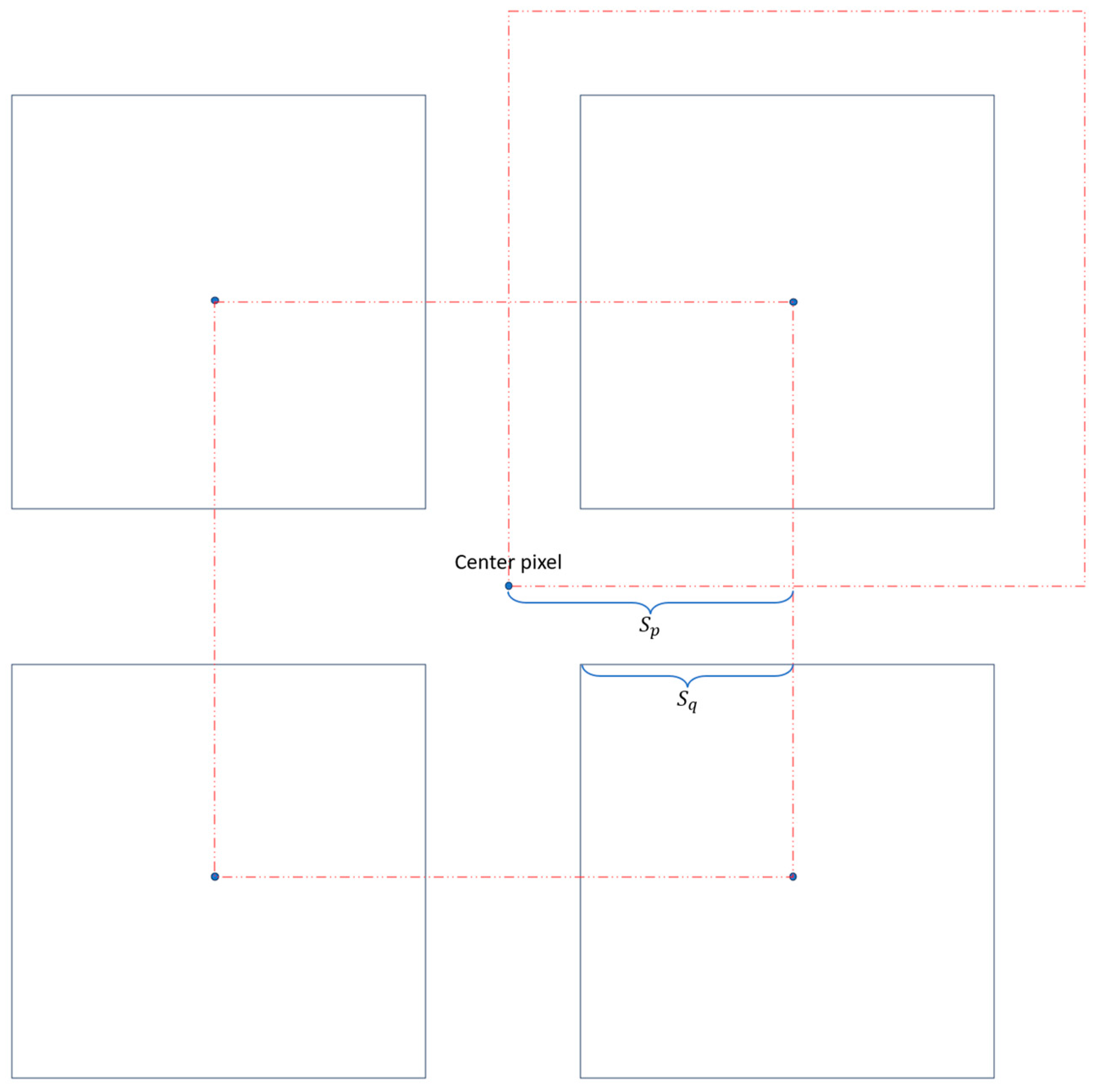
• Novel Edge-Region Detection Method: we propose a new method for detecting edge regions that significantly improves the accuracy of edge localization in blurred images. Unlike existing methods that rely primarily on traditional gradient-based techniques, our method uses a more robust approach based on comparing the gradient magnitude of a central pixel with that of surrounding neighborhood patches. This enables us to effectively identify edge regions, especially in blurred images where traditional methods may struggle. The method places a particular emphasis on aggregating edge regions, allowing for the sufficient detection of both sharp and smoothed edges that may have been affected by blur. This approach is designed to be particularly applicable in real-world scenarios such as infrared imaging, where edges are often blurred but still essential for interpretation.
• Gradient Fusion ($CGF$) Prior Term: based on the edge detection method, we introduce a $CGF$ prior term within the MAP framework, which incorporates the gradient fusion features of image edges. The $CGF$ prior term is specifically designed to exploit the sparse nature of sharp-edge regions in clear images. This sparsity helps alleviate the ill-posed nature of optimization problems typically encountered in image restoration tasks. Notably, the proposed method outperforms existing edge-preserving techniques by providing a more accurate and efficient way to handle blurred regions without over-smoothing important edge details.
• Effective Blur Kernel Estimation with Structural Compensation: in the blur kernel estimation process, we incorporate grayscale values from pixels within the detected edge regions of the blurred image into the intermediate latent image. This approach compensates for subtle structural details lost during the blurring process, ensuring that the final latent image retains more accurate structural information. By preserving edge features more effectively, our method improves the overall accuracy of blur kernel estimation. Moreover, we introduce a weight preservation matrix through nonlinear mapping in the TV model, which preserves critical image details, demonstrating the robustness of our approach. The real-world applicability of this method is evident in its ability to handle complex image structures while delivering high-quality restoration results.

The remainder of this paper is organized as follows. Section 3 presents the $\mathrm{C}GF$ prior term, theoretical validation, and statistical experiments. Section 4 provides a detailed description of the iterative computation process for the proposed prior term and algorithm. Section 5 discusses experimental comparisons with state-of-the-art algorithms, demonstrating the effectiveness of the proposed method. In Section 6, we further analyze and discuss the efficacy of our approach. Finally, Section 7 concludes the paper.

3. Mechanism and Supporting Proof

In this section, we first present the proposed $\mathrm{C}GF$ prior, and then we mathematically demonstrate the theoretical validity of the prior. Ultimately, we empirically validated the effectiveness of the prior term in terms of sparsity and diversity on dataset Jilin-1.

The proposed $\mathrm{C}GF$ prior, based on the fusion of image edge gradient features, arises from observed phenomena, including the increase in the area of edge regions following image blurring, the significant reduction in gradient magnitude due to blur-induced smoothing, and the decrease in gradient direction differences among neighboring pixels. We articulate these observations using the following mathematical formulation:

$$\mathrm{C}GF\left(\mathit{I}\right)\left(x\right)=\left\{\begin{array}{c}\phi \left[H\left(\mathit{I}\right)\left(x\right)\right]\nabla I\left(x\right) if E\left(\mathit{I}\right)\left(x\right)=\mathbf{1}\\ 0 otherwise\end{array}\right.$$

(2)

Let $\mathit{I}$ denote the grayscale image and $x$ represent the pixel position. The operator $E\left(\mathit{I}\right)$ selectively preserves the edge regions of the image by setting non-edge regions to zero, with its detailed mathematical implementation to be explained in Section 4.1. The purpose of $E\left(\mathit{I}\right)$ is to distinguish between the edge and non-edge areas of the image. The matrix $\mathit{H}$ represents the gradient direction differences among pixels. By applying a suitable mapping function $\phi (.)$, the weights in the matrix ensure a significant differentiation between the values of $\mathrm{C}GF\left(\mathit{I}\right)$ in the blurred image and the clear image.

As a consequence of blurring, the edge regions of the blurred image are smoothed by the blur kernel, resulting in a larger area than the edge regions in the original clear image. This phenomenon ensures the sparsity of the prior term. In the subsequent sections, we will provide the derivation and experimental validation of the differences in gradient magnitude and direction between the blur kernel and the clear image in the edge regions. Blurry images, affected by the blur kernel, exhibit smoother gradients and a decrease in gradient values. This characteristic is particularly prominent in the edge regions of the image.

Theorem 1. 

Let ${\mathit{y}}_{\mathit{E}}$ denote the prominent edge regions of the image. For prominent edge regions that are at their widest still narrower than the size of the blur kernel, the following inequality holds:

$$‖\mathit{B}\left({\mathit{y}}_{\mathit{E}}\right)‖\le ‖\mathit{I}\left({\mathit{y}}_{\mathit{E}}\right)‖$$

(3)

Proof of Theorem 1. 

According to Young’s convolution inequality [64], we can infer that

$$\mathit{B}\left(\mathit{y}\right)=\mathit{I}\left(\mathit{y}\right)\ast \mathit{K}$$

(4)

where $\mathit{B}$ represents the blurry image, $\mathit{I}$ represents the clear image, $\mathit{K}$ represents the blur kernel, and * denotes the convolution operation. From this, we have

$$‖\mathit{B}\left({\mathit{y}}_{\mathit{E}}\right)‖=‖\mathit{I}\left({\mathit{y}}_{\mathit{E}}\right)\ast \mathit{K}‖\le ‖\mathit{I}\left({\mathit{y}}_{\mathit{E}}\right)‖\times ‖\mathit{K}‖$$

(5)

From the definition of the blur kernel: $K_i>0$, and $\sum K_i$ = 1, we can deduce that $‖\mathit{K}‖\le$1. Since the prominent edge regions are still narrower than the size of the blur kernel $\mathit{K}$, it follows that

$$‖\mathit{B}\left(\mathit{y}\right)‖=‖\mathit{I}\left(\mathit{y}\right)\ast \mathit{K}\left({\mathit{y}}_{\mathit{E}}\right)‖\le ‖\mathit{I}\left(\mathit{y}\right)‖$$

(6)

The inequality applies to the matrix L-norm, and because the gradient transformation is linear, we can easily deduce that

$$‖\nabla \mathit{B}\left({\mathit{y}}_{\mathit{E}}\right)‖\le ‖\nabla \mathit{I}\left({\mathit{y}}_{\mathit{E}}\right)‖$$

(7)

In general, larger gradient values in the image are concentrated at the edges, with significant increases occurring only in areas with sharp edges. The blur kernel has minimal effect on relatively flat regions in the image, especially in infrared remote-sensing images. Figure 1c,d,k will demonstrate this through experimental evidence. □

Theorem 2. 

Let  $\mathit{H}\left(\mathit{I}\right)\left(\mathit{x}\right)$ represent the gradient direction consistency of the pixels at position  $\mathit{x}$ in the image’s edge regions, where lower values indicate weaker directional consistency. In the prominent edge regions, the following inequality holds:

$${‖\mathit{H}\left(\mathit{I}\right)‖}_1>{‖\mathit{H}\left(\mathit{B}\right)‖}_1$$

(8)

Proof of Theorem 2. 

Let $y=arctan\left(x\right)$ denote the arctangent function. The gradient direction in the edge region of each pixel is computed as

$${\mathit{h}\left(s\right)}_{dir}=\arctan \left({\displaystyle \frac{{\nabla }_y\mathit{u}\left(s\right)}{{\nabla }_x\mathit{u}\left(s\right)}}\right)$$

(9)

where ${\nabla }_{x}u$ and ${\nabla }_{y}u$ are the gradient operators in the horizontal and vertical directions, respectively. ${\mathit{h}\left(s\right)}_{dir}$ represents the gradient direction of the pixel at position $s$, and $\mathit{u}\left(s\right)$ represents the grayscale value at position $s$. The gradient direction of a pixel in the blurry image is given by

$${{\mathit{h}}^{\prime }\left(s\right)}_{dir}=\arctan \left({\displaystyle \frac{{\nabla }_y\left({\mathit{u}}^{\prime }\left(s\right)\right)}{{\nabla }_x\left({\mathit{u}}^{\prime }\left(s\right)\right)}}\right)$$

(10)

where $\mathit{u}\prime \left(s\right)$ is the altered grayscale value due to the blur kernel, expressed as

$${\mathit{u}}^{\prime }\left(s\right)=\sum _{z\in {\Omega }_k}\mathit{u}\left(s+\left[{\displaystyle \frac{a}{2}}\right]-z\right)\mathit{K}\left(\mathit{z}\right)$$

(11)

Here, ${\Omega }_k$ and $a$ represent the domain and size of the blur kernel $\mathit{K}$, and $\left[{\displaystyle \frac{a}{2}}\right]$ denotes rounding. The grayscale value in the blurry image is the weighted sum of the corresponding pixels in the clear image.

Due to the blur kernel’s impact, the gradient direction of the pixel is approximated as

$${\mathit{h}″\left(s\right)}_{dir}=\arctan \left({\displaystyle \frac{{\nabla }_y\mathit{u}″\left(s\right)}{{\nabla }_x\mathit{u}″\left(s\right)}}\right)$$

(12)

There is an overlap between the values of ${\mathit{u}}^{\prime }\left(s\right)$ for neighboring pixels and the central pixel. Let us denote this overlapping part as $\mathit{u}\prime \prime \left(s\right)$, which represents the weighted sum of the central and neighboring pixel values, defined as

$$\mathit{u}″\left(s\right)=\sum _{z\in {\Omega }_{k1}\cap {\Omega }_{k2}}\mathit{u}\left(s+\left[{\displaystyle \frac{a}{2}}\right]-z\right)\min \left\{{\mathit{K}}_1\left(\mathit{z}\right),{\mathit{K}}_2\left(\mathit{z}\right)\right\}$$

(13)

The impact of remote-sensing imaging can be approximated by convolving with a circular blur kernel, resulting in a smoothing effect on edge regions. The gradient magnitude, perpendicular to the edge texture region, resembles a “slope”, with gradient directions aligning across neighboring pixels. In contrast, gradient directions in a clear image exhibit more variation. The following equations illustrate this:

$${‖\mathit{H}\left(\mathit{I}\right)‖}_1>{‖\mathit{H}\left(\mathit{B}\right)‖}_1$$

(14)

$$\mathit{s}.\mathit{t}.\mathit{H}\left(\mathit{I}\right)\left(s\right)=\left|{\displaystyle \frac{1}{N}}\sum _{\begin{array}{c}z\in {\Omega }_s\end{array}}{\mathit{h}\left(z\right)}_{dir}-{\mathit{h}\left(s\right)}_{dir}\right|$$

$N$ represents the number of pixels in the neighborhood ${\Omega }_s$. The neighborhood region does not include the central pixel, i.e., $s\notin {\Omega }_s,{\Omega }_s$ In experiments, the choice of a four-neighborhood or an eight-neighborhood is expected. □

The above theory can be experimentally validated in Figure 1e,f,l:

The theoretical analysis and experimental results demonstrate significant differences between blurry and clear images regarding gradient magnitude and direction in the edge regions. The edge regions of clear images tend to be sharper and more concentrated. In contrast, the edge regions of blurry images are influenced more by the blur kernel, and have a wider distribution. A new deblurring model is proposed based on the MAP framework by focusing on the comprehensive differences between blurry and clear images in terms of edge region size, gradient magnitude, and gradient direction.

The main flow chart of the algorithm in this paper is as follows: the flowchart of Figure 2 corresponds to the process of establishing the prior term, as described in Section 4.2 of the paper. The middle flowchart represents the main algorithm for solving the latent image and the blur kernel, corresponding to Section 4.3.1 and Section 4.3.2 The bottom flowchart illustrates the algorithm for restoring the image, corresponding to Section 4.3.3 of the paper.

4. The Blind Deconvolution Model and Optimization

Based on the introduction above and the analysis, a novel blind deblurring model is proposed. This section will primarily introduce the mathematical linearization of the prior term, along with the algorithm’s detailed computations and iterative process.

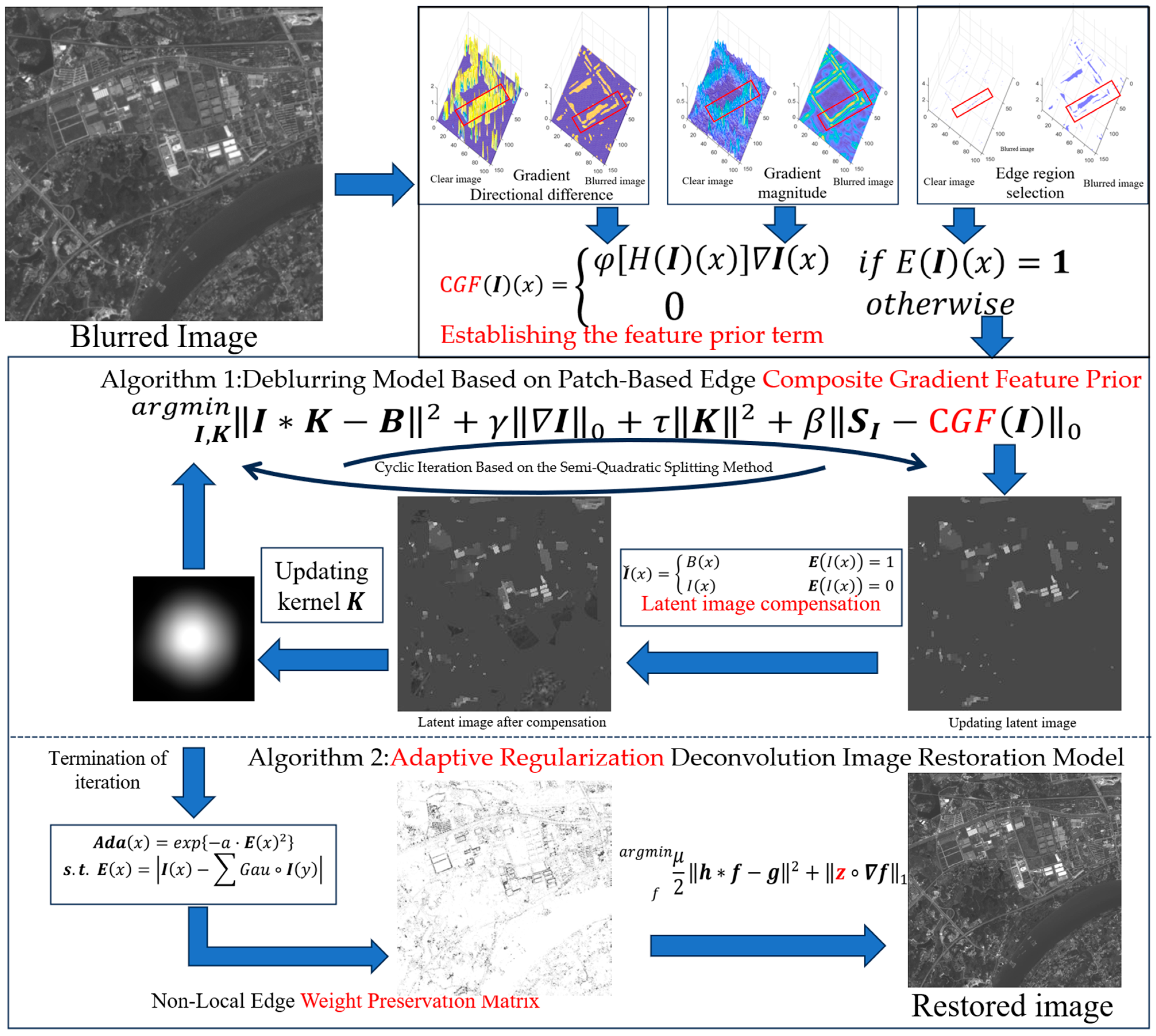
4.1. Patch-Based Edge Composite-Gradient Feature Prior and Deblurring Model

Within the conventional MAP framework, the blind deblurring model is defined as follows:

$${}_{\mathit{I},\mathit{K}}{}^{argmin}{‖\mathit{I}\ast \mathit{K}-\mathit{B}‖}^2+\gamma {‖\nabla \mathit{I}‖}_0+\tau {‖\mathit{K}‖}^2+\beta {‖{\mathit{S}}_{\mathit{I}}-\mathrm{C}GF\left(\mathit{I}\right)‖}_0$$

(15)

β, γ, and τ are weighting parameters corresponding to the following regularization terms. The first fidelity term strengthens the similarity between the convolution result $\mathit{I}\ast \mathit{K}$ and the observed blurry image $\mathit{B}$. The second term ensures that only salient edges affect the function, by removing tiny ones introduced in [28] and those previously used combined in [41,42,43,44,45,46,47]. The regularization term for the third term is applied to the blur kernel. For computational convenience, we employ the conventional L2 norm in the calculations, which constrains the smoothness of the kernel. The fourth term is the previously mentioned term based on the fusion of image edge gradients. Minimizing this term ensures that the algorithm prefers clear images rather than blurry ones. The prior term is optimized using an approximate L0 norm regularization, and we will now introduce the mathematical implementation of this prior term.

4.2. Implementation of $CGF$ Prior, Mathematically

Before presenting the algorithmic computation process, we address a tricky problem associated with the operation of the $\mathrm{C}GF$ prior term:

$${\mathit{A}}_{\mathit{h}}\left(x\right)=\left\{\begin{array}{c}1, {\nabla \mathit{I}}_{\mathit{h}}\left(x\right)>0\\ -1, {\nabla \mathit{I}}_{\mathit{h}}\left(x\right)<0 \end{array}\right.$$

(16)

Similar to ${\mathit{A}}_{\mathit{v}}$, we have

$$\left|\nabla \mathit{I}\right|=\mathit{A}\odot \nabla \mathit{I}$$

(17)

Here, we use ⊙ to denote the Hadamard product. Note that the gradient operator ∇ involves two directions, i.e., $\nabla =({\nabla }_x,{\nabla }_y)$, where ${\nabla }_x$ and ${\nabla }_y$ represent the horizontal and vertical directions, respectively. Similarly, the corresponding absolute operator is also applied in both directions, i.e., $A=(A_x,A_y)$. It is important to note that in the vector form of $I$, both operators $A$ and $\nabla$ are sparse. In this case:

$$\left|\nabla \mathit{I}\right|=\mathit{A}\nabla {\mathit{I}}^1$$

(18)

4.2.1. Edge Region Selection Operator

Inspired by [41,46], we replace the edge detection operator with a sparse matrix E, applied to the vectorized form of |∇I|. By traversing two types of patches, we achieve the effect of edge detection. This method effectively captures the difference in edge region areas in L0 norm sparsity between clear and blurry images in the prior term.

$$\mathit{E}\left(\mathit{I}\right)\left(x\right)=\left\{\begin{array}{c}1, \nabla \left(\mathit{I}\right)\left(x\right)\ge Min\left(Max\left(\nabla {\mathit{I}\left(x\right)}_Y\right)\right) \\ 0, otherwise \end{array}\right.$$

(19)

${I\left(x\right)}_Y$ denotes a collection of multiple-gradient patch matrices centered around each neighboring pixel of $I\left(x\right)$. For each patch matrix in ${I\left(x\right)}_Y$, the corresponding gradient values $\left|\nabla {I\left(x\right)}_Y\right|$ are further computed to determine the maximum value among each gradient patch of ${I\left(x\right)}_Y$, $Max(\nabla {I\left(x\right)}_Y).$ Then $Min\left(Max\left(\nabla {I\left(x\right)}_Y\right)\right)$ represents the minimum value in this set of maximum gradient values $Max(\nabla {I\left(x\right)}_Y$. If the gradient of the central pixel is greater than the maximum gradient of any surrounding neighborhood block ${I\left(x\right)}_Y$, the pixel is considered part of the edge region

The patch size of the pixel neighborhood is denoted as $S_p$, and the patch size used to compute the maximum gradient value for each patch is denoted as $S_q$. As shown in Figure 3, when $S_q$ remains constant, a larger $S_p$ makes classifying a pixel as an edge pixel easier. When $S_p$ = $S_q$, the maximum value pixel for each patch is preserved. A smaller $S_p$ imposes a stricter requirement for the central pixel to be classified as an edge pixel. When $S_p$ is small enough (e.g., 0), there is only one matrix in ${I\left(x\right)}_Y$, and in this case, the central element is selected if it represents the gradient extremum within a window of size $S_q$. This reasoning can be summarized as follows:

Let us assume $S_{p1}<S_{p2}$. We refer to the matrix collection corresponding to $S_{p1}$ as $I_{Y1}$ and the matrix collection corresponding to $S_{p2}$ as $I_{Y2}$. Additionally, we denote the set of matrices in $I_{Y2}$, excluding $I_{Y1}$, as $I_{Y\prime }$. This can be represented as follows:

$$Min\left(Max(\nabla {\mathit{I}}_{Y2}\right))=Min\left(Max(\nabla {\mathit{I}}_{Y1}\right),Max(\nabla {\mathit{I}}_{Y^{\prime }}\left)\right)$$

(20)

• If $Max\left(\nabla I_{Y^{\prime }}\right)\ge Max(\nabla I_{Y1})$, then $Min\left(Max(\nabla I_{Y2}\right))=Min(Max(\nabla I_{Y1}))$
• If $Max\left(\nabla {\mathit{I}}_{Y^{\prime }}\right)<Max(\nabla {\mathit{I}}_{Y1})$, then $Min$(Max($\nabla {\mathit{I}}_{Y2}$))= $Min\left(Max\right(\nabla I_{Y\prime }\left)\right)$ 

In conclusion, we have: $Min\left(Max(\nabla {\mathit{I}}_{Y1}\right),Max(\nabla {\mathit{I}}_{Y^{\prime }}))\le Min(Max(\nabla {\mathit{I}}_{Y1}))$; that is

$$Min\left(Max\left(\nabla {\mathit{I}}_{Y2}\right)\right)\le Min\left(Max\left(\nabla {\mathit{I}}_{Y1}\right)\right)$$

(21)

Alternatively, it can be expressed as

$${\mathit{E}}_{S_{p2}}\left(\mathit{I}\right)\left(x\right)\ge {\mathit{E}}_{S_{p1}}\left(\mathit{I}\right)\left(x\right)$$

(22)

Therefore, in the experiments, choosing the patch size for the gradient patch and the patch size for the pixel neighborhood controls the extent of edge preservation.

Sparsity of ${\mathit{L}}_0-\mathit{n}\mathit{o}\mathit{r}\mathit{m}$: the fundamental concept behind $\mathit{E}\left(I\right)$ is to selectively preserve pixels by comparing the gradient of the central pixel with the maximum gradient values of surrounding patches. In clear images, edges are more defined, and the edge regions are highly concentrated. However, the blurring kernel expands sharp-edge regions into broader, less-sharp areas in the blurred image. Consequently, when $S_q$ and $S_p$ remaining constant, the maximum gradient values obtained from multiple gradient patches of ${\nabla \mathit{I}\left(x\right)}_Y$ often originate from the same pixel, with a more enormous gradient value than blurred images. Consequently, the selected pixels are exclusively from more vital edge regions. In contrast, in blurry images, the gradients of image edges are smoothed, and the previously larger gradient values are distributed over a more extensive area. Consequently, adjacent gradient patches in the smoothed-edge region consistently obtain different maximum edge gradient values. This results in the preservation of more edge pixels.

4.2.2. Quantification of Gradient Direction Differences in Edge Regions

As described in Equation (14), the gradient directional difference function $\mathit{H}\left(\mathit{I}\right)\left(s\right)$ calculates the difference between ${h\left(s\right)}_{dir}$ and the mean value of the neighboring pixels, effectively forming the gradient directional difference matrix. An appropriate normalization mapping function can amplify the differences in the L-norms of the prior terms between sharp and blurred images, thereby accelerating the convergence of the computation. The currently selected mapping function consists of three conditions:

• The chosen mapping function, $\phi (.)$, is a non-negative and increasing function;
• The function $\phi (.)$ is designed to have small increments at the two ends and larger increments in the middle;
•  $\phi \left(.\right){lim}_{H\to H_{min}}\phi \left(H\right)=0$ and ${lim}_{H\to H_{max}}\phi \left(H\right)=1$. Among them, $H_{min}$ and $H_{max}$ are the minimum and maximum values of the Gradient Direction Difference Matrix $H$, respectively.

This paper assumes that the standard ‘sigmoid’ function satisfies the above requirements, but the scale and phase of σ(x) must be adjusted. Therefore, the mapping function $\phi (\cdot )$ can be expressed as

$$\phi \left(\mathit{H}\left(\mathit{I}\right)\left(s\right)\right)={\displaystyle \frac{1}{1+e^{-k\left(\mathit{H}\left(\mathit{I}\right)\left(s\right)-m\right)}}}$$

(23)

$$s.t. m={\displaystyle \frac{\lambda }{N}}\sum _{i=1}^N\mathit{H}\left(\mathit{I}\right)\left(s\right)$$

(24)

Figure 4 illustrates the variations in the information components of the $\mathrm{C}GF$ prior term before and after the blurring process.

4.2.3. The Implementation of the Calculation of $CGF\left(\mathit{I}\right)$ Prior Term

All the matrices could be acquired during the deblurring process. The calculations are performed using an intermediate latent image. Let $\mathit{P}=\mathit{E}\ast \mathit{A}\ast \mathit{F}\ast \nabla ,$ then $\mathit{P}\mathit{G}\mathit{F}$ operation can be written as

$$\mathrm{C}GF\left(\mathit{I}\right)=\mathit{E}\ast \mathit{A}\ast \mathit{F}\ast \nabla \mathit{I}=\mathit{P}\mathit{I}$$

(25)

In matrix $\mathit{P}$, all matrices are transformed Toeplitz sparse matrices, and $\mathit{I}$ represents the vectorized degraded image. Both the L0 norm and L1 norm of the prior term exhibit significant improvements, as shown in Figure 1i,j:

$${‖\mathrm{C}GF\left(\mathit{I}\right)‖}_{\mathbf{0}}<{‖\mathrm{C}GF\left(\mathit{B}\right)‖}_{\mathbf{0}}$$

(26)

Direct implementation of L0 norm regularization is challenging. To enhance the sparsity prior of the ideal image in the prior term, the ${\mathit{S}}_{\mathit{I}}$ term is introduced. This regularization term not only captures the inherent sparsity differences in the L0 norm, but also highlights the significant distinctions between the L1 and L2 norms for clear and blurry images.

$${‖{\mathit{S}}_{\mathit{I}}-\mathrm{C}GF\left(\mathit{I}\right)‖}_{\mathbf{0}}<{‖{\mathit{S}}_{\mathit{B}}-\mathrm{C}GF\left(\mathit{B}\right)‖}_{\mathbf{0}}$$

(27)

$$s.t. {\mathit{S}}_{\mathit{I}}=\left\{\begin{array}{c}{\displaystyle \frac{\mathit{d}}{\mathbf{m}\mathbf{a}\mathbf{x}\left(\mathit{P}\mathit{I}\right)}} PI>0\\ 0, otherwise\end{array}\right.$$

(28)

The ${\mathit{S}}_{\mathit{I}}$ matrix is structured as a sparse matrix corresponding to the gradient feature prior term $\mathrm{C}GF\left(\mathit{I}\right)$, with $\mathit{d}$ defined as the square of the maximum theoretical value of $\mathit{P}\mathit{I}$, adjusted by gradient operators. Initially, when the image is highly blurred, $\mathit{P}\mathit{I}$ is low, resulting in larger values for the non-zero elements in ${\mathit{S}}_{\mathit{I}}$. As the latent image clarifies through iterations, $\mathrm{m}\mathrm{a}\mathrm{x}\left(\mathit{P}\mathit{I}\right)$ increases, aligning ${\mathit{S}}_{\mathit{I}}$ with clear image values and enhancing the sparsity of the prior terms. The L1 norm is a convex relaxation of the L0 norm, improving sparse representation. Compared to LMG and DCP [41,44], our method uses a prior term with enhanced discriminative ability and sparsity, updated throughout the iterations.

4.3. Model and Optimization

Rather than directly optimizing the Function (15), the energy function is decomposed into two sub-problems, and alternating optimization iterations are implemented. The two sub-problems can be formulated as follows:

$${}_{\mathit{I}}{}^{min}{‖\mathit{I}\ast \mathit{K}-\mathit{B}‖}^2+\gamma {‖\nabla \mathit{I}‖}_0+\beta {‖{\mathit{S}}_{\mathit{I}}-\mathrm{C}GF\left(\mathit{I}\right)‖}_0$$

(29)

$${}_{\mathit{K}}{}^{min}{‖\mathit{I}\ast \mathit{K}-\mathit{B}‖}^2+\tau {‖\mathit{K}‖}^2$$

(30)

4.3.1. Optimization of Intermediate Latent Image

To estimate the latent image:

$${}_{\mathit{I}}{}^{min}{‖\mathit{I}\ast \mathit{K}-\mathit{B}‖}^2+\gamma {‖\nabla \mathit{I}‖}_0+\beta {‖{\mathit{S}}_{\mathit{I}}-\mathrm{C}GF\left(\mathit{I}\right)‖}_0$$

(31)

Due to the non-convex nature of the L0 norm, direct optimization of Equation (31) becomes computationally challenging. Thus, a semi-quadratic splitting method is employed [27]; replace $\mathit{u}$ with ${\mathit{S}}_{\mathit{I}}-\mathrm{C}GF\left(\mathit{I}\right)$, and $\mathit{g}$ with $\nabla \mathit{I}$.

$$\begin{array}{c}{}_{\mathit{I},\mathit{u},\mathit{g}}{}^{min}{‖\mathit{I}\ast \mathit{K}-\mathit{B}‖}_{\mathbf{2}}^{\mathbf{2}}+\beta {‖\mathit{u}‖}_0+\gamma {‖\mathit{g}‖}_{\mathbf{0}}+\\ {\alpha }_1{‖{\mathit{S}}_{\mathit{I}}-\mathrm{C}GF\left(\mathit{I}\right)-\mathit{u}‖}^{\mathbf{2}}+{\alpha }_2{‖\nabla \mathit{I}-\mathit{g}‖}^{\mathbf{2}}\end{array}$$

(32)

here, ${\alpha }_1$ and ${\alpha }_2$ are penalty parameters, and the solution is obtained through alternating optimization of $\mathit{I}$, $\mathit{u}$, and $\mathit{g}$. Given the prior matrix $\mathit{P},$ the lead to $\mathit{P}\mathit{I}=\mathrm{C}GF\left(\mathit{I}\right)$. The solution for $\mathit{I}$ can be obtained through the following approach:

$${}_{\mathit{I}}{}^{min}{‖\mathit{K}\mathit{I}-\mathit{B}‖}^2+{\alpha }_1{‖{\mathit{S}}_{\mathit{I}}-\mathit{P}\mathit{I}-\mathit{u}‖}^2+{\alpha }_2{‖\nabla \mathit{I}-\mathit{g}‖}^2$$

(33)

here, we use $\mathit{K}$ to denote the Toeplitz form of blur kernel $\mathit{K}$, $\mathit{B}$, $\mathit{u}$, $\mathit{g}$ to denote the vector form of $\mathit{B}$,$\mathit{u}$, $\mathit{g}$, respectively.

Equation (32) is the quadratic problem for $\mathit{I}$, which can be solved using the conjugate gradient (CG) method. However, since Equation (32) involves a large-size matrix $\mathit{P}$, the CG method requires significant computational labor. Similar to earlier studies [44,46], we achieve equilibrium between accuracy and speed by introducing another variable $\mathit{q}$, which corresponds to $\mathit{I}$.

$$\begin{array}{c}{}_{\mathit{I},\mathit{q}}{}^{min}{‖\mathit{K}\mathit{I}-\mathit{B}‖}^2+{\alpha }_1{‖{\mathit{S}}_{\mathit{I}}-\mathit{P}\mathit{q}-\mathit{u}‖}^2+\\ {\alpha }_2{‖\nabla \mathit{I}-\mathit{g}‖}^2+{\alpha }_3{‖\mathit{I}-\mathit{q}‖}^{\mathbf{2}}\end{array}$$

(34)

where ${\alpha }_3$ is a positive penalty parameter. We can solve Equation (34) by updating $\mathit{I}$ and $\mathit{q}$ in an alternative manner, which is given by

$${}_{\mathit{I}}{}^{min}{‖\mathit{K}\mathit{I}-\mathit{B}‖}^2+{\alpha }_2{‖\nabla \mathit{I}-\mathit{g}‖}^2+{\alpha }_3{‖\mathit{I}-\mathit{q}‖}^2$$

(35)

$${}_{\mathit{q}}{}^{min}{\alpha }_1{‖{\mathit{S}}_{\mathit{I}}-\mathit{P}\mathit{q}-\mathit{u}‖}^2+{\alpha }_3{‖\mathit{I}-\mathit{q}‖}^2$$

(36)

The two equations have closed-form solutions, solved by FFT for Equation (34).

$$\mathit{I}=F^{-1}{\displaystyle \frac{\overline{F\left(\mathit{K}\right)}F\left(\mathit{B}\right)+{\alpha }_2\overline{F\left(\nabla \right)}F\left(\mathit{g}\right)+{\alpha }_{3}F\left(\mathit{q}\right)}{\overline{F\left(\mathit{K}\right)}F\left(\mathit{K}\right)+{\alpha }_2\overline{F\left(\nabla \right)}F\left(\nabla \right)+{\alpha }_3}}$$

(37)

where $F(\cdot )$ and $F^{-1}(\cdot )$ represent FFT and inverse FFT, respectively, and F(⋅) represents a complex conjugate operator. Equation (36) can be obtained directly, using the following Equation:

$$\mathit{q}={\displaystyle \frac{{\alpha }_1{\mathit{P}}^{\mathit{T}}\left({\mathit{S}}_{\mathit{I}}-\mathit{u}\right)+{\alpha }_3\mathit{I}}{{\alpha }_1{\mathit{P}}^{\mathit{T}}\mathit{P}+{\alpha }_3}}$$

(38)

Given I, we can compute u and g separately by following two sub-equations:

$${}_{\mathit{u}}{}^{min}{\beta ‖\mathit{u}‖}_0+{\alpha }_1{‖{\mathit{S}}_{\mathit{I}}-\mathit{P}\mathit{I}-\mathit{u}‖}^2$$

(39)

$${}_{\mathit{g}}{}^{min}\gamma {‖\mathit{g}‖}_0+{\alpha }_2{‖\nabla \mathit{I}-\mathit{g}‖}^2$$

(40)

The above formulas are both pixel-wise minimization problems, which can be solved directly by [28]. We obtain the iterations of $\mathit{u}$ and $\mathit{g}$ as follows:

$$\mathit{u}=\left\{\begin{array}{c}{\mathit{S}}_{\mathit{I}}-PI, {\left|{\mathit{S}}_{\mathit{I}}-\mathit{P}\mathit{I}\right|}^{\mathbf{2}}\ge {\displaystyle \frac{\beta }{{\alpha }_1}}\\ \mathbf{0}, \mathit{o}\mathit{t}\mathit{h}\mathit{e}\mathit{r}\mathit{w}\mathit{i}\mathit{s}\mathit{e}\end{array}\right.$$

(41)

$$\mathit{g}=\left\{\begin{array}{c}\nabla u, {\left|\nabla \mathit{I}\right|}^2\ge {\displaystyle \frac{\gamma }{{\alpha }_2}}\\ \mathbf{0}, \mathit{otherwise}\end{array}\right.$$

(42)

The procedure of Algorithm 1 is as follows.

Algorithm 1 Calculate intermediate latent Image

Input: blurred image $\mathit{B}$, blur kernel $k$          For i = 1:5 do          Compute matrix $\mathit{P}$ using (25).          Compute matrix ${\mathit{S}}_{\mathit{I}}$ using (28).          For i = j:4 do                  Compute matrix $\mathit{q}$ using (38).                            ${\alpha }_2=2{\alpha }_2$.                                  repeat                                        Compute matrix $\mathit{I}$ using (37).                                        ${\alpha }_2=k\ast {\alpha }_2$.                                  until ${\alpha }_2>max {\alpha }_2$                                                                            ${\alpha }_3=4{\alpha }_3$                  End for                                                                                  ${\alpha }_1=4{\alpha }_1$          End for          Output: Intermediate latent Image $\mathit{I}$.

4.3.2. Estimating Blur Kernel $\mathit{K}$

To estimate the blur kernel and restore a clear image, prior models reveal that the L0 term ${‖\nabla \mathit{I}‖}_0$ is a more effective deblurring regularizer than the L1 term ${‖\nabla \mathit{I}‖}_1$, significantly outperforming it in reducing blur. ${‖\nabla \mathit{I}‖}_0$ regularizes the latent image $\mathit{I}$ into a piecewise function, preserving major structural elements while smoothing some edges. To recover these smoothed edges, spatial information from edge pixels in the prior term $\mathrm{C}GF\left(\mathit{I}\right)$ is used to supplement missing details. The gradient values of pixels selected by $\mathit{E}\left(\mathit{I}\right)$ are strongly influenced by the blur kernel, corresponding to fine edge details. Thus, grayscale values from corresponding positions in the previous blurred image are reassigned to the latent image, compensating for edge detail loss and enhancing the next-level $\mathrm{C}GF\left(\mathit{I}\right)$ prior calculation, as illustrated in Figure 5. In the region marked by the red circle in the figure, it is evident that the latent-image details processed by our algorithm exhibit richer textures, thereby enhancing the accuracy of the blur kernel.

$$\check{\mathit{I}}\left(x\right)=\left\{\begin{array}{c}B\left(x\right) \mathit{E}\left(I\left(x\right)\right)=1\\ I\left(x\right) \mathit{E}\left(I\left(x\right)\right)=0 \end{array}\right.$$

(43)

Solving the blur kernel model:

$${}_{\mathit{k}}{}^{min}{‖\mathit{k}\ast \nabla \check{\mathit{I}}-\nabla \mathit{B}‖}_2^2+\gamma {‖\mathit{k}‖}_2^2$$

(44)

The formula to be solved is

$$\mathit{k}=F^{-1}\left({\displaystyle \frac{\overline{F\left(\nabla \check{\mathit{I}}\right)}F\left(\nabla \mathit{B}\right)}{\overline{F\left(\nabla \check{\mathit{I}}\right)}F\left(\nabla \mathit{B}\right)+\gamma }}\right)$$

(45)

Similar to existing advanced methods [30,41,46], a multiscale strategy from coarse to fine based on image pyramids is employed in terms of the specific implementation. Additionally, when obtaining $\mathit{k}$, the negative elements of $\mathit{k}$ are set to 0 and normalized to meet the definition of the kernel.

4.3.3. Restore Clear Image by Adaptive Regularization Model

In infrared remote-sensing images, the grayscale characteristics of pixels in large background areas often appear relatively flat, with only a tiny portion containing valuable information. Therefore, based on the traditional TV model of non-blind deconvolution, adaptive weight assignment is applied to the smoothness preservation term ${‖\nabla \mathit{f}‖}_1$. After estimating the blur kernel using an enhanced intermediate latent image $\check{\mathit{I}}\left(x\right)$ with detailed features, the blur kernel K becomes more accurate, balancing overall image smoothing and preserving edge details. Following the kernel estimation stage, the restoration of the blurred image enters the second phase, where we introduce a weighted preservation matrix for detail regions into the smoothness term $‖\nabla \mathit{f}‖$. Utilizing a detail weight preservation matrix based on grayscale differences, we use the more accurate blur kernel obtained from the solution. $\check{\mathit{I}}\left(x\right)$ to recover the image. Consequently, the grayscale discontinuity introduced by the intermediate latent image in the first phase does not propagate to the second phase, thereby influencing the final quality of the recovered image:

$${}_f{}^{argmin}{\displaystyle \frac{\mu }{2}}{‖\mathit{h}\ast \mathit{f}-\mathit{g}‖}^2+{‖\mathit{z}\circ \nabla \mathit{f}‖}_1$$

(46)

where $\mathit{h}$ is the kernel of acquired $\mathit{K}$, $\mathit{f}$ is the recovered image to be solved, $\mathit{g}$ is the original blurred image, and $\mathit{z}$ is the regularization weight-mapping matrix, $\circ$ representing the Hadamard inner product between matrices. To address the problem involving both convolution and Hadamard terms, we vectorize the matrices and transform the convolution and Hadamard products into sparse matrix multiplication for the solution

$${}_f{}^{min}{\displaystyle \frac{\mu }{2}}{‖\mathit{H}·\overrightarrow{\mathit{f}}-\overrightarrow{\mathit{g}}‖}^2+{‖\mathit{Z}·\mathit{G}·\overrightarrow{\mathit{f}}‖}_1$$

(47)

where $\overrightarrow{\mathit{f}}$ and $\overrightarrow{\mathit{g}}$ are vectorized forms of the original image matrix, while $\mathit{H}$, $\mathit{Z},$ and $\mathit{G}$ are Toeplitz sparse matrices. $\mathit{G}$ is the sparse matrix of the operator $\nabla$. To address this issue, we introduce the parameter $\overrightarrow{\mathit{Q}}=\mathit{Z}·\mathit{G}·\overrightarrow{\mathit{f}}$. Then the problem is transformed to

$${}_{\mathit{f},\mathit{Q}}{}^{min}{\displaystyle \frac{\mu }{2}}{‖\mathit{H}·\overrightarrow{\mathit{f}}-\overrightarrow{\mathit{g}}‖}^2+{‖\overrightarrow{\mathit{Q}}‖}_1+\mathsf{\lambda }{‖\overrightarrow{\mathit{Q}}-\mathit{Z}·\mathit{G}·\overrightarrow{\mathit{f}}‖}_2^2$$

(48)

For subproblem $\overrightarrow{Q}$:

$${}_{\mathit{Q} }{}^{min}{‖\overrightarrow{\mathit{Q}}‖}_1+\mathsf{\lambda }{‖\overrightarrow{\mathit{Q}}-\mathit{Z}·\mathit{G}·\overrightarrow{\mathit{f}}‖}_2^2$$

(49)

Solved as:

$$\overrightarrow{\mathit{Q}}=sign(\mathit{Z}·\mathit{G}·\overrightarrow{\mathit{f}})·\mathrm{m}\mathrm{a}\mathrm{x}(\left|\mathit{Z}·\mathit{G}·\overrightarrow{\mathit{f}}\right|-{\displaystyle \frac{\mathit{\lambda }}{2}},\mathbf{0})$$

(50)

For subproblem $\overrightarrow{\mathit{f}}$:

$${}_{\mathit{f}}{}^{\mathit{m}\mathit{i}\mathit{n}}{\displaystyle \frac{\mathit{\mu }}{2}}{‖\mathit{H}·\overrightarrow{\mathit{f}}-\overrightarrow{\mathit{g}}‖}^2+\mathit{\lambda }{‖\mathit{Q}-\mathit{Z}·\mathit{G}·\overrightarrow{\mathit{f}}‖}_2^2$$

(51)

Solved as:

$$\overrightarrow{\mathit{f}}={\displaystyle \frac{\mu {\mathit{H}}^{\mathit{T}}\overrightarrow{\mathit{g}}+2\mathsf{\lambda }{\left(\mathit{Z}·\mathit{G}\right)}^{\mathit{T}}·\mathit{Q}}{\mu {\mathit{H}}^{\mathit{T}}·\mathit{H}+2\mathsf{\lambda }{\left(\mathit{Z}·\mathit{G}\right)}^{\mathit{T}}·\mathit{Z}·\mathit{G}}}$$

(52)

Here, $\mathit{G}$ represents an operator that computes the gradients in both the $x$ and $y$ directions. For subproblem $\mathit{z}$, to ensure the pixel gradients in important edge regions, the weight matrix is set as follows, where $Gau$ represents the Gaussian fuzzy kernel and $a$ represents the parameter.

$$\mathit{Z}\left(x\right)=\mathit{exp}\left\{-a{·\mathit{E}\left(x\right)}^2\right\}$$

(53)

$$\mathit{s}.\mathit{t}. \mathit{E}\left(x\right)=\left|\mathit{I}\left(x\right)-\sum Gau\circ \mathit{I}\left(y\right)\right|$$

(54)

The proposed detail-weighted regularization matrix ensures the continuity of the image structure. Unlike edge detection methods that binarize weights into high and low values, this approach better preserves the overall structural integrity of the image and demonstrates greater robustness. Combined with the previously compensated blur kernel, it facilitates the recovery of a more accurate and precise image.The procedure of Algorithm 2 is as follows.

Algorithm 2 Estimating blur kernel $\mathit{K}$ and restore clear Image

Input: blurred Image $\mathit{B}$, Intermediate latent Image $\mathit{I}$ Initialize $\mathit{K}$ from the previous layer of the pyramid. While i < maxiter do              Estimate $k$ according to (45)                    Compensation of detail through (43) End While Set parameters $a$ (default = 2) and $\mu$ (default = 0.7). Initialize $\mathit{f}=\mathit{B}$, $\mathit{z}=1.$ while not converging, do 1. Solve the $\overrightarrow{\mathit{Q}}$-subproblem (49) using (50). 2. Solve the $\overrightarrow{\mathit{f}}$-subproblem (51) using (52). 3. Update the weight matrix $\mathit{z}$ using (53). if ${\displaystyle \frac{{‖{\mathit{f}}_{\mathit{k}+1}-{\mathit{f}}_{\mathit{k}}‖}_2}{{‖{\mathit{f}}_{\mathit{k}}‖}_2}}\le tol$ then break end if break Output: Clear image $\mathit{f}$.

5. Numerical Experiments

To verify the processing performance of the proposed method, high-resolution remote-sensing images such as “Jilin-1”, “Pleiades”, and “WorldView-3” were selected as real scenes. An image quality-degradation model (simulated conditions based on the parameters of the “Jilin-1” satellite) was employed to simulate degraded images. To simulate various degradation scenarios for the images, we applied convolutional blur using Gaussian kernels of different sizes and variances. Subsequently, the remote-sensing dataset with images sized at 1024 × 1024 pixels was obtained through image cropping. In order to thoroughly compare the competitiveness of the algorithm, the degradation features of each image are different. Next, various prior algorithms and the proposed method in this paper were applied to deblur the degraded images. The other methods used a unified traditional TV model deconvolution after estimating the blur kernel [10].

Various factors influencing on-orbit imaging tend to be uniform in direction, particularly with defocus blur being predominant. The literature estimates blur kernels for multiple remote-sensing images, with the estimated blur kernels primarily being circular or approximately circular [65]. The size of the blur kernel reflects the severity of the blur. Consequently, this paper employs Gaussian blur kernels of different sizes to degrade the images. By setting the standard deviation of the blur kernel, the degree of blur degradation can be controlled, thus achieving directionally uniform degradation in remote-sensing images. The shapes of the blur kernels are all circular.

To evaluate the image quality before and after processing, we selected the structural similarity index (SSIM), visual information fidelity (VIF), peak signal-to-noise ratio (PSNR), DE [66],EME [67], and NIQE [68]. The SSIM index evaluates the restoration capability of scene edges and texture details, and can be expressed as

$$SSIM={\displaystyle \frac{2\left({\mu }_x{\mu }_y+C_1\right)\left(2{\sigma }_{xy}+C_2\right)}{\left({{\mu }_x}^2+{{\mu }_y}^2+C_1\right)\left({{\sigma }_x}^2+{{\sigma }_y}^2+C_2\right)}}$$

(55)

where, ${\mu }_x,{\mu }_y$ and ${{\sigma }_x}^2$, ${{\sigma }_y}^2$ are the mean and variance of the two images, respectively ${\sigma }_{xy}$ is the covariance, $C_1$ and $C_2$ are adjustable parameters. VIF is used to evaluate the ability of an algorithm to improve the scene definition and vision effect. The calculation formula is given by

$$VIF={\displaystyle \frac{I({\overrightarrow{C}}^N;{\overrightarrow{E}}^N|s^N)}{I({\overrightarrow{C}}^N;{\overrightarrow{F}}^N|s^N)}}$$

(56)

where $I({\overrightarrow{C}}^N;{\overrightarrow{E}}^N|s^N)$ and $I({\overrightarrow{C}}^N;{\overrightarrow{F}}^N|s^N)$ represent the information that the brain can ideally extract from the reference and impaired images, respectively. As described below, the signal-to-noise ratio SNR can evaluate the ability of an algorithm to suppress noise and artifacts.

$$PSNR=10\times \lg \left[{\displaystyle \frac{{{MAX}^2}_I}{\frac{1}{mn}{\sum }_{i=0}^{m-1}{\sum }_{j=0}^{n-1}{\left(I\left(i,j\right)-K\left(i,j\right)\right)}^2}}\right]$$

(57)

where ${MAX}_I$ represents the possible maximum pixel value in the image, and $m$ and $n$ are the numbers of rows and columns in the image, respectively. $I(i,j)$ and $K(i,j)$ denote the pixel values at the position $(i,j)$ in the original and processed images. PSNR is measured in decibels (dB), representing the logarithmic scale of the signal-to-noise ratio. A higher PSNR value indicates a more significant similarity between the two images, implying better quality in the processed image.

5.1. Experimental Scheme

We selected several classic comparison algorithms, including the PMP algorithm [43], extreme-channel algorithm [42], dark-channel algorithm [41], PMG algorithm [46], and HCTIR algorithm based on neural networks [63], TRIP algorithm [69], FMIR algorithm [70], CSRDIR algorithm [47]. Our approach employs the non-blind deconvolution algorithm proposed in this study, which is enhanced with the TV model. The remaining comparison algorithms utilize the same non-blind deconvolution algorithm based on the TV model [30] for non-blind restoration.

The original remote sensing image depicted in Figure 6, Figure 7, Figure 8, Figure 9, Figure 10 and Figure 11a is used as a reference. The degraded image and the processing results of various contrast algorithms are illustrated in Figure 6b–j. It can be observed that after applying each algorithm, the image quality is significantly improved compared to the degraded image. However, the algorithm proposed in this paper excels in preserving texture details compared to other algorithms. As depicted in Figure 6 and Figure 7, without overprocessing flat areas such as water surfaces and mountainous regions, the recognizability of targets (e.g., roads and buildings) is effectively enhanced. The restoration effect on detailed regions of the image is relatively good, and the grayscale differentiation in flat areas is also well-executed, as seen in the river channel area. Figure 6, Figure 7, Figure 8, Figure 9, Figure 10 and Figure 11 demonstrate the satisfactory processing performance of our method for degraded images in different scenes. The red box indicates the location of the magnified area in the original image. The magnified images demonstrate that the proposed algorithm recovers the detail areas more effectively.

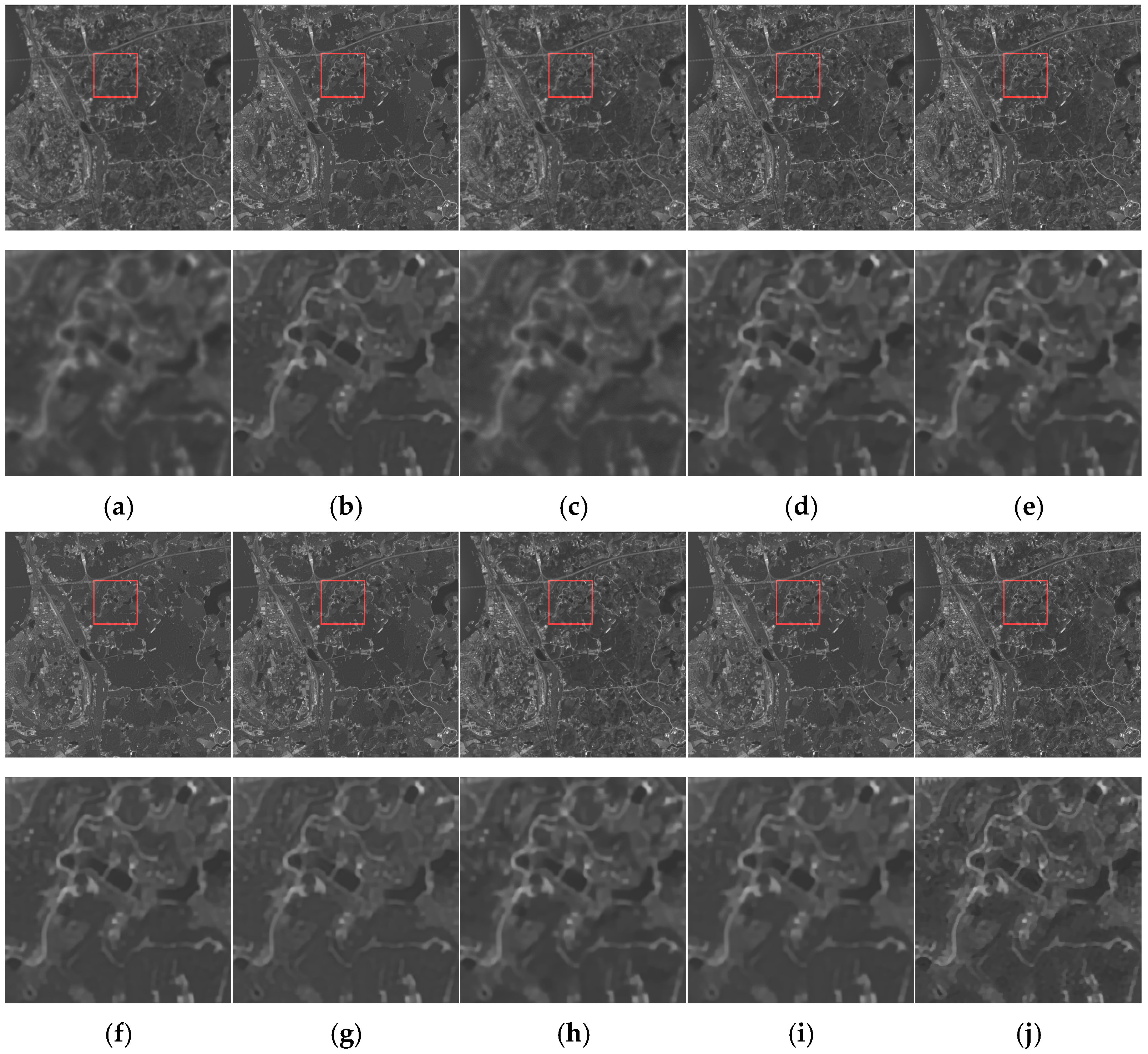
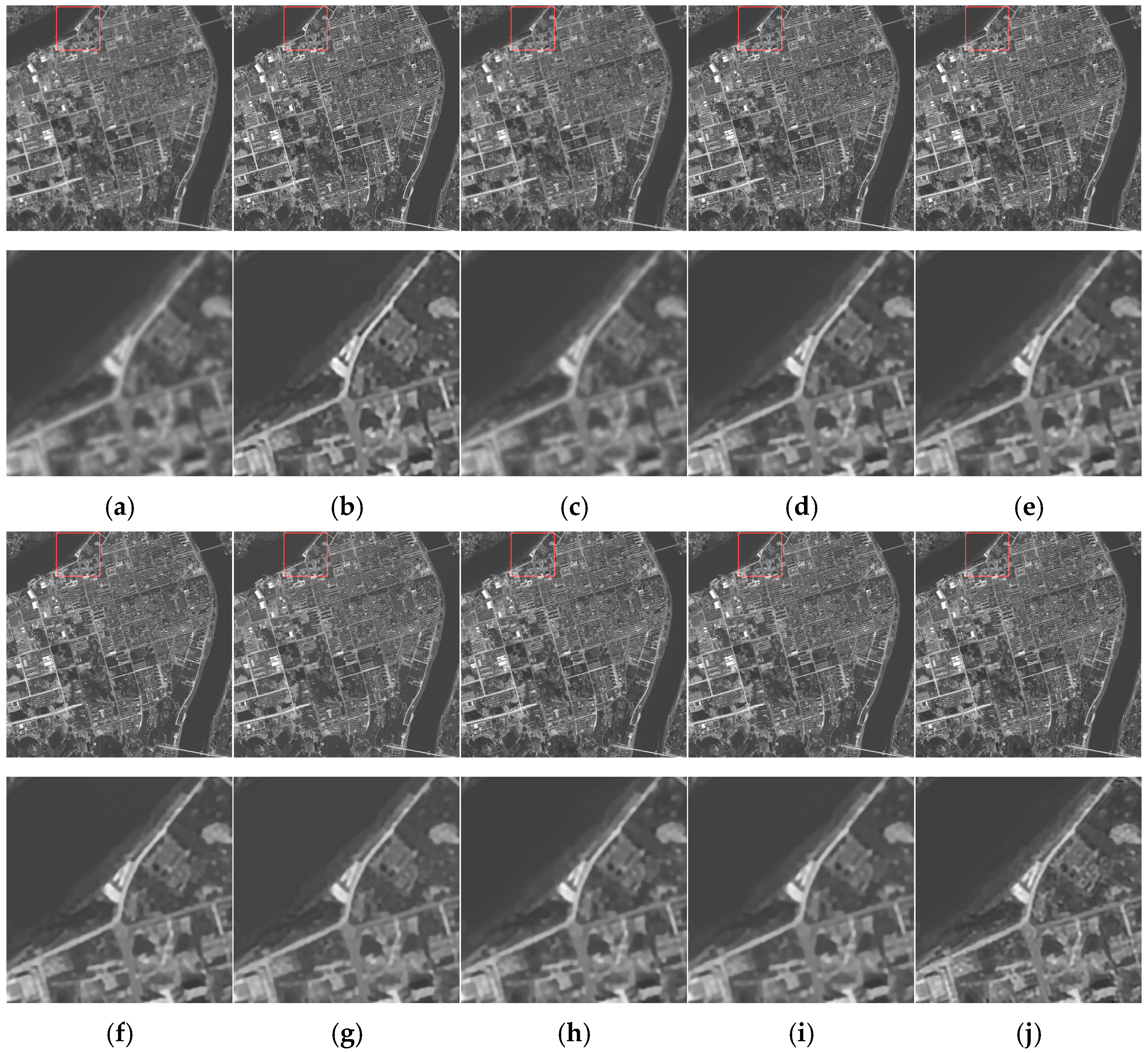
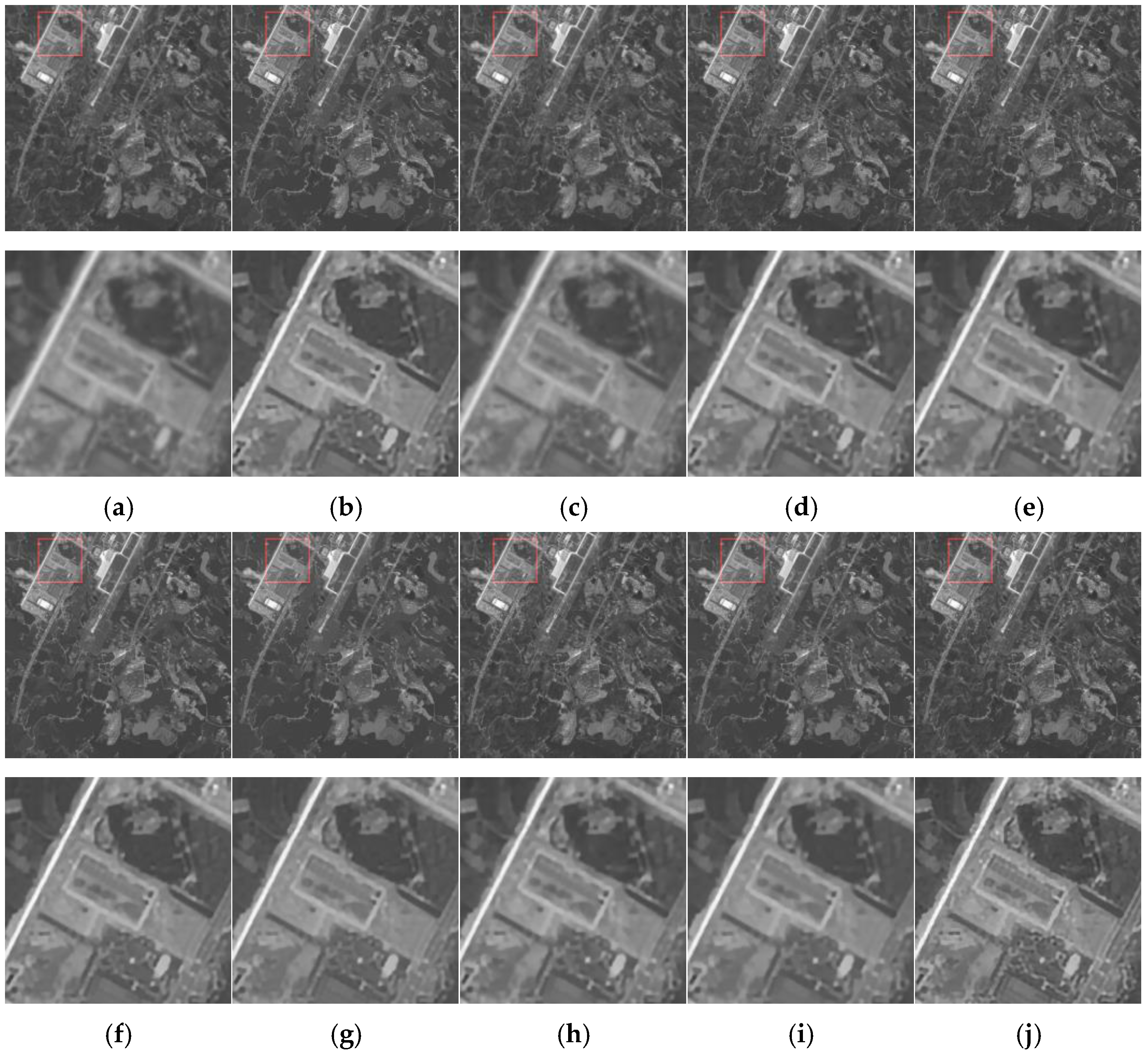
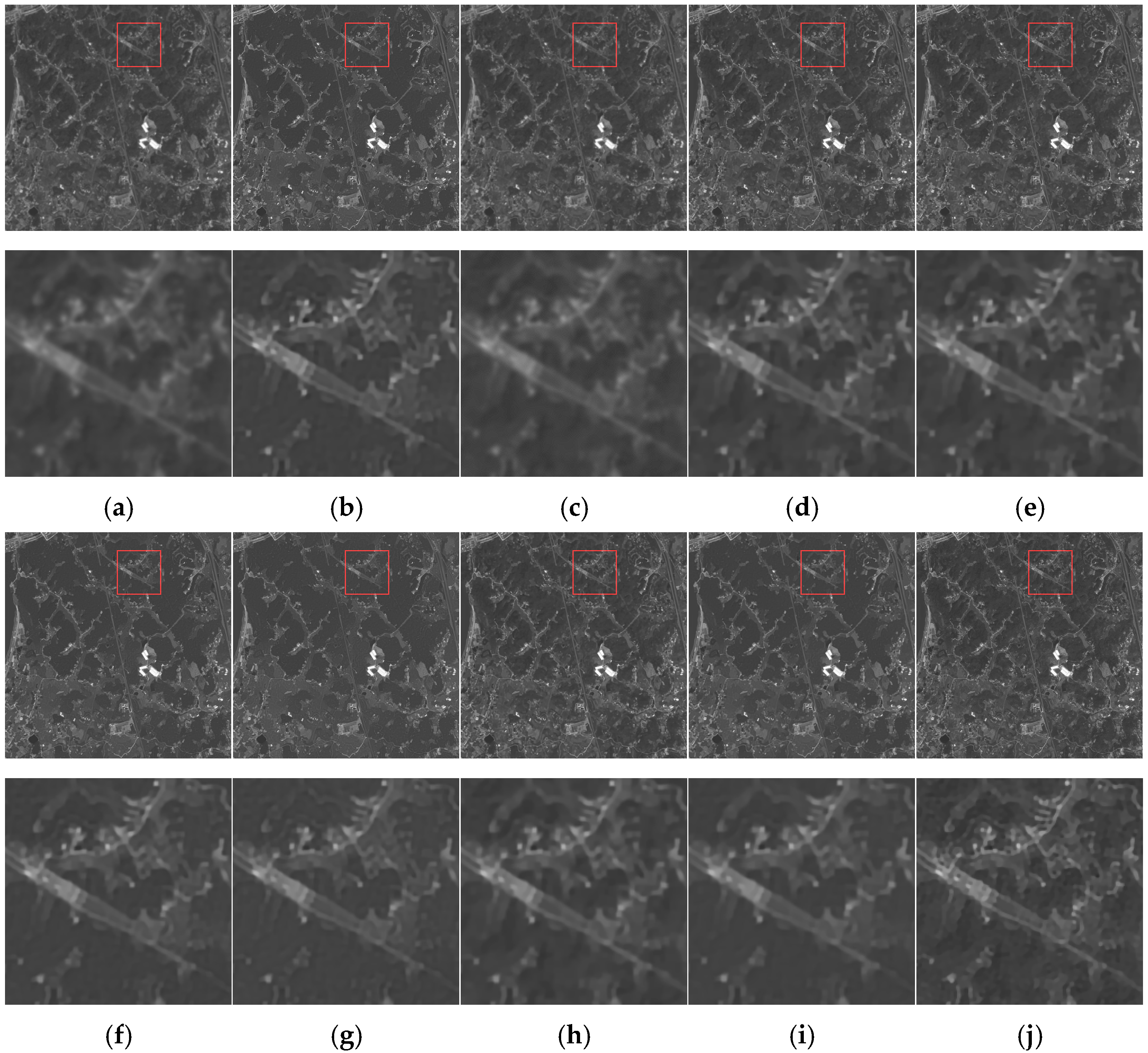
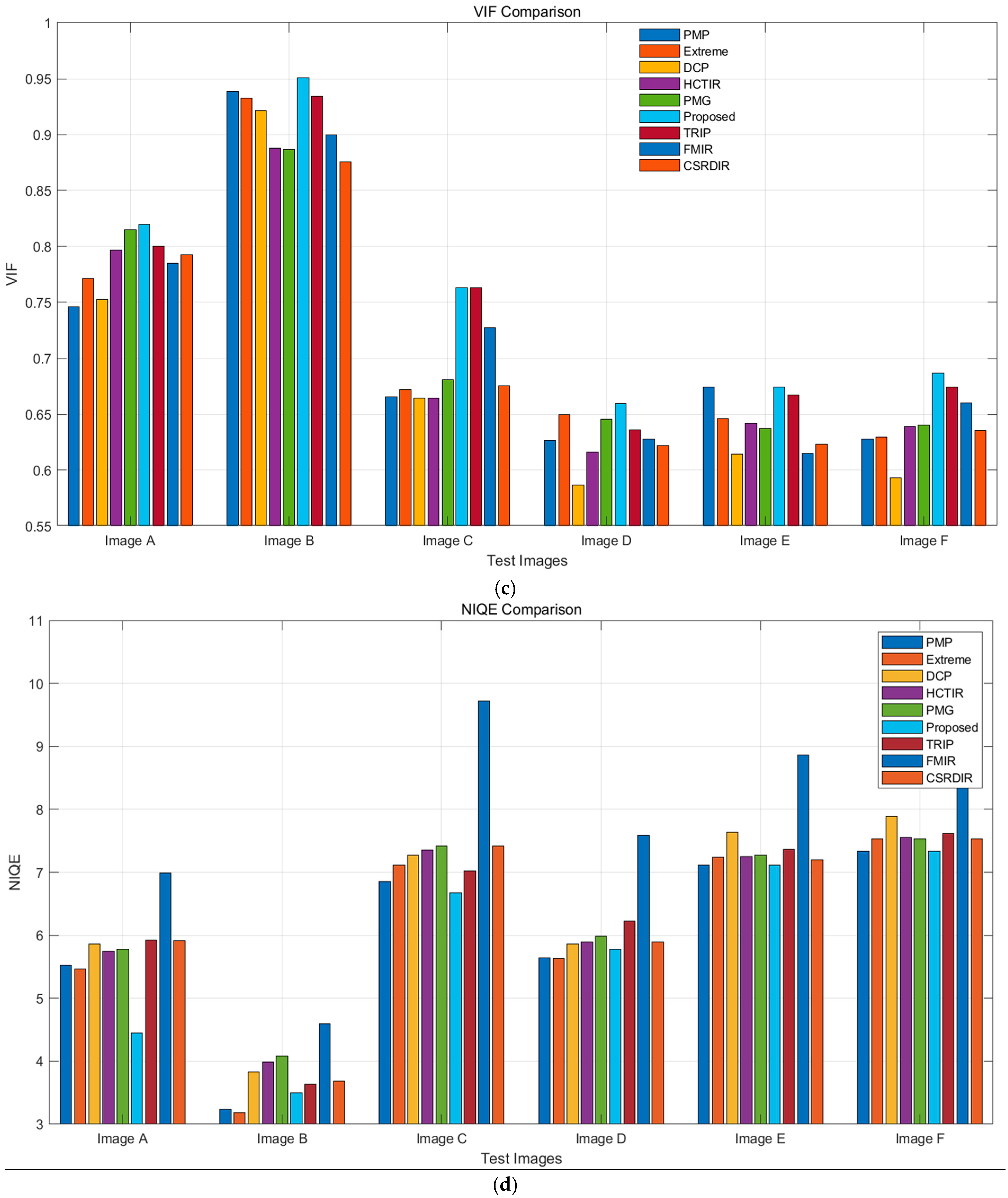
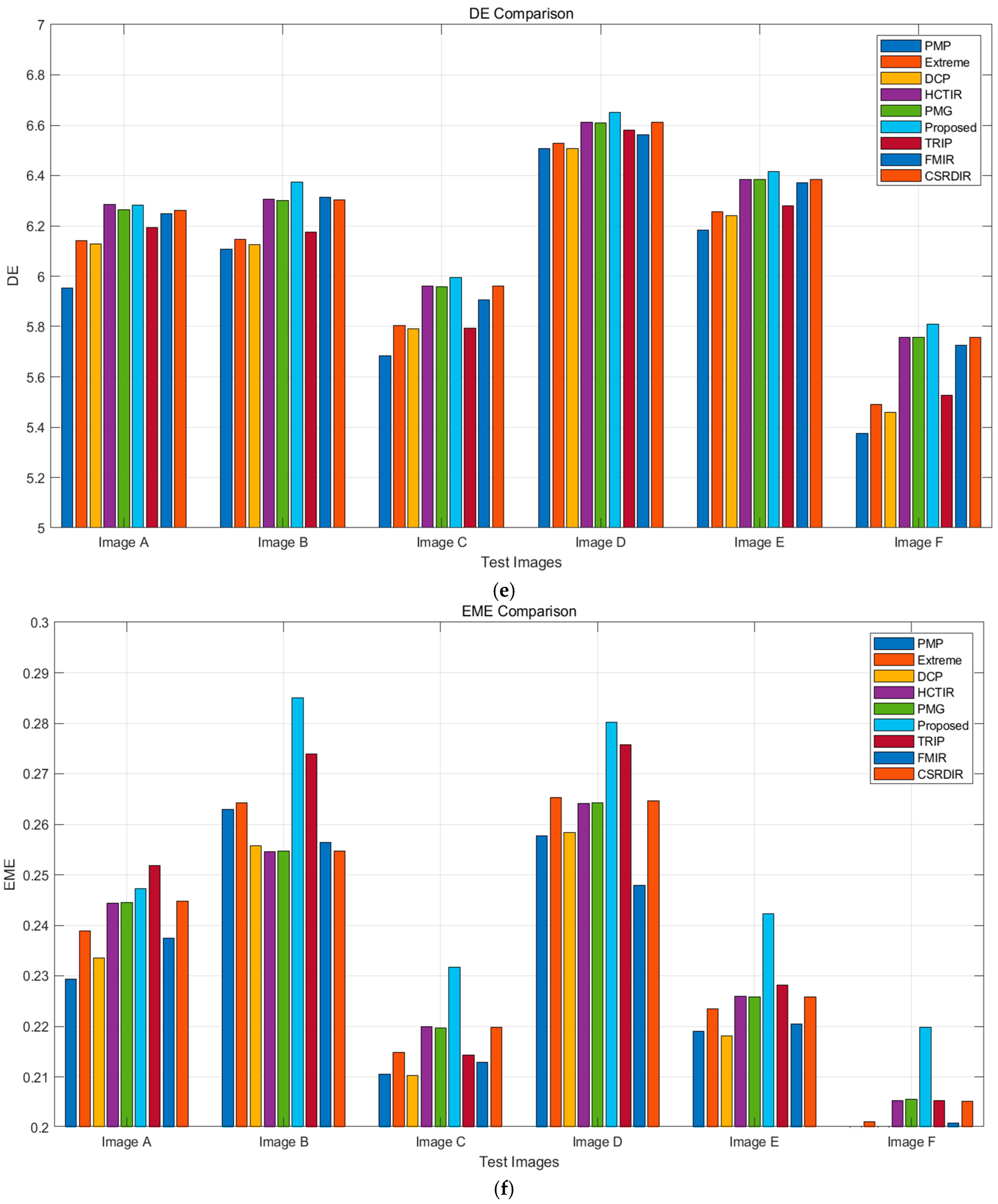
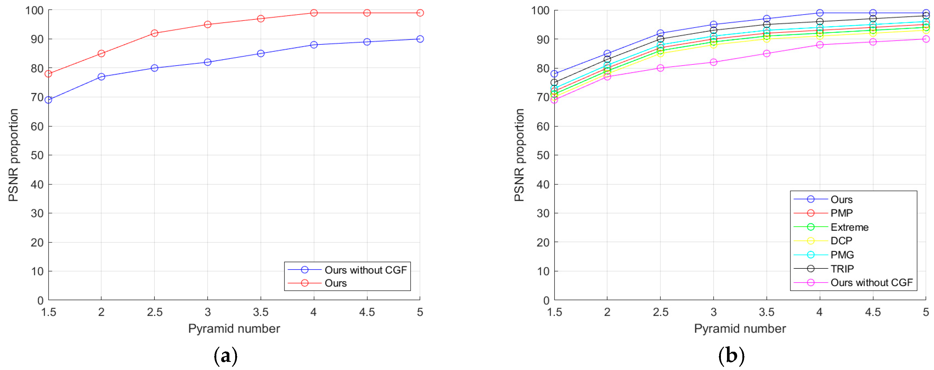
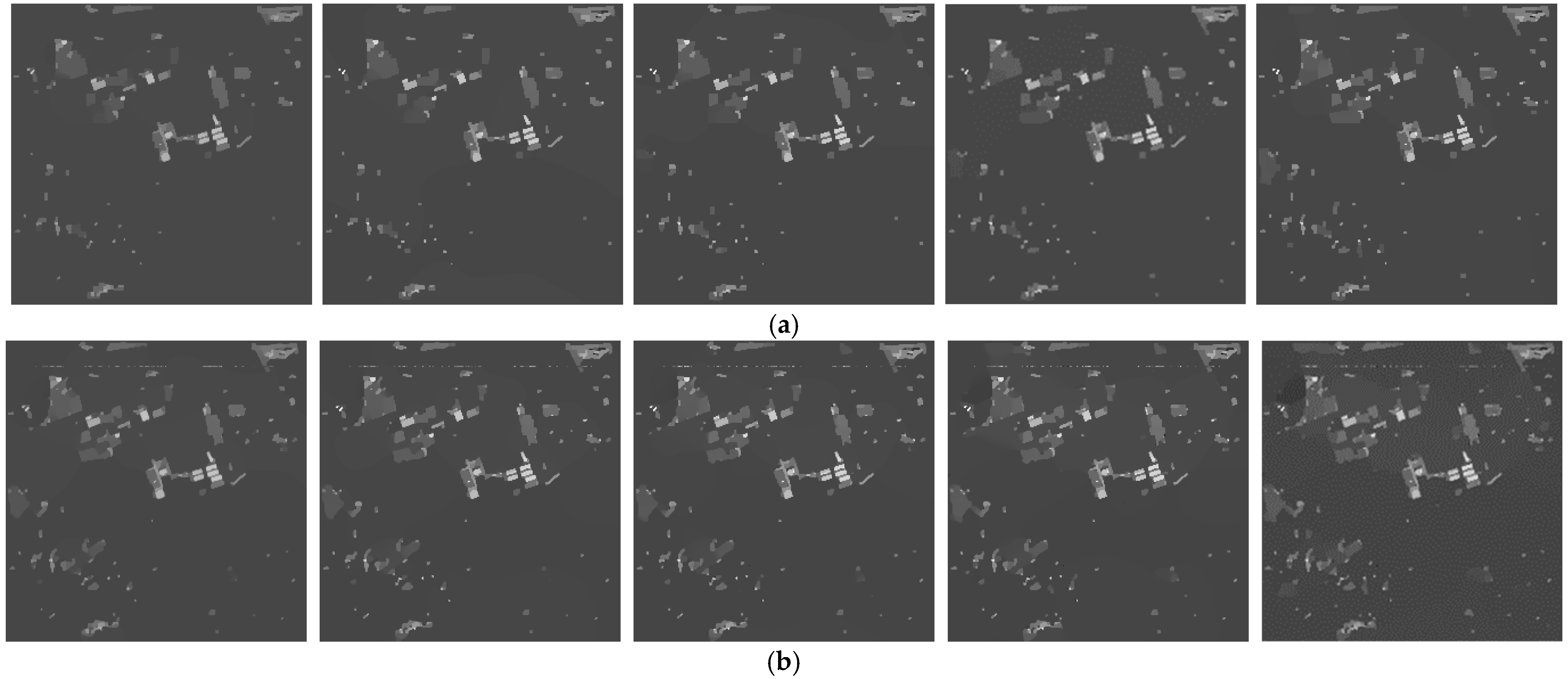
5.2. Results and Discussion

As shown in Figure 12, the proposed method outperforms other algorithms in most metrics. For PSNR, it achieves high scores (28–29 dB) on Image B and Image F. In SSIM, it performs best on Image B, nearing 0.9, and maintains a high level overall. The proposed method also excels in VIF, with a high score of around 0.95 on Image B. For NIQE, it keeps values low, indicating natural image quality with minimal distortion. In terms of DE, it performs similarly to other methods in edge preservation, and in EME, it shows strong performance, particularly on certain test images.

6. Analysis and Discussion

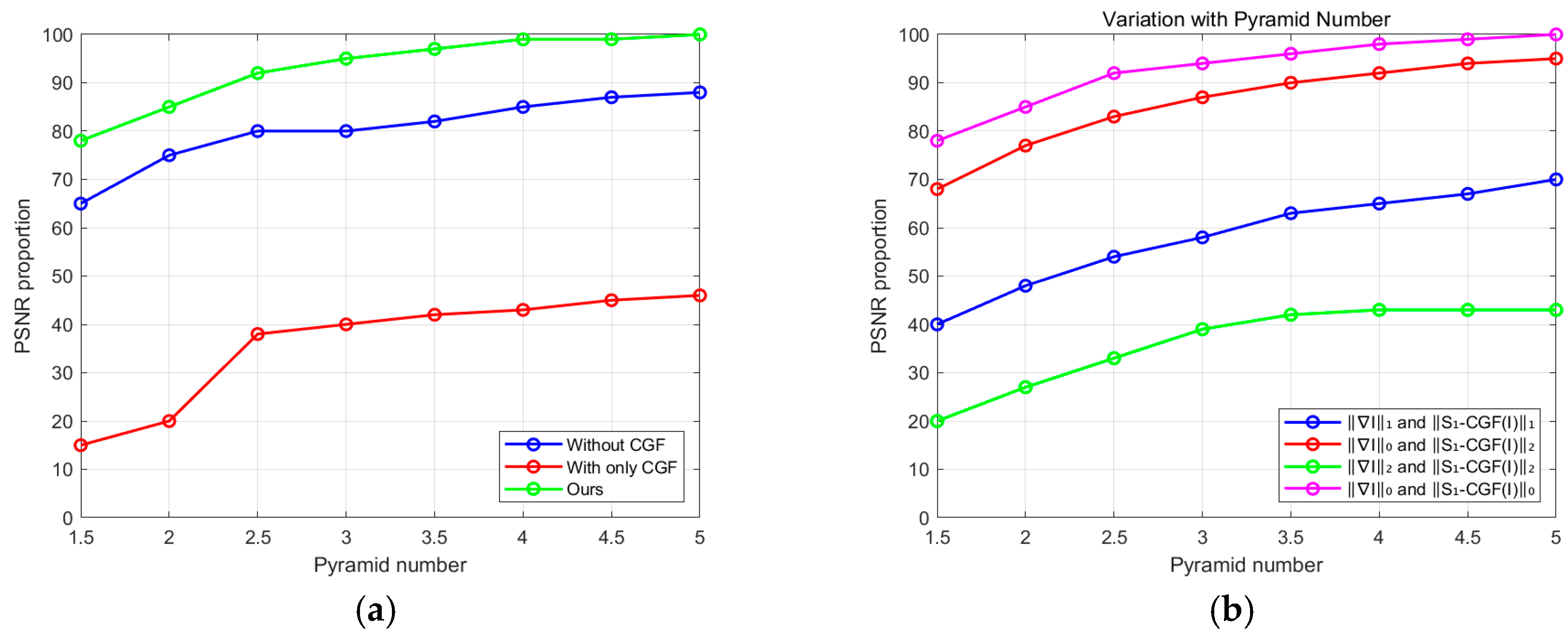
In this section, we further analyze the effectiveness of the $\mathrm{C}GF$ prior and compare it with other relevant L0 regularization methods. We investigate the impact of sparse constraints in the model, the influence of patch size in the prior term, and sensitivity to key parameters.

6.1. Effectiveness of $CGF$ Prior

As shown in Figure 13a, when conducting quantitative and qualitative evaluations on the dataset mentioned above, we compared the performance of our method with and without the utilization of $\mathrm{C}GF$ across various evaluation metrics. The results of our approach demonstrated a clear superiority over the non-$\mathrm{C}GF$-enhanced method. Our $\mathrm{C}GF$ prior significantly improves the recovery performance. Additionally, it is essential to note that our non-$\mathrm{C}GF$ approach solely incorporates the L0 regularization gradient term, similar to the method proposed in [28]. As shown in Figure 13b, our method exhibits superior performance in pyramid-level iterative computations at different scales, compared to other approaches.

By reconstructing the intermediate latent image of a specific example, we further analyzed the effectiveness of the prior term of $\mathrm{C}GF$. As illustrated in Figure 14, our method accurately estimated the kernel and yielded the best results, and the obtained intermediate latent image exhibits comprehensive details and features.

Compared to Figure 14f, the intermediate latent images obtained by other methods exhibit limited details and features, and the grayscale distribution shows a severe piecewise function pattern. In contrast, our prior term of $\mathrm{C}GF$ benefits from the prior term and detailed compensation mechanism during the iterative process. This is advantageous in generating intermediate latent images with precise edges and more prominent details, facilitating accurate kernel estimation.

It is noteworthy that solely employing the $\mathrm{C}GF$ prior for deblurring (without including the gradient smoothing term) does not achieve the desired effects. As shown in Figure 15a, methods incorporating only $\mathrm{C}GF$-related terms yield poor results on the dataset. The primary reason is that the $\mathrm{C}GF$ prior cannot directly substitute for the $‖\nabla \mathit{I}‖$ term, which constrains the edges. When using only the L0 gradient prior, the deblurring effect is also less satisfactory. However, the effective combination of the $\mathrm{C}GF$ prior and L0 gradient prior demonstrates excellent recovery performance. In summary, our $\mathrm{C}GF$ prior further facilitates the formation of sharp edges, thereby aiding in accurate kernel estimation.

6.2. Comparison with Other L0 Regularization Methods

Recently, several state-of-the-art deblurring methods [30,41,42,43,44,60] have involved L0 regularization priors. These methods primarily impose sparsity constraints on extreme channels, such as dark and bright channels [41,42] or pixel intensities [30,43]. When there are no apparent extreme channel pixels or complex pixel relationships in the image, these methods often fail to recover effectively. However, our approach is notably different. The prior term of $\mathrm{C}GF$ selectively preserves, based on the comparison between the central pixel gradient of each patch and the gradient extremes of surrounding patches. Moreover, the prior term data is determined by the gradient magnitude and directional differences, encompassing more comprehensive features rather than simply focusing on pixel intensity. As shown in Figure 14, the intermediate results generated by our proposed method based on pixel intensity during the iterative process are clearer than in other methods. In the experimental comparisons in Section 5 (results from the previous section), our method also outperforms other methods [41,42,43,60] in terms of L0 regularization.

6.3. Sparsity Constraints on the $CGF$ Prior

In our model, we employ the L0-norm to impose sparse constraints on terms related to $\mathrm{C}GF$. L2-norm and L1-norm are also commonly used for regularization of various priors. Therefore, we perform L0-, L1-, and L2-norm constraints on our $\mathrm{C}GF$-related terms (${‖{\mathit{S}}_{\mathit{I}}-\mathrm{C}GF\left(\mathit{I}\right)‖}_0$, ${‖{\mathit{S}}_{\mathit{I}}-\mathrm{C}GF\left(\mathit{I}\right)‖}_1$, ${‖{\mathit{S}}_{\mathit{I}}-\mathrm{C}GF\left(\mathit{I}\right)‖}_2$), followed by quantitative comparisons on the dataset provided using three constraint methods. As shown in Figure 15b, methods that apply L0-, L1-, or L2-norm constraints on $\mathrm{C}GF$-related terms achieve higher success rates than the non-$\mathrm{C}GF$ methods. This indicates that our $\mathrm{C}GF$ prior is an intrinsic property of the image, and its sparse constraints are more effective in recovering clear images than blurred ones. It is noteworthy that the method using L0-norm constraints on $\mathrm{C}GF$-related terms performs the best among the three compared methods. However, most other methods [44] utilize L1-norm for the regularization of the related terms.

Additionally, we employ L0-, L1-, and L2-norms to sparsely constrain gradients, combining them with our $\mathrm{C}GF$-related terms and conducting quantitative evaluations. Figure 15b shows that the methods utilizing L1 and L2 regularization on gradients fail to produce satisfactory results, with the L2-regularized gradient method exhibiting the lowest success rate and the highest error rate. This is because L1- and L2-regularization methods on gradients within the MAP framework tend to favor trivial solutions [25]. The approach that applies L0 regularization to both gradients and $\mathrm{C}GF$ priors achieves the best results; hence, we use L0-norm as the constraint for our model.

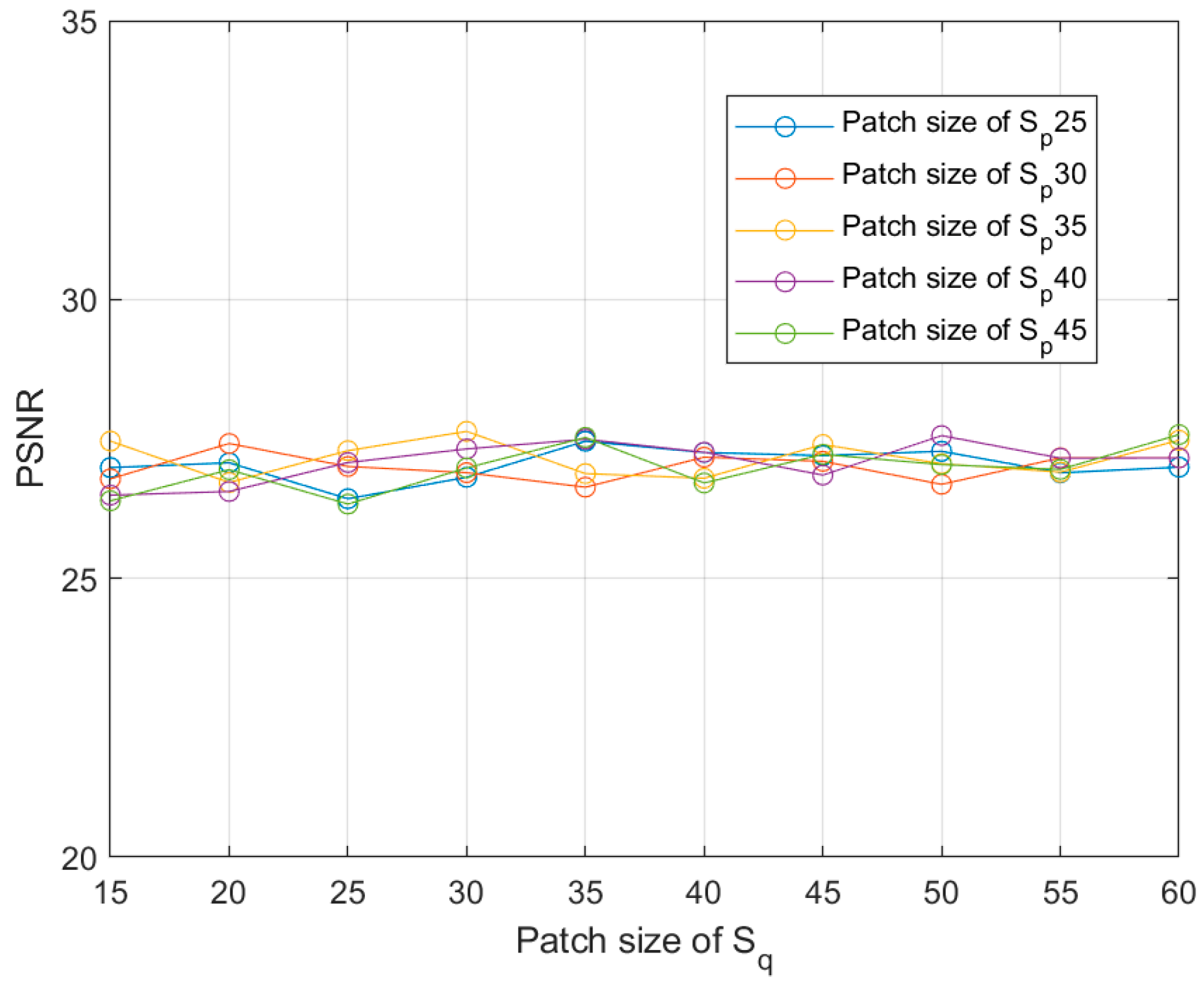
6.4. Effect of Patch Size

The choice of patch size is a crucial factor in computing the $\mathrm{C}GF$ prior. We tested different patch sizes on the dataset of “Jilin-1” in our algorithm. We computed the average PSNR for different patch sizes for quantitative comparison. As shown in Figure 16, our method exhibits insensitivity to patch size within a reasonable range. Notably, the adaptive patch method (patch size $s=0.035\cdot mean(m,n)$) achieves relatively high average PSNR, further mitigating the relative impact of patch-size settings on the recovery results. Similar adaptive patch methods can be found in [46].

6.5. Effect of Adaptive Weights for TV Model

As shown in Figure 17, Figure 18 and Figure 19, by comparing the results of non-blind deconvolution using the traditional TV model and the adaptive-weight detail-preserving deconvolution proposed in this paper with other existing methods, it is observed that the non-blind deconvolution results using our method are observed to outperform traditional TV model deconvolution in terms of grayscale contrast in flat regions and detail preservation. However, the overall deblurring effect is still inferior to the proposed method, highlighting the superior performance of our approach in solving the blur kernel. Additionally, these images demonstrate the necessity of the detail weight-preservation matrix $\mathit{A}\mathit{d}\mathit{a}$. In the region highlighted by the red circle in the figure, the image details and textures re-covered by our algorithm’s deconvolution are noticeably richer, and the comparison in Figure 17, Figure 18 and Figure 19c,d indicates that the accuracy of the blur kernel solved by the proposed method is higher.

6.6. Analysis of the Parameters

Our method primarily involves three regularization weight parameters: $\tau ,\gamma ,$ and $\beta$. We conduct a quantitative analysis of these weight parameters on the dataset from “Jilin-1” by varying one parameter at a time, while keeping the others fixed. We employ the kernel similarity metric from [71] to assess the accuracy of the estimated kernel. As depicted in Figure 20, our method demonstrates insensitivity to parameter settings within a reasonable range.

6.7. Noise Robustness Testing

To evaluate the robustness of various prior methods to noise, we degraded the images using blur kernels and then added Gaussian noise and salt-and-pepper noise of different intensities. The similarity between the estimated blur kernel and the original blur kernel used for degradation was assessed using the SSIM (Structural Similarity Index) metric, in order to test the noise robustness of the different prior terms.

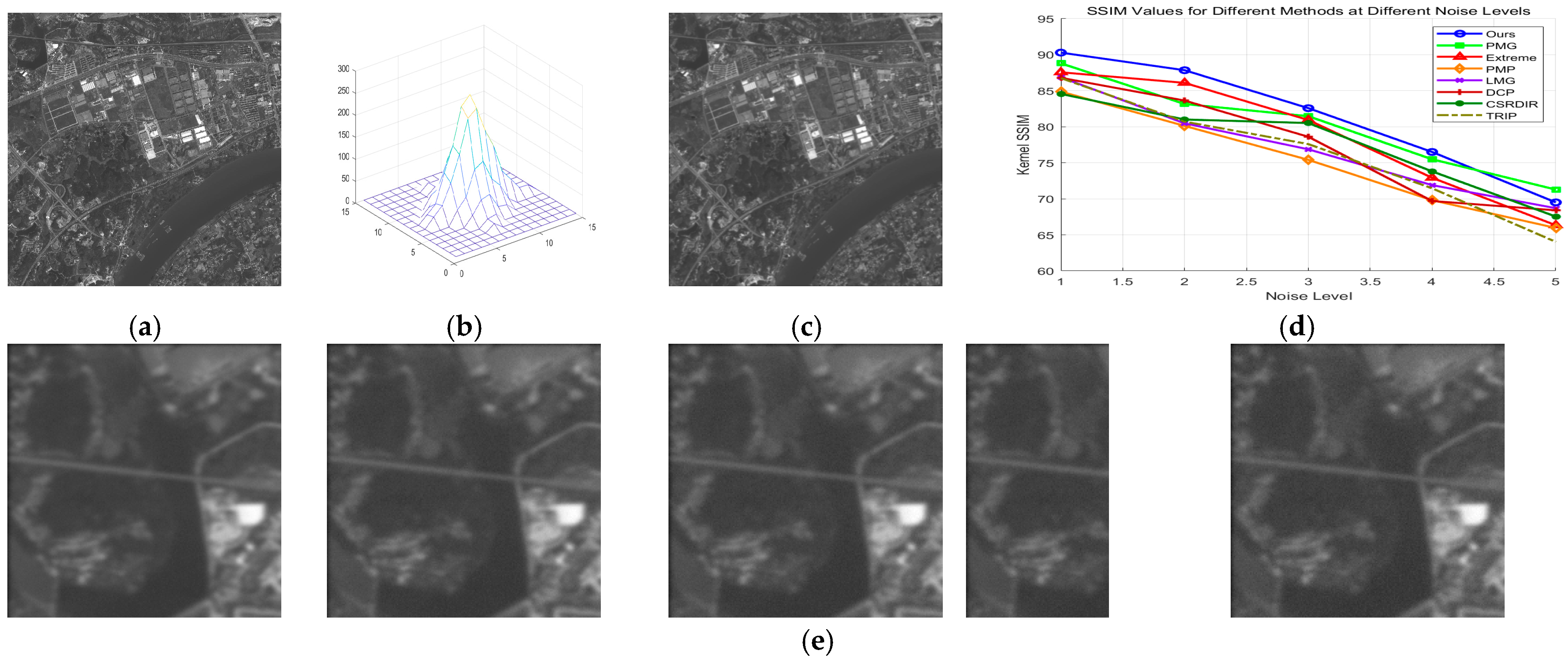
6.7.1. Gaussian Noise Robustness Testing

In Figure 21e, from left to right, the Gaussian noise density and noise amplitude gradually increase. Since our method selects strong edges as prior information, and the gradient of the true edge region in the image is still greater than the gradient difference caused by most of the noise points, the impact of Gaussian noise on the selection of edge points in our algorithm is relatively small when the noise density is low. However, as the noise amplitude increases, the accuracy of all methods decreases. If the noise density and amplitude are sufficiently large, the accuracy of the blur kernel estimation for all prior methods significantly deteriorates.

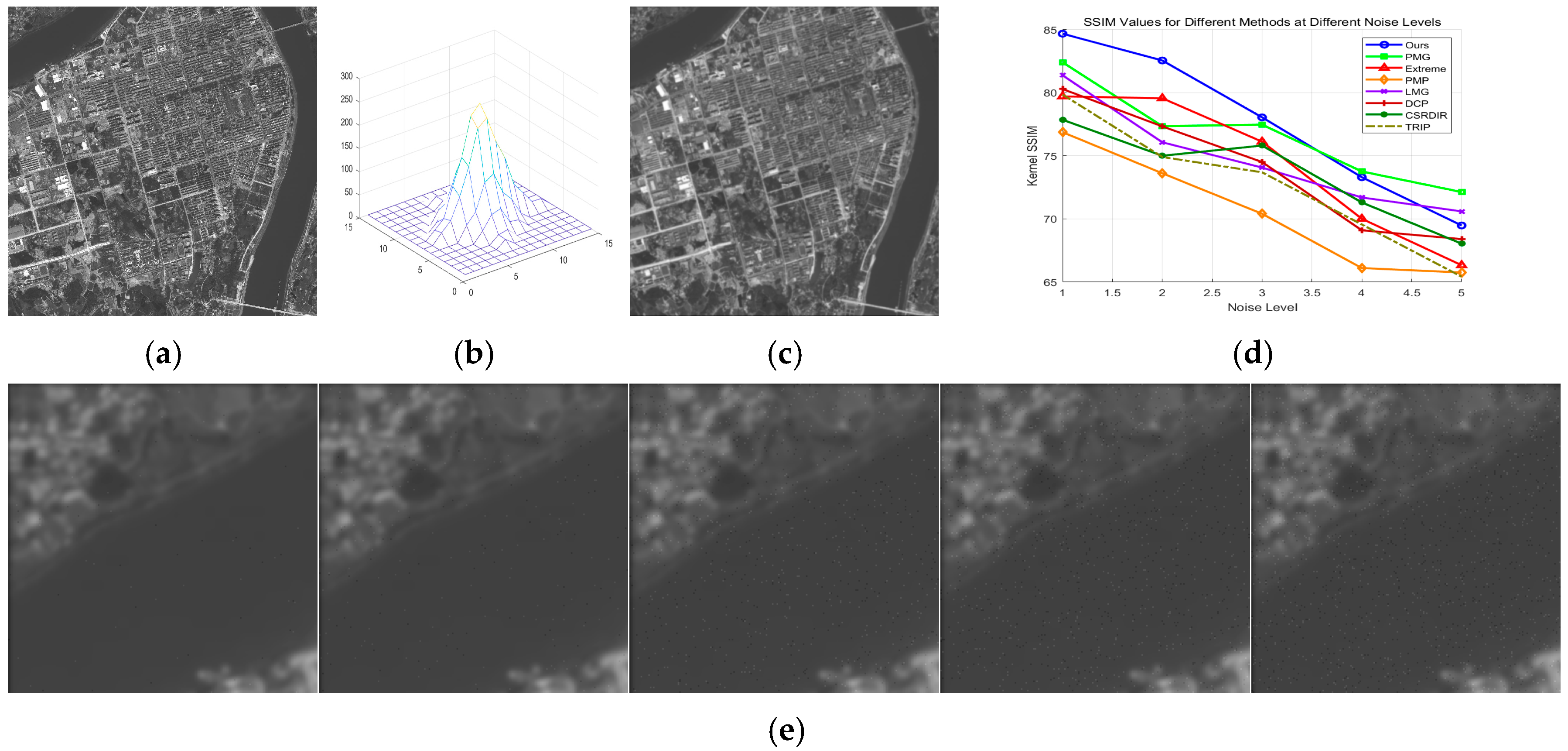
6.7.2. Salt-and-Pepper Noise Robustness Testing

In Figure 22e, from left to right, the salt-and-pepper noise density and noise amplitude gradually increase. Unlike Gaussian noise, salt-and-pepper noise typically has a higher amplitude, leading to greater differences in grayscale and gradient. As a result, the accuracy of deblurring kernels produced by various gradient-based and dark-channel improvement algorithms, including our method, is lower. When the noise density is low, our algorithm still achieves superior accuracy, but at higher noise densities, some noisy regions are mistakenly identified as edges, causing a decrease in accuracy.

7. Conclusions

To address the demand for fine processing of infrared remote-sensing images, we propose a blind infrared image deblurring algorithm based on edge gradient feature deep-sparse-diversity prior and detail preservation. Firstly, we analyze the expansion of edge regions and the variation of gradient features in remote-sensing images during the deblurring process. Based on this analysis, we introduce a prior regularization model within the MAP framework, emphasizing the preservation and compensation of edge details, leading to a refined processing approach. Experimental results demonstrate that this method achieves fine processing of remote-sensing images, accomplishing multiple objectives such as edge enhancement, texture detail preservation, and suppression of pseudo-artifacts, outperforming current methods. The proposed approach fully leverages the efficiency of remote-sensing image applications, holding high theoretical research significance and practical engineering-application value.

References

1. Torres Gil, L.K.; Valdelamar Martínez, D.; Saba, M.J.A. The widespread use of remote sensing in asbestos, vegetation, oil and gas, and geology applications. Atmosphere 2023, 14, 172. [Google Scholar] [CrossRef]
2. Li, K.; Wan, G.; Cheng, G.; Meng, L.; Han, J. Object detection in optical remote sensing images: A survey and a new benchmark. ISPRS J. Photogramm. Remote Sens. 2020, 159, 296–307. [Google Scholar] [CrossRef]
3. Li, J.; Pei, Y.; Zhao, S.; Xiao, R.; Sang, X.; Zhang, C.J.R.S. A review of remote sensing for environmental monitoring in China. Remote Sens. 2020, 12, 1130. [Google Scholar] [CrossRef]
4. Ghamisi, P.; Rasti, B.; Yokoya, N.; Wang, Q.; Hofle, B.; Bruzzone, L.; Bovolo, F.; Chi, M.; Anders, K.; Gloaguen, R.J.I.G.; et al. Multisource and multitemporal data fusion in remote sensing: A comprehensive review of the state of the art. IEEE Geosci. Remote Sens. Mag. 2019, 7, 6–39. [Google Scholar] [CrossRef]
5. Cao, Q.; Yu, G.; Qiao, Z. Application and recent progress of inland water monitoring using remote sensing techniques. Environ. Monit. Assess. 2023, 195, 125. [Google Scholar] [CrossRef]
6. Müller, R. Calibration and verification of remote sensing instruments and observations. Remote Sens. 2014, 6, 5692–5695. [Google Scholar] [CrossRef]
7. Ali, M.A.; Eltohamy, F.; Abd-Elrazek, A.; Hanafy, M.E. Assessment of micro-vibrations effect on the quality of remote sensing satellites images. Int. J. Image Data Fusion 2023, 14, 243–260. [Google Scholar] [CrossRef]
8. Serief, C.J.O.; Technology, L. Estimate of the effect of micro-vibration on the performance of the Algerian satellite (Alsat-1B) imager. Opt. Laser Technol. 2017, 96, 147–152. [Google Scholar] [CrossRef]
9. Yuan, Y.; Cai, Y.; Eyyuboğlu, H.T.; Baykal, Y.; Chen, J. Propagation factor of partially coherent flat-topped beam array in free space and turbulent atmosphere. Opt. Lasers Eng. 2012, 50, 752–759. [Google Scholar] [CrossRef]
10. Zoran, D.; Weiss, Y. From learning models of natural image patches to whole image restoration. In Proceedings of the 2011 International Conference on Computer Vision, Barcelona, Spain, 6–13 November 2011; pp. 479–486. [Google Scholar]
11. Yang, H.; Su, X.; Chen, S. Blind image deconvolution algorithm based on sparse optimization with an adaptive blur kernel estimation. Appl. Sci. 2020, 10, 2437. [Google Scholar] [CrossRef]
12. Whyte, O.; Sivic, J.; Zisserman, A. Deblurring shaken and partially saturated images. Int. J. Comput. Vis. 2014, 110, 185–201. [Google Scholar] [CrossRef]
13. Ren, M.; Delbracio, M.; Talebi, H.; Gerig, G.; Milanfar, P. Multiscale structure guided diffusion for image deblurring. In Proceedings of the IEEE/CVF International Conference on Computer Vision, Paris, France, 1–6 October 2023; pp. 10721–10733. [Google Scholar]
14. Oliveira, J.P.; Bioucas-Dias, J.M.; Figueiredo, M.A. Adaptive total variation image deblurring: A majorization–minimization approach. Signal Process. 2009, 89, 1683–1693. [Google Scholar] [CrossRef]
15. Cho, S.; Wang, J.; Lee, S. Handling outliers in non-blind image deconvolution. In Proceedings of the 2011 International Conference on Computer Vision, Barcelona, Spain, 6–13 November 2011; pp. 495–502. [Google Scholar]
16. Carbajal, G.; Vitoria, P.; Lezama, J.; Musé, P. Blind motion deblurring with pixel-wise Kernel estimation via Kernel prediction networks. IEEE Trans. Comput. Imaging 2023, 9, 928–943. [Google Scholar] [CrossRef]
17. Rasti, B.; Chang, Y.; Dalsasso, E.; Denis, L.; Ghamisi, P. Image restoration for remote sensing: Overview and toolbox. IEEE Geosci. Remote Sens. Mag. 2021, 10, 201–230. [Google Scholar] [CrossRef]
18. Quan, Y.; Wu, Z.; Ji, H.J. Gaussian kernel mixture network for single image defocus deblurring. Adv. Neural Inf. Process. Syst. 2021, 34, 20812–20824. [Google Scholar]
19. Lee, J.; Son, H.; Rim, J.; Cho, S.; Lee, S. Iterative filter adaptive network for single image defocus deblurring. In Proceedings of the IEEE/CVF Conference on Computer Vision and Pattern Recognition, Nashville, TN, USA, 20–25 June 2021; pp. 2034–2042. [Google Scholar]
20. Barman, T.; Deka, B. A Deep Learning-based Joint Image Super-resolution and Deblurring Framework. IEEE Trans. Artif. Intell. 2024, 5, 3160–3173. [Google Scholar] [CrossRef]
21. Shruthi, C.M.; Anirudh, V.R.; Rao, P.B.; Shankar, B.S.; Pandey, A. Deep Learning based Automated Image Deblurring. In Proceedings of the E3S Web of Conferences, Tamilnadu, India, 22–23 November 2023; p. 01052. [Google Scholar]
22. Wei, X.-X.; Zhang, L.; Huang, H. High-quality blind defocus deblurring of multispectral images with optics and gradient prior. Opt. Express 2020, 28, 10683–10704. [Google Scholar] [CrossRef]
23. Fergus, R.; Singh, B.; Hertzmann, A.; Roweis, S.T.; Freeman, W.T. Removing camera shake from a single photograph. In Proceedings of the SIGGRAPH06: Special Interest Group on Computer Graphics and Interactive Techniques Conference, Boston, MA, USA, 30 July–3 August 2006; pp. 787–794. [Google Scholar]
24. Shan, Q.; Jia, J.; Agarwala, A. High-quality motion deblurring from a single image. ACM Trans. Graph. 2008, 27, 1–10. [Google Scholar]
25. Levin, A.; Weiss, Y.; Durand, F.; Freeman, W.T. Understanding and evaluating blind deconvolution algorithms. In Proceedings of the 2009 IEEE Conference on Computer Vision and Pattern Recognition, Miami, FL, USA, 20–25 June 2009; pp. 1964–1971. [Google Scholar]
26. Levin, A.; Weiss, Y.; Durand, F.; Freeman, W.T. Efficient marginal likelihood optimization in blind deconvolution. In Proceedings of the CVPR 2011, Colorado Springs, CO, USA, 20–25 June 2011; pp. 2657–2664. [Google Scholar]
27. Krishnan, D.; Tay, T.; Fergus, R. Blind deconvolution using a normalized sparsity measure. In Proceedings of the CVPR 2011, Colorado Springs, CO, USA, 20–25 June 2011; pp. 233–240. [Google Scholar]
28. Xu, L.; Zheng, S.; Jia, J. Unnatural l0 sparse representation for natural image deblurring. In Proceedings of the IEEE Conference on Computer Vision and Pattern Recognition, Portland, OR, USA, 23–28 June 2013; pp. 1107–1114. [Google Scholar]
29. Pan, J.; Su, Z. Fast 0-Regularized Kernel Estimation for Robust Motion Deblurring. IEEE Signal Process. Lett. 2013, 20, 841–844. [Google Scholar]
30. Pan, J.; Hu, Z.; Su, Z.; Yang, M.-H. Deblurring text images via L0-regularized intensity and gradient prior. In Proceedings of the IEEE Conference on Computer Vision and Pattern Recognition, Columbus, OH, USA, 23–28 June 2014; pp. 2901–2908. [Google Scholar]
31. Li, J.; Lu, W. Blind image motion deblurring with L0-regularized priors. J. Vis. Commun. Image Represent. 2016, 40, 14–23. [Google Scholar] [CrossRef]
32. Xu, L.; Jia, J. Two-phase kernel estimation for robust motion deblurring. In Proceedings of the Computer Vision–ECCV 2010: 11th European Conference on Computer Vision, Heraklion, Greece, 5–11 September 2010; Proceedings, Part I 11. pp. 157–170. [Google Scholar]
33. Pan, J.; Liu, R.; Su, Z.; Gu, X. Kernel estimation from salient structure for robust motion deblurring. Signal Process. Image Commun. 2013, 28, 1156–1170. [Google Scholar] [CrossRef]
34. Cho, S.; Lee, S. Fast motion deblurring. In Proceedings of the SIGGRAPH09: Special Interest Group on Computer Graphics and Interactive Techniques Conference, New Orleans, LA, USA, 3–7 August 2009; pp. 1–8. [Google Scholar]
35. Joshi, N.; Szeliski, R.; Kriegman, D.J. PSF estimation using sharp edge prediction. In Proceedings of the 2008 IEEE Conference on Computer Vision and Pattern Recognition, Anchorage, AK, USA, 23–28 June 2008; pp. 1–8. [Google Scholar]
36. Sun, L.; Cho, S.; Wang, J.; Hays, J. Edge-based blur kernel estimation using patch priors. In Proceedings of the IEEE International Conference on Computational Photography (ICCP), Cambridge, MA, USA, 19–21 April 2013; pp. 1–8. [Google Scholar]
37. Michaeli, T.; Irani, M. Blind deblurring using internal patch recurrence. In Proceedings of the Computer Vision–ECCV 2014: 13th European Conference, Zurich, Switzerland, 6–12 September 2014; Proceedings, Part III 13. pp. 783–798. [Google Scholar]
38. Ren, W.; Cao, X.; Pan, J.; Guo, X.; Zuo, W.; Yang, M.-H. Image deblurring via enhanced low-rank prior. IEEE Trans. Image Process. 2016, 25, 3426–3437. [Google Scholar] [CrossRef] [PubMed]
39. Dong, J.; Pan, J.; Su, Z. Blur kernel estimation via salient edges and low rank prior for blind image deblurring. Signal Process. Image Commun. 2017, 58, 134–145. [Google Scholar] [CrossRef]
40. Tang, Y.; Xue, Y.; Chen, Y.; Zhou, L. Blind deblurring with sparse representation via external patch priors. Digit. Signal Process. 2018, 78, 322–331. [Google Scholar] [CrossRef]
41. Pan, J.; Sun, D.; Pfister, H.; Yang, M.-H. Blind image deblurring using dark channel prior. In Proceedings of the IEEE Conference on Computer Vision and Pattern Recognition, Las Vegas, NV, USA, 27–30 June 2016; pp. 1628–1636. [Google Scholar]
42. Yan, Y.; Ren, W.; Guo, Y.; Wang, R.; Cao, X. Image deblurring via extreme channels prior. In Proceedings of the IEEE Conference on Computer Vision and Pattern Recognition, Honolulu, HI, USA, 21–26 July 2017; pp. 4003–4011. [Google Scholar]
43. Wen, F.; Ying, R.; Liu, Y.; Liu, P.; Truong, T.-K. A simple local minimal intensity prior and an improved algorithm for blind image deblurring. IEEE Trans. Circuits Syst. Video Technol. 2020, 31, 2923–2937. [Google Scholar] [CrossRef]
44. Chen, L.; Fang, F.; Wang, T.; Zhang, G. Blind image deblurring with local maximum gradient prior. In Proceedings of the IEEE/CVF Conference on Computer Vision and Pattern Recognition, Long Beach, CA, USA, 15–20 June 2019; pp. 1742–1750. [Google Scholar]
45. Hsieh, P.-W.; Shao, P.-C. Blind image deblurring based on the sparsity of patch minimum information. Pattern Recognit. 2021, 109, 107597. [Google Scholar] [CrossRef]
46. Xu, Z.; Chen, H.; Li, Z. Fast blind deconvolution using a deeper sparse patch-wise maximum gradient prior. Signal Process. Image Commun. 2021, 90, 116050. [Google Scholar] [CrossRef]
47. Zhang, J.; Zhou, X.; Li, L.; Hu, T.; Fansheng, C. A combined stripe noise removal and deblurring recovering method for thermal infrared remote sensing images. IEEE Trans. Geosci. Remote. Sens. 2022, 60, 1–14. [Google Scholar] [CrossRef]
48. Gong, D.; Tan, M.; Zhang, Y.; Van Den Hengel, A.; Shi, Q. Self-paced kernel estimation for robust blind image deblurring. In Proceedings of the IEEE International Conference on Computer Vision, Venice, Italy, 22–29 October 2017; pp. 1661–1670. [Google Scholar]
49. Dong, J.; Pan, J.; Su, Z.; Yang, M.-H. Blind image deblurring with outlier handling. In Proceedings of the IEEE International Conference on Computer Vision, Venice, Italy, 22–29 October 2017; pp. 2478–2486. [Google Scholar]
50. Hu, Z.; Cho, S.; Wang, J.; Yang, M.-H. Deblurring low-light images with light streaks. In Proceedings of the IEEE Conference on Computer Vision and Pattern Recognition, Columbus, OH, USA, 23–28 June 2014; pp. 3382–3389. [Google Scholar]
51. Pan, J.; Hu, Z.; Su, Z.; Yang, M.-H. Deblurring face images with exemplars. In Proceedings of the Computer Vision–ECCV 2014: 13th European Conference, Zurich, Switzerland, 6–12 September 2014; Proceedings, Part VII 13. pp. 47–62. [Google Scholar]
52. Jiang, X.; Yao, H.; Zhao, S. Text image deblurring via two-tone prior. Neurocomputing 2017, 242, 1–14. [Google Scholar] [CrossRef]
53. Sun, J.; Cao, W.; Xu, Z.; Ponce, J. Learning a convolutional neural network for non-uniform motion blur removal. In Proceedings of the IEEE Conference on Computer Vision and Pattern Recognition, Boston, MA, USA, 7–12 June 2015; pp. 769–777. [Google Scholar]
54. Schuler, C.J.; Hirsch, M.; Harmeling, S.; Schölkopf, B. Learning to deblur. IEEE Trans. Pattern Anal. Mach. Intell. 2015, 38, 1439–1451. [Google Scholar] [CrossRef]
55. Chakrabarti, A. A neural approach to blind motion deblurring. In Proceedings of the Computer Vision–ECCV 2016: 14th European Conference, Amsterdam, The Netherlands, 11–14 October 2016; Proceedings, Part III 14. pp. 221–235. [Google Scholar]
56. Zhang, J.; Pan, J.; Ren, J.; Song, Y.; Bao, L.; Lau, R.W.; Yang, M.-H. Dynamic scene deblurring using spatially variant recurrent neural networks. In Proceedings of the IEEE Conference on Computer Vision and Pattern Recognition, Salt Lake City, UT, USA, 18–23 June 2018; pp. 2521–2529. [Google Scholar]
57. Nah, S.; Hyun Kim, T.; Mu Lee, K. Deep multi-scale convolutional neural network for dynamic scene deblurring. In Proceedings of the IEEE Conference on Computer Vision and Pattern Recognition, Honolulu, HI, USA, 21–26 July 2017; pp. 3883–3891. [Google Scholar]
58. Kupyn, O.; Budzan, V.; Mykhailych, M.; Mishkin, D.; Matas, J. Deblurgan: Blind motion deblurring using conditional adversarial networks. In Proceedings of the IEEE Conference on Computer Vision and Pattern Recognition, Salt Lake City, UT, USA, 18–23 June 2018; pp. 8183–8192. [Google Scholar]
59. Tao, X.; Gao, H.; Shen, X.; Wang, J.; Jia, J. Scale-recurrent network for deep image deblurring. In Proceedings of the IEEE Conference on Computer Vision and Pattern Recognition, Salt Lake City, UT, USA, 18–23 June 2018; pp. 8174–8182. [Google Scholar]
60. Li, L.; Pan, J.; Lai, W.-S.; Gao, C.; Sang, N.; Yang, M.-H. Blind image deblurring via deep discriminative priors. Int. J. Comput. Vis. 2019, 127, 1025–1043. [Google Scholar] [CrossRef]
61. Chen, M.; Quan, Y.; Xu, Y.; Ji, H. Self-supervised blind image deconvolution via deep generative ensemble learning. IEEE Trans. Circuits Syst. Video Technol. 2022, 33, 634–647. [Google Scholar] [CrossRef]
62. Quan, Y.; Yao, X.; Ji, H. Single image defocus deblurring via implicit neural inverse kernels. In Proceedings of the IEEE/CVF International Conference on Computer Vision, Paris, France, 1–6 October 2023; pp. 12600–12610. [Google Scholar]
63. Yi, S.; Li, L.; Liu, X.; Li, J.; Chen, L. HCTIRdeblur: A hybrid convolution-transformer network for single infrared image deblurring. Infrared Phys. Technol. 2023, 131, 104640. [Google Scholar] [CrossRef]
64. Young, W.H. On the multiplication of successions of Fourier constants. Proc. R. Soc. London. Ser. A Contain. Pap. A Math. Phys. Character 1912, 87, 331–339. [Google Scholar]
65. Zhou, X.; Zhang, J.; Li, M.; Su, X.; Chen, F. Thermal infrared spectrometer on-orbit defocus assessment based on blind image blur kernel estimation. Infrared Phys. Technol. 2023, 130, 104538. [Google Scholar] [CrossRef]
66. Yang, L.; Yang, J.; Yang, K. Adaptive detection for infrared small target under sea-sky complex background. Electron. Lett. 2004, 40, 1. [Google Scholar] [CrossRef]
67. Chen, B.-H.; Wu, Y.-L.; Shi, L.-F. A fast image contrast enhancement algorithm using entropy-preserving mapping prior. IEEE Trans. Circuits Syst. Video Technol. 2017, 29, 38–49. [Google Scholar] [CrossRef]
68. Mittal, A.; Soundararajan, R.; Bovik, A.C. Making a “completely blind” image quality analyzer. IEEE Signal Process. Lett. 2012, 20, 209–212. [Google Scholar] [CrossRef]
69. Zhang, H.; Wu, Y.; Zhang, L.; Zhang, Z.; Li, Y. Image deblurring using tri-segment intensity prior. Neurocomputing 2020, 398, 265–279. [Google Scholar] [CrossRef]
70. Varghese, N.; Mohan, M.R.; Rajagopalan, A.N. Fast motion-deblurring of IR images. IEEE Signal Process. Lett. 2022, 29, 459–463. [Google Scholar] [CrossRef]
71. Hu, Z.; Yang, M.H. Good regions to deblur. Computer Vision–ECCV 2012: 12th European Conference on Computer Vision, Florence, Italy, 7–13 October 2012, Proceedings, Part V.; Springer: Berlin/Heidelberg, Germany, 2012; pp. 59–72. [Google Scholar]
Figure 1. Degraded image characterization: (a) original image; (b) degraded image; (c) clear-image edge-area gradients; (d) blurred-image edge-area gradients; (f) gradient-direction difference matrix of clear images; (g) gradient-direction difference matrix of blurred images; (i) clear image E ( I ) preserves the edge region; (j) blurred image E ( I ) preserves the edge region; (k) S I C G F ( I ) of clear image; (l) S I C G F ( I ) of blurred image; (e) comparison of L1 norm of edge gradients between clear and blurred images; (h) comparison of L1 norm of gradient-direction difference matrix between clear and blurred images.
Remotesensing 16 04697 g001aRemotesensing 16 04697 g001b
Figure 2. Composition of the prior term and main flowchart of the algorithm.
Remotesensing 16 04697 g002
Figure 3. E I Mechanism for selecting edge-area gradient pixels.
Remotesensing 16 04697 g003
Figure 4. The visual differences in edge region selection of CGF(I ): (a) the grayscale differences before and after image blurring; (b) the differences in E (I) selection for edge regions before and after image blurring; (c) the (I ) differences before and after image blurring; (d) the φ(H (I )(s)) differences before and after image blurring.
Remotesensing 16 04697 g004
Figure 5. Comparison before and after intermediate latent-image detail compensation: (a) before detail compensation; (b) after detail compensation.
Remotesensing 16 04697 g005
Figure 6. Recovery results of images from image A: (a) blurred image (b) TRIP; (c) FMIR; (d) CSRDIR (e) PMG; (f) extreme; (g) PMP; (h) HCTIR; (i) DCP; (j) proposed.
Remotesensing 16 04697 g006
Figure 7. Recovery results of images from image B: (a) blurred image (b) TRIP; (c) FMIR; (d) CSRDIR (e) PMG; (f) extreme; (g) PMP; (h) HCTIR; (i) DCP; (j) proposed.
Remotesensing 16 04697 g007aRemotesensing 16 04697 g007b
Figure 8. Recovery results of images from image C: (a) blurred image (b) TRIP; (c) FMIR; (d) CSRDIR (e) PMG; (f) extreme; (g) PMP; (h) HCTIR; (i) DCP; (j) proposed.
Remotesensing 16 04697 g008
Figure 9. Recovery results of images from image D: (a) blurred image (b) TRIP; (c) FMIR; (d) CSRDIR (e) PMG; (f) extreme; (g) PMP; (h) HCTIR; (i) DCP; (j) proposed.
Remotesensing 16 04697 g009
Figure 10. Recovery results of images from image E: (a) blurred image (b) TRIP; (c) FMIR; (d) CSRDIR (e) PMG; (f) extreme; (g) PMP; (h) HCTIR; (i) DCP; (j) proposed.
Remotesensing 16 04697 g010
Figure 11. Recovery results of images from image F: (a) blurred image (b) TRIP; (c) FMIR; (d) CSRDIR (e) PMG; (f) extreme; (g) PMP; (h) HCTIR; (i) DCP; (j) proposed.
Remotesensing 16 04697 g011
Figure 12. Evaluation metrics for various methods: (a) PSNR; (b) SSIM; (c) VIF; (d) NIQE; (e) DE; (f) EME.
Remotesensing 16 04697 g012aRemotesensing 16 04697 g012bRemotesensing 16 04697 g012c
Figure 13. Quantitative evaluation of C G F prior and the other priors on the dataset: (a) contrast between our method with and without C G F ; (b) contrast of our method with other methods with the only distinction being the use of different prior terms.
Remotesensing 16 04697 g013
Figure 14. Intermediate latent-image results of our method and the other methods on the dataset: (a) intermediate latent-image results of PMG; (b) intermediate latent-image results of extreme channels; (c) intermediate latent-image results of dark channels; (d) intermediate latent-image results of PMP; (e) intermediate latent- image results of HCTIR; (f) intermediate latent-image results of ours.
Remotesensing 16 04697 g014aRemotesensing 16 04697 g014b
Figure 15. Quantitative evaluation of our method and the other methods on the dataset: (a) comparison of our method with and without C G F ; (b) comparison of our method with the other methods.
Remotesensing 16 04697 g015
Figure 16. Relationship between PSNR and the parameter patch size S p and S q . .
Remotesensing 16 04697 g016
Figure 17. Comparison of the recovery results of our method with the other methods: (a) blurred image; (b) dark-channel + traditional TV deconvolution; (c) dark-channel + edge-preservation deconvolution; (d) ours.
Remotesensing 16 04697 g017
Figure 18. Comparison of the recovery results of our method with the other methods: (a) blurred image; (b) extreme channel + traditional TV deconvolution; (c) extreme channel + edge-preservation deconvolution; (d) ours.
Remotesensing 16 04697 g018
Figure 19. Comparison of the recovery results of our method with the other methods: (a) blurred image; (b) PMP + traditional TV deconvolution; (c) PMP + edge-preservation deconvolution; (d) ours.
Remotesensing 16 04697 g019
Figure 20. Sensitivity analysis of three main parameters τ , γ , and β in our model on the dataset: (a) the parameter sensitivity of τ ; (b) the parameter sensitivity of γ ; (c) the parameter sensitivity of β .
Remotesensing 16 04697 g020
Figure 21. Gaussian noise-robustness testing results: (a) original image; (b) degenerate fuzzy kernel; (c) fuzzy kernel; (d) evaluation index of each method; (e) noisy images with different noise density levels.
Remotesensing 16 04697 g021
Figure 22. Salt-and-pepper noise-robustness testing results: (a) original image; (b) degenerate fuzzy kernel; (c) fuzzy kernel; (d) evaluation index of each method; (e) noisy images with different noise density levels.
Remotesensing 16 04697 g022
Disclaimer/Publisher’s Note: The statements, opinions and data contained in all publications are solely those of the individual author(s) and contributor(s) and not of MDPI and/or the editor(s). MDPI and/or the editor(s) disclaim responsibility for any injury to people or property resulting from any ideas, methods, instructions or products referred to in the content.