
Evaluation of Soil Moisture Retrievals from a Portable L-Band Microwave Radiometer


Abstract
1. Introduction
2. Data and Methods
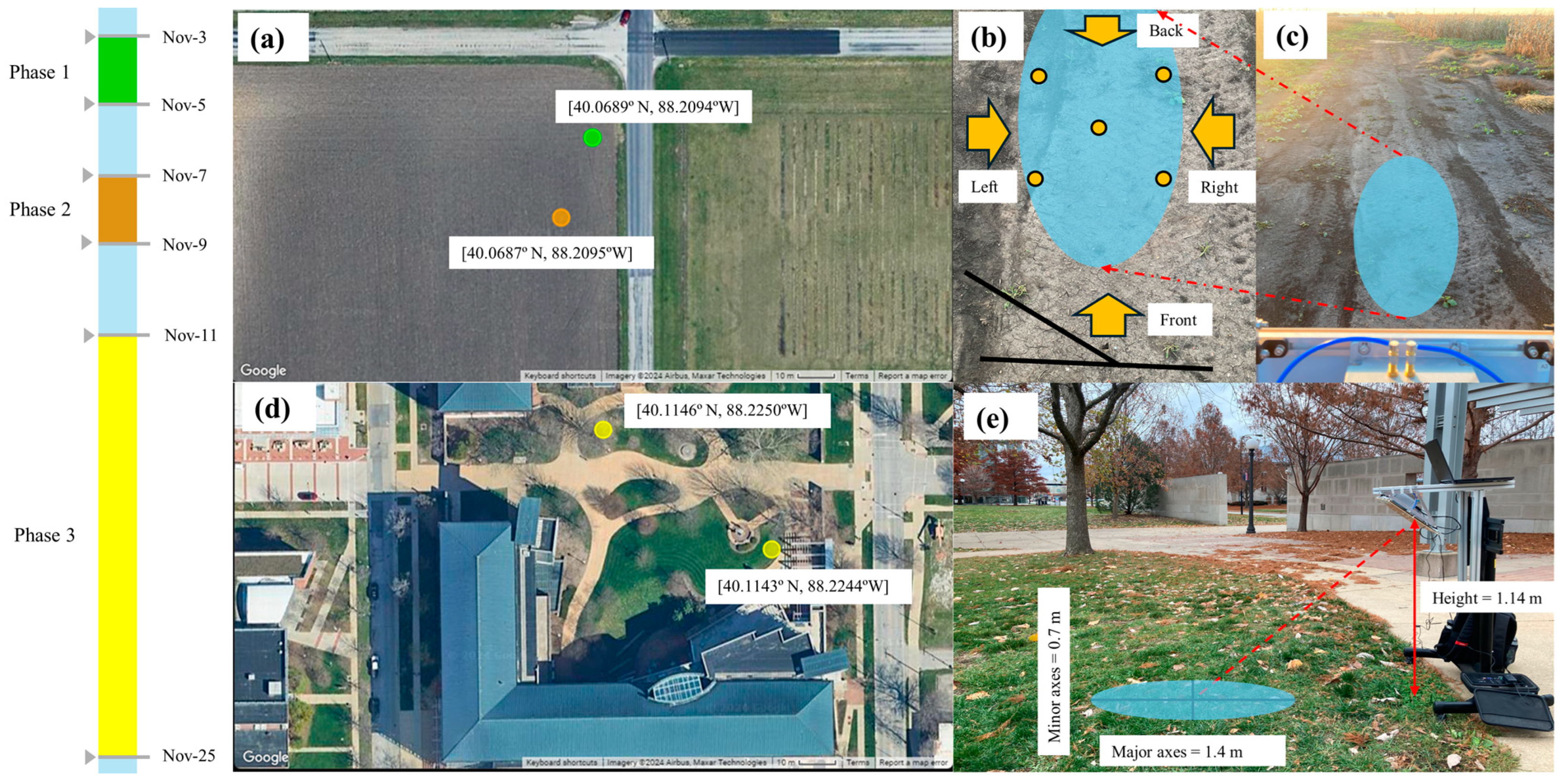
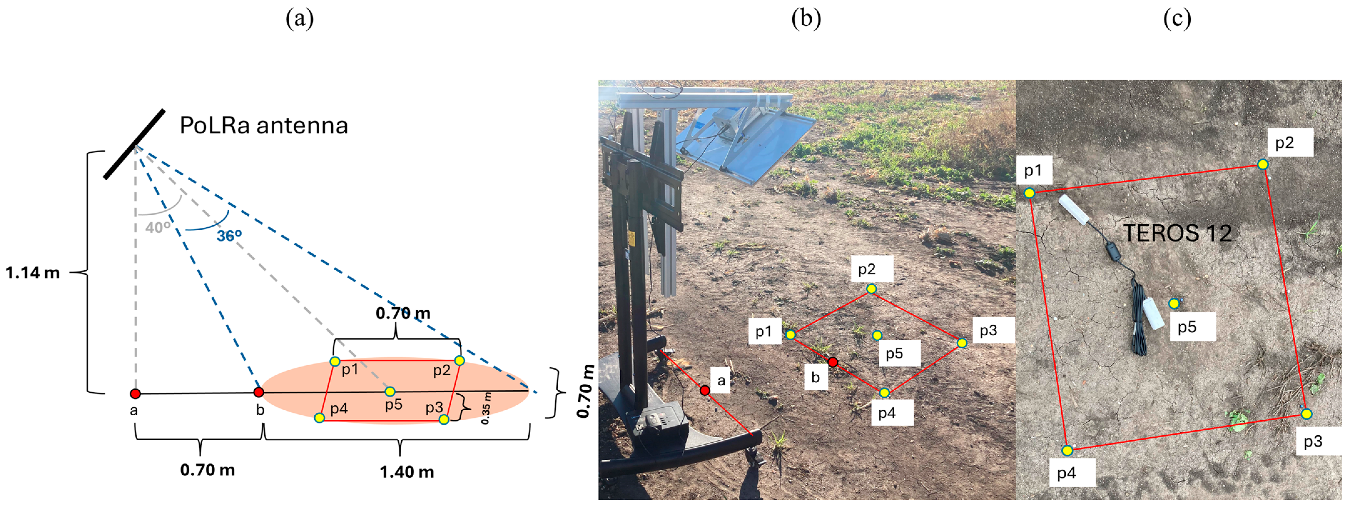
2.1. Study Sites and Experimental Timeline
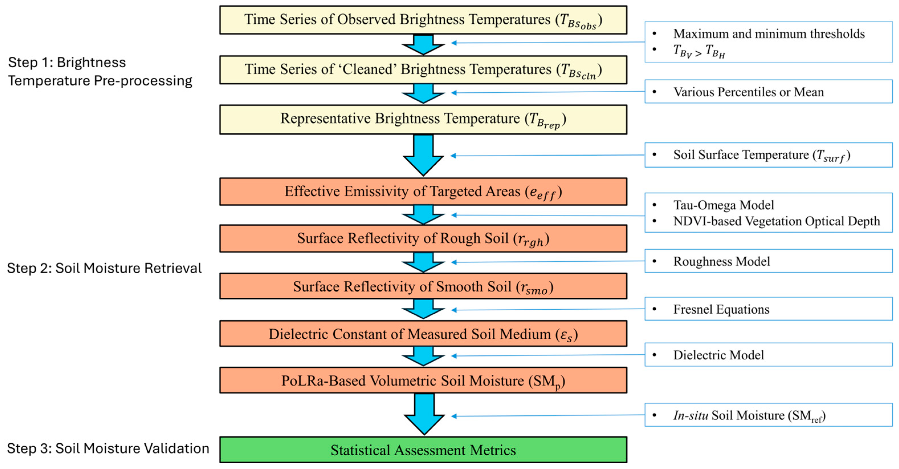
2.2. Pre-Processing of Observed Brightness Temperatures
2.3. Soil Moisture Retrieval Algorithms
2.4. Ancillary Data
2.5. Validation Scheme
3. Results
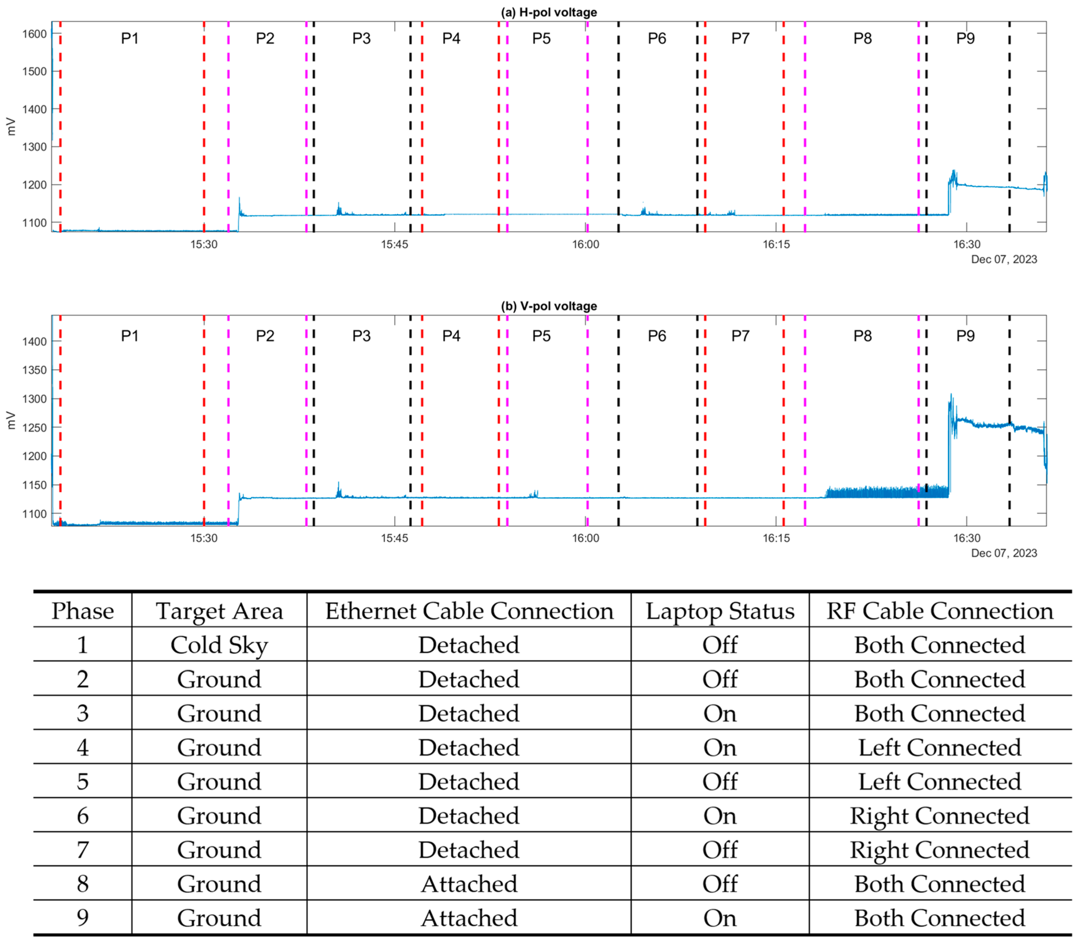
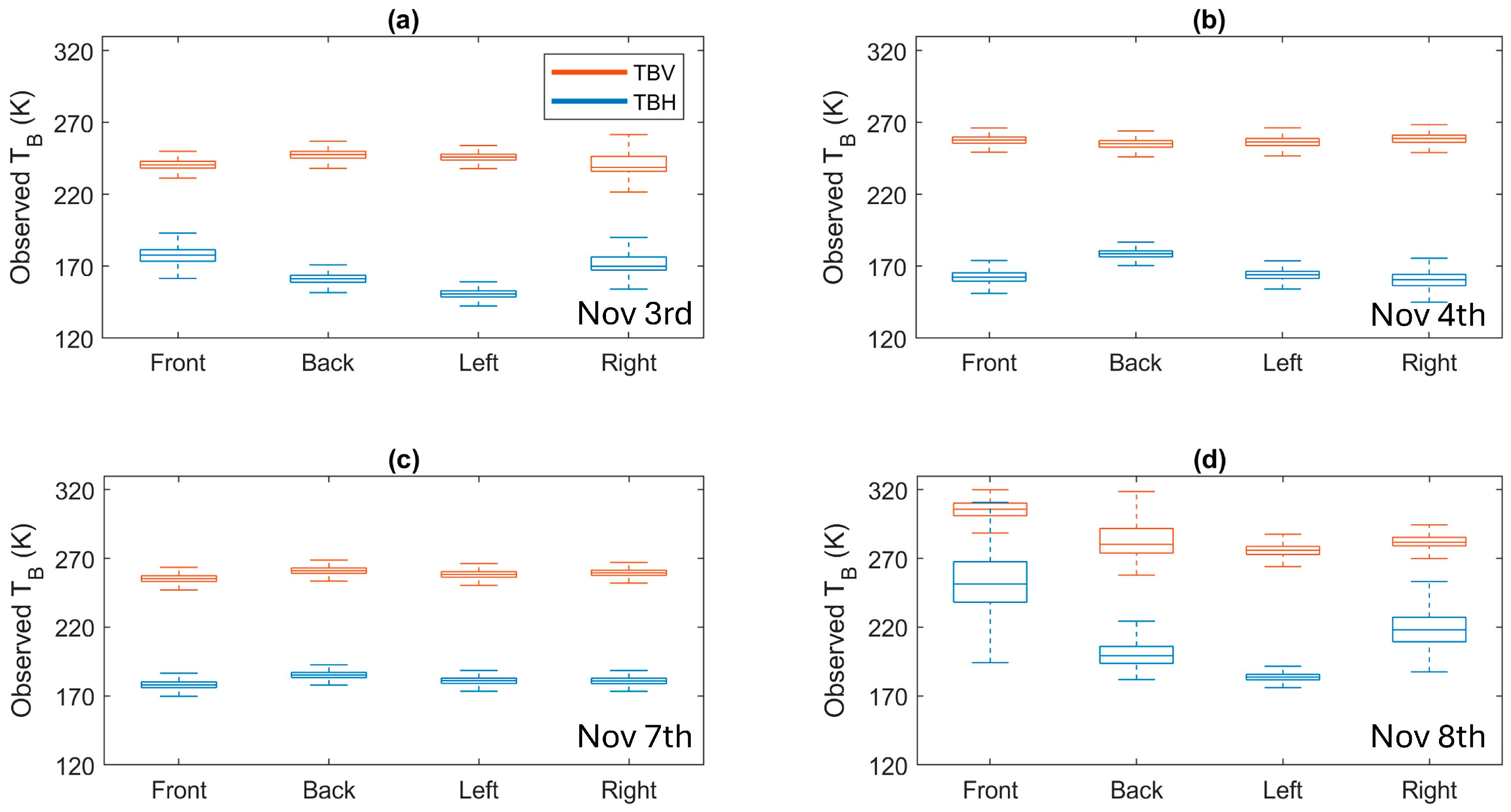
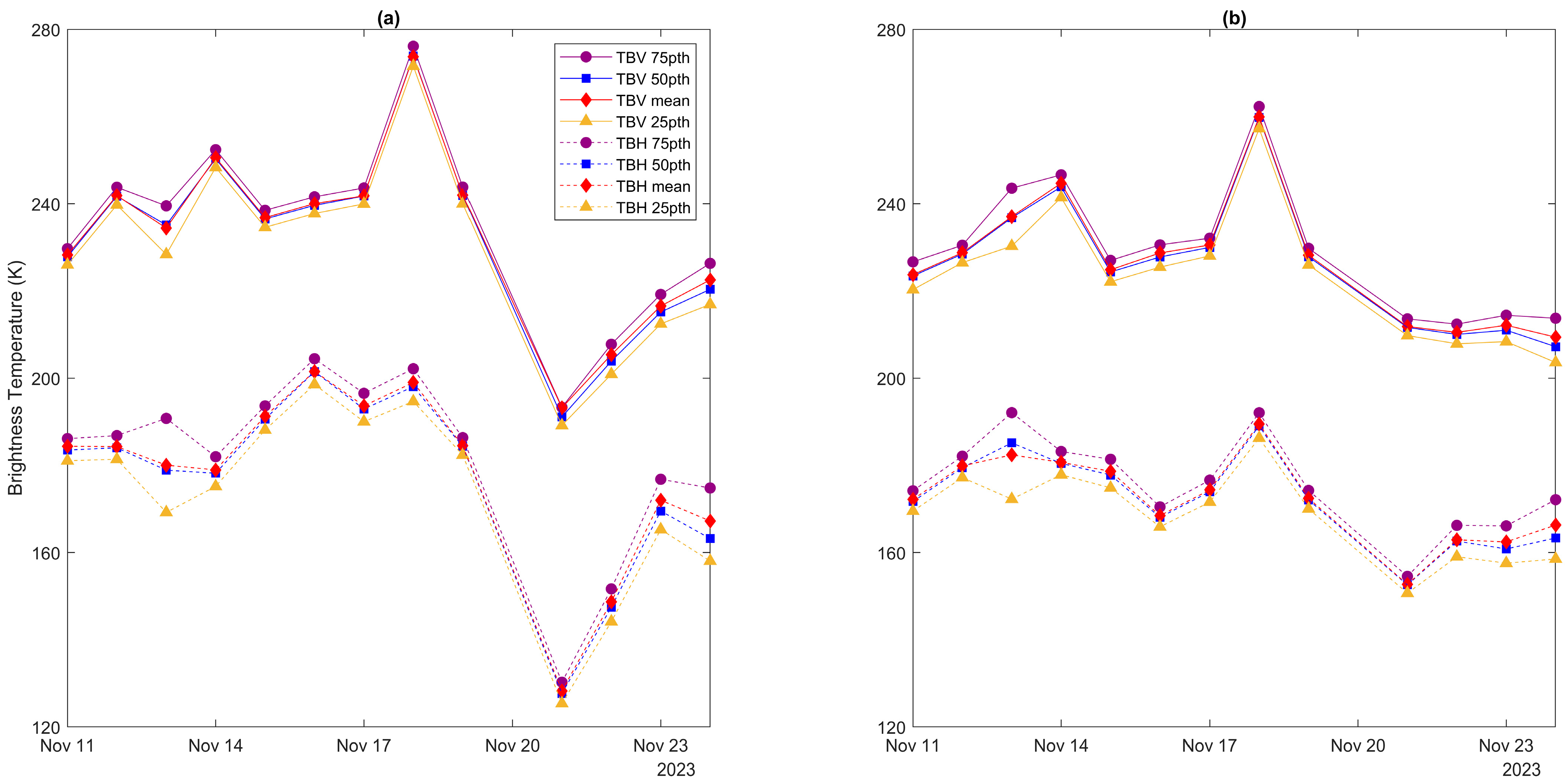
3.1. Investigation of PoLRa-Observed Brightness Temperatures
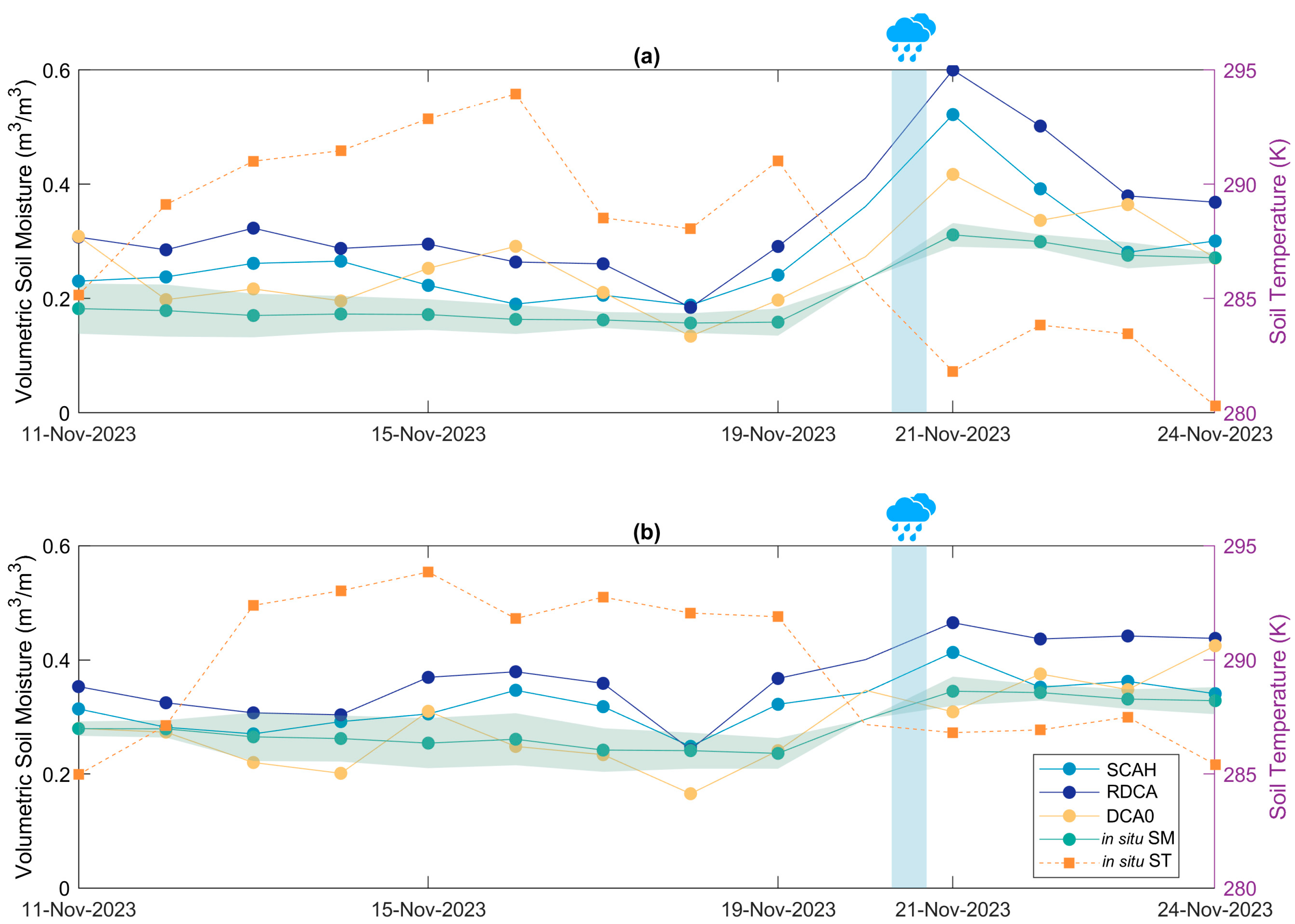
3.2. Performance of PoLRa-Derived Soil Moisture
4. Discussion
4.1. Parameter Challenges in High-Resolution Soil Moisture Retrievals
4.2. Operational and Calibration Limitations of PoLRa Measurements
4.3. Sampling Representativeness and Caveats
4.4. Other Potential Directions for PoLRa Application
5. Conclusions
- Vertically polarized brightness temperatures from PoLRa are generally more stable than their horizontally polarized counterpart.
- For any given pixel in our test, the standard deviation of brightness temperatures recorded by PoLRa from one direction is typically below 5 K.
- Under the experimental conditions adopted here, the average ubRMSE and R values for PoLRa-derived SM retrievals are generally less than 0.05 m3/m3 and greater than 0.7, respectively.
- While SMAP models and the DCA algorithm can derive SM from PoLRa observations, no single algorithm consistently outperforms the others.
Author Contributions
Funding
Data Availability Statement
Conflicts of Interest
Appendix A

| Date (Phase) | Volumetric Soil Moisture Measurements Within Pixel 1 (m3/m3) | |||||
| p1 | p2 | p3 | p4 | p5 | Mean | |
| 3 November (1) | 0.248 | 0.236 | 0.244 | 0.249 | 0.236 | 0.243 |
| 4 November (1) | 0.225 | 0.224 | 0.240 | 0.237 | 0.238 | 0.233 |
| Volumetric Soil Moisture Measurements Within Pixel 2 (m3/m3) | ||||||
| p1 | p2 | p3 | p4 | p5 | Mean | |
| 7 November (2) | 0.225 | 0.250 | 0.246 | 0.255 | 0.204 | 0.236 |
| 8 November (2) | 0.236 | 0.248 | 0.196 | 0.226 | 0.240 | 0.229 |
| Volumetric Soil Moisture Measurements Within Pixel 3 (m3/m3) (Bare Soil) | ||||||
| p1 | p2 | p3 | p4 | p5 | Mean | |
| 10 November (3) | 0.188 | 0.199 | 0.191 | 0.189 | 0.201 | 0.194 |
| 11 November (3) | 0.210 | 0.162 | 0.201 | 0.174 | 0.164 | 0.182 |
| 12 November (3) | 0.155 | 0.203 | 0.158 | 0.201 | 0.177 | 0.179 |
| 13 November (3) | 0.140 | 0.173 | 0.180 | 0.191 | 0.167 | 0.170 |
| 14 November (3) | 0.161 | 0.199 | 0.174 | 0.170 | 0.160 | 0.173 |
| 15 November (3) | 0.190 | 0.177 | 0.163 | 0.155 | 0.174 | 0.172 |
| 16 November (3) | 0.181 | 0.145 | 0.166 | 0.162 | 0.163 | 0.163 |
| 17 November (3) | 0.169 | 0.153 | 0.167 | 0.157 | 0.166 | 0.162 |
| 18 November (3) | 0.167 | 0.146 | 0.164 | 0.152 | 0.156 | 0.157 |
| 19 November (3) | 0.164 | 0.143 | 0.168 | 0.149 | 0.169 | 0.159 |
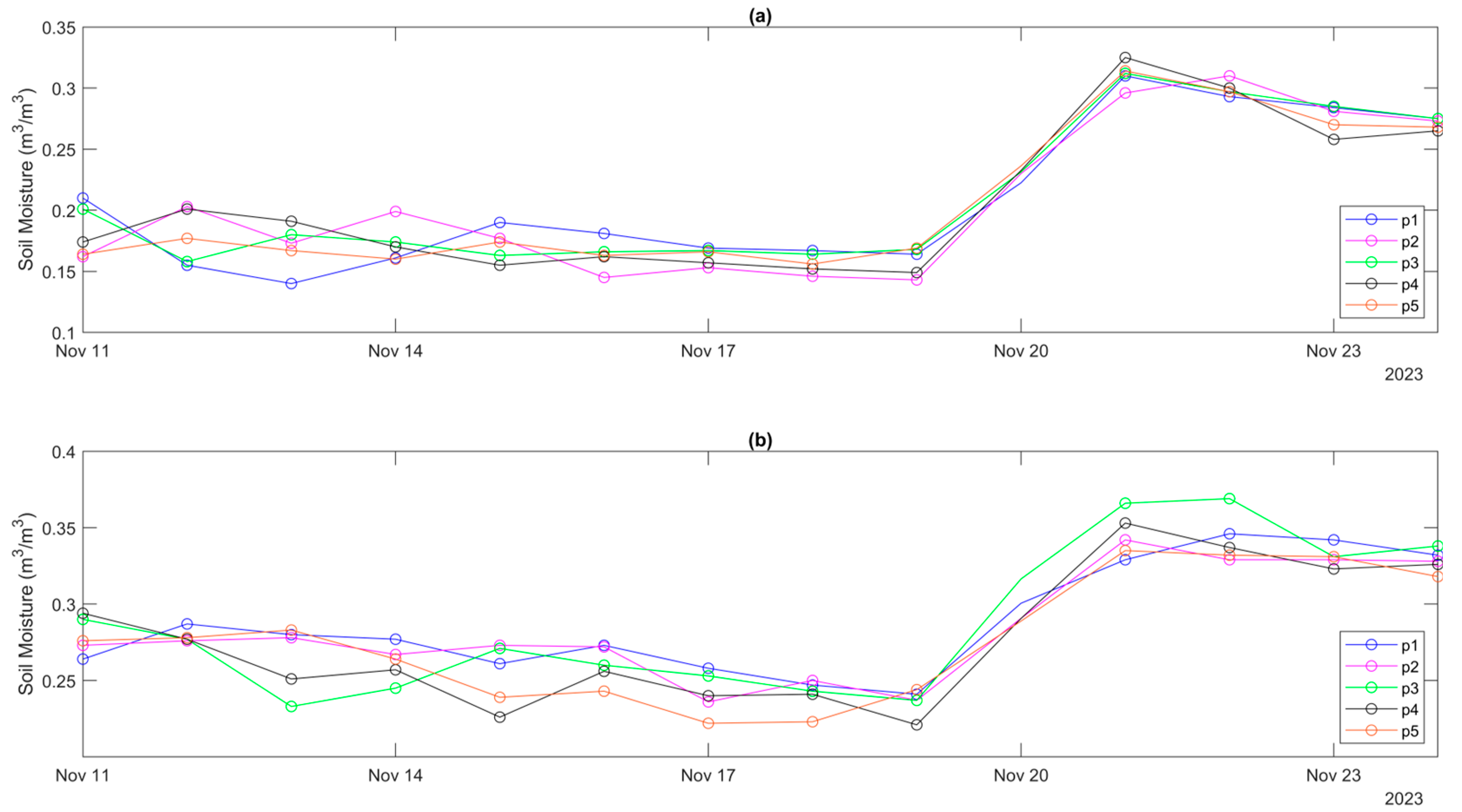
| 21 November (3) | 0.310 | 0.296 | 0.312 | 0.325 | 0.314 | 0.311 |
| 22 November (3) | 0.293 | 0.310 | 0.297 | 0.300 | 0.297 | 0.299 |
| 23 November (3) | 0.284 | 0.281 | 0.285 | 0.258 | 0.270 | 0.276 |
| 24 November (3) | 0.275 | 0.273 | 0.275 | 0.265 | 0.268 | 0.271 |
| 25 November (3) | 0.266 | 0.255 | 0.257 | 0.221 | 0.237 | 0.247 |
| Volumetric Soil Moisture Measurements Within Pixel 4 (m3/m3) (Grassland) | ||||||
| p1 | p2 | p3 | p4 | p5 | Mean | |
| 11 November (3) | 0.264 | 0.273 | 0.290 | 0.294 | 0.276 | 0.279 |
| 12 November (3) | 0.287 | 0.276 | 0.277 | 0.277 | 0.278 | 0.279 |
| 13 November (3) | 0.280 | 0.278 | 0.233 | 0.251 | 0.283 | 0.265 |
| 14 November (3) | 0.277 | 0.267 | 0.245 | 0.257 | 0.264 | 0.262 |
| 15 November (3) | 0.261 | 0.273 | 0.271 | 0.226 | 0.239 | 0.254 |
| 16 November (3) | 0.273 | 0.272 | 0.260 | 0.256 | 0.243 | 0.261 |
| 17 November (3) | 0.258 | 0.236 | 0.253 | 0.240 | 0.222 | 0.242 |
| 18 November (3) | 0.247 | 0.250 | 0.243 | 0.241 | 0.223 | 0.241 |
| 19 November (3) | 0.241 | 0.237 | 0.237 | 0.221 | 0.244 | 0.236 |
| 21 November (3) | 0.329 | 0.342 | 0.366 | 0.353 | 0.335 | 0.345 |
| 22 November (3) | 0.346 | 0.329 | 0.369 | 0.337 | 0.332 | 0.343 |
| 23 November (3) | 0.342 | 0.329 | 0.331 | 0.323 | 0.331 | 0.331 |
| 24 November (3) | 0.332 | 0.328 | 0.338 | 0.326 | 0.318 | 0.328 |
References
- Koster, R.D.; Dirmeyer, P.A.; Guo, Z.; Bonan, G.; Chan, E.; Cox, P.; Gordon, C.T.; Kanae, S.; Kowalczyk, E.; Lawrence, D.; et al. Regions of strong coupling between soil moisture and precipitation. Science 2004, 305, 1138–1140. [Google Scholar] [CrossRef] [PubMed]
- Seneviratne, S.I.; Corti, T.; Davin, E.L.; Hirschi, M.; Jaeger, E.B.; Lehner, I.; Orlowsky, B.; Teuling, A.J. Investigating soil moisture–climate interactions in a changing climate: A review. Earth-Sci. Rev. 2010, 99, 125–161. [Google Scholar] [CrossRef]
- Ge, Y.; Thomasson, J.A.; Sui, R. Remote sensing of soil properties in precision agriculture: A review. Front. Earth Sci. 2011, 5, 229–238. [Google Scholar] [CrossRef]
- Petropoulos, G. Remote Sensing of Energy Fluxes and Soil Moisture Content; CRC press: Boca Raton, FL, USA, 2013. [Google Scholar]
- Miralles, D.G.; Teuling, A.J.; Van Heerwaarden, C.C.; Vilà-Guerau de Arellano, J. Mega-heatwave temperatures due to combined soil desiccation and atmospheric heat accumulation. Nat. Geosci. 2014, 7, 345–349. [Google Scholar] [CrossRef]
- Feldman, A.F.; Short Gianotti, D.J.; Trigo, I.F.; Salvucci, G.D.; Entekhabi, D. Satellite-based assessment of land surface energy partitioning–soil moisture relationships and effects of confounding variables. Water Resour. Res. 2019, 55, 10657–10677. [Google Scholar] [CrossRef]
- Dai, A.; Trenberth, K.E.; Qian, T. A global dataset of Palmer Drought Severity Index for 1870–2002: Relationship with soil moisture and effects of surface warming. J. Hydrometeorol. 2004, 5, 1117–1130. [Google Scholar] [CrossRef]
- Feldman, A.F.; Short Gianotti, D.J.; Dong, J.; Akbar, R.; Crow, W.T.; McColl, K.A.; Konings, A.G.; Nippert, J.B.; Tumber-Dávila, S.J.; Holbrook, N.M.; et al. Remotely sensed soil moisture can capture dynamics relevant to plant water uptake. Water Resour. Res. 2023, 59, e2022WR033814. [Google Scholar] [CrossRef]
- Schmugge, T.; Choudhury, B. A comparison of radiative transfer models for predicting the microwave emission from soils. Radio Sci. 1981, 16, 927–938. [Google Scholar] [CrossRef]
- Schmugge, T. Remote sensing of surface soil moisture. J. Appl. Meteorol. 1978, 17, 1549–1557. [Google Scholar] [CrossRef]
- Ulaby, F.T.; Bradley, G.A.; Dobson, M.C. Microwave backscatter dependence on surface roughness, soil moisture, and soil texture: Part II-vegetation-covered soil. IEEE Trans. Geosci. Electron. 1979, 17, 33–40. [Google Scholar] [CrossRef]
- Ulaby, F.T.; Moore, R.K.; Fung, A.K. Microwave Remote Sensing: Active and Passive. Volume 3-From Theory to Applications; Artech House: Norwood, MA, USA, 1986. [Google Scholar]
- Njoku, E.G.; Entekhabi, D. Passive microwave remote sensing of soil moisture. J. Hydrol. 1996, 184, 101–129. [Google Scholar] [CrossRef]
- Kerr, Y.H.; Waldteufel, P.; Wigneron, J.-P.; Martinuzzi, J.; Font, J.; Berger, M. Soil moisture retrieval from space: The Soil Moisture and Ocean Salinity (SMOS) mission. IEEE Trans. Geosci. Remote Sens. 2001, 39, 1729–1735. [Google Scholar] [CrossRef]
- Entekhabi, D.; Njoku, E.G.; O’Neill, P.E.; Kellogg, K.H.; Crow, W.T.; Edelstein, W.N.; Entin, J.K.; Goodman, S.D.; Jackson, T.J.; Johnson, J.; et al. The soil moisture active passive (SMAP) mission. Proc. IEEE 2010, 98, 704–716. [Google Scholar] [CrossRef]
- Njoku, E.G.; Jackson, T.J.; Lakshmi, V.; Chan, T.K.; Nghiem, S.V. Soil moisture retrieval from AMSR-E. IEEE Trans. Geosci. Remote Sens. 2003, 41, 215–229. [Google Scholar] [CrossRef]
- Wagner, W.; Hahn, S.; Kidd, R.; Melzer, T.; Bartalis, Z.; Hasenauer, S.; Figa-Saldaña, J.; De Rosnay, P.; Jann, A.; Schneider, S.; et al. The ASCAT soil moisture product: A review of its specifications, validation results, and emerging applications. Meteorol. Z. 2013, 22, 5–33. [Google Scholar] [CrossRef]
- Imaoka, K.; Kachi, M.; Kasahara, M.; Ito, N.; Nakagawa, K.; Oki, T. Instrument performance and calibration of AMSR-E and AMSR2. Int. Arch. Photogramm. Remote Sens. Spat. Inf. Sci. 2010, 38, 13–18. [Google Scholar]
- Torres, R.; Snoeij, P.; Geudtner, D.; Bibby, D.; Davidson, M.; Attema, E.; Potin, P.; Rommen, B.; Floury, N.; Brown, M.; et al. GMES Sentinel-1 mission. Remote Sens. Environ. 2012, 120, 9–24. [Google Scholar] [CrossRef]
- Zhang, R.; Kim, S.; Sharma, A. A comprehensive validation of the SMAP Enhanced Level-3 Soil Moisture product using ground measurements over varied climates and landscapes. Remote Sens. Environ. 2019, 223, 82–94. [Google Scholar] [CrossRef]
- Zhang, R.; Kim, S.; Sharma, A.; Lakshmi, V. Identifying relative strengths of SMAP, SMOS-IC, and ASCAT to capture temporal variability. Remote Sens. Environ. 2021, 252, 112126. [Google Scholar] [CrossRef]
- Kim, H.; Wigneron, J.-P.; Kumar, S.; Dong, J.; Wagner, W.; Cosh, M.H.; Bosch, D.D.; Collins, C.H.; Starks, P.J.; Seyfried, M.; et al. Global scale error assessments of soil moisture estimates from microwave-based active and passive satellites and land surface models over forest and mixed irrigated/dryland agriculture regions. Remote Sens. Environ. 2020, 251, 112052. [Google Scholar] [CrossRef]
- Ma, H.; Zeng, J.; Chen, N.; Zhang, X.; Cosh, M.H.; Wang, W. Satellite surface soil moisture from SMAP, SMOS, AMSR2 and ESA CCI: A comprehensive assessment using global ground-based observations. Remote Sens. Environ. 2019, 231, 111215. [Google Scholar] [CrossRef]
- McColl, K.A.; Alemohammad, S.H.; Akbar, R.; Konings, A.G.; Yueh, S.; Entekhabi, D. The global distribution and dynamics of surface soil moisture. Nat. Geosci. 2017, 10, 100–104. [Google Scholar] [CrossRef]
- Fu, Z.; Ciais, P.; Wigneron, J.-P.; Gentine, P.; Feldman, A.F.; Makowski, D.; Viovy, N.; Kemanian, A.R.; Goll, D.S.; Stoy, P.C.; et al. Global critical soil moisture thresholds of plant water stress. Nat. Commun. 2024, 15, 4826. [Google Scholar] [CrossRef] [PubMed]
- Bindlish, R.; Long, D.; Piepmeier, J.; Bailey, M. Global L-band Observatory for water cycle studies (GLOWS): Soil moisture continuity mission. In Proceedings of the 2021 IEEE International Geoscience and Remote Sensing Symposium IGARSS, Brussels, Belgium, 11–16 July 2021; SPIE: Bellingham, WA, USA, 2024; Volume PC13146. [Google Scholar]
- Davidson, M.W.; Furnell, R. ROSE-L: Copernicus l-band SAR mission. In Proceedings of the 2021 IEEE International Geoscience and Remote Sensing Symposium IGARSS, Brussels, Belgium, 11–16 July 2021; pp. 872–873. [Google Scholar]
- Schwank, M.; Wiesmann, A.; Werner, C.; Mätzler, C.; Weber, D.; Murk, A.; Völksch, I.; Wegmüller, U. ELBARA II, an L-band radiometer system for soil moisture research. Sensors 2009, 10, 584–612. [Google Scholar] [CrossRef] [PubMed]
- Wilson, W.J.; Yueh, S.H.; Dinardo, S.J.; Chazanoff, S.L.; Kitiyakara, A.; Li, F.K.; Rahmat-Samii, Y. Passive active L-and S-band (PALS) microwave sensor for ocean salinity and soil moisture measurements. IEEE Trans. Geosci. Remote Sens. 2001, 39, 1039–1048. [Google Scholar] [CrossRef]
- Nguyen, T.M.; Walker, J.P.; Ye, N.; Kodikara, J. Toward an Improved Surface Roughness Parameterization Model for Soil Moisture Retrieval in Road Construction. IEEE Trans. Geosci. Remote Sens. 2023, 61, 1–13. [Google Scholar] [CrossRef]
- Holtzman, N.M.; Anderegg, L.D.L.; Kraatz, S.; Mavrovic, A.; Sonnentag, O.; Pappas, C.; Cosh, M.H.; Langlois, A.; Lakhankar, T.; Tesser, D.; et al. L-band vegetation optical depth as an indicator of plant water potential in a temperate deciduous forest stand. Biogeosciences 2021, 18, 739–753. [Google Scholar] [CrossRef]
- Cho, K.; Negrón-Juárez, R.; Colliander, A.; Cosio, E.G.; Salinas, N.; Araujo, A.d.; Chambers, J.Q.; Wang, J. Calibration of the SMAP Soil Moisture Retrieval Algorithm to Reduce Bias Over the Amazon Rainforest. IEEE J. Sel. Top. Appl. Earth Obs. Remote Sens. 2024, 17, 8724–8736. [Google Scholar] [CrossRef]
- Brocca, L.; Ciabatta, L.; Massari, C.; Camici, S.; Tarpanelli, A. Soil moisture for hydrological applications: Open questions and new opportunities. Water 2017, 9, 140. [Google Scholar] [CrossRef]
- Peng, J.; Albergel, C.; Balenzano, A.; Brocca, L.; Cartus, O.; Cosh, M.H.; Crow, W.T.; Dabrowska-Zielinska, K.; Dadson, S.; Davidson, M.W.; et al. A roadmap for high-resolution satellite soil moisture applications–confronting product characteristics with user requirements. Remote Sens. Environ. 2021, 252, 112162. [Google Scholar] [CrossRef]
- Houtz, D.; Naderpour, R.; Schwank, M. Portable l-band radiometer (polra): Design and characterization. Remote Sens. 2020, 12, 2780. [Google Scholar] [CrossRef]
- Matzler, C.; Weber, D.; Wuthrich, M.; Schneeberger, K.; Stamm, C.; Wydler, H.; Fluhler, H. ELBARA, the ETH L-band radiometer for soil-moisture research. In Proceedings of the IGARSS 2003. 2003 IEEE International Geoscience and Remote Sensing Symposium. Proceedings (IEEE Cat. No.03CH37477), Toulouse, France, 21–25 July 2003; Volume 3055, pp. 3058–3060. [Google Scholar]
- Acevo-Herrera, R.; Aguasca, A.; Bosch-Lluis, X.; Camps, A.; Martínez-Fernández, J.; Sánchez-Martín, N.; Pérez-Gutiérrez, C. Design and first results of an UAV-borne L-band radiometer for multiple monitoring purposes. Remote Sens. 2010, 2, 1662–1679. [Google Scholar] [CrossRef]
- McIntyre, E.M.; Gasiewski, A.J. An ultra-lightweight L-band digital Lobe-Differencing Correlation Radiometer (LDCR) for airborne UAV SSS mapping. In Proceedings of the 2007 IEEE International Geoscience and Remote Sensing Symposium, Barcelona, Spain, 23–28 July 2007; pp. 1095–1097. [Google Scholar]
- O’Neill, P.; Bindlish, R.; Chan, S.; Chaubell, J.; Colliander, A.; Njoku, E.; Jackson, T. Algorithm Theoretical Basis Document Level 2 & 3 Soil Moisture (Passive) Data Products; Revision G. 12 October 2021. SMAP Project. JPL D-66480; Jet Propulsion Laboratory: Pasadena, CA, USA. Available online: https://nsidc.org/sites/nsidc.org/files/technical-references/L2_SM_P_ATBD_rev_G_final_Oct2021.pdf (accessed on 18 March 2024).
- Chaubell, J.; Yueh, S.; Dunbar, R.S.; Colliander, A.; Entekhabi, D.; Chan, S.K.; Chen, F.; Xu, X.; Bindlish, R.; O’Neill, P.; et al. Regularized dual-channel algorithm for the retrieval of soil moisture and vegetation optical depth from SMAP measurements. IEEE J. Sel. Top. Appl. Earth Obs. Remote Sens. 2021, 15, 102–114. [Google Scholar] [CrossRef]
- Zhang, R.; Watts, A.C.; Alipour, M. Inverse Dynamic Parameter Identification for Remote Sensing of Soil Moisture from SMAP Satellite Observations. IEEE J. Sel. Top. Appl. Earth Obs. Remote Sens. 2024, 17, 16592–16607. [Google Scholar] [CrossRef]
- Wigneron, J.-P.; Jackson, T.J.; O’neill, P.; De Lannoy, G.; de Rosnay, P.; Walker, J.P.; Ferrazzoli, P.; Mironov, V.; Bircher, S.; Grant, J.P.; et al. Modelling the passive microwave signature from land surfaces: A review of recent results and application to the L-band SMOS & SMAP soil moisture retrieval algorithms. Remote Sens. Environ. 2017, 192, 238–262. [Google Scholar]
- Mo, T.; Choudhury, B.; Schmugge, T.; Wang, J.R.; Jackson, T. A model for microwave emission from vegetation-covered fields. J. Geophys. Res. Ocean. 1982, 87, 11229–11237. [Google Scholar] [CrossRef]
- Choudhury, B.; Schmugge, T.; Mo, T. A parameterization of effective soil temperature for microwave emission. J. Geophys. Res. Ocean. 1982, 87, 1301–1304. [Google Scholar] [CrossRef]
- Choudhury, B.; Schmugge, T.J.; Chang, A.; Newton, R. Effect of surface roughness on the microwave emission from soils. J. Geophys. Res. Ocean. 1979, 84, 5699–5706. [Google Scholar] [CrossRef]
- Walker, V.A.; Wallace, V.; Yildirim, E.; Eichinger, W.E.; Cosh, M.H.; Hornbuckle, B.K. From field observations to temporally dynamic soil surface roughness retrievals in the U.S. Corn Belt. Remote Sens. Environ. 2023, 287, 113458. [Google Scholar] [CrossRef]
- Wang, J.R.; Schmugge, T.J. An empirical model for the complex dielectric permittivity of soils as a function of water content. IEEE Trans. Geosci. Remote Sens. 1980, GE-18, 288–295. [Google Scholar] [CrossRef]
- Dobson, M.C.; Ulaby, F.T.; Hallikainen, M.T.; El-Rayes, M.A. Microwave dielectric behavior of wet soil-Part II: Dielectric mixing models. IEEE Trans. Geosci. Remote Sens. 1985, GE-23, 35–46. [Google Scholar] [CrossRef]
- Mironov, V.L.; Kosolapova, L.G.; Fomin, S.V. Physically and mineralogically based spectroscopic dielectric model for moist soils. IEEE Trans. Geosci. Remote Sens. 2009, 47, 2059–2070. [Google Scholar] [CrossRef]
- Park, C.-H.; Berg, A.; Cosh, M.H.; Colliander, A.; Behrendt, A.; Manns, H.; Hong, J.; Lee, J.; Zhang, R.; Wulfmeyer, V. An inverse dielectric mixing model at 50 MHz that considers soil organic carbon. Hydrol. Earth Syst. Sci. 2021, 25, 6407–6420. [Google Scholar] [CrossRef]
- Jackson, T.; Schmugge, T. Vegetation effects on the microwave emission of soils. Remote Sens. Environ. 1991, 36, 203–212. [Google Scholar]
- Wang, S.; Wigneron, J.-P.; Jiang, L.-M.; Parrens, M.; Yu, X.-Y.; Al-Yaari, A.; Ye, Q.-Y.; Fernandez-Moran, R.; Ji, W.; Kerr, Y. Global-scale evaluation of roughness effects on C-band AMSR-E observations. Remote Sens. 2015, 7, 5734–5757. [Google Scholar] [CrossRef]
- van Der Schalie, R.; Kerr, Y.H.; Wigneron, J.-P.; Rodríguez-Fernández, N.J.; Al-Yaari, A.; de Jeu, R.A. Global SMOS soil moisture retrievals from the land parameter retrieval model. Int. J. Appl. Earth Obs. Geoinf. 2016, 45, 125–134. [Google Scholar]
- Masek, J.G.; Wulder, M.A.; Markham, B.; McCorkel, J.; Crawford, C.J.; Storey, J.; Jenstrom, D.T. Landsat 9: Empowering open science and applications through continuity. Remote Sens. Environ. 2020, 248, 111968. [Google Scholar] [CrossRef]
- Entekhabi, D.; Reichle, R.H.; Koster, R.D.; Crow, W.T. Performance metrics for soil moisture retrievals and application requirements. J. Hydrometeorol. 2010, 11, 832–840. [Google Scholar] [CrossRef]
- Konings, A.G.; Piles, M.; Das, N.; Entekhabi, D. L-band vegetation optical depth and effective scattering albedo estimation from SMAP. Remote Sens. Environ. 2017, 198, 460–470. [Google Scholar] [CrossRef]
- Kim, K.Y.; Zhu, Z.; Zhang, R.; Fang, B.; Cosh, M.H.; Russ, A.L.; Dai, E.; Elston, J.; Stachura, M.; Gasiewski, A.J.; et al. Precision Soil Moisture Monitoring with Passive Microwave L-band UAS Mapping. IEEE J. Sel. Top. Appl. Earth Obs. Remote Sens. 2024, 17, 7684–7694. [Google Scholar] [CrossRef]
- Li, X.; Wigneron, J.-P.; Fan, L.; Frappart, F.; Yueh, S.H.; Colliander, A.; Ebtehaj, A.; Gao, L.; Fernandez-Moran, R.; Liu, X.; et al. A new SMAP soil moisture and vegetation optical depth product (SMAP-IB): Algorithm, assessment and inter-comparison. Remote Sens. Environ. 2022, 271, 112921. [Google Scholar] [CrossRef]
- Wigneron, J.-P.; Li, X.; Frappart, F.; Fan, L.; Al-Yaari, A.; De Lannoy, G.; Liu, X.; Wang, M.; Le Masson, E.; Moisy, C. SMOS-IC data record of soil moisture and L-VOD: Historical development, applications and perspectives. Remote Sens. Environ. 2021, 254, 112238. [Google Scholar] [CrossRef]
- Colliander, A.; Reichle, R.H.; Crow, W.T.; Cosh, M.H.; Chen, F.; Chan, S.; Das, N.N.; Bindlish, R.; Chaubell, J.; Kim, S.; et al. Validation of Soil Moisture Data Products From the NASA SMAP Mission. IEEE J. Sel. Top. Appl. Earth Obs. Remote Sens. 2022, 15, 364–392. [Google Scholar] [CrossRef]
- Mane, S.; Das, N.; Singh, G.; Cosh, M.; Dong, Y. Advancements in dielectric soil moisture sensor Calibration: A comprehensive review of methods and techniques. Comput. Electron. Agric. 2024, 218, 108686. [Google Scholar] [CrossRef]
- Gao, L.; Sadeghi, M.; Ebtehaj, A. Microwave retrievals of soil moisture and vegetation optical depth with improved resolution using a combined constrained inversion algorithm: Application for SMAP satellite. Remote Sens. Environ. 2020, 239, 111662. [Google Scholar] [CrossRef]
- Rao, K.; Williams, A.P.; Flefil, J.F.; Konings, A.G. SAR-enhanced mapping of live fuel moisture content. Remote Sens. Environ. 2020, 245, 111797. [Google Scholar] [CrossRef]
- Lal, P.; Singh, G.; Das, N.N.; Entekhabi, D.; Lohman, R.; Colliander, A.; Pandey, D.K.; Setia, R. A multi-scale algorithm for the NISAR mission high-resolution soil moisture product. Remote Sens. Environ. 2023, 295, 113667. [Google Scholar] [CrossRef]
| Algorithm | Polarization | Roughness () | Single Scattering Albedo (ω) | Soil Effective Temperature () (K) | Nadir Vegetation Optical Depth (VOD) | Dielectric Model |
|---|---|---|---|---|---|---|
| SCAV | Vertical | 0.15 (bare soil) | 0 (bare soil) | NDVI-based Estimation | Mironov 2009 | |
| 0.156 (grassland) | 0.05 (grassland) | |||||
| SCAH | Horizontal | 0.15 (bare soil) | 0 (bare soil) | NDVI-based Estimation | Mironov 2009 | |
| 0.156 (grassland) | 0.05 (grassland) | |||||
| RDCA | Both | 0.4612 | 0 (bare soil) | Output | Mironov 2009 | |
| 0.05 (grassland) | ||||||
| DCA0 | Both | 0 | 0 | 292.15 | Output | Topp 1980 |
| DCA1 | Both | 0 | 0 | 292.15 | Output | Mironov 2009 |
| DCA2 | Both | 0 | 0 | Output | Mironov 2009 |
| Variable/Parameter | Data Source and/or Product Name | Spatial Resolution | Unit |
|---|---|---|---|
| brightness temperature | PoLRa measurements | ~0.7 m | K |
| in situ soil moisture | TEROS 12 measurements | point | m3/m3 |
| in situ soil temperature | TEROS 12 measurements | point | K |
| roughness parameter | SMAP land-cover table | 1 km | - |
| vegetation scattering parameter | SMAP land-cover table | 1 km | - |
| clay fraction | SoilWeb | 10–30 m/1 km | % |
| Normalized Difference Vegetation Index | Landsat 9 L2 surface reflectance product * | 30 m | - |
| Metric | Bias (m3/m3) | |||||
| Phase/Algorithm | SCAV | SCAH | RDCA | DCA0 | DCA1 | DCA2 |
| Phase 3–Soil | 0.038 | 0.067 | 0.129 | 0.055 | 0.066 | 0.052 |
| Phase 3–Grassland | 0.009 | 0.038 | 0.086 | −0.003 | −0.008 | −0.003 |
| Metric | ubRMSE (m3/m3) | |||||
| Phase/Algorithm | SCAV | SCAH | RDCA | DCA0 | DCA1 | DCA2 |
| Phase 3–Soil | 0.046 | 0.050 | 0.059 | 0.046 | 0.046 | 0.046 |
| Phase 3–Grassland | 0.038 | 0.030 | 0.039 | 0.045 | 0.046 | 0.041 |
| Metric | R | |||||
| Phase/Algorithm | SCAV | SCAH | RDCA | DCA0 | DCA1 | DCA2 |
| Phase 3–Soil | 0.829 | 0.856 | 0.899 | 0.809 | 0.809 | 0.746 |
| Phase 3–Grassland | 0.743 | 0.719 | 0.794 | 0.805 | 0.806 | 0.757 |
Disclaimer/Publisher’s Note: The statements, opinions and data contained in all publications are solely those of the individual author(s) and contributor(s) and not of MDPI and/or the editor(s). MDPI and/or the editor(s) disclaim responsibility for any injury to people or property resulting from any ideas, methods, instructions or products referred to in the content. |
© 2024 by the authors. Licensee MDPI, Basel, Switzerland. This article is an open access article distributed under the terms and conditions of the Creative Commons Attribution (CC BY) license (https://creativecommons.org/licenses/by/4.0/).
Share and Cite
Zhang, R.; Nayak, A.; Houtz, D.; Watts, A.; Soltanaghai, E.; Alipour, M. Evaluation of Soil Moisture Retrievals from a Portable L-Band Microwave Radiometer. Remote Sens. 2024, 16, 4596. https://doi.org/10.3390/rs16234596
Zhang R, Nayak A, Houtz D, Watts A, Soltanaghai E, Alipour M. Evaluation of Soil Moisture Retrievals from a Portable L-Band Microwave Radiometer. Remote Sensing. 2024; 16(23):4596. https://doi.org/10.3390/rs16234596
Chicago/Turabian StyleZhang, Runze, Abhi Nayak, Derek Houtz, Adam Watts, Elahe Soltanaghai, and Mohamad Alipour. 2024. "Evaluation of Soil Moisture Retrievals from a Portable L-Band Microwave Radiometer" Remote Sensing 16, no. 23: 4596. https://doi.org/10.3390/rs16234596
APA StyleZhang, R., Nayak, A., Houtz, D., Watts, A., Soltanaghai, E., & Alipour, M. (2024). Evaluation of Soil Moisture Retrievals from a Portable L-Band Microwave Radiometer. Remote Sensing, 16(23), 4596. https://doi.org/10.3390/rs16234596