Article

Deep-Learning Gravity Inversion Method with Depth-Weighting Constraints and Its Application in Geothermal Exploration

1
College of Geo−Exploration Science and Technology, Jilin University, 938 Ximinzhu Street, Changchun 130026, China
2
Engineering Research Center of Geothermal Resources Development Technology and Equipment, Ministry of Education, Jilin University, Changchun 130026, China
*
Author to whom correspondence should be addressed.
Remote Sens. 2024, 16(23), 4467; https://doi.org/10.3390/rs16234467
Submission received: 17 October 2024 / Revised: 20 November 2024 / Accepted: 26 November 2024 / Published: 28 November 2024

Abstract

:
As a key component of remote-sensing technology, satellite gravity observation offers extensive coverage and high accuracy, effectively compensating for the shortcomings of terrestrial gravity measurements. Three-dimensional gravity data inversion can predict the physical property and spatial distribution of geological formations beneath the surface by analyzing the gravity data. In this paper, the heat source position within the Gonghe Basin’s geothermal system is identified through the analysis of satellite gravity data, and a constrained deep-learning inversion method is proposed. This method adds the fitting data constraints and depth-weighting function into the network model establishment of deep learning, and trains the network through a large number of datasets, so that the network is constrained by physical information in the training process to obtain the results with a better data-fitting accuracy and higher depth resolution. The proposed method is employed to verify the synthetic model data, and the inversion results indicated that, compared to other methods, the deep-learning gravity inversion method with the addition of physical information constraints has a higher inversion accuracy and depth resolution. Finally, the inversion results based on satellite gravity data revealed the presence of numerous low-density bodies in the underground range of 10–35 km in the research area. It is speculated that this part could be the heat source of the geothermal system in the Gonghe Basin. The findings from this study are expected to contribute to a deeper comprehension of the formation of the geothermal system in the region.

1. Introduction

As one of the prevalent approaches in geophysical exploration, gravity exploration has been extensively employed in subsurface imaging and mapping structures [1,2,3,4]. Gravity density inversion typically divides the underground into several grids and acquires the density distribution of the underground by computing the density of each grid [5,6]. In this process, some prior information and constraint conditions can be added to improve the accuracy and resolution of the inversion results.
In gravity data inversion, kernel function attenuates very seriously with depth, resulting in skin effects. Li and Oldenburg proposed a three-dimensional data inversion method to solve this problem by relying on smooth model constraints [7,8]. Incorporating a depth-weighting function into the inversion algorithm’s objective function has helped to mitigate the skin effect encountered in inversion problems. Portniaguine et al. adopted a depth-weighting function using a sensitivity matrix to control the intensity of the weighting function by adjusting the constant value β [9]. The depth-weighting function only utilizes the sensitivity matrix’s value to avoid interference from other parameters. Commer introduced a depth-dependent weighting function, enhancing the depth resolution [10]. Among the above depth-weighting functions, the one proposed by Li and Oldenburg stands out as the most widely recognized and has been extensively applied across various domains [7,8,11,12,13,14]. Cheyney et al. applied the depth-weighting function to the three-dimensional magnetic inversion, and the findings indicated promising capabilities in the recovery of synthetic data and the application of actual scenes [15]. The final magnetic susceptibility model indicated a high correlation with the depth. Rezaie utilized the depth-weighting function in the inversion algorithm, and the convergence rate of the inversion was faster than that without adding the depth-weighting function [16]. The synthesized data and the actual data also verified the algorithm’s performance. In summary, when facing the problem of the low depth resolution in gravity and magnetic data inversion, introducing the depth-weighting function can significantly enhance the depth resolution of the potential field data inversion.
Although adding a depth-weighting function can overcome the skin effect in traditional regularization inversion to some extent, traditional inversion methods have inherent problems. The traditional linear inversion method is sensitive to the initial conditions, and is easily affected by the initial model and the regularization term to fall into the local minimum, which requires the addition of prior knowledge to constrain the model [17,18,19,20]. Moreover, parameters such as the model-weighting coefficient and data-weighting coefficient in defining the inversion objective function must be optimized and designed, causing the uncertainty of the inversion results to a certain extent.
Deep learning, a burgeoning subfield of machine learning, excels at speech and image recognition, as well as classification tasks, with particular proficiency in tackling inverse problems like model reconstruction [21,22,23]. In recent years, deep-learning technology has been widely applied in the processing and inversion of geophysical data [22,24,25].
Among the inversion methods of physical property parameters using deep learning, the most common one is to establish large-scale sample datasets based on a data-driven way to solve the inversion problem, i.e., to train the network through a large number of training datasets, so that the network can learn the relationship between the input data and the output model to build a complex nonlinear mapping and achieve the estimating or calculation of the physical property parameters [17,18,26,27]. Zhang et al. crafted a real-time data-driven method known as VelocityGAN for the precise reconstruction of subsurface velocities [28]. Puzyrev proposed a novel electromagnetic inversion method by using a full deep convolutional network, which uses relatively small datasets for training to achieve a higher accuracy than traditional inversion methods, and can estimate the resistivity distribution more quickly [29]. Wu et al. developed a fully data-driven convolutional neural network for addressing the airborne transient electromagnetic inversion issue, and comprehensive tests demonstrated that the convolutional neural network has high computational efficiency and robust results [30]. Liu et al. built a new 18-layer residual full convolutional neural network (18RFCN) for audio magnetotelluric (AMT) data inversion [31]. The inversion algorithm used big dataset training rather than a priori information assumption, while two new methods were proposed to rapidly generate a large number of network training samples to improve the network’s generalization ability. The above methods are entirely data-driven, so the network performance largely depends on the training datasets. It requires many representative training datasets to create a robust network to ensure the network has a good generalization ability.
In recent years, adding physical information constraints to deep learning has become a trend to control the network training process. This is partly because of the limited geophysical data in the field and the highly subjective or biased nature of available labels [32]. On the other hand, the high complexity and uncertainty of geophysical data lead to the poor generalization ability of trained DNN models when applied to processing or interpreting geophysical datasets. One potential way to improve model generalizability, interpretability, and physical consistency is to impose domain knowledge constraints on deep neural networks. Wu et al. proposed three strategies for imposing constraints on deep neural networks [33]. Constraints are imposed on the dataset, network architecture, and loss function, respectively. This paper discussed the implementation of these strategies in detail, and proves their effectiveness through application. Di et al. and Kong et al. imposed constraints on DNNs by feeding manually interpreted results and physics-based features into the network, respectively [34,35]. Raissi et al. suggested a new deep-learning network called physical information neural networks (PINNs) [36]. Rasht-Behesht et al. introduced a new method for wave propagation and full waveform inversion relying on PINNs, which was applied to the forward modeling of acoustic wave equations and then to the geophysical inversion [37]. They indicated that PINNs achieve good results in the inversion and have broad development prospects. Wang et al. proposed a deep-learning-based seismic impedance inversion technique with physical information constraints and employed the Robinson convolution model to simulate the seismic forward process and offer theoretical constraints for the inversion process [38]. The test results showed that the approach can effectively increase the prediction accuracy and spatial continuity of the inversion outcomes.
In gravity and magnetic data inversion, Huang et al. employed a novel gravity inversion technique that leveraged a supervised full deep convolutional neural network [39]. They derived distributions of subsurface density models based on gravity data, training the network with numerous datasets to achieve favorable inversion results. However, the forward fitting of the inversion findings was not precise. Wang et al. designed a novel 3D gravity inversion method utilizing the U-Net++ architecture, characterized by three-dimensional input and output [40]. However, this method faced challenges with the low depth resolution. Hu et al. employed DNNs to reconstruct the distribution of physical properties within magnetic ore bodies, drawing from both surface and airborne magnetic data [41]. This method was purely data-driven, without incorporating any prior knowledge. Zhang et al. developed an innovative machine-learning-driven inversion technique by constructing a Decomposition Network (DecNet) [42]. This approach is capable of learning the boundaries, vertical centers, thickness, and density distributions of subsurface features through a 2D-to-2D mapping process. It then uses these parameters to construct a three-dimensional model.
This study proposes a constrained deep-learning physical property inversion method. By introducing the data-fitting term and depth-weighting function, this paper adds physical information constraints to the data-driven deep-learning method, thus significantly improving the data-fitting degree and depth resolution of the inversion results. This paper also establishes a large-scale random model as the dataset for training by means of random walking, increasing the generalization ability of the deep-learning network model, and the network model is trained after adding physical information constraints. Compared to the traditional regularization method and data-driven deep-learning method, the constrained deep-learning method can obtain more dependable inversion results.

2. Method

2.1. Regularized Gravity Inversion Theory

The gravity anomaly of the traditional regularization physical property inversion method can be described as follows:
d = S m ,
where d represents the vector of observed gravity anomalies, m denotes the vector of model density contrasts, and S signifies the sensitivity matrix.
It can convert the inversion problems to solve the optimal solution of the objective function. The objective function is as follows:
ϕ = S m d 2 + α m 2 ,
where S m d 2 is data-fitting item, m 2 is model constraint item, and α is regularization parameter.
Since the sensitivity matrix S attenuates rapidly in the depth direction, the inversion outcomes tend to be on the surface. In order to weaken this difference to some extent, the depth-weighting matrix ω m must be introduced. Zhdanov [9] suggested the depth-weighting function based on the forward operator matrix:
ω m = d i a g S T S 1 4 ,
After introducing the depth-weighting matrix, (2) can be rewritten as follows:
ϕ = ω d S m d 2 + α ω m m 2 ,
where ω d is the data-weighting matrix corresponding to the contaminating noise on the data [9]. In order to improve the regularization constraint more efficiency and derive more stable inversion result, the objective function is iterated in the weighted space, i.e., changed to the weighted density parameter domain for solving, with the following transformations:
d ω = ω d d , m ω = ω m m , S ω = ω d S W m 1
Thereafter, (4) can be rewritten as follows:
ϕ = S ω m ω d ω 2 + α m ω 2 ,
Finally, to derive the derivative formula of the objective function in its simplest form, consider half of the objective function as the objective function used in the end. The regularized inversion is based on the conjugate gradient algorithm to obtain the optimal solution m ω , minimizing the objective function. The iterative process of the conjugate gradient algorithm must calculate the first derivative of the objective function ϕ according to the weighted density parameter m ω , so the formula for calculating the first derivative is given as follows:
ϕ m ω = S ω T S ω m ω d ω + α m ω ,

2.2. Deep-Learning Inversion Theory

2.2.1. Introduction to U-Net Network

U-Net is a convolutional neural network model for image segmentation. It has the advantages of simple structure, easy training, and strong generalization ability. The encoder–decoder structure can effectively process images of different sizes. At the same time, the robustness and accuracy of the model can be improved by introducing techniques such as data enhancement. Different convolution cores and pooling layers can also be added to adjust the performance of the model. Because of its unique network structure and excellent processing ability, U-Net is widely used in the field of geophysical deep-learning inversion. Therefore, U-Net network is adopted in this study, and its structure is shown in Figure 1.
The network uses batch learning, with a batch size of 32. The ELU activation function connects the convolutional layers of the network to increase the neural network’s nonlinearity and improve the network’s ability to learn and fit. Adam is one of the most popular optimizers and performs well in algorithm optimization. Hence, this article selects the Adam optimizer for the analysis. Finally, the network uses the Tanh activation function to predict the value of each pixel across the channels, thereby generating the predicted subsurface density model.

2.2.2. Loss Function

The traditional loss function is defined as follows:
L = m ^ m L 2 2 ,
where m ^ and m are the forecast and actual models, respectively.
The traditional loss function only adds the model constraints, which fails to solve the depth resolution of the inversion results and has the problem of poor forward fitting. In order to increase the depth resolution of inversion results and reduce the forward-fitting difference, the constraint conditions of the depth-weighting function and data-fitting difference are added to the loss function as follows:
L = α m ^ ω m ω L 2 2 + S ω m ^ ω d ω L 2 2 ,
Among them:
m ω = ω m m ,    m ^ ω = ω m m ^
S ω = ω d S ω m 1
d ω = ω d d ,    d ^ ω = ω d d ^
where m ^ and d ^ are, respectively, the prediction model and its forward data, and ω m and ω d are the depth-weighting function and data-weighting function mentioned in (4).
The introduction of ω m can improve the depth resolution of the model. The introduction of forward-fitting error can improve the data-fitting difference. α is the coefficient, where its size affects the training effect of the whole network. If α is too large, the gradient of data fitting will be close to 0. In back propagation, only model fitting plays a role in network optimization, and the anomalies corresponding to the inversion results match poorly with the actual anomalies. In contrast, if α is too small, forward fitting plays an increasingly important role in back propagation, at which point the skin effect will appear.
θ is the parameter to be learned by the network. Therefore, the optimization objective function can be expressed as follows:
L θ = 2 α m ^ ω m ω T m ^ ω θ + 2 S ω m ^ ω d ω T S ω m ^ ω θ = 2 α ω m m ^ m T ω m m ^ θ + 2 ω d S m ^ m T ω d S m ^ θ = m ^ m T 2 α ω m T ω m + ( ω d S ) T ω d S m ^ θ
In the back propagation of each network layer, the depth-weighting function and data-fitting difference term update the network parameters, thus adding physical information to the network training.

3. Model Testing

3.1. Dataset

Figure 2 is the random model example, where (a) and (b) show the model generated for one starting point and (c) and (d) show the model generated for two starting points.
By employing the aforementioned method, 30,000 datasets are generated as training sets and validation sets, and 5000 test sets are constructed, which consist of a considerable number of rule models. The sample datasets and their corresponding forward data are input into the network structure shown in Figure 1 for training. In the following section, the results obtained by the inversion of the regular model through this network will be described; except for separate annotation, the results of the inversion model are only reported for the parts with density values greater than 0.5 g/cm3.

3.2. Model Testing

To demonstrate the efficacy of the constrained deep-learning method and its superiority over the traditional regularization inversion and data-driven deep-learning inversion, a lot of models are utilized for testing, as shown in Figure 3. At the same time, in order to prove the anti-noise performance of the constrained deep-learning method, 3% Gaussian noise was added into the horizontal adjacent superimposed prism for inversion.

3.2.1. Model I

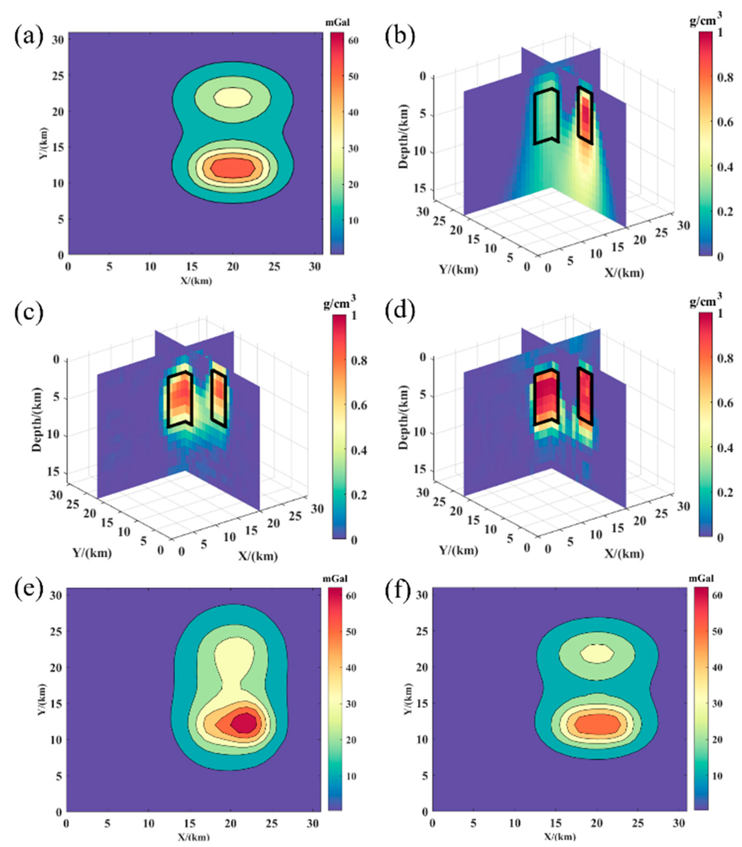
Figure 3a depicts a single prism with dimensions of 8 × 6 × 6 km. Figure 4b–d illustrate the inversion results of the traditional regularization inversion method, data-driven deep-learning method, and the constrained deep-learning method, respectively, where the solid black lines are the boundaries of the actual model. The traditional regularization inversion method is based on strict forward modeling theory so that the forward data-fitting difference corresponding to its inversion results meets the measurement accuracy requirements and has a high data-fitting accuracy. However, due to the inherent low depth resolution of the potential field data, as shown in Figure 4b, there is a severe trailing phenomenon below the body in the inversion result, and the ability to recover the three-dimensional spatial position of the model is poor. The inversion results of the constrained deep-learning method and data-driven deep-learning method are significantly better than that of the traditional regularization inversion method. However, in recovering the physical property parameters for the target body and delineating the three-dimensional position, the constrained deep-learning method can obtain a more focused three-dimensional distribution result of the physical property due to the constraints of the physical information. Figure 4e,f show the forward data for both methods. Due to the addition of data-fitting constraints, the constrained deep-learning method obtains a better data-fitting accuracy.

3.2.2. Model II

A horizontal adjacent superimposed prisms model is shown in Figure 3b. The horizontal adjacent superimposed prisms model consists of two identical prisms, each with dimensions of length 8 km, width 4 km, and height 6 km. There is a depth difference of 2 km between the prisms, and they are situated 6 km apart in the Y direction. Figure 5b–d display the inversion results of the traditional regularization inversion method, data-driven deep-learning method, and the constrained deep-learning method, respectively. The traditional regularization inversion result can invert the general position of the shallow prism but there is still a severe trailing phenomenon. However, the deep prism is wildly divergent and cannot invert the body’s spatial location and physical property distribution. The data-driven deep-learning method and the constrained deep-learning method can invert the three-dimensional space positions of the two adjacent superimposed prisms. However, the inversion results show that the constrained deep-learning method has a better result in delineating the density distribution parameter and boundaries due to the addition of physical information constraints. It indicates that the constrained deep-learning method exhibits a greater accuracy and resolution. In terms of forward data fitting, due to the addition of data-fitting terms, the fitting degree of the constrained deep-learning method is also much better than that of the data-driven deep-learning method, which makes the result obtained by the deep-learning inversion method with physical information constraints more consistent with the potential field forward theory.
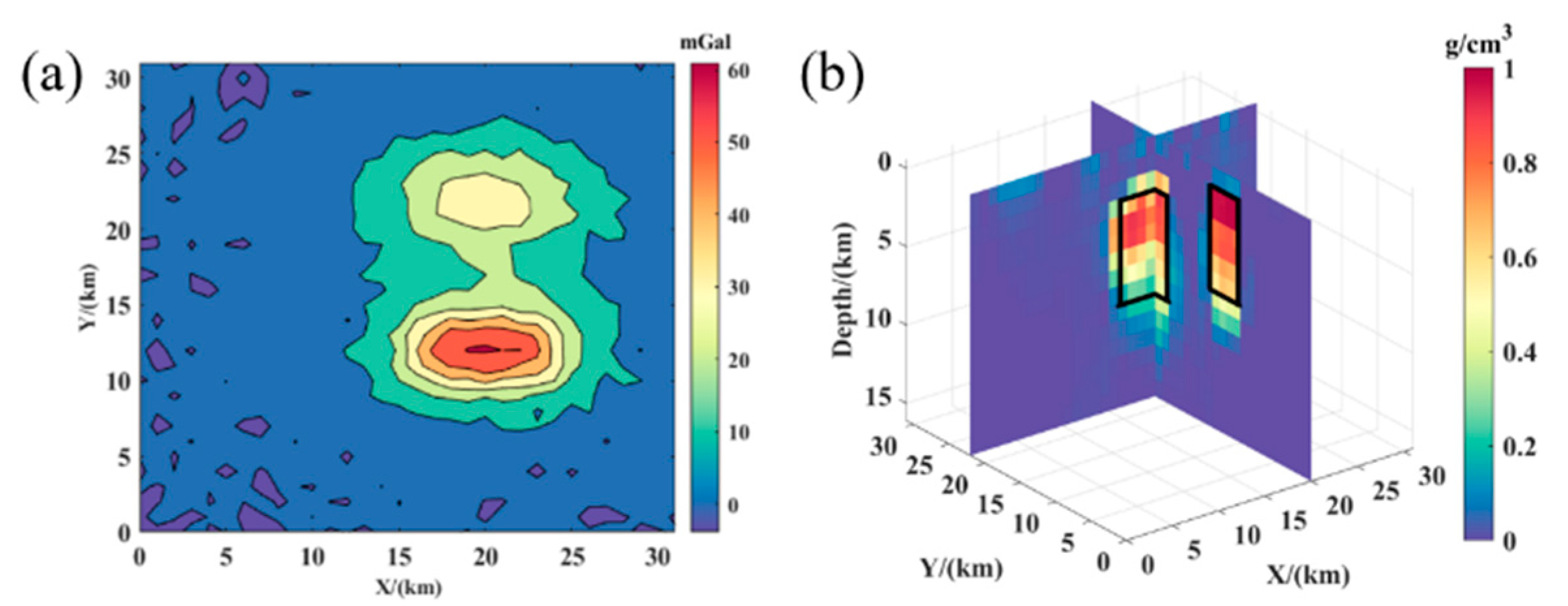
At the same time, in order to verify the anti-noise performance of the improved deep-learning method, 3% Gaussian noise is added to the real anomaly data shown in Figure 5a, and then input into the network for inversion as shown in Figure 6a. The inversion result is shown in Figure 6b. It can be noticed that noise has little influence on the inversion result, and the inversion result still has a good effect on the characterization of the density distribution parameter, indicating that the method has good noise resistance.

3.2.3. Model III

Figure 3c illustrates that the inclined steps model is comprised of two inclined steps with identical shapes but opposite orientations. One inclined step is made up of four small prisms, each measuring 8 km in length, 4 km in width, and 2 km in height, summing up to a total of 20 km for the entire structure. The two parts are at the same depth, are positioned opposite to each other along the Y direction, and are separated by a distance of 8 km along the X direction. Figure 7b–d show the inversion results of the traditional regularization inversion method, data-driven deep-learning method, and the constrained deep-learning method, respectively. The traditional regularization inversion method cannot invert the tilt trend of the target body without prior information constraints, and it can only invert the density parameter distribution of the top position of the target body. However, the inverse value of the physical property parameter is low, and there are a few parts with density values greater than 0.5 g/cm3. Therefore, the result shows the density values greater than 0.3 g/cm3.
Both the data-driven deep-learning method and the constrained deep-learning method can obtain the model’s incline information. However, the inversion results indicate that the constrained deep-learning method more closely aligns with the true boundary delineation. This approach exhibits a higher boundary fitting accuracy in both the upper and lower boundary of the target, attributable to the constraints imposed by the depth-weighting function. The inversion result of the constrained deep-learning method is also significantly better than that of the data-driven deep-learning method in terms of physical property parameter recovery, and the inversion density values are closer to the real density distribution. In terms of the data fitting, the fitting accuracy of the constrained deep-learning method is also significantly higher than that of the data-driven deep-learning method. This indicates that the constrained deep-learning method can effectively invert the underground inclined body, which has a good effect on model reconstruction and the outstanding performance in forward fitting.

3.2.4. Model IV

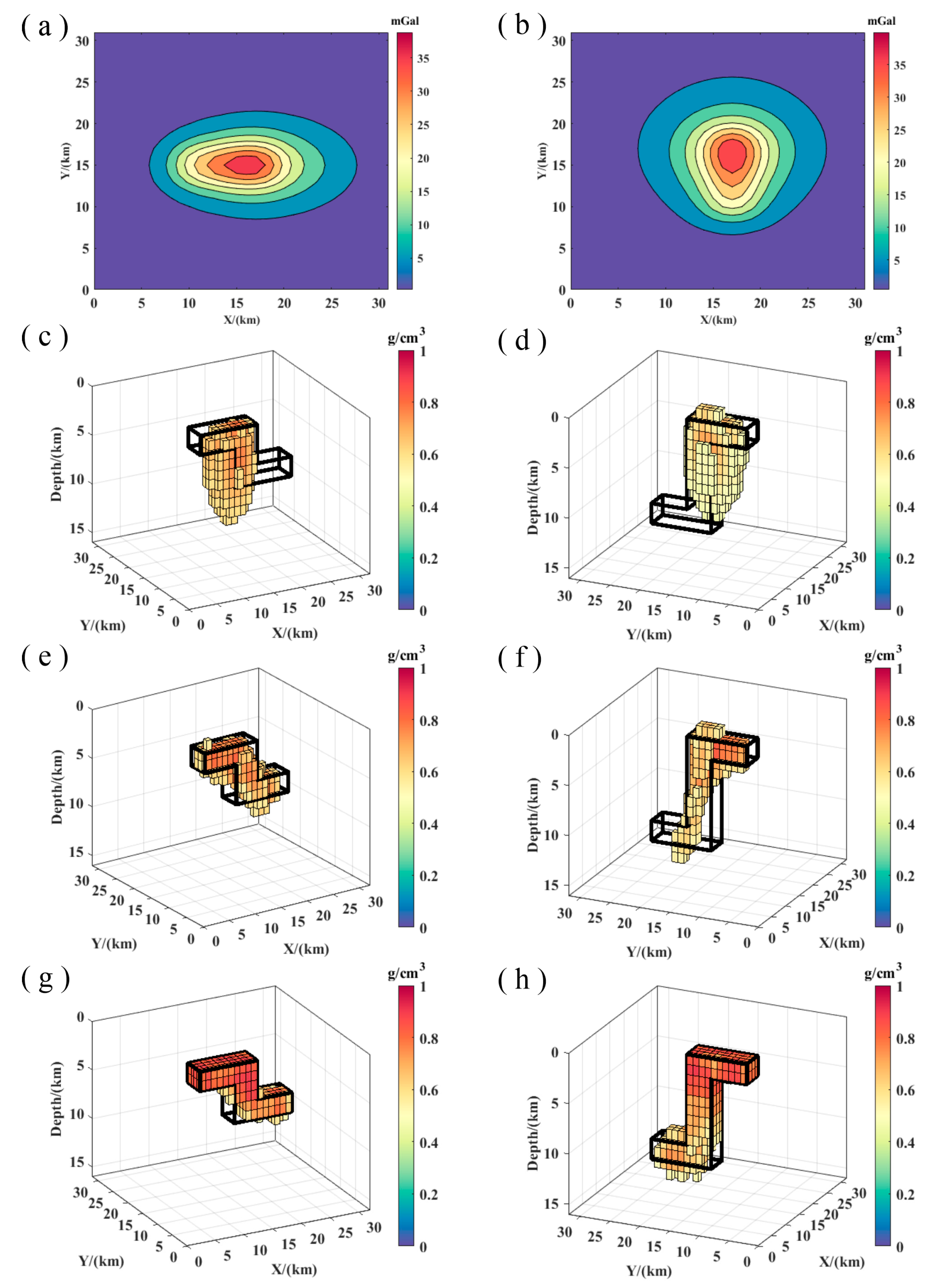
In order to illustrate the resolution in the depth direction constrained by the depth-weighting function, this paper establishes a model as shown in Figure 3d. The shape of the model is similar to the letter “Z”. Model I dimensions are 16 km in length, 4 km in width, and 6 km in height, whereas Model II extends 16 km in length, 4 km in width, and 11 km in height. Figure 8b–h illustrate the inversion results of the traditional regularization inversion method, data-driven deep-learning method, and the constrained deep-learning method of models I and II, respectively. The traditional regularization inversion method has a low depth resolution, and neither model I nor model II can invert the target body’s deep location physical property distribution. The data-driven deep-learning method has a good inversion effect on model I. However, the deep position resolution of model II is poor, and the physical property inversion effect is only good in the shallow part, indicating that the data-driven deep-learning method also has the problem of an insufficient depth resolution. However, due to the addition of physical information constraints, the inversion results of the constrained deep-learning method are good in the depth resolution of models I and II and have a smaller fitting difference.

3.2.5. Model V

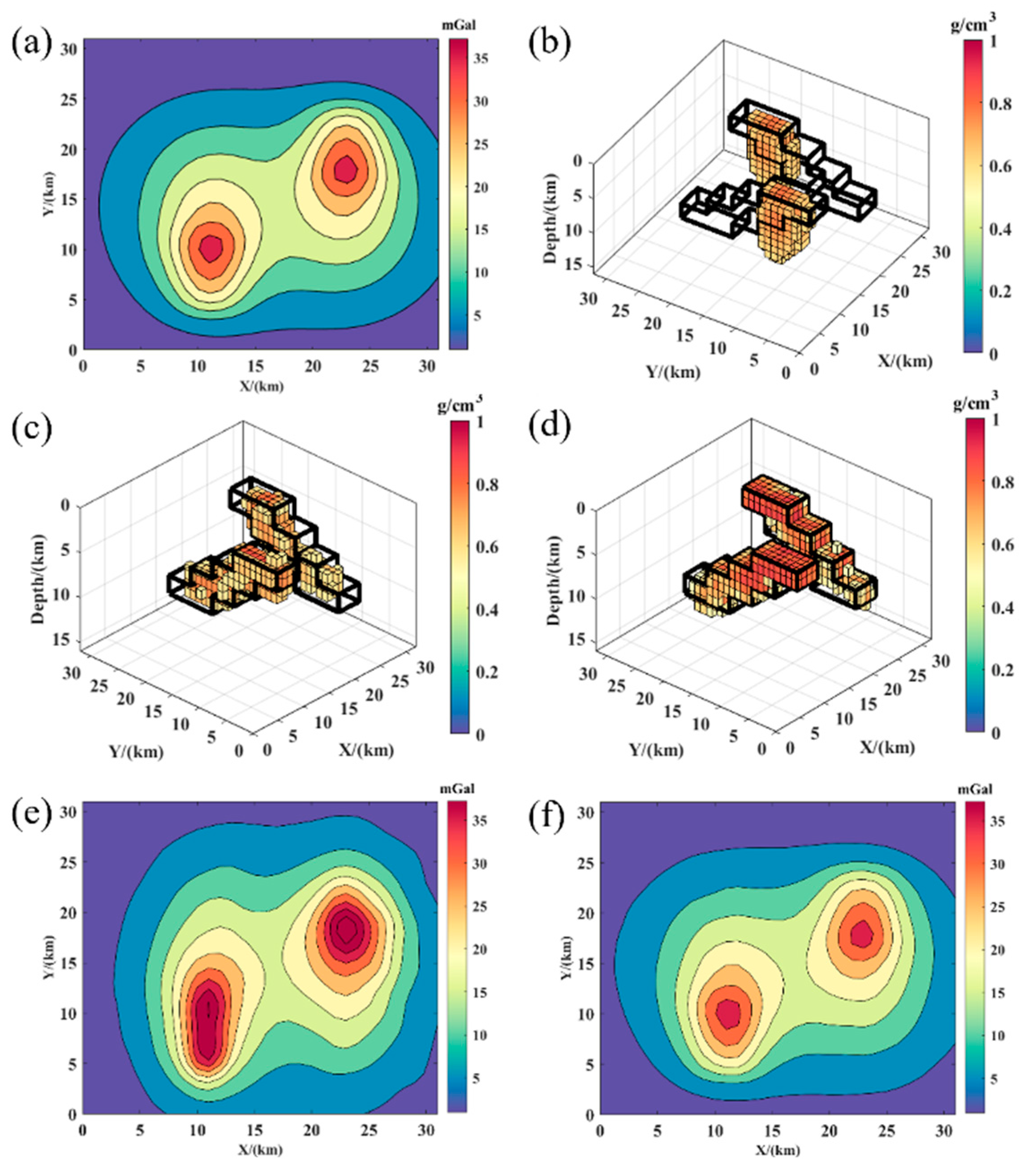
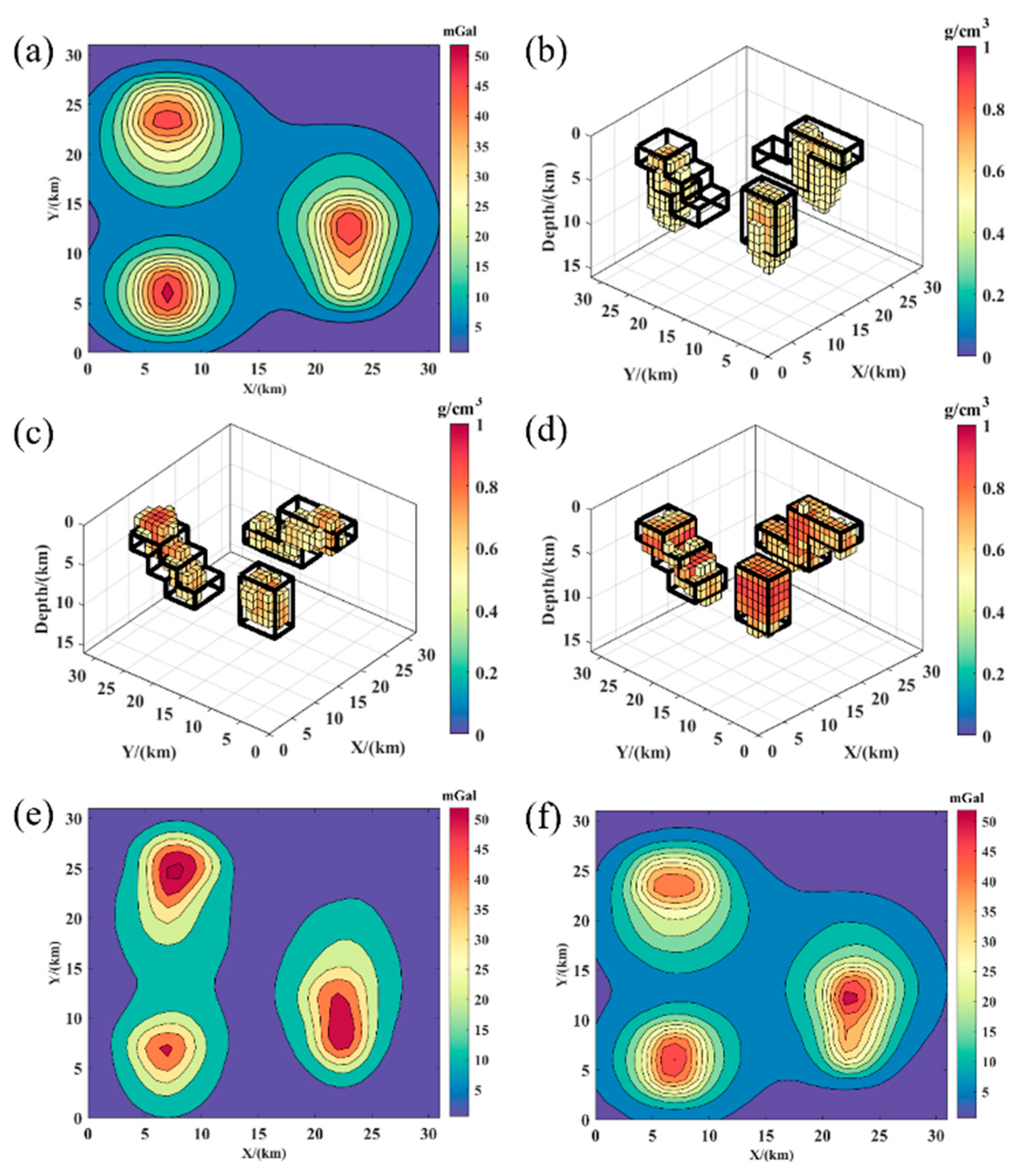
Figure 3e indicates that the complex combination model consists of a single prism, a three-step inclined step, and a Z-shaped model. Figure 9b–d display the inversion results of the traditional regularization method, the data-driven deep-learning method, and the constrained deep-learning method, respectively. When the model is complex, the constrained deep-learning method can still have a good effect, but the other two methods can only invert the model’s approximate position and have a poor effect on boundary fitting. In terms of forward fitting, since the model is complex, the fitting accuracy of the data-driven deep-learning method is inferior to that of the constrained deep-learning method.

3.3. Multi-Density Model

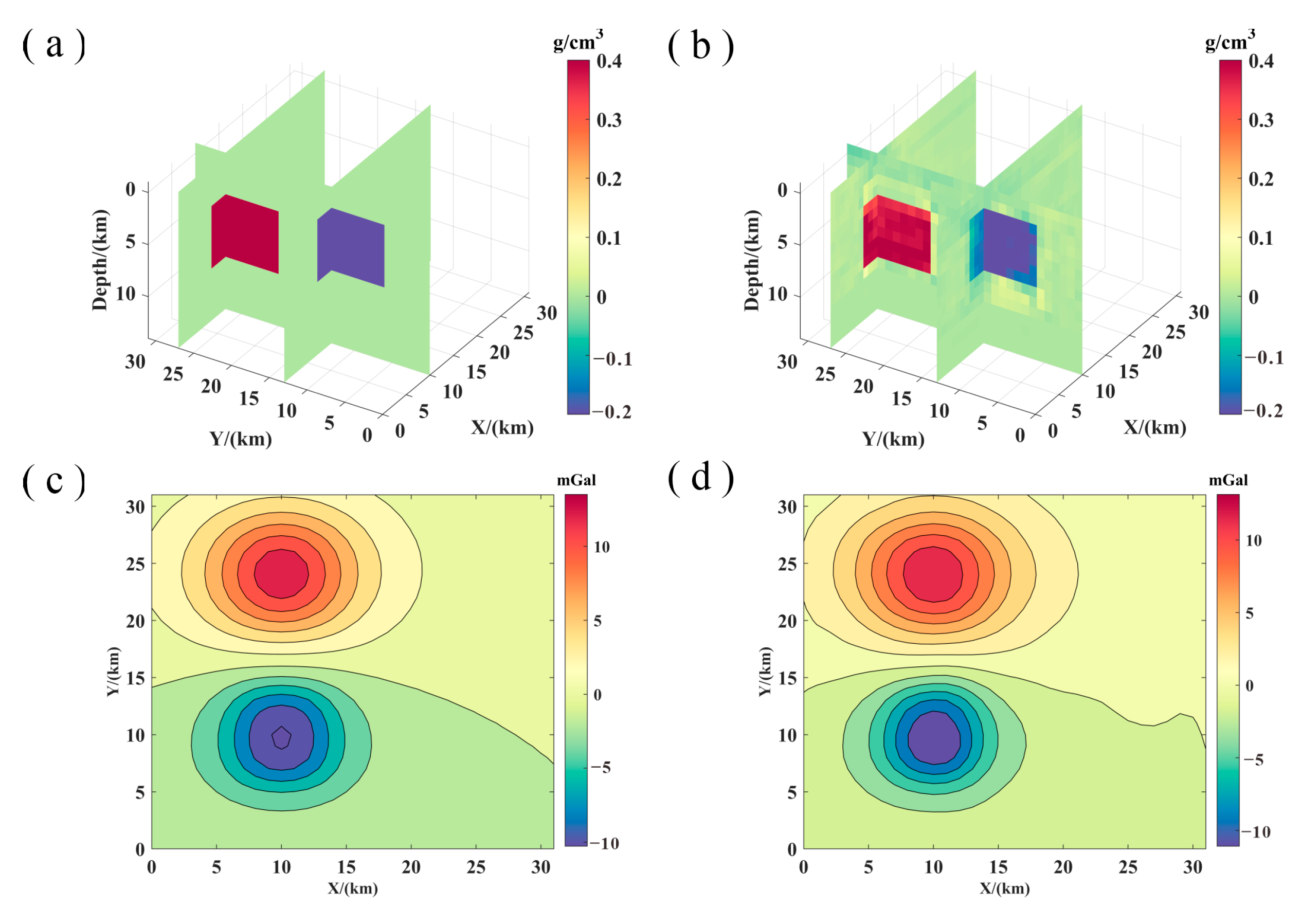
In practice, the underground anomalous bodies in the study area often have different density values. In order to discuss the practicability and effectiveness of the constrained deep-learning method in the above problems, the dataset is redesigned and trained. The new dataset is generated in a manner similar to the original method. The difference is that the density value of the original dataset is a constant value, while the density value of the new dataset contains several different density values with positive and negative values. After the training of the neural network, the inversion result as shown in Figure 10 is obtained. Figure 10a is a real model consisting of two prisms, one with a density value of 0.4 g/cm3 and the other with a density of −0.2 g/cm3. Figure 10b shows the inversion result. It can be seen that the method proposed in this paper is still applicable and effective when there are multiple different density values underground, and more accurate results can be obtained. Figure 10c,d are their forward data, and it can be seen that the forward-fitting accuracy of the inversion result is also high.

3.4. Analytical Metrics

To provide a more precise explanation of the inversion results, this study employs the root-mean-square error (RMSE) as a metric to quantitatively assess the discrepancy between the model and the data. The expression is as follows:
E m = 1 n i = 1 n m ^ m 2
E d = 1 n i = 1 n d ^ d 2
E m denotes the model fitting error and E d denotes data-fitting error, respectively. A value that is closer to zero signifies a more accurate model fitting and reduced error in data fitting. Subsequently, this paper conducts a quantitative analysis of the five aforementioned testing models, with the results presented in Table 1.

3.5. Ablation Experiment

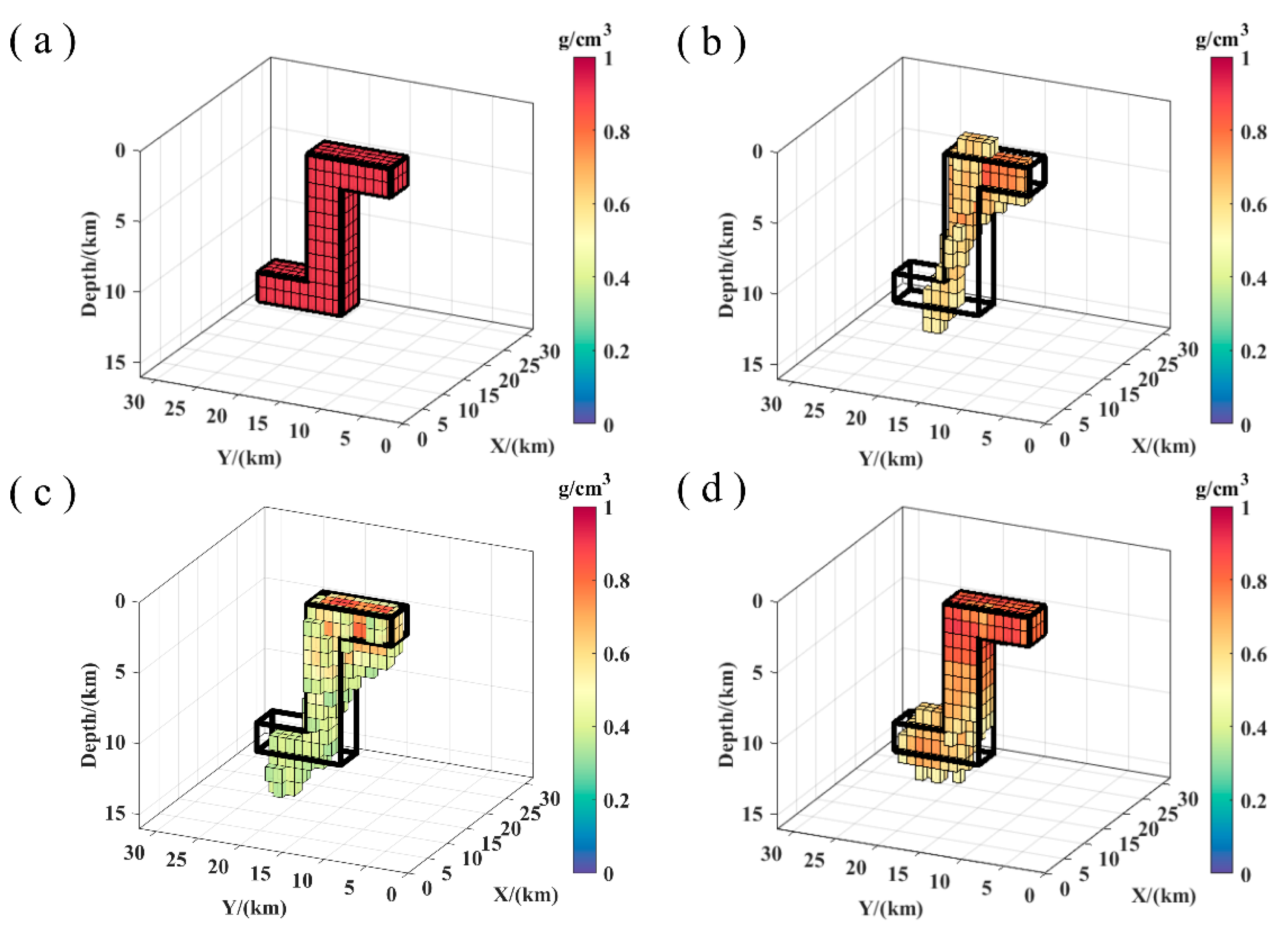
In order to confirm the role of the depth-weighting function in deep learning, a set of ablation experiments are also designed. As shown in Figure 11, Figure 11b–d are the results obtained by the inversion of only the model-fitting term, model-fitting and data-fitting terms, and model-fitting and data-fitting terms with depth weighting. By comparing Figure 11b,c, Figure 11c,d in pairs, the necessity of introducing the data-fitting term and depth-weighting function can be explained, respectively. At the same time, the quantitative error analysis is shown in Table 2, which can more intuitively see the effect of adding more information constraints. The result of Figure 11c is closer to the real model than that of Figure 11b, and has a higher fitting accuracy on the whole. Compared with Figure 11c, the result of Figure 11d has a more obvious improvement in depth resolution. In general, the addition of multiple constraint terms can provide more prior information for the inversion process, so as to obtain more accurate inversion results.

3.6. Regularization Parameter Selection

The selection of the regularization parameter plays a very important role in deep-learning network training [19,43]. At present, much of the parameter selection is empirical, requiring multiple tests to select the optimal parameter among multiple parameters [28,44]. To determine the appropriate regularization parameters for this article, we conducted the following research tests.
In order to select the optimal regularized parameter value, i.e., the α value, we select seven values distributed between 10−1 and 103. For each different regularization parameter value, we use the same data, parameters, and method for training, and test on a public testing dataset, and use quantitative analysis metrics to measure the error of the result. The test error obtained is shown in Figure 12. We can observe that the error reaches a minimum when the α is 100. Therefore, we choose α = 100 as the optimal value for the method in this paper.

4. Application of Actual Data

Geothermal resources are an important form of renewable and clean energy, which has a good performance as an alternative to conventional oil and gas resources. Hot dry rock resources are one of the most important geothermal resources with abundant reserves. It is typically found at depths of 3–10 km, where the reservoir temperature is above 150 °C. The Gonghe Basin is situated in the area where the geothermal activity is concentrated, and the geothermal anomaly is obvious. The research indicates that the average geothermal gradient in the Gonghe Basin is greater than double that of the standard geothermal gradient [45]. The Gonghe Basin is a region abundant in hydrothermal geothermal resources and also holds significant potential for the development of hot dry rock geothermal energy. In 2017, hot dry rock drilled 3705 m below well GR1 had a temperature of 236 °C, indicating the great exploration potential of geothermal energy from hot dry rocks in the Gonghe Basin [46].
A magnetotelluric survey is a passive electromagnetic geophysical method, which is very sensitive to the change in resistivity with depth and can effectively detect the underground resistivity structure. Partial melting or high-temperature anomalies are associated with electrical conductivity anomalies [47]. Therefore, this method is often used in the field of geothermal exploration, which can locate potential geothermal targets underground. Gao et al. conducted 3D magneto-electromagnetic measurements in the Gonghe area to determine the subsurface resistivity structure of the basin [48]. The obtained underground 3D resistivity model is shown in Figure 13.
As can be seen from Figure 13, there is a significant wide range of low-resistivity anomalies in the subsurface 15–35 km. This part can be reasonably inferred as the low resistivity caused by partial melting, which is the heat source of the Gonghe geothermal system.
It is widely recognized that increased temperatures lead to a reduction in both the seismic velocity and density of rocks [48]. The gravity anomaly mainly reflects the density difference of the underground rock. Therefore, three-dimensional gravity inversion can be effectively applied in the field of geothermal exploration. Justus Maithya used gravity data to explore the Eburru basin and successfully delineated the geological framework governing the geothermal system within the region, providing a basis for the geothermal exploration in the area [49].
For convenience, the data were processed in this study, including projection conversion, interpolation, etc. The satellite gravity data of the studied area after processing are shown in Figure 14.
According to the satellite gravity data, the appropriate parameters are selected again, and then the constrained deep-learning method is used for training. After the trained network is obtained, the prediction results of the underground density distribution in the study area can be obtained by using the gravity data as input. To present the inversion results more clearly, four slices are selected at different locations for display. The position of the slice is shown by the dotted line in Figure 15a, and the inversion results are shown in Figure 15b–e.
The inversion results indicate a broad distribution of low-density masses beneath the surface. This corresponds to the dominant low-density anomaly in the gravity anomaly, which confirms the reliability of the inversion results. Gao et al. used three-dimensional magnetotelluric imaging to invert the region and found low-resistivity anomalies at depths of 15–35 km [48]. It is inferred to be the heat source of the geothermal system in the Gonghe Basin. In the inversion results of our study, the depth of the low-density anomaly is about 10–35 km. This broadly conforms to the findings of Gao et al. [48]. Therefore, it is reasonable to conclude that, in Figure 15b–e, the black dotted line range is the heat source of the geothermal system, which may be high-temperature melt.

5. Conclusions

In this paper, we propose a deep-learning inversion method with physical information constraints. By introducing the data-fitting term and depth-weighting function into the loss function, the forward-fitting accuracy and depth resolution of the inversion results are improved and enhanced. In the model test, this research compares this method to the traditional regularization inversion and data-driven deep-learning inversion methods. It can be concluded, through a series of model tests from simple to complex, that the deep-learning inversion method proposed in this study is significantly superior to the other two methods in depth resolution and forward-fitting accuracy and has good generalization ability. At the same time, an anti-noise test is conducted on the proposed method. The results show that the method also has good robustness. Finally, the method proposed in this paper is applied to the field data, and reasonable results are obtained, which agree with the prior information, indicating that the method has the prospect of practical application.
However, this paper also has limitations. When the density of the dataset is set to a constant value, the trained network is not suitable for gravity anomalies caused by other density values. Therefore, the dataset should be designed with enough prior information so that the established dataset contains the density value of the target. In addition, in practical work, the density changes with the spatial position, such as the density changing with depth. However, the establishment of the dataset often ignores this point, so the application of the field data cannot obtain enough ideal results. Therefore, one of our future research directions is to impose constraints on the dataset, so that the dataset can meet more practical situations. In addition, we will continue to study how to apply additional physical information constraints to the network to achieve better results.

Author Contributions

Conceptualization, S.Z.; methodology, P.L.; writing, Y.W.; supervision, J.J.; project administration, H.J. All authors have read and agreed to the published version of the manuscript.

Funding

This work was supported in part by the Ningxia Key Research and Development Plan under Grant 2023BEG02066, in part by the Scientific Research Project of Education Department of Jilin Province under Grant JJKH20241293KJ, and in part by the Fundamental Research Funds for the Central Universities under Grant 2023-JCXK-15 and by the Engineering Research Center of Geothermal Resources Development Technology and Equipment, Ministry of Education, Jilin University.

Data Availability Statement

The original contributions presented in this study are included in the article. Further inquiries can be directed to the corresponding author.

Acknowledgments

The authors would like to thank the editors and reviewers for providing their valuable comments and suggestions.

Conflicts of Interest

The authors declare no conflicts of interest.

References

  1. Zhdanov, M.S. Inverse Theory and Applications in Geophysics; Elsevier: Amsterdam, The Netherlands, 2015. [Google Scholar]
  2. Jian, W.; Chongyang, S.; Hui, I.; Shaoan, S.; Lelin, X. Gravity inversion of deep-crust and mantle interfaces in the Three Gorges area. Geod. Geodyn. 2012, 3, 7–17. [Google Scholar] [CrossRef]
  3. Yang, G.; Wang, J.; Yan, H. Application of modeling inversion of Bouguer gravity anomalies to oil and gas exploration in the Erlian Basin. Chin. J. Geophys. 2019, 62, 316–330. [Google Scholar]
  4. Hinze, W.J. The role of gravity and magnetic methods in engineering and environmental studies. In Geotechnical an Environmental Geophysics: Volume I: Review and Tutorial; Ward, S.H., Ed.; SEG: Tulsa, OK, USA, 1990; pp. 75–126. [Google Scholar]
  5. Geng, M.; Huang, D.; Yang, Q.; Liu, Y. 3D inversion of airborne gravity-gradiometry data using cokriging. Geophysics 2014, 79, G37–G47. [Google Scholar] [CrossRef]
  6. Vatankhah, S.; Ardestani, V.E.; Renaut, R.A. Application of the χ2 principle and unbiased predictive risk estimator for determining the regularization parameter in 3-D focusing gravity inversion. Geophys. J. Int. 2015, 200, 265–277. [Google Scholar] [CrossRef]
  7. Li, Y.; Oldenburg, D.W. 3-D inversion of magnetic data. Geophysics 1996, 61, 394–408. [Google Scholar] [CrossRef]
  8. Li, Y.; Oldenburg, D.W. 3-D inversion of gravity data. Geophysics 1998, 63, 109–119. [Google Scholar] [CrossRef]
  9. Portniaguine, O.; Zhdanov, M.S. 3-D magnetic inversion with data compression and image focusing. Geophysics 2002, 67, 1532–1541. [Google Scholar] [CrossRef]
  10. Commer, M. Three-dimensional gravity modelling and focusing inversion using rectangular meshes. Geophys. Prospect. 2011, 59, 966–979. [Google Scholar] [CrossRef]
  11. Boulanger, O.; Chouteau, M. Constraints in 3D gravity inversion. Geophys. Prospect. 2001, 49, 265–280. [Google Scholar] [CrossRef]
  12. Pilkington, M. 3D magnetic data-space inversion with sparseness constraints. Geophysics 2009, 74, L7–L15. [Google Scholar] [CrossRef]
  13. Oldenburg, D.W.; Li, Y. Inversion for Applied Geophysics: A Tutorial. In Near-Surface Geophysics; Society of Exploration Geophysicists: Tulsa, OK, USA, 2005; pp. 89–150. [Google Scholar] [CrossRef]
  14. Namaki, L.; Gholami, A.; Hafizi, M.A. Edge-preserved 2-D inversion of magnetic data: An application to the Makran arc-trench complex. Geophys. J. Int. 2011, 184, 1058–1068. [Google Scholar] [CrossRef]
  15. Cheyney, S.; Fishwick, S.; Hill, I.A.; Linford, N.T. Successful adaptation of three-dimensional inversion methodologies for archaeological-scale, total-field magnetic data sets. Geophys. J. Int. 2015, 202, 1271–1288. [Google Scholar] [CrossRef]
  16. Rezaie, M. A sigmoid stabilizing function for fast sparse 3D inversion of magnetic data. Near Surf. Geophys. 2020, 18, 149–159. [Google Scholar] [CrossRef]
  17. Yang, Q.; Hu, X.; Liu, S.; Jie, Q.; Wang, H.; Chen, Q. 3-D Gravity Inversion Based on Deep Convolution Neural Networks. IEEE Geosci. Remote Sens. Lett. 2022, 19, 3001305. [Google Scholar] [CrossRef]
  18. Zhang, L.; Zhang, G.; Liu, Y.; Fan, Z. Deep Learning for 3-D Inversion of Gravity Data. IEEE Trans. Geosci. Remote Sens. 2022, 60, 5905918. [Google Scholar] [CrossRef]
  19. Wang, H.; Liu, Y.; Yin, C.; Su, Y.; Zhang, B.; Ren, X. Flexible and Accurate Prior Model Construction Based on Deep Learning for 2-D Magnetotelluric Data Inversion. IEEE Trans. Geosci. Remote Sens. 2023, 61, 5902511. [Google Scholar] [CrossRef]
  20. Qin, P.; Zhang, C.; Meng, Z.; Zhang, D.; Hou, Z. Three Integrating Methods for Gravity and Gravity Gradient 3-D Inversion and Their Comparison Based on a New Function of Discrete Stability. IEEE Trans. Geosci. Remote Sens. 2022, 60, 4505712. [Google Scholar] [CrossRef]
  21. Bhangale, K.B.; Kothandaraman, M. Survey of Deep Learning Paradigms for Speech Processing. Wirel. Pers. Commun. 2022, 125, 1913–1949. [Google Scholar] [CrossRef]
  22. Lin, Y.; Wu, Y. InversionNet: A real-time and accurate full waveform inversion with convolutional neural network. J. Acoust. Soc. Am. 2018, 144, 1683. [Google Scholar] [CrossRef]
  23. Ren, Y.; Nie, L.; Yang, S.; Jiang, P.; Chen, Y. Building Complex Seismic Velocity Models for Deep Learning Inversion. IEEE Access 2021, 9, 63767–63778. [Google Scholar] [CrossRef]
  24. Liu, Z.; Chen, H.; Ren, Z.; Tang, J.; Xu, Z.; Chen, Y.; Liu, X. Deep learning audio magnetotellurics inversion using residual-based deep convolution neural network. J. Appl. Geophys. 2021, 188, 104309. [Google Scholar] [CrossRef]
  25. Ren, Y.; Xu, X.; Yang, S.; Nie, L.; Chen, Y. A Physics-Based Neural-Network Way to Perform Seismic Full Waveform Inversion. IEEE Access 2020, 8, 112266–112277. [Google Scholar] [CrossRef]
  26. Li, Y.; Song, J.; Lu, W.; Monkam, P.; Ao, Y. Multitask learning for super-resolution of seismic velocity model. IEEE Trans. Geosci. Remote Sens. 2020, 59, 8022–8033. [Google Scholar] [CrossRef]
  27. Li, Y.; Jia, Z.; Lu, W. Self-Supervised Deep Learning for 3D Gravity Inversion. IEEE Trans. Geosci. Remote Sens. 2022, 60, 1–11. [Google Scholar] [CrossRef]
  28. Zhang, Z.; Lin, Y. Data-Driven Seismic Waveform Inversion: A Study on the Robustness and Generalization. IEEE Trans. Geosci. Remote Sens. 2020, 58, 6900–6913. [Google Scholar] [CrossRef]
  29. Puzyrev, V. Deep learning electromagnetic inversion with convolutional neural networks. Geophys. J. Int. 2019, 218, 817–832. [Google Scholar] [CrossRef]
  30. Wu, S.; Huang, Q.; Zhao, L. Convolutional neural network inversion of airborne transient electromagnetic data. Geophys. Prospect. 2021, 69, 1761–1772. [Google Scholar] [CrossRef]
  31. Liu, B.; Yu, A.; Yu, X.; Wang, R.; Gao, K.; Guo, W. Deep Multiview Learning for Hyperspectral Image Classification. IEEE Trans. Geosci. Remote Sens. 2021, 59, 7758–7772. [Google Scholar] [CrossRef]
  32. Bergen, K.J.; Johnson, P.A.; de Hoop, M.V.; Beroza, G.C. Machine learning for data-driven discovery in solid Earth geoscience. Science 2019, 363, eaau0323. [Google Scholar] [CrossRef]
  33. Wu, X.; Ma, J.; Si, X.; Bi, Z.; Yang, J.; Gao, H.; Xie, D.; Guo, Z.; Zhang, J. Sensing prior constraints in deep neural networks for solving exploration geophysical problems. Proc. Natl. Acad. Sci. USA 2023, 120, e2219573120. [Google Scholar] [CrossRef]
  34. Di, H.; Li, C.; Smith, S.; Li, Z.; Abubakar, A. Imposing interpretational constraints on a seismic interpretation convolutional neural network. Geophysics 2021, 86, IM63–IM71. [Google Scholar] [CrossRef]
  35. Kong, Q.; Wang, R.; Walter, W.R.; Pyle, M.; Koper, K.; Schmandt, B. Combining Deep Learning with Physics Based Features in Explosion-Earthquake Discrimination. Geophys. Res. Lett. 2022, 49, e2022GL098645. [Google Scholar] [CrossRef]
  36. Raissi, M.; Perdikaris, P.; Karniadakis, G.E. Physics-informed neural networks: A deep learning framework for solving forward and inverse problems involving nonlinear partial differential equations. J. Comput. Phys. 2019, 378, 686–707. [Google Scholar] [CrossRef]
  37. Rasht-Behesht, M.; Huber, C.; Shukla, K.; Karniadakis, G.E. Physics-Informed Neural Networks (PINNs) for Wave Propagation and Full Waveform Inversions. J. Geophys. Res. Solid Earth 2022, 127, e2021JB023120. [Google Scholar] [CrossRef]
  38. Wang, Y.; Wang, Q.; Lu, W.; Li, H. Physics-Constrained Seismic Impedance Inversion Based on Deep Learning. IEEE Geosci. Remote Sens. Lett. 2022, 19, 1–5. [Google Scholar] [CrossRef]
  39. Huang, R.; Liu, S.; Qi, R.; Zhang, Y. Deep Learning 3D Sparse Inversion of Gravity Data. J. Geophys. Res. Solid Earth 2021, 126, e2021JB022476. [Google Scholar] [CrossRef]
  40. Wang, Y.-F.; Zhang, Y.-J.; Fu, L.-H.; Li, H.-W. Three-dimensional gravity inversion based on 3D U-Net++. Appl. Geophys. 2021, 18, 451–460. [Google Scholar] [CrossRef]
  41. Hu, Z.; Liu, S.; Hu, X.; Fu, L.; Qu, J.; Wang, H.; Chen, Q. Inversion of magnetic data using deep neural networks. Phys. Earth Planet. Inter. 2021, 311, 106653. [Google Scholar] [CrossRef]
  42. Zhang, S.; Yin, C.; Cao, X.; Sun, S.; Liu, Y.; Ren, X. DecNet: Decomposition network for 3D gravity inversion. Geophysics 2022, 87, G103–G114. [Google Scholar] [CrossRef]
  43. Yang, Y.; Zhang, X.; Guan, Q.; Lin, Y. Making Invisible Visible: DataDriven Seismic Inversion with SpatioTemporally Constrained Data Augmentation. IEEE Trans. Geosci. Remote Sens. 2022, 60, 1–16. [Google Scholar]
  44. Celaya, A.; Denel, B.; Sun, Y.; ArayaPolo, M.; Price, A. Inversion of TimeLapse Surface Gravity Data for Detection of 3D CO2 Plumes via Deep Learning. IEEE Trans. Geosci. Remote Sens. 2023, 61, 1–11. [Google Scholar] [CrossRef]
  45. Liu, W.L. Drilling technical difficulties and solutions in development of Hot dry Rock geothermal energy. Adv. Pet. Explor. Dev. 2017, 13, 63–69. [Google Scholar]
  46. Zhang, C.; Jiang, G.; Jia, X.; Li, S.; Zhang, S.; Hu, D.; Hu, S. Parametric study of the production performance of an enhanced geothermal system, A case study at the Qiabuqia geothermal area, northeast Tibetan plateau. Renew. Energy 2018, 132, 959–978. [Google Scholar] [CrossRef]
  47. Samrock, F.; Kuvshinov, A.; Bakker, J.; Jackson, A.; Fisseha, S. 3-D analysis and interpretation of magnetotelluric data from the Aluto-Langano geothermal field, Ethiopia. Geophys. J. Int. 2015, 202, 1923–1948. [Google Scholar] [CrossRef]
  48. Gao, J.; Zhang, H.; Zhang, S.; Chen, X.; Cheng, Z.; Jia, X.; Li, S.; Fu, L.; Gao, L.; Xin, H. Three-dimensional magnetotelluric imaging of the geothermal system beneath the Gonghe Basin, Northeast Tibetan Plateau. Geothermics 2018, 76, 15–25. [Google Scholar] [CrossRef]
  49. Maithya, J.; Fujimitsu, Y.; Nishijima, J. Analysis of gravity data to delineate structural features controlling the Eburru geothermal system in Kenya. Geothermics 2020, 85, 101795. [Google Scholar] [CrossRef]
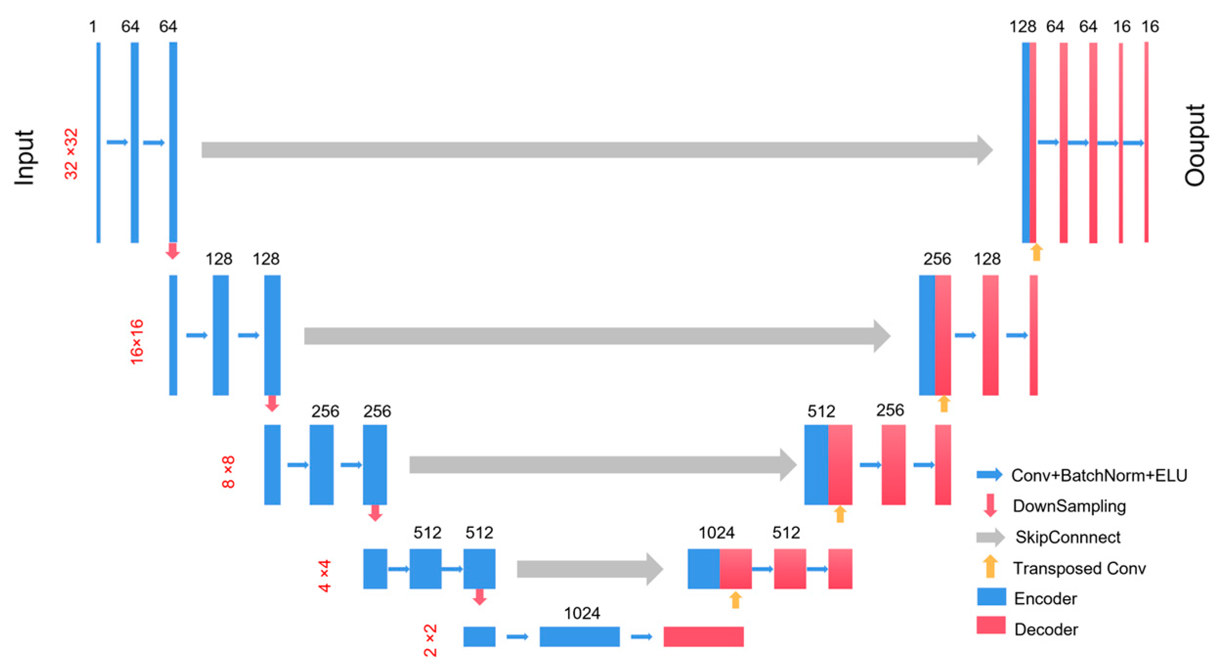
Figure 1. Schematic diagram of the network structure.
Remotesensing 16 04467 g001
Figure 2. The models in the training set. (a,b) one starting point, (c,d) two starting points.
Remotesensing 16 04467 g002
Figure 3. Three-dimensional distribution and parameters of the test model. (a) single prism model, (b) horizontal adjacent superimposed prisms model, (c) inclined steps model, (d) Z-shaped model, (e) complex combination model.
Remotesensing 16 04467 g003
Figure 4. Inversion results and forward anomaly maps of single-prism model: (a) real anomaly data; (bd) inversion results of the traditional regularization method, the data-driven deep-learning method, and the constrained deep-learning method; and (e,f) forward data of inversion result of the data-driven deep-learning method and the constrained deep-learning method.
Remotesensing 16 04467 g004
Figure 5. Inversion results and forward anomaly maps of horizontal adjacent superimposed prisms model: (a) real anomaly data; (bd) inversion results of the traditional regularization method, the data-driven deep-learning method, and the constrained deep-learning method; and (e,f) forward data of inversion result of the data-driven deep-learning method and the constrained deep-learning method.
Remotesensing 16 04467 g005
Figure 6. Noisy data and its inversion result: (a) anomaly data with 3% Gaussian noise; and (b) inversion result of the constrained deep-learning method.
Remotesensing 16 04467 g006
Figure 7. Inversion results and forward anomaly maps of inclined steps model: (a) real anomaly data; (bd) inversion results of the traditional regularization method, the data-driven deep-learning method, and the constrained deep-learning method; and (e,f) forward data of inversion result of the data-driven deep-learning method and the constrained deep-learning method.
Remotesensing 16 04467 g007
Figure 8. Inversion results and forward anomaly maps of Z-shaped model: (a,b) real anomaly data of model I and II; (c) inversion result of the traditional regularization method on model I (density > 0.3); (e) inversion result of the data-driven deep-learning method on model I; (g) Inversion result of the constrained deep-learning method on model I; (d) inversion result of the traditional regularization method on model II (density > 0.3 g/cm3); (f) inversion result of the data-driven deep-learning method on model II; and (h) inversion result of the constrained deep-learning method on model II.
Remotesensing 16 04467 g008
Figure 9. Inversion results and forward anomaly maps of complex combination model: (a) real anomaly data; (bd) inversion results of the traditional regularization method, the data-driven deep-learning method, and the constrained deep-learning method; and (e,f) forward data of inversion result of the data-driven deep-learning method and the constrained deep-learning method.
Remotesensing 16 04467 g009
Figure 10. Inversion result and forward data of multi-density model: (a) the real model; (b) the inversion result (absolute value of density > 0.1 g/cm3); and (c,d) their forward data.
Remotesensing 16 04467 g010
Figure 11. Ablation experiment: (a) the real model; (b) the inversion result of the data-driven method; (c) the inversion result of adding the data-fitting term; and (d) the inversion result of adding the depth-weighting function. (All results show parts with densities greater than 0.3.)
Remotesensing 16 04467 g011
Figure 12. Test error of different regularization parameters.
Remotesensing 16 04467 g012
Figure 13. 3D magnetotelluric imaging results (modified from [48]).
Remotesensing 16 04467 g013
Figure 14. Satellite gravity data in the study area.
Remotesensing 16 04467 g014
Figure 15. Profile (be) along the white dotted line in (a).
Remotesensing 16 04467 g015
Table 1. Error analysis of the models. Methods I, II, and III are traditional regularization method, data-driven deep-learning method, and the constrained deep-learning method.
ModelMethod IMethod IIMethod III
EmEdEmEdEmEd
single prism27.08800.01028.888160.02255.952317.8810
horizontal adjacent superimposed prisms26.08420.009911.426497.76627.707717.7445
inclined steps 25.94570.009515.407593.136410.752612.5255
Z-shaped modelI17.2367
11.9710
0.0088
0.0099
8.8974
11.5936
47.4270
61.2051
5.9650
7.8873
9.1144
9.7404
II
complex combination model30.28150.460816.0528154.209712.030439.3747
Table 2. Error analysis of ablation experimental models.
ModelEmEd
Figure 11b11.593661.2051
Figure 11c11.044133.1886
Figure 11d7.88739.7404
Disclaimer/Publisher’s Note: The statements, opinions and data contained in all publications are solely those of the individual author(s) and contributor(s) and not of MDPI and/or the editor(s). MDPI and/or the editor(s) disclaim responsibility for any injury to people or property resulting from any ideas, methods, instructions or products referred to in the content.