Article

Optimal-Transport-Based Positive and Unlabeled Learning Method for Windshear Detection

1
Department of Mathematics, The University of Hong Kong, Pokfulam, Hong Kong
2
Aviation Weather Services, Hong Kong Observatory, Kowloon, Hong Kong
3
Department of Mathematics, Hong Kong Baptist University, Kowloon Tong, Hong Kong
*
Author to whom correspondence should be addressed.
Remote Sens. 2024, 16(23), 4423; https://doi.org/10.3390/rs16234423
Submission received: 15 October 2024 / Revised: 11 November 2024 / Accepted: 22 November 2024 / Published: 26 November 2024

Abstract

:
Windshear is a microscale meteorological phenomenon that can be dangerous to aircraft during the take-off and landing phases. Accurate windshear detection plays a significant role in air traffic control. In this paper, we aim to investigate a machine learning method for windshear detection based on previously collected wind velocity data and windshear records. Generally, the occurrence of windshear events are reported by pilots. However, due to the discontinuity of flight schedules, there are presumably many unreported windshear events when there is no flight, making it difficult to ensure that all the unreported events are all non-windshear events. Hence, one of the key issues for machine-learning-based windshear detection is determining how to correctly distinguish windshear cases from the unreported events. To address this issue, we propose to use a positive and unlabeled learning method in this paper to identify windshear events from unreported cases based on wind velocity data collected by Doppler light detection and ranging (LiDAR) plan position indicator (PPI) scans. An optimal-transport-based optimization model is proposed to distinguish whether a windshear event appears in a sample constructed by several LiDAR PPI scans. Then, a binary classifier is trained to determine whether a sample represents windshear. Numerical experiments based on the observational wind velocity data collected at the Hong Kong International Airport show that the proposed scheme can properly recognize potential windshear cases (windshear cases without pilot reports) and greatly improve windshear detection and prediction accuracy.

1. Introduction

Windshear is a sustained change in wind velocity [1] that can suddenly change the lift force experienced by an aircraft. Significant windshear can cause aircraft to fly above or below the intended flight path, making it difficult for pilots to safely control aircraft. Therefore, accurate windshear alerts can help pilots take appropriate corrective and timely actions during flight, making this type of alert important for air traffic control.
Windshear is caused by various factors, such as microbursts, convection, frontal systems, and thermal instabilities [2]. Windshear can occur on both non-rainy and rainy days for different reasons [3]. Microbursts and gust fronts associated with windshear can occur in rainy weather conditions and can be detected by rain-detecting Doppler weather radar and anemometers. On non-rainy days, terrain effects, sea breezes, and low-level jets are the leading causes of windshear. However, there are few reflectors for microwaves in clear air, which makes it challenging to obtain adequate wind velocity data from Doppler weather radar under non-rainy weather conditions. With the development of light detection and ranging (LiDAR) techniques [4,5], Doppler weather LiDAR is used as a new remote sensing instrument for dry windshear detection.
In general, windshear detection methods are mainly based on several indicators related to flight conditions and the statistical properties of wind velocity data, e.g., the wind ramp and F-factor. Wind ramp [6,7] is the change in the wind velocity along a certain distance (ramp length). In [1], Chan et al. proposed detecting wind ramps with several different ramp lengths ( 400 , 800 , , 6400 m) and then selecting some of these wind ramps via ramp prioritization based on a severity factor corresponding to the ratio between the inverse cube root of the related ramp length and the change in the wind velocity. If any of the selected ramps reaches or exceeds 14 knots, a windshear alert is generated. However, this approach ignores the internal characteristics of the wind ramp waveform that may reflect the pilots’ insights. To adapt the intuition of pilots, Li et al. [5] proposed a novel ramp algorithm that includes a ramp detection method involving weighted signal smoothing and a secondary windshear recognition scheme. Hon et al. proposed a “gentle ramps” removal method for the same purpose in [8], in which an additional check based on the root-mean-square (RMS) of the original headwind profile from its running mean is applied to suppress the windshear alerts generated by wind ramps with low-velocity fluctuations. In addition to wind ramp, F-factor [9] is another widely used indicator in windshear detection. It is more advantageous than wind ramp as an indicator in some cases as it takes the headwind gradient into account. In [10], Chan et al. applied the F-factor algorithm in low-level windshear alerting; this approach could capture approximately 87 % to 90 % of windshear with a proper choice for the F-factor alert threshold. However, these researchers did not investigate the vertical acceleration term of the F-factor and the aircraft response to the headwind change. In [11], the aircraft response is included in the F-factor-based method by preprocessing the headwind profile using commercial flight simulator software. Further research is shown in [12], where both the flight-simulator-based F-factor and center-averaging F-factor approaches are studied. The successful alerting rate of the proposed method could reach 86 % with an optimal alerting threshold specific for each runway corridor. In addition to detection methods based on wind ramp and F-factor, other methods have been applied. In [13], Wu et al. applied a spectral decomposition based on Fourier transformation to decompose the headwind profile into components with different length scales and detected windshear via a threshold-based approach. Li et al. [14] proposed a regional divergence algorithm based on LiDAR data for windshear detection at Lanzhou Zhongchuan International Airport that can evaluate the extent of regional wind changes along the runway.
Over the past few years, several machine-learning-based windshear detection methods have been proposed with the development of machine learning. Ma et al. [15] proposed a support vector machine (SVM) learning method based on the windshear features extracted from partial LiDAR scanning images via a gray-gradient co-occurrence matrix and invariant moment method. However, the accuracy of this method is lower than 50 % in practice, which is quite poor. In [16], Huang et al. proposed two statistical indicators based on the maximal difference in wind velocities within a range of azimuth angles. A one-side normal-distribution-based decision rule is applied to determine the threshold of the proposed indicators for windshear detection. The accuracy of this method is greater than 90 % . To our knowledge, this is the best existing method for windshear detection using machine learning based entirely on LiDAR wind velocity data. However, this method takes only the wind velocity data collected at the timestamp nearest to the reported time spot, which might cause windshear feature loss in practice. Additionally, high requirements are placed on the selection of training datasets. Suppose we simply select the non-reported cases as negative samples in model training. In that case, the detection performance of this method might not be satisfactory as there are some non-reported windshear cases (i.e., mislabeled samples in the negative dataset).
In this study, we aim to train a binary classifier for windshear detection from the LiDAR observational wind velocity data. In contrast to previous learning-based windshear detection methods, in which windshear is detected by a classifier trained via supervised learning, we propose a positive and unlabeled learning (PUL) model for windshear detection, in which the features collected at the pilots’ reported timestamps can be regarded as positive samples while features collected at other timestamps are unlabeled samples. This approach is more applicable than the supervised learning method as we can ensure only that there is windshear during the flight time according to the pilot reports and cannot determine whether there is windshear during the non-flight time. Specifically, an optimal transport (OT)-based model without any prior information on the distribution of unlabeled samples is developed to predetermine the labels of these samples. Then, a binary classifier can be developed via some supervised machine learning methods, such as the support vector machine (SVM) method, linear discriminant analysis (LDA) method, and k-nearest neighbor (KNN) method, for windshear and non-windshear classification. Moreover, unlike the previous feature extraction methods that consider only the features extracted by the wind velocity data observed at the timestamp nearest to the reported time, we extract the windshear features from the wind velocity data collected over several minutes (4 min in this paper) around the investigated timestamp via multiple instance learning. Numerical results on the LiDAR velocity data collected at the Hong Kong International Airport (HKIA) show that the proposed method effectively identifies potential windshear cases (windshear cases without pilot reports) and detects windshear.
The outline of this paper is as follows. The second section briefly introduces optimal transport and the methods of positive and unlabeled learning. Then, the details of the proposed learning scheme are introduced in Section 3. Numerical experiments on the LiDAR wind velocity data collected at HKIA and corresponding discussions are shown in Section 4. Finally, some concluding remarks are given in Section 5.

2. Optimal Transport and Positive and Unlabeled Learning

2.1. Optimal Transport

Optimal transport (OT) is a mathematical problem that aims to define geometric tools for different probability distribution comparisons. OT was first proposed by Monge in the 18th century [17], then modified by Kantorovich in [18]. For the fast computation of OT problems, Cuturi [19] introduced negative entropy regularization to the original OT problem and proposed a Sinkhorn fixed-point algorithm to find the solution. Then, a series of fast computational algorithms for the negative-entropy-regularized OT problem were proposed in the literature [20,21,22].
With the development of efficient algorithms, OT has been widely used to estimate the distance between two probability distributions [23,24,25]. The earth movers’ distance (EMD), which is defined based on optimal transport, is used in multiple instance learning to evaluate the difference between two bags in [26]. Based on the Wasserstein distance, Wasserstein discriminant analysis has been implemented for supervised learning [27,28,29]. To stabilize the training of generative adversarial networks, the Wasserstein distance is introduced into the generative models [30,31]. Moreover, optimal transport can be applied to match two distributions. Courty et al. [32] applied optimal transport to domain adaptation to improve supervised learning performance in different domains, which transports the source samples to the same distribution of target samples with the minimal transport cost to reduce the distribution discrepancy between the investigated domains. The label information of data was further leveraged based on this for different label-conditional distributions in [33]. Zhang et al. extended the application of optimal-transport-based distribution matching to the reproducing kernel Hilbert space (RKHS) in [34]. Recently, some researchers have applied optimal transport methods to positive and unlabeled learning [35,36] to predetermine the labels of unlabeled samples based on the optimal transport plan for sequential supervised learning.

2.2. Positive and Unlabeled Learning
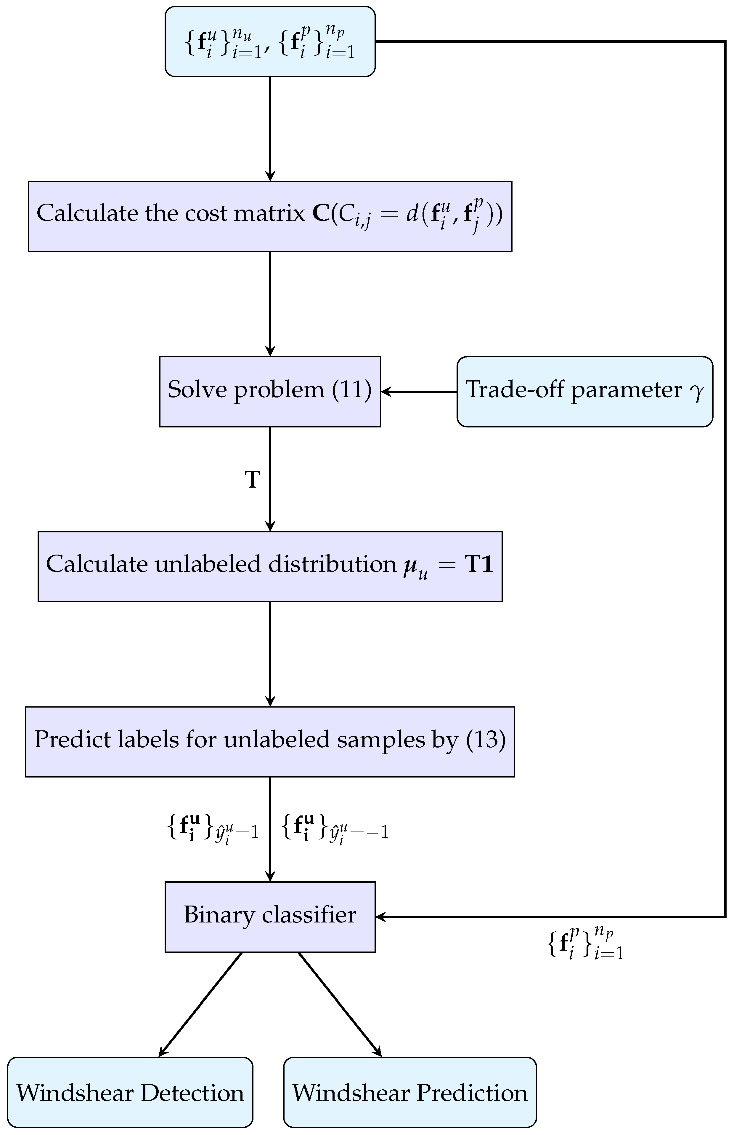
Positive and unlabeled learning (PUL) is a notable topic in machine learning [37]; this approach aims to train a binary classifier on only positively labeled samples and samples without any prior label information. It can be widely applied in many areas, such as biology science [38], medical diagnosis [39], computer vision [40], and fake news detection [41,42].
To address the challenges associated with the absence of negative samples, several strategies have been proposed in the literature. Some of the earliest methods aim to recognize reliable negative samples from the unlabeled data and then train a binary classifier based on the distinguished positive and negative samples [43,44]. With the development of label denoising, methods based on label denoising were proposed [45,46], treating all the unlabeled training data as negative samples with label noise and estimating the centroid of negative samples by reducing the impact of label noise. However, neither of these works considered the distribution information of the training samples. Recently, inspired by the optimal transport property [23,32], which can be used to extract the data distribution information, several optimal-transport-based positive and unlabeled learning methods have been proposed. There are two main kinds of methods for applying optimal transport to positive and unlabeled learning. The first kind of method [47] treats all the unlabeled samples as negative samples and allocates an entropy weight to each sample based on the entropic optimal transport plan for corresponding weighted classifier training. The other kind of method first predetermines the labels for unlabeled samples via optimal transport and then trains a supervised classifier by using the learned labels. For instance, in [35], a partial optimal transport model was proposed and applied to positive and unlabeled learning. Cao et al. [36] applied entropy-regularized optimal transport to achieve a much more precise estimation for class priors and then developed a label noise insensitive classifier for PUL by optimizing the margin distribution. Note that all of the above methods apply a fixed marginal distribution for the unlabeled samples, which might lead to misclassification in practice. In this paper, we propose to use an automatic mass distribution plan for unlabeled samples without any prior information on the optimal transport procedure and predetermine the labels of unlabeled samples based on the optimal transport plan.

3. Proposed Method

In this section, we introduce the proposed method for windshear detection. First, we introduce the information of the LiDAR observational data studied in this paper and corresponding pilots’ reports. Then, we provide a brief analysis of learning-based windshear detection. A brief introduction to windshear feature extraction is provided in the third part of this section. Finally, we show the proposed learning model and the corresponding optimization algorithm.

3.1. LiDAR Observational Data and Pilots’ Reports

In this paper, we mainly use LiDAR observational wind velocity data collected by PPI scans at HKIA in the springtime (February to April), when the prevailing wind direction is from the east to southeast. As Figure 1 shows, there are two Doppler LiDARs at HKIA, the north one of which scans for the north runway while the south one scans for the south runway. Both of them use the laser beam of 1.5 microns to track the movement of aerosols in order to determine the radial velocity of the wind, which can capture most of the windshear cases (windshear on non-rainy days) reported by pilots. Figure 2 shows an example of the investigated wind velocity data obtained by PPI scans at HKIA, where the negative wind velocities (blue/green/purple) denote the speeds of wind moving toward the LiDAR, and the positive wind velocities (yellow/pink/orange/ brown) denote the speeds of wind moving away from the LiDAR. Each scan takes approximately 20–30 s, and approximately 400–500 LiDAR beams are emitted for one scan.
According to Figure 2, there are two main areas in the region that cover the flight approach/departure corridors, i.e., the eastern area ( 10 150 ) for the tailwind velocities of aircraft and the western area ( 220 340 ) for the headwind velocities of aircraft. Due to the complex terrain near HKIA, many wind velocity values are missing at LiDAR points with a slant range larger than 4950 m. Hence, we extracted the windshear features from the wind velocity data collected at a slant range of 350 m–4950 m.
During flight, pilots would report to the air traffic control personnel when they encounter perilous meteorological circumstances, including the occurrence of windshear, which provides us a reliable reference to verify the effectiveness of proposed windshear detection methods. Specifically, the reports collected from pilots at HKIA are highly detailed, containing specific information about the timing, position, altitude, and magnitude of a windshear event. Here, to make our proposed method applicable to windshear events with less detailed reports, we consider only the timestamps of windshear occurrences. A positive label is assigned to a feature vector if it is extracted from wind velocity data collected during the time reported by the pilot.

3.2. Analysis of Learning-Based Windshear Detection

There are three main difficulties in the development of learning-based windshear detection:
(i)
We do not know the exact location and range of windshear occurrence, making it challenging to explicitly extract the windshear features from LiDAR observational wind velocity data. In other words, windshear features might be missed by inappropriate feature extraction methods. Hence, it could be better to extract the windshear features globally based on all the wind velocity data collected by LiDAR in the region that covers the flight path and touch-down zone. Details about the specific region discussed in this paper are provided in Section 3.1.
(ii)
Although windshear occurrence can be recorded by pilot reports, the exact onset time of windshear is unknown. Taking pilots’ recording delays in actual operations into account, the previous learning-based windshear detection methods that extract the windshear features from the wind velocity data collected at the timestamp nearest to the reported time spot might miss windshear features. It could be better to extract windshear features from all LiDAR observational wind velocity data collected several minutes around the reported time spot.
(iii)
We cannot determine whether windshear occurs during non-flight times. Namely, in the learning procedure, we have precise knowledge from some positive-labeled samples (i.e., windshear cases reported by pilots) but have no information for negative-labeled samples, constituting a positive and unlabeled learning problem.

3.3. Windshear Features

In this section, we briefly introduce several features extracted from the LiDAR observations of wind velocity that can indicate whether windshear occurs. For more details, please refer to [48].
Let x i = [ x i , 1 , x i , 2 , , x i , n ] R n be the wind velocity data observed by LiDAR PPI scan at azimuth angle θ i . For simplicity, we assume that there are k 1 azimuth angles ( θ 1 ( 1 ) < θ 2 ( 1 ) < < θ k 1 ( 1 ) ) for the collection of wind velocity data in the tailwind part and k 2 azimuth angles ( θ 1 ( 2 ) < θ 2 ( 2 ) < < θ k 2 ( 2 ) ) for the collection of wind velocity data in the headwind part. Additionally, there are m different slant range values for the collection of wind velocity data along a fixed azimuth angle, i.e.,
x i ( 1 ) = [ x i , 1 ( 1 ) , x i , 2 ( 1 ) , , x i , m ( 1 ) ] , 1 i k 1 ;
x i ( 2 ) = [ x i , 1 ( 2 ) , x i , 2 ( 2 ) , , x i , m ( 2 ) ] , 1 i k 2 .
Note that the locations of such range values are not necessarily uniform and that the distance between the LiDAR center and the observed point x i , j is equal to r j .
There are two main kinds of features extracted from the LiDAR observational wind velocity data: features derived from the physical property of windshear, and features obtained from the images of the LiDAR PPI wind velocity scans by image processing methods.
Based on the physical properties of windshear, the variation in wind velocity is used to evaluate the headwind/tailwind change in the investigated area. For a fixed azimuth angle θ i ( 1 ) ( θ i ( 2 ) ), the variation in the tailwind can be evaluated by the indicator
max 1 j m ( x i , j ( 1 ) ) min 1 j m ( x i , j ( 1 ) )
and the variation in the headwind can be estimated by
max 1 j m ( x i , j ( 2 ) ) min 1 j m ( x i , j ( 2 ) )
Based on experience, the top 12 maximum variations of each area are extracted to represent the change in the wind velocity, which are denoted as f p ( 1 ) and f p ( 2 ) , respectively. In the case of windshear, there are large wind velocity fluctuations, so the term with a larger L 2 norm in between f p ( 1 ) and f p ( 2 ) is selected as the indicator f p for the observed LiDAR scan, i.e.,
f p = f p ( 1 ) i f f p ( 1 ) 2 f p ( 2 ) 2 , f p ( 2 ) otherwise .
From the LiDAR PPI scan of wind velocity (e.g., Figure 1), some image texture features can be extracted by the gray level co-occurrence matrix (GLCM) method, which can also reflect the occurrence of windshear. Here, the dissimilarity, contrast, and correlation of the corresponding co-occurrence matrices are calculated as the statistical indicator f i m for the LiDAR PPI scan, the equations for which are given as follows:
Dissimilarity:
i , j = 0 255 p ( i , j ) | i j |
Contrast:
i , j = 0 255 p ( i , j ) ( i j ) 2
Correlation:
i , j = 0 255 p ( i , j ) ( i μ i ) ( j μ j ) ( σ i 2 ) ( σ j 2 ) ,
where μ i , μ j and σ i , σ j denote the mean values and standard deviation values, respectively.
Here,
p ( i , j ) = # { ( p 1 , p 2 ) I p 1 = i & p 2 = j } # I ,
denotes the co-occurrence probability for co-occurring pixels with gray levels i and j with specified interpixel distances and orientations in image I.
From the two indicators f p and f i m , we can construct several feature vectors from the LiDAR observational wind velocity data.

3.4. Learning Model

Based on the above analysis, we propose to develop a positive and unlabeled learning method for windshear detection. Here, we consider the LiDAR observational wind velocity data obtained for 4 min around the reported timestamp. Note that 6–11 LiDAR PPI scans could be collected for 4 min. In other words, we can obtain 6–11 feature vectors by the feature extraction methods described in Section 3.3. Inspired by the idea of multiple-instance learning [26], we propose considering these feature vectors at the “bag” level. The bag’s label would be set as positive as long as there are one or more windshear feature vectors. Specifically, after the extraction of windshear features from all the LiDAR PPI scans collected in the investigated 4 min, one feature vector is selected to represent the windshear feature obtained at the corresponding timestamp. Then, we can perform positive and unlabeled learning.
Mathematically, let x R d be the windshear feature vector extracted from the wind velocity data obtained by one LiDAR PPI scan, and let X = { x 1 , x 2 , , x n } be the set of windshear feature vectors for the LiDAR scans obtained in one period (four minutes around the investigated time stamp), i.e., one bag in multiple instance learning. The typical property of windshear is the change in wind speed and direction. There is a significant variation in the wind velocity when windshear occurs, while there is a slight variation in the wind velocity in non-windshear cases. Based on this and the feature extraction method for the wind velocity data obtained by each LiDAR scan, we propose using the feature vector that has the maximum L 2 -norm as the feature vector for bag X , i.e.,  f X = max 1 i n { x i } . Let y = ± 1 be the label of one bag (windshear case: y = 1 ; non-windshear case: y = 1 ). Assume that there are n p samples { f i p } i = 1 n p that are labeled as positive (i.e., feature vectors for pilot-reported windshear cases) among the training samples and n u samples { f i u } i = 1 n u whose labels are unknown. Then, let us consider the procedure of positive and unlabeled learning.
Let μ u and μ p denote the empirical distributions of the unlabeled training samples { f i u } i = 1 n u and positive-labeled samples { f i p } i = 1 n p , respectively. Based on the distribution information of training samples, we propose transporting unlabeled samples that are distributed close to known positive-labeled samples (i.e., potential positive-labeled samples) to positive-labeled samples by using optimal transport so that we can pre-classify the unlabeled samples.
Note that a transport plan T from unlabeled samples to labeled samples can be represented as a joint distribution of μ u and μ p that satisfies the following condition:
T 1 = μ u , T 1 = μ p ,
where 1 denotes a vector with all the elements being 1. The marginal distributions μ u and μ p indicate how many masses are located on the samples, which is their contribution to the data transport. To automatically allocate masses to unlabeled samples via OT, we do not set a fixed value for μ u , while we adopt a uniform distribution for μ p , i.e.,  μ p = 1 n p , , 1 n p . The corresponding mathematical model is given as follows:
min T f ( T ) C , T + γ R ( T ) s . t . T T ,
where C denotes the transport cost matrix, which can be estimated by the distance between two sample points (i.e., C i , j = d ( f i u , f j p ) for some distance function d ( · , · ) ), where R ( · ) is a regularization function for transport plan T , γ is the corresponding regularization parameter, and
T = T R + n u × n p T 1 = μ p .
The first term of model (11) denotes the total transport cost, the optimal value of which measures the distribution difference between positive-labeled samples and unlabeled samples. The second part of the objective function is the regularization term, which is the entropy of the transport plan in general. Here, to induce more unlabeled samples into the transport procedure, an L2-norm regularization term performed on the marginal distribution μ u = T 1 is used, i.e.,  R ( T ) = 1 2 T 1 2 2 .
By solving the above optimization problem, we can find the optimal solution T and further obtain potential labels for the unlabeled samples by the estimated marginal distribution μ u = T 1 . Considering the minimum transport cost between unlabeled samples and known positive-labeled samples, most of the masses of unlabeled samples (i.e., the value of μ u ) should be located at potentially positive-labeled samples since they are distributed much closer to positive-labeled samples than negative-labeled samples. Specifically, we predict the label of the i-th unlabeled sample f i u ( y ^ i u ) according to the value of the i-th element in vector μ u ( μ i u ) and a threshold ρ ( ρ = 1 n u in this paper), i.e.,
y ^ i u : = + 1 if μ i u ρ , 1 if μ i u < ρ .
Then, we can further develop a classifier for windshear detection. The whole scheme is summarized in the algorithmic chart in Figure 3.

3.5. Optimization Algorithm

To solve the problem (11) efficiently, we propose employing the Frank–Wolfe method for optimization. The corresponding details for the proposed algorithm are given below. For the k-th iteration, there are three main steps:
Determination of update direction:
The direction update is mainly based on the minimization of the linear approximation of the problem given by the first-order Taylor approximation of f ( · ) around T k .
Specifically, the corresponding sub-problem is given as follows:
min S k S k , f T k s . t . S k T
Substituting the derivative of the objective function at point T k , the sub-problem can be written as
min S k S k , C + γ T k 1 1 T s . t . S k T
This is a linear programming method, and one can solve it efficiently by using the dual simplex method.
Line-search for the step-size:
The step-size can be determined by the following optimization problem:
min α f T k + α ( S k T k ) s . t . 0 α 1
Specifically, the objective function for problem (16) is
f T k + α ( S k T k ) = C , T k + α ( S k T k ) + γ 2 ( T k + α ( S k T k ) ) 1 2 2 = γ 2 ( S k T k ) 1 2 2 α 2 + ( C , S k T k + γ T k 1 , ( S k T k ) ) 1 ) α + C , T k + γ 2 T k 1 2 2
This is obviously a convex function, so problem (16) is a convex optimization problem of α . The first-order optimality condition is
γ ( S k T k ) 1 2 2 α + C , S k T k + γ T k 1 , ( S k T k ) ) 1 = 0
We can readily obtain that the optimal solution of problem (16) is
α = max 0 , min 1 , α ˜ ,
where
α ˜ = 1 γ ( S k T k ) 1 2 2 ( C , S k T k + γ T k 1 , ( S k T k ) ) 1 )
Update T :
The update rule for T is defined as
T k + 1 = T k + α ( S k T k )
Algorithm 1 summarizes the entire optimization procedure. Since the proposed model is convex, we can readily prove the convergence of the proposed Frank–Wolfe algorithm [49].
Algorithm 1 Frank–Wolfe algorithm for problem (11).
Input: The cost matrix C, the trade-off parameter γ .
Initialize: The initial point T 1 , k = 1 .
   1:
while Stopping criterion is not satisfied do
   2:
    Obtain S k by solving problem (15).
   3:
    Determine step-size α by Equation (19).
   4:
    Update T k + 1 by Equation (21).
   5:
     k : = k + 1 .
   6:
end while

4. Numerical Experiments

In this section, we present several numerical experiments to verify the effectiveness and robustness of the proposed scheme. Since the datasets used in this paper are extracted from the real LiDAR observational data whose mathematical and statistical properties are unclear, we apply three supervised learning methods in this study, i.e., the linear support vector machine (SVM) method, the linear discriminant analysis (LDA) method, and the k-nearest neighbor (KNN) method, to find the one with the best performance. For comparison, the numerical results of the machine learning method proposed by Huang et al. [16] are also shown. First, we provide some details of the settings of the numerical experiments, including the datasets and the settings of the positive and unlabeled samples used in training. Then, we show the corresponding numerical results.

4.1. Experimental Setting

The set of data used in this study was collected at HKIA by LiDAR PPI scans in the springtime (February to April) from 2017 to 2020, including 641 windshear cases (i.e., positive-labeled samples) reported in the pilot reports. Three to six scans were collected within the four minutes around the investigated time stamp. Each scan took approximately 25 s. One example is shown in Figure 1, from which we can extract windshear features by using the technique introduced in Section 3.3. To estimate the effectiveness of the learning model, we select several most likely non-windshear cases as reliable negative samples for testing. This is mainly based on pilot reports and windshear alerts generated by the alerting system currently used at HKIA. If there were no windshear reports or alerts within 4 h around the selected time stamp, we consider it a non-windshear case.
There are two main parts to our numerical experiments. The first part concerns windshear detection, where we train a classifier on the dataset collected from 2017 to 2019 (including 535 reported windshear cases) and test it on the data collected during the same period to show the corresponding detection accuracy results. The second part addresses windshear prediction. We apply the classifier, trained on the dataset from 2017 to 2019, to predict windshear based on the data collected in 2020 (including 106 reported windshear cases). By performing this, we can verify the temporal robustness of the proposed scheme. Note that we perform all the experiments five times for 5-fold cross-validation and report the mean values of the numerical results for each part.
There are 535 positive-labeled samples involved in classifier learning. During the learning procedure, 100 samples obtained at the reported windshear time stamps (i.e., positive-labeled samples) and 100 samples obtained at the most likely non-windshear time stamps (i.e., reliable negative-labeled samples) are selected as the test set. The training set includes the remaining 435 reported windshear cases and several non-reported cases. To comprehensively evaluate the effectiveness of our approach, we perform training on both unlabeled datasets with the same size of the positive-labeled dataset ( U 1 and U 2 ) and unlabeled datasets with different sizes (731 samples in U 3 and 719 samples in U 4 ). By performing this, we can evaluate the robustness of our proposed scheme with respect to the training data size, specifically whether the unbalanced data size of positive and unlabeled datasets would affect the learning results. In the numerical experiments, two types of non-reported cases are considered: The first type includes groups U 1 and U 3 , which consist of non-reported cases collected at the most likely non-windshear timestamps. These can be viewed as negative-labeled sets with less label noise, making the learning process quite similar to traditional supervised classification. This allows us to better evaluate the effectiveness of our proposed scheme compared to traditional supervised learning methods. The second type includes groups U 2 and U 4 , which consist of non-reported cases collected at randomly selected timestamps. Some of these cases might be unreported windshear events, making them typical unlabeled datasets that include positive-labeled samples, thus providing a more realistic evaluation scenario. A summary of unlabeled datasets is given in Table 1.
Here, we mainly construct three feature vectors based on the statistical features introduced in Section 3, i.e., f p , f i m and f c o m = [ f p , f i m ] . The first two denote the features extracted from the physical properties of the wind velocity data and image texture, respectively, while the last feature is a combination of these two properties. Moreover, a feature vector constructed based on the statistical indicator proposed by Huang et al. [16] is also used for comparison, which is denoted by f h .
To investigate the sensitivity of the proposed optimal-transport-based positive and unlabeled learning model to the transport cost C in Equation (11), we use three different distances for the cost matrix calculation in this paper. Their equations are given as follows:
  • Euclidean distance:  C i , j E u c = ( f i u f j p ) ( f i u f j p ) ;
  • Squared Euclidean distance:  C i , j S q E u c = ( f i u f j p ) ( f i u f j p ) ;
  • City block distance:  C i , j C i t y = s | f i , s u f j , s p | ,
where f i u and f j p denote the i-th unlabeled sample and the j-th positive-labeled sample, respectively.
Since we cannot verify the number of windshear cases in the set of unreported samples, several reported windshear cases should be set as unlabeled samples during classifier training to ensure normal transportation between unlabeled samples and positive-labeled samples. If there are few positive-labeled samples in the unlabeled dataset, some negative-labeled samples might be transported to the positive-labeled dataset, which would lead to misclassification. On the other hand, if the number of positive-labeled samples is too small, the learning results would also be worsened since there is little positive-labeled information. Hence, before we start the series of numerical experiments, we should clarify the number of positive-labeled cases and then set the remaining reported windshear cases as unlabeled. To address this issue, we fix the learning model parameter γ to 1 and plot the mean values of the test accuracy for different numbers of positive-labeled samples; see Figure 4. According to this figure, the performance of the proposed learning model is optimal with 350 positive-labeled samples.
Moreover, to verify the effectiveness of the proposed optimal transport model, we show the percentage of correctly identified pre-involved reported windshear cases by Equation (13) for different cost matrices with model parameter γ equal to 1 in Table 2. This table shows that about 90 % or more of the pre-involved windshear cases can be correctly identified in most cases except for the feature vector proposed by Huang et al. [16], which indicates that the proposed optimal transport model is effective at predetermining labels for unlabeled samples.
In the following subsection, we show the numerical results of the OT + SVM method, SVM method, OT + LDA method, LDA method, OT + KNN method, KNN method, and the method proposed by Huang et al. [16].

4.2. Windshear Detection

In this subsection, we will show the numerical results for windshear detection via the proposed scheme. In the first part, we show the results of windshear detection accuracy on the dataset collected from 2017 to 2019. Some details about data transportation during the learning procedure are shown in the second part.

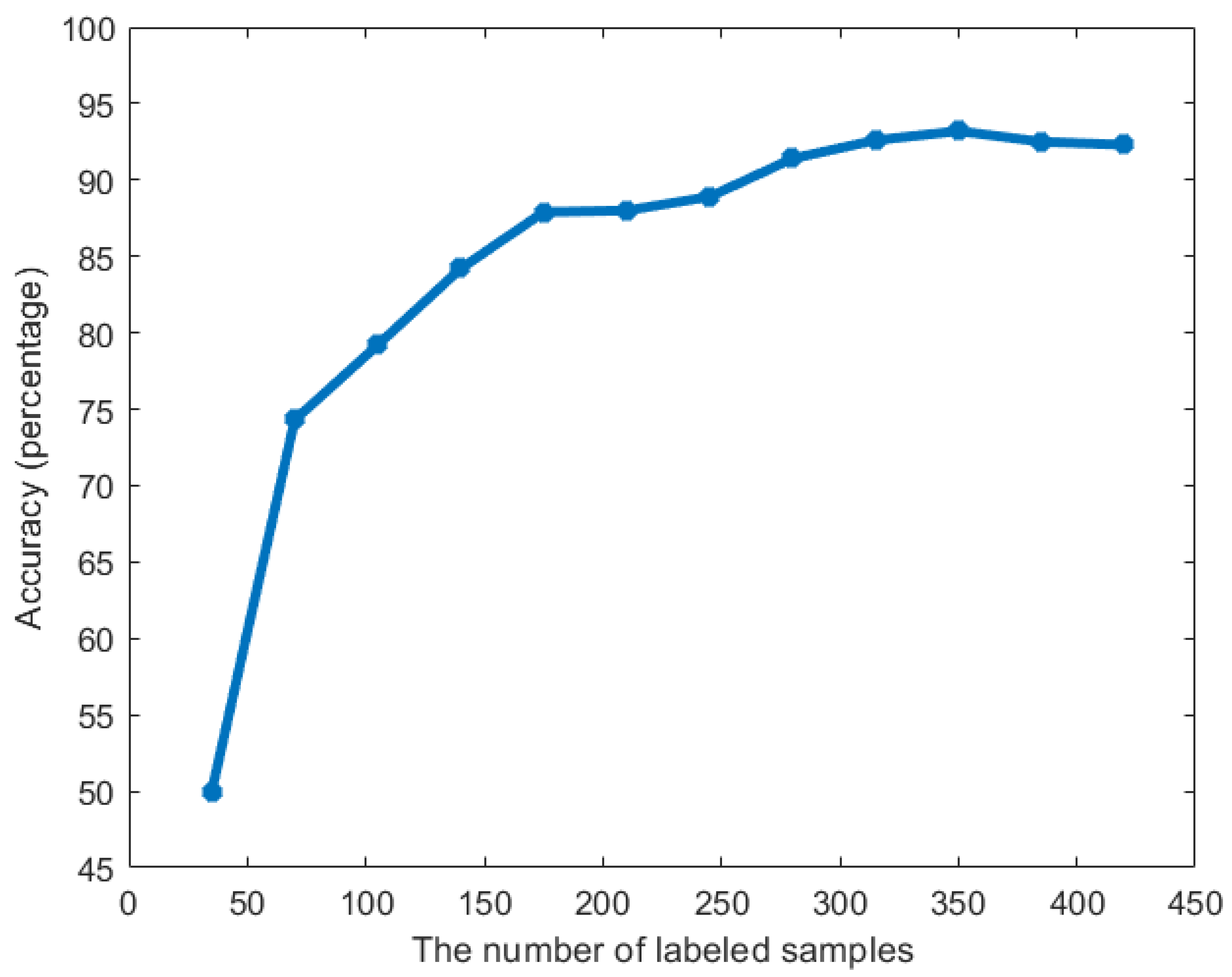
4.2.1. Accuracy Results

Table 3, Table 4, Table 5 and Table 6 show the accuracy results based on different unlabeled sets for the SVM-based methods, LDA-based methods, and KNN-based methods, where both the detection accuracies for windshear and non-windshear are shown. The average detection accuracy of each method for different feature vectors is also shown, and the bolded result in each column represents the highest average detection accuracy for the corresponding feature vector. For comparison, the numerical results of Huang’s method [16] for the same training dataset are shown in Table 7.
From these tables, we can readily find the following: (i) The windshear detection accuracies given by the optimal-transport-based schemes are higher than those of traditional supervised learning methods. (ii) The proposed scheme is robust to the optimal transport cost and size of the unlabeled dataset. (iii) The feature vector consisting of both physical properties and LiDAR velocity image texture ( f c o m ) provides the highest detection accuracy when we apply the OT (city block) + SVM method, which indicates that the features involving more windshear information can achieve superior performance with a suitable learning method. The features are linearly separable after the city block distance-based optimal transport label predetermination. (iii) Compared with the numerical results of the method proposed by Huang et al. [16], the proposed method can yield much higher windshear detection accuracy, especially when there are many windshear cases in the set of the non-reported samples.
To further illustrate the use of optimal transport, we show some details of data transportation next.

4.2.2. Data Transportation

Table 8 shows the average rounded number of unlabeled samples involved in the transport procedure during classifier training. The number of samples involved in the transportation procedure is greater than the number of pre-involved reported windshear cases (85 for this paper), especially for learning on the unlabeled datasets that involve more positive-labeled samples ( U 2 and U 4 ). This indicates that there are many windshear cases in non-reported time stamps and that the proposed optimal transport model is effective in the identification of potential windshear cases (windshear cases without pilot reports).

4.3. Windshear Prediction

Now, let us evaluate the windshear prediction performance of our proposed scheme. The prediction results for windshear in 2020 obtained by the learning classifier trained based on data obtained from 2017 to 2019 are shown. To move much closer to practical application, we apply the learning model trained based on randomly selected unlabeled cases (i.e., groups U 2 and U 4 ) to predict windshear in 2020.
Table 9 and Table 10 show the prediction accuracy results based on different groups for the SVM-based methods, LDA-based methods, and KNN-based methods, where both the detection accuracies for windshear and non-windshear are shown, and the bolded results in each column represent the highest average detection accuracy for the corresponding feature vector. For comparison, the numerical results of Huang’s method [16] for the same training dataset are shown in Table 11. There is also a noticeable improvement in the average prediction accuracy of our proposed scheme compared with those of the traditional supervised methods. Although Huang’s method can provide average accuracy comparable to that of our proposed scheme in some cases, our proposed scheme can predict windshear with accuracies greater than 90 % for most of the investigated features and learning models, which is much more important in practice. Based on these numerical results, we verify the effectiveness of our proposed methods for windshear prediction, and in the future, we can directly identify whether windshear occurs based on the pre-trained classifier, without the need to train a new classifier based on recently collected data.

5. Conclusions

In this paper, we proposed an optimal-transport-based positive and unlabeled learning scheme for windshear detection based on the fact that we do not know whether windshear occurs during non-flight time. We first predetermined the labels of the samples obtained at the non-reported timestamps by an optimal transport model and then trained a binary classifier on the predetermined information via supervised learning methods. Furthermore, since the certain timestamp of windshear occurrence cannot be ensured in practice, multiple instance learning is also used in the proposed scheme.
To evaluate the effectiveness and robustness of the proposed scheme, several numerical experiments based on the wind velocity data collected at HKIA by LiDAR PPI scan were performed in this paper. Features extracted by both the physical-properties-based method and image processing method were applied for testing. Specifically, three different distances between the investigated feature vectors were calculated for the cost matrix construction of the optimal transport model, i.e., the Euclidean distance, the squared Euclidean distance, and the city block distance. We mainly applied three supervised learning methods to train the binary classifier, including the SVM method, the LDA method, and the KNN method. For comparison, the numerical results of the method proposed by Huang et al. [16] on the same dataset were also shown in this paper. The numerical results clearly show the following: (i) The proposed optimal transport model is effective for potential windshear case recognition. (ii) The performance of the binary classifier for windshear detection and prediction can be significantly improved by the proposed OT-based PUL scheme. Moreover, this method is insensitive to the transport cost and the size of unlabeled datasets. (iii) Compared with the method proposed by Huang et al., our proposed method can detect more windshear cases. (iv) The prediction performance of our proposed scheme is quite good, indicating that one can directly predict whether windshear occurs using the pre-trained classifier, without the need to train a new classifier based on recently collected data.
In the future, we can apply the proposed scheme to detect windshear in wind velocity data collected by other means. Furthermore, we can also investigate better multiple instance learning schemes for windshear detection or better windshear feature extraction methods from the images of wind velocity data.

Author Contributions

Conceptualization, J.Z., P.-W.C. and M.K.-P.N.; Methodology, J.Z. and M.K.-P.N.; Software, J.Z.; Validation, J.Z. and P.-W.C.; Formal analysis, J.Z., P.-W.C. and M.K.-P.N.; Investigation, J.Z.; Resources, P.-W.C.; Data curation, J.Z. and P.-W.C.; Writing—original draft, J.Z.; Writing—review & editing, P.-W.C. and M.K.-P.N.; Supervision, P.-W.C. and M.K.-P.N. All authors have read and agreed to the published version of the manuscript.

Funding

This research was funded by HKRGC GRF 17300021, HKRGC CRF C7004-21GF, and Joint NSFC and RGC N-HKU769/21.

Data Availability Statement

The request for data used to support the findings of this study can be addressed to the Hong Kong Observatory. The data provision will be considered on a case-by-case basis.

Conflicts of Interest

The authors declare no conflicts of interest or competing interests.

References

  1. Chan, P.; Shun, C.; Wu, K. Operational LIDAR-based system for automatic windshear alerting at the Hong Kong International Airport. In Proceedings of the 12th Conference on Aviation, Range, and Aerospace Meteorology, Atlanta, GA, USA, 29 January–2 February 2006; Volume 6. [Google Scholar]
  2. Thobois, L.; Cariou, J.; Gultepe, I. Review of lidar-based applications for aviation weather. Pure Appl. Geophys. 2019, 176, 1959–1976. [Google Scholar] [CrossRef]
  3. ICAO. Manual on Low-Level Wind Shear; Technical Report; International Civil Aviation Organization: Montréal, QC, Canada, 2005. [Google Scholar]
  4. Weipert, A.; Kauczok, S.; Hannesen, R.; Ernsdorf, T.; Stiller, B. Wind shear detection using radar and lidar at Frankfurt and Munich airports. In Proceedings of the 8th European Conference on Radar in Meteorology and Hydrology, Garmisch-Partenkirchen, Germany, 1–5 September 2014; pp. 1–5. [Google Scholar]
  5. Li, M.; Xu, J.; Xiong, X.l.; Ma, Y.; Zhao, Y. A novel ramp method based on improved smoothing algorithm and second recognition for windshear detection using lidar. Curr. Opt. Photonics 2018, 2, 7–14. [Google Scholar]
  6. Jones, J.; Haynes, A. A Peakspotter Program Applied to the Analysis of Increments in Turbulence Velocity; Technical Report; RAE: Madrid, Spain, 1984.
  7. Woodfield, A.; Woods, J. Worldwide Experience of Wind Shear During 1981–1982; Technical Report; Royal Aircraft EstablIshment Bedford: Bedford, UK, 1983. [Google Scholar]
  8. Hon, K.; Chan, P. Improving Lidar Windshear Detection Efficiency by Removal of “Gentle Ramps”. Atmosphere 2021, 12, 1539. [Google Scholar] [CrossRef]
  9. Hinton, D.A. Airborne Derivation of Microburst Alerts from Ground-Based Terminal Doppler Weather Radar Information: A Flight Evaluation; Technical Report; National Aeronautics and Space Administration, Langley Research Center Hampton: Hampton, VA, USA, 1993.
  10. Chan, P.; Hon, K.; Shin, D. Combined use of headwind ramps and gradients based on LIDAR data in the alerting of low-level windshear/turbulence. Meteorol. Z. 2011, 20, 661. [Google Scholar] [CrossRef]
  11. Chan, P. Application of LIDAR-based F-factor in windshear alerting. Meteorol. Z. 2012, 21, 193. [Google Scholar] [CrossRef]
  12. Lee, Y.; Chan, P. LIDAR-based F-factor for wind shear alerting: Different smoothing algorithms and application to departing flights. Meteorol. Appl. 2014, 21, 86–93. [Google Scholar] [CrossRef]
  13. Wu, T.; Hon, K. Application of spectral decomposition of LIDAR-based headwind profiles in windshear detection at the Hong Kong International Airport. Meteorol. Z. 2018, 27, 33–42. [Google Scholar] [CrossRef]
  14. Li, L.; Shao, A.; Zhang, K.; Ding, N.; Chan, P. Low-Level Wind Shear Characteristics and Lidar-Based Alerting at Lanzhou Zhongchuan International Airport, China. J. Meteorol. Res. 2020, 34, 633–645. [Google Scholar] [CrossRef]
  15. Ma, Y.; Li, S.; Lu, W. Recognition of partial scanning low-level wind shear based on support vector machine. Adv. Mech. Eng. 2018, 10, 1687814017754151. [Google Scholar] [CrossRef]
  16. Huang, J.; Ng, M.; Chan, P. Wind Shear Prediction from Light Detection and Ranging Data Using Machine Learning Methods. Atmosphere 2021, 12, 644. [Google Scholar] [CrossRef]
  17. Monge, G. Mémoire sur la théorie des déblais et des remblais. In Histoire de l’Académie Royale des Sciences de Paris; Imprimerie royale: Paris, France, 1781. [Google Scholar]
  18. Kantorovitch, L. On the Translocation of Masses. Manag. Sci. 1958, 5, 1–4. [Google Scholar] [CrossRef]
  19. Cuturi, M. Sinkhorn distances: Lightspeed computation of optimal transport. Adv. Neural Inf. Process. Syst. 2013, 26, 2292–2300. [Google Scholar]
  20. Altschuler, J.; Niles-Weed, J.; Rigollet, P. Near-linear time approximation algorithms for optimal transport via Sinkhorn iteration. Adv. Neural Inf. Process. Syst. 2017, 30, 1961–1971. [Google Scholar]
  21. Dvurechensky, P.; Gasnikov, A.; Kroshnin, A. Computational optimal transport: Complexity by accelerated gradient descent is better than by Sinkhorn’s algorithm. In Proceedings of the International Conference on Machine Learning, PMLR, Stockholm, Sweden, 10–15 July 2018; pp. 1367–1376. [Google Scholar]
  22. Lin, T.; Ho, N.; Jordan, M. On the Efficiency of Entropic Regularized Algorithms for Optimal Transport. J. Mach. Learn. Res. 2022, 23, 1–42. [Google Scholar]
  23. Peyré, G.; Cuturi, M. Computational optimal transport: With applications to data science. Found. Trends® Mach. Learn. 2019, 11, 355–607. [Google Scholar] [CrossRef]
  24. Zhang, J.; Liu, T.; Tao, D. An Optimal Transport Analysis on Generalization in Deep Learning. IEEE Trans. Neural Netw. Learn. Syst. 2021, 34, 2842–2853. [Google Scholar] [CrossRef]
  25. Li, Q.; Wang, Z.; Liu, S.; Li, G.; Xu, G. Causal optimal transport for treatment effect estimation. IEEE Trans. Neural Netw. Learn. Syst. 2021, 6, 2842–2853. [Google Scholar] [CrossRef]
  26. Amores, J. Multiple instance classification: Review, taxonomy and comparative study. Artif. Intell. 2013, 201, 81–105. [Google Scholar] [CrossRef]
  27. Flamary, R.; Cuturi, M.; Courty, N.; Rakotomamonjy, A. Wasserstein discriminant analysis. Mach. Learn. 2018, 107, 1923–1945. [Google Scholar] [CrossRef]
  28. Su, B.; Zhou, J.; Wu, Y. Order-preserving wasserstein discriminant analysis. In Proceedings of the IEEE/CVF International Conference on Computer Vision, Seoul, Republic of Korea, 27 October–2 November 2019; pp. 9885–9894. [Google Scholar]
  29. Su, B.; Zhou, J.; Wen, J.; Wu, Y. Linear and Deep Order-Preserving Wasserstein Discriminant Analysis. IEEE Trans. Pattern Anal. Mach. Intell. 2021, 44, 3123–3138. [Google Scholar] [CrossRef]
  30. Arjovsky, M.; Chintala, S.; Bottou, L. Wasserstein generative adversarial networks. In Proceedings of the International Conference on Machine Learning, PMLR, Sydney, Australia, 6–11 August 2017; pp. 214–223. [Google Scholar]
  31. Tolstikhin, I.; Bousquet, O.; Gelly, S.; Schölkopf, B. Wasserstein Auto-Encoders. In Proceedings of the 6th International Conference on Learning Representations (ICLR 2018), Stockholm, Sweden, 10–15 July 2018. [Google Scholar]
  32. Courty, N.; Flamary, R.; Tuia, D.; Rakotomamonjy, A. Optimal transport for domain adaptation. IEEE Trans. Pattern Anal. Mach. Intell. 2016, 39, 1853–1865. [Google Scholar] [CrossRef] [PubMed]
  33. Courty, N.; Flamary, R.; Habrard, A.; Rakotomamonjy, A. Joint distribution optimal transportation for domain adaptation. Adv. Neural Inf. Process. Syst. 2017, 30, 3733–3742. [Google Scholar]
  34. Zhang, Z.; Wang, M.; Nehorai, A. Optimal transport in reproducing kernel hilbert spaces: Theory and applications. IEEE Trans. Pattern Anal. Mach. Intell. 2019, 42, 1741–1754. [Google Scholar] [CrossRef] [PubMed]
  35. Chapel, L.; Alaya, M.; Gasso, G. Partial optimal tranport with applications on positive-unlabeled learning. Adv. Neural Inf. Process. Syst. 2020, 33, 2903–2913. [Google Scholar]
  36. Cao, N.; Zhang, T.; Shi, X.; Jin, H. Posistive-Unlabeled Learning via Optimal Transport and Margin Distribution. In Proceedings of the Thirty-First International Joint Conference on Artificial Intelligence, IJCAI-22, Vienna, Austria, 23–29 July 2022; pp. 2836–2842. [Google Scholar]
  37. Bekker, J.; Davis, J. Learning from positive and unlabeled data: A survey. Mach. Learn. 2020, 109, 719–760. [Google Scholar] [CrossRef]
  38. Li, F.; Dong, S.; Leier, A.; Han, M.; Guo, X.; Xu, J.; Wang, X.; Pan, S.; Jia, C.; Zhang, Y.; et al. Positive-unlabeled learning in bioinformatics and computational biology: A brief review. Briefings Bioinform. 2022, 23, bbab461. [Google Scholar] [CrossRef]
  39. Zhang, Y.; Li, C.; Liu, Z.; Li, M. Semi-Supervised Disease Classification based on Limited Medical Image Data. IEEE J. Biomed. Health Inform. 2024, 28, 1575–1586. [Google Scholar] [CrossRef]
  40. Gong, C.; Shi, H.; Yang, J.; Yang, J. Multi-manifold positive and unlabeled learning for visual analysis. IEEE Trans. Circuits Syst. Video Technol. 2019, 30, 1396–1409. [Google Scholar] [CrossRef]
  41. de Souza, M.C.; Nogueira, B.M.; Rossi, R.G.; Marcacini, R.M.; Dos Santos, B.N.; Rezende, S.O. A network-based positive and unlabeled learning approach for fake news detection. Mach. Learn. 2022, 111, 3549–3592. [Google Scholar] [CrossRef]
  42. Wang, J.; Qian, S.; Hu, J.; Hong, R. Positive Unlabeled Fake News Detection Via Multi-Modal Masked Transformer Network. IEEE Trans. Multimed. 2023, 26, 234–244. [Google Scholar] [CrossRef]
  43. Li, X.; Liu, B. Learning to classify texts using positive and unlabeled data. In Proceedings of the 18th International Joint Conference on Artificial Intelligence, IJCAI-03, Acapulco, Mexico, 9–15 August 2003; pp. 587–592. [Google Scholar]
  44. Liu, B.; Dai, Y.; Li, X.; Lee, W.; Yu, P. Building text classifiers using positive and unlabeled examples. In Proceedings of the Third IEEE International Conference on Data Mining, IEEE, Melbourne, FL, USA, 19–22 November 2003; pp. 179–186. [Google Scholar]
  45. Gong, C.; Shi, H.; Liu, T.; Zhang, C.; Yang, J.; Tao, D. Loss decomposition and centroid estimation for positive and unlabeled learning. IEEE Trans. Pattern Anal. Mach. Intell. 2019, 43, 918–932. [Google Scholar] [CrossRef] [PubMed]
  46. Yang, P.; Ormerod, J.; Liu, W.; Ma, C.; Zomaya, A.; Yang, J. AdaSampling for positive-unlabeled and label noise learning with bioinformatics applications. IEEE Trans. Cybern. 2018, 49, 1932–1943. [Google Scholar] [CrossRef] [PubMed]
  47. Gu, W.; Zhang, T.; Jin, H. Entropy Weight Allocation: Positive-unlabeled Learning via Optimal Transport. In Proceedings of the 2022 SIAM International Conference on Data Mining (SDM), SIAM, Alexandria, VA, USA, 28–30 April 2022; pp. 37–45. [Google Scholar]
  48. Zhang, J.; Chan, P.; Ng, M. LiDAR-Based Windshear Detection via Statistical Features. Adv. Meteorol. 2022, 2022. [Google Scholar] [CrossRef]
  49. Xu, H. Convergence analysis of the Frank-Wolfe algorithm and its generalization in Banach spaces. arXiv 2017, arXiv:1710.07367. [Google Scholar]
Figure 1. The locations of the Doppler LiDARs at HKIA (indicated by blue spades).
Remotesensing 16 04423 g001
Figure 2. An example of the LiDAR observational wind velocity data (knots) collected on 7 February 2017 at HKIA.
Remotesensing 16 04423 g002
Figure 3. The algorithmic chart of the proposed scheme.
Remotesensing 16 04423 g003
Figure 4. The curve of testing accuracy for different numbers of labeled samples with fixed parameter γ = 1 .
Remotesensing 16 04423 g004
Table 1. Description of the unlabeled datasets used for numerical experiments.
Dataset NameDataset SizeDescription
U 1 535Non-reported cases collected at the most likely non-windshear timestamps.
U 2 535Non-reported cases collected at randomly selected timestamps.
U 3 731Non-reported cases collected at the most likely non-windshear timestamps.
U 4 719Non-reported cases collected at randomly selected timestamps.
Table 2. Percentage of correctly identified pre-involved reported windshear cases according to Equation (13) for the construction of different cost matrices with fixed model parameter γ = 1 .
Cost Matrix Construction f p f im f com f h
Euclidean distance 92.24 % 90.59 % 90.24 % 80.82 %
Squared Euclidean distance 95.53 % 95.53 % 89.88 % 81.00 %
City block distance 91.53 % 92.94 % 93.41 % 81.00 %
Table 3. Detection accuracy of different methods for different feature vectors on the training dataset with unlabeled set U 1 .
MethodsAccuracy f p f im f com f h
SVMWindshear detection 93.20 % 83.20 % 94.40 % 80.40 %
Non-windshear detection 92.80 % 92.20 % 93.60 % 92.40 %
Average 93.00 % 87.70 % 94.00 % 86.40 %
OT (Euclidean) + SVMWindshear detection 91.00 % 88.80 % 96.50 % 88.00 %
Non-windshear detection 95.50 % 88.80 % 91.75 % 86.25 %
Average 93.25 % 88.80 % 94.13 % 87 . 13 %
OT (squared Euclidean) + SVMWindshear detection 95.60 % 90.40 % 96.50 % 85.20 %
Non-windshear detection 90.60 % 87.60 % 91.75 % 88.00 %
Average 93.10 % 89.00 % 94.13 % 86.60 %
OT (city block) + SVMWindshear detection 95.80 % 88.60 % 98.00 % 88.25 %
Non-windshear detection 90.60 % 88.60 % 90.50 % 86.00 %
Average 93.20 % 89.20 % 94 . 25 % 87 . 13 %
LDAWindshear detection 82.20 % 83.80 % 86.40 % 78.40 %
Non-windshear detection 96.80 % 93.2 % 95.80 % 93.80 %
Average 89.50 % 88.50 % 91.10 % 86.10 %
OT (Euclidean) + LDAWindshear detection 96.40 % 85.00 % 89.00 % 83.80 %
Non-windshear detection 89.80 % 93.00 % 93.80 % 89.60 %
Average 93.10 % 89.00 % 91.40 % 86.70 %
OT (squared Euclidean) + LDAWindshear detection 94.60 % 85.00 % 89.60 % 82.80 %
Non-windshear detection 91.80 % 93.00 % 93.20 % 89.80 %
Average 93.20 % 89.00 % 91.40 % 86.30 %
OT (city block) + LDAWindshear detection 95.40 % 86.00 % 91.40 % 83.20 %
Non-windshear detection 91.00 % 93.00 % 92.60 % 89.80 %
Average 93.20 % 89.50 % 92.00 % 86.50 %
KNNWindshear detection 94.40 % 88.60 % 92.20 % 81.00 %
Non-windshear detection 92.60 % 89.20 % 92.60 % 92.00 %
Average 93.50 % 88.90 % 92.40 % 86.50 %
OT (Euclidean) + KNNWindshear detection 95.40 % 92.60 % 97.40 % 87.00 %
Non-windshear detection 91.80 % 86.80 % 87.80 % 87.00 %
Average 93.60 % 89 . 70 % 92.60 % 87.00 %
OT (squared Euclidean) + KNNWindshear detection 95.20 % 92.60 % 97.25 % 85.20 %
Non-windshear detection 92.40 % 85.40 % 88.25 % 88.00 %
Average 93 . 80 % 89.00 % 92.75 % 86.60 %
OT (city block) + KNNWindshear detection 95.20 % 92.60 % 97.75 % 87.75 %
Non-windshear detection 92.20 % 85.40 % 87.25 % 86.25 %
Average 93.70 % 89.00 % 92.50 % 87.00 %
Table 4. Detection accuracy of different methods for different feature vectors on the training dataset with unlabeled set U 2 .
MethodsAccuracy f p f im f com f h
SVMWindshear detection 77.00 % 77.00 % 76.00 % 74.60 %
Non-windshear detection 98.20 % 95.00 % 98.80 % 96.80 %
Average 87.60 % 86.00 % 87.40 % 85.70 %
OT (Euclidean) + SVMWindshear detection 92.60 % 88.40 % 94.60 % 83.60 %
Non-windshear detection 94.00 % 90.60 % 92.60 % 89.60 %
Average 93.30 % 89.50 % 93 . 60 % 86.60 %
OT (squared Euclidean) + SVMWindshear detection 94.60 % 87.80 % 93.20 % 79.40 %
Non-windshear detection 92.00 % 89.80 % 93.00 % 92.40 %
Average 93.30 % 88.80 % 93.10 % 85.90 %
OT (city block) + SVMWindshear detection 93.20 % 88.40 % 94.00 % 80.60 %
Non-windshear detection 93.40 % 91.20 % 92.20 % 93.00 %
Average 93.30 % 89 . 80 % 93.10 % 86 . 80 %
LDAWindshear detection 74.60 % 75.00 % 75.20 % 73.40 %
Non-windshear detection 99.20 % 95.00 % 97.40 % 97.00 %
Average 86.90 % 85.00 % 86.30 % 85.20 %
OT (Euclidean) + LDAWindshear detection 91.20 % 88.20 % 93.20 % 79.40 %
Non-windshear detection 94.20 % 91.20 % 85.80 % 93.00 %
Average 92.70 % 89.70 % 89.50 % 86.20 %
OT (squared Euclidean) + LDAWindshear detection 95.40 % 87.60 % 87.40 % 82.20 %
Non-windshear detection 89.60 % 91.20 % 92.80 % 90.60 %
Average 92.50 % 89.40 % 90.10 % 86.40 %
OT (city block) + LDAWindshear detection89.40%86.40%89.60%79.40%
Non-windshear detection 95.20 % 91.60 % 94.00 % 93.00 %
Average 92.30 % 89.00 % 91.80 % 86.20 %
KNNWindshear detection 87.00 % 81.60 % 82.20 % 74.20 %
Non-windshear detection 95.40 % 91.40 % 96.00 % 96.60 %
Average 91.20 % 86.50 % 89.10 % 85.40 %
OT (Euclidean) + KNNWindshear detection 95.20 % 88.80 % 90.80 % 77.80 %
Non-windshear detection 91.40 % 89.20 % 90.20 % 93.80 %
Average 93.30 % 89.00 % 90.50 % 85.80 %
OT (squared Euclidean) + KNNWindshear detection 95.00 % 88.00 % 89.60 % 80.80 %
Non-windshear detection 91.80 % 91.40 % 89.40 % 92.00 %
Average 93.40 % 89.70 % 89.50 % 86.40 %
OT (city block) + KNNWindshear detection 93.40 % 87.20 % 92.80 % 79.20 %
Non-windshear detection 93.60 % 91.20 % 91.00 % 94.20 %
Average 93 . 50 % 89.20 % 91.90 % 86.70 %
Table 5. Detection accuracy of different methods for different feature vectors on the training dataset with unlabeled set U 3 .
MethodsAccuracy f p f im f com f h
SVMWindshear detection 91.80 % 78.40 % 91.60 % 79.40 %
Non-windshear detection 96.40 % 93.80 % 95.60 % 94.40 %
Average 94.10 % 86.10 % 93.60 % 86.90 %
OT (Euclidean) + SVMWindshear detection 95.00 % 88.40 % 96.20 % 85.20 %
Non-windshear detection 94.40 % 90.20 % 92.40 % 90.60 %
Average 94.70 % 89.30 % 94.30 % 87.90 %
OT (squared Euclidean) + SVMWindshear detection 95.40 % 89.20 % 97.40 % 84.80 %
Non-windshear detection 94.40 % 91.80 % 91.20 % 90.80 %
Average 94.90 % 90 . 50 % 94.30 % 87.80 %
OT (city block) + SVMWindshear detection 95.60 % 88.40 % 96.00 % 85.20 %
Non-windshear detection 94.40 % 91.20 % 94.80 % 90.60 %
Average 95.00 % 89.80 % 95 . 40 % 87.90 %
LDAWindshear detection 81.60 % 79.00 % 86.00 % 77.80 %
Non-windshear detection 98.60 % 95.40 % 97.80 % 97.60 %
Average 90.10 % 87.20 % 91.90 % 87.70 %
OT (Euclidean) + LDAWindshear detection 95.20 % 84.80 % 90.40 % 82.20 %
Non-windshear detection 95.20 % 93.60 % 96.20 % 93.60 %
Average 95 . 20 % 89.20 % 93.30 % 87.90 %
OT (squared Euclidean) + LDAWindshear detection 94.60 % 84.80 % 89.40 % 82.20 %
Non-windshear detection 95.20 % 93.60 % 96.60 % 94.00 %
Average 94.90 % 89.20 % 93.00 % 88.10 %
OT (city block) + LDAWindshear detection 91.80 % 85.80 % 89.20 % 81.60 %
Non-windshear detection 96.20 % 92.80 % 96.80 % 94.40 %
Average 94.00 % 89.30 % 93.00 % 88.00 %
KNNWindshear detection 90.60 % 89.60 % 93.20 % 78.40 %
Non-windshear detection 96.00 % 91.00 % 94.40 % 96.80 %
Average 93.30 % 90.30 % 93.80 % 87.60 %
OT (Euclidean) + KNNWindshear detection 95.60 % 93.60 % 94.00 % 85.40 %
Non-windshear detection 94.40 % 87.20 % 91.00 % 91.00 %
Average 95.00 % 90.40 % 92.50 % 88.20 %
OT (squared Euclidean) + KNNWindshear detection 95.80 % 93.60 % 94.40 % 85.40 %
Non-windshear detection 94.40 % 87.40 % 91.80 % 91.00 %
Average 95.10 % 90 . 50 % 93.10 % 88.20 %
OT (city block) + KNNWindshear detection 95.80 % 94.60 % 96.20 % 85.20 %
Non-windshear detection 94.20 % 85.80 % 89.60 % 91.60 %
Average 95.00 % 90.20 % 92.90 % 88 . 40 %
Table 6. Detection accuracy of different methods for different feature vectors on the training dataset with unlabeled set U 4 .
MethodsAccuracy f p f im f com f h
SVMWindshear detection 71.20 % 73.00 % 72.00 % 66.60 %
Non-windshear detection 100.00 % 95.60 % 99.40 % 99.60 %
Average 85.60 % 84.30 % 85.70 % 83.10 %
OT (Euclidean) + SVMWindshear detection 90.40 % 85.40 % 91.20 % 79.40 %
Non-windshear detection 97.80 % 93.60 % 96.40 % 96.20 %
Average 94.10 % 89.50 % 93.80 % 87.80 %
OT (squared Euclidean) + SVMWindshear detection 92.60 % 90.20 % 89.40 % 80.20 %
Non-windshear detection 96.20 % 89.20 % 97.60 % 95.80 %
Average 94.40 % 89.70 % 93.50 % 88.00 %
OT (city block) + SVMWindshear detection 92.60 % 83.60 % 92.20 % 80.40 %
Non-windshear detection 96.60 % 95.20 % 96.60 % 95.80 %
Average 94.60 % 89.40 % 94 . 40 % 88 . 10 %
LDAWindshear detection 71.00 % 73.20 % 70.60 % 66.40 %
Non-windshear detection 99.80 % 95.60 % 99.20 % 99.80 %
Average 85.40 % 84.40 % 84.90 % 83.10 %
OT (Euclidean) + LDAWindshear detection 92.00 % 87.80 % 91.20 % 80.00 %
Non-windshear detection 96.40 % 92.60 % 90.60 % 95.80 %
Average 94.20 % 90 . 20 % 90.90 % 87.90 %
OT (squared Euclidean) + LDAWindshear detection 97.00 % 89.80 % 86.80 % 82.00 %
Non-windshear detection 93.00 % 90.40 % 94.80 % 94.20 %
Average 95.00 % 90.10 % 90.80 % 88.10 %
OT (city block) + LDAWindshear detection 88.60 % 85.20 % 87.20 % 79.00 %
Non-windshear detection 97.40 % 93.40 % 97.00 % 96.60 %
Average 93.00 % 89.30 % 92.10 % 87.80 %
KNNWindshear detection 71.20 % 73.40 % 77.00 % 66.40 %
Non-windshear detection 99.40 % 95.40 % 97.00 % 99.80 %
Average 85.30 % 84.40 % 87.00 % 83.10 %
OT (Euclidean) + KNNWindshear detection 94.80 % 90.00 % 88.80 % 77.20 %
Non-windshear detection 95.00 % 89.40 % 89.40 % 97.80 %
Average 94.90 % 89.70 % 89.10 % 87.50 %
OT (squared Euclidean) + KNNWindshear detection 96.80 % 85.80 % 92.60 % 79.80 %
Non-windshear detection 93.80 % 93.40 % 84.60 % 96.20 %
Average 95 . 30 % 89.60 % 88.60 % 88.00 %
OT (city block) + KNNWindshear detection 92.60 % 87.40 % 92.60 % 78.40 %
Non-windshear detection 96.00 % 91.40 % 91.40 % 96.20 %
Average 94.30 % 89.40 % 92.00 % 87.30 %
Table 7. Numerical results of the method proposed by Huang et al. [16].
GroupResultWindshearNon-WindshearAccuracy
U 1 Ground Truth Windshear8614 86.50 %
Ground Truth
Non-Windshear
1387
U 2 Ground Truth Windshear7525 85.50 %
Ground Truth
Non-Windshear
496
U 3 Ground Truth Windshear8614 87.50 %
Ground Truth
Non-Windshear
1189
U 4 Ground Truth Windshear7525 86.50 %
Ground Truth
Non-Windshear
298
Table 8. Average rounded number of transported samples for different cost matrix constructions during the training procedure.
GroupCost Matrix Construction f p f im f com f h
U 1 Euclidean distance132130125113
Squared Euclidean distance133131123110
City Block Distance133136124112
U 2 Euclidean distance202186177175
Squared Euclidean distance223184166181
City Block Distance187178179168
U 3 Euclidean distance158150151153
Squared Euclidean distance139149145137
City Block Distance150170138142
U 4 Euclidean distance239242234201
Squared Euclidean distance223245233232
City Block Distance223207221200
Table 9. Prediction accuracy of windshear and non-windshear cases in 2020 by the classifiers trained on U 2 .
MethodsAccuracy f p f im f com f h
SVMWindshear detection 87.00 % 84.40 % 85.40 % 84.00 %
Non-windshear detection 92.20 % 85.00 % 91.60 % 96.00 %
Average 89.60 % 84.70 % 88.50 % 90.00 %
OT (Euclidean) + SVMWindshear detection 95.40 % 92.20 % 95.20 % 89.60 %
Non-windshear detection 91.00 % 83.40 % 89.00 % 90.60 %
Average 93.20 % 87.80 % 92.10 % 90.10 %
OT (squared Euclidean) + SVMWindshear detection 97.80 % 92.20 % 94.60 % 89.80 %
Non-windshear detection 89.40 % 83.20 % 89.60 % 90.60 %
Average 93.60 % 87.70 % 92.10 % 90 . 20 %
OT (city block) + SVMWindshear detection 95.80 % 92.00 % 96.00 % 89.60 %
Non-windshear detection 91.20 % 82.40 % 90.00 % 90.60 %
Average 93.50 % 87.20 % 93 . 00 % 90.10 %
LDAWindshear detection 83.80 % 80.40 % 84.40 % 83.80 %
Non-windshear detection 92.20 % 86.00 % 91.20 % 96.00 %
Average 88.00 % 83.20 % 87.80 % 89.90 %
OT (Euclidean) + LDAWindshear detection 95.80 % 91.80 % 90.80 % 89.25 %
Non-windshear detection 90.80 % 83.00 % 90.20 % 90.75 %
Average 93.30 % 87.40 % 90.50 % 90.00 %
OT (squared Euclidean) + LDAWindshear detection 97.40 % 92.20 % 90.80 % 89.40 %
Non-windshear detection 90.00 % 81.40 % 89.40 % 90.60 %
Average 93 . 70 % 86.80 % 90.10 % 90.00 %
OT (city block) + LDAWindshear detection 94.80 % 90.20 % 92.80 % 89.25 %
Non-windshear detection 91.80 % 83.60 % 90.00 % 90.75 %
Average 93.30 % 86.90 % 91.40 % 90.00 %
KNNWindshear detection 91.40 % 80.40 % 87.80 % 83.60 %
Non-windshear detection 92.00 % 85.20 % 88.60 % 95.80 %
Average 91.70 % 82.80 % 88.20 % 89.70 %
OT (Euclidean) + KNNWindshear detection 96.80 % 91.80 % 95.00 % 90.00 %
Non-windshear detection 90.00 % 82.80 % 81.75 % 89.60 %
Average 93.40 % 87.30 % 88.38 % 89.80 %
OT (squared Euclidean) + KNNWindshear detection 96.00 % 92.80 % 93.75 % 90.00 %
Non-windshear detection 91.40 % 83.00 % 84.50 % 90.00 %
Average 93 . 70 % 87 . 90 % 89.13 % 90.00 %
OT (city block) + KNNWindshear detection 95.80 % 93.00 % 94.00 % 86.20 %
Non-windshear detection 91.20 % 82.40 % 83.20 % 93.40 %
Average 93.50 % 87.70 % 88.60 % 89.80 %
Table 10. Prediction accuracy of windshear and non-windshear cases in 2020 by the classifiers trained on U 4 .
MethodsAccuracy f p f im f com f h
SVMWindshear detection 79.00 % 77.40 % 79.60 % 81.00 %
Non-windshear detection 93.80 % 87.20 % 93.20 % 96.00 %
Average 86.40 % 82.30 % 86.40 % 88.50 %
OT (Euclidean) + SVMWindshear detection 95.60 % 92.00 % 93.80 % 86.40 %
Non-windshear detection 91.60 % 83.60 % 90.40 % 94.20 %
Average 93.60 % 87.80 % 92.10 % 90.30 %
OT (squared Euclidean) + SVMWindshear detection 96.00 % 92.00 % 95.20 % 86.20 %
Non-windshear detection 91.80 % 83.40 % 89.00 % 94.80 %
Average 93.90 % 87.70 % 92.10 % 90 . 50 %
OT (city block) + SVMWindshear detection 95.80 % 91.00 % 95.80 % 86.80 %
Non-windshear detection 91.20 % 84.60 % 90.40 % 93.60 %
Average 93.50 % 87.80 % 93 . 10 % 90.20 %
LDAWindshear detection 77.00 % 77.00 % 81.20 % 80.40 %
Non-windshear detection 93.60 % 87.60 % 92.80 % 96.00 %
Average 85.30 % 82.30 % 87.00 % 88.20 %
OT (Euclidean) + LDAWindshear detection 94.60 % 91.60 % 90.20 % 88.00 %
Non-windshear detection 91.80 % 83.80 % 91.60 % 92.40 %
Average 93.20 % 87.70 % 90.90 % 90.20 %
OT (squared Euclidean) + LDAWindshear detection 98.40 % 91.40 % 89.80 % 87.00 %
Non-windshear detection 89.80 % 83.80 % 91.60 % 93.60 %
Average 94 . 10 % 87.60 % 90.70 % 90.30 %
OT (city block) + LDAWindshear detection 93.80 % 89.40 % 92.20 % 88.80 %
Non-windshear detection 91.80 % 84.00 % 90.20 % 90.80 %
Average 92.80 % 86.70 % 91.20 % 89.80 %
KNNWindshear detection 80.00 % 79.80 % 81.20 % 79.40 %
Non-windshear detection 93.60 % 88.40 % 90.20 % 96.80 %
Average 86.80 % 84.10 % 85.70 % 88.10 %
OT (Euclidean) + KNNWindshear detection 96.40 % 91.80 % 91.00 % 89.40 %
Non-windshear detection 91.00 % 84.00 % 81.60 % 90.00 %
Average 93.70 % 87 . 90 % 86.30 % 89.70 %
OT (squared Euclidean) + KNNWindshear detection 95.80 % 91.80 % 91.60 % 90.40 %
Non-windshear detection 91.40 % 83.80 % 82.60 % 90.00 %
Average 93.60 % 87.80 % 87.10 % 90.20 %
OT (city block) + KNNWindshear detection 95.80 % 92.20 % 94.00 % 85.40 %
Non-windshear detection 91.40 % 83.60 % 85.20 % 94.20 %
Average 93.60 % 87 . 90 % 89.60 % 89.80 %
Table 11. Prediction accuracy of windshear and non-windshear cases in 2020 by the learning model proposed by Huang et al. [16] based on data collected from 2017 to 2019.
GroupResultWindshearNon-WindshearAccuracy
U 2 Ground Truth Windshear8317 89.50 %
Ground Truth
Non-Windshear
496
U 4 Ground Truth Windshear8217 89.00 %
Ground Truth
Non-Windshear
496
Disclaimer/Publisher’s Note: The statements, opinions and data contained in all publications are solely those of the individual author(s) and contributor(s) and not of MDPI and/or the editor(s). MDPI and/or the editor(s) disclaim responsibility for any injury to people or property resulting from any ideas, methods, instructions or products referred to in the content.

