Root-Zone Salinity in Irrigated Arid Farmland: Revealing Driving Mechanisms of Dynamic Changes in China’s Manas River Basin over 20 Years

Abstract

The risk of soil salinization is prevalent in arid and semi-arid regions, posing a critical challenge to sustainable agriculture. This study addresses the need for accurate assessment of regional root-zone soil salt content (SSC) and understanding of underlying driving mechanisms, which are essential for developing effective salinization mitigation and water management strategies. A remote sensing inversion technique, initially proposed to estimate root-zone SSC in cotton fields, was adapted and validated more widely to non-cotton farmlands. Validation results (with a coefficient of determination R² > 0.53) were obtained using data from a three-year (2020–2022) regional survey conducted in the arid Manas River Basin (MRB), Xinjiang, China. Based on this adapted technique, we analyzed the spatiotemporal distributions of root-zone SSC across all farmlands in MRB from 2001 to 2022. Findings showed that root-zone SSC decreased significantly from 5.47 to 3.77 g kg⁻¹ over the past 20 years but experienced a slight increase of 0.15 g kg⁻¹ in recent five years (2017–2022), attributed to cultivated area expansion and reduced irrigation quotas due to local water shortages. The driving mechanisms behind root-zone SSC distributions were analyzed using an approach combined with two machine learning algorithms, eXtreme Gradient Boosting (XGBoost) and SHapley Additive exPlanation (SHAP), to identify influential factors and quantify their impacts. The approach demonstrated high predictive accuracy (R² = 0.96 ± 0.01, root mean squared error RMSE = 0.19 ± 0.03 g kg⁻¹, maximum absolute error MAE = 0.14 ± 0.02 g kg⁻¹) in evaluating SSC drivers. Factors such as initial SSC, crop type distribution, duration of film mulched drip irrigation implementation, normalized difference vegetation index (NDVI), irrigation amount, and actual evapotranspiration (ET_a), with mean ($\left|\mathrm{SHAP} \mathrm{value}\right|$) ≥ 0.02 g kg⁻¹, were found to be more closely correlated with root-zone SSC variations than other factors. Decreased irrigation amount appeared as the primary driver for recent increased root-zone SSC, especially in the mid- and down-stream sections of MRB. Recommendations for secondary soil salinization risk reduction include regulation of the planting structure (crop choice and extent of planting area) and maintenance of a sufficient irrigation amount.

1. Introduction

Soil salinization, a major ecological and environmental problem frequently encountered in arid and semi-arid areas, significantly affects crop growth and yield, and thus agricultural sustainable development [1]. Approximately 20% of the world’s cultivated land is impacted by soil salinity, and this is expected to expand as a function of climate change and unsustainable land management [2]. Water scarcity, another unavoidable challenge in arid and semi-arid areas, has promoted adoption of various water-saving irrigation technologies. In arid Xinjiang, China, where irrigation quotas to farmers are low, this includes the use of film mulched drip irrigation (FMDI) technology, allowing high irrigation frequency and potentially significant conservation of water [3,4]. However, agronomic management under FMDI is challenged, mainly due to the tendency of salts to be leached from the upper to lower root-zone and increase the risk of secondary salinization [5]. Accurately understanding the salinization status and dynamics of cropping soils is of significant practical importance for advancing regional agricultural production and ensuring sustainable development of water-saving irrigation practices in arid and semi-arid farmland. Furthermore, dynamics of root-zone soil salt content (SSC) are a function of numerous complex factors, including crop, topography, soil, hydrology, climate, and human activity [6]. Unraveling the driving mechanisms behind the dynamics of soil salinity should be useful for devising appropriate and efficient management strategies to mitigate adverse effects on crops and ecosystems.

Remote sensing, particularly due to its capacity to rapidly survey vast areas, has emerged as a pivotal tool for cost-effective monitoring of regional soil salinization [7]. Given that current remote sensing techniques such as optical and microwave methods primarily capture surface data [8], previous studies have predominantly concentrated on surface soil layers, with less attention given to the distribution patterns of salinity within the entire root-zone (especially the lower root-zone) [9,10]. In view of the advances of remote sensing technology for retrieving crop evapotranspiration (ET), models such as the surface energy balance system (SEBS) and the enhanced spatial and temporal adaptive reflection fusion model (ESTARFM) have been successfully applied in estimating both regional actual and relative ET [11]. Such estimations of ET inherently encompass information concerning soil water and salt stress-causing factors. Consequently, on the premise of isolating the effect of salinity from that of water stress, the root-zone SSC can feasibly be assessed using the correlation between relative ET and the soil salt stress correction coefficient [12]. Such an approach was proven to be effective in analyzing the spatiotemporal distributions of root-zone SSC of cotton fields under FMDI from 2000 to 2020 in the Manas River Basin (MRB) of Xinjiang, an arid region in northwest China [12]. The applicability of the approach for agricultural landscape beyond cotton fields, which in MRB includes a variety of other crops such as maize, wheat, and vegetables, has yet to be evaluated.

The driving factors of root-zone SSC are often analyzed using linear statistical methods such as Pearson correlation and Generalized Least Squares (GLS) [13,14]. While these methods are simple, interpretable, and computationally efficient, they are limited by a few unreasonable assumptions such as linear relationships between SSC and various influencing factors, which may not hold under actual field conditions. Many other statistical models, such as generalized additive models and kernel methods, are often employed to handle various non-linear relationships. However, they still exhibit a few drawbacks, like the need for manual specification of interaction terms or kernel functions, which extremely restricts their application in complex data structures and their ability to explain and quantify interaction effects [15,16]. Alternatively, machine learning algorithms, such as support vector machine (SVM), random forest (RF), and eXtreme Gradient Boosting (XGBoost) excel at capturing complex, non-linear interactions among variables, thus leading to improved identification of driving factors and more accurate regression results [17]. Moreover, the efficient nature of machine learning operations makes them well-suited for handling spatiotemporal big data. Consequently, there has been a growing utilization of machine-learning algorithms for SSC regression prediction in recent years [18,19,20]. However, such black-box models are challenged to effectively explain the mechanisms or analyze the magnitude of various influencing factors on SSC variability. SHapley Additive exPlanation (SHAP) is a method to enhance the interpretability of machine learning models [21]. It precisely quantifies each variable’s individual contribution as well as the interaction effects between variables, providing rich visualization tools that enable researchers to more intuitively understand the influence of each factor, thereby enhancing the model’s interpretability and transparency. The method is grounded in the principle of Shapley values from cooperative game theory, which allocates the contribution of different factors to the prediction outcome, thus promoting understanding of the driving mechanisms of each influencing factor on the model’s predictive results [22]. Theoretically, SHAP can be used to explain all the outputs of any machine-learning model. However, TreeSHAP, an improved SHAP algorithm developed specifically for tree-based models, demonstrates more efficient and precise explanatory properties [23]. XGBoost is a widely popular tree-based machine-learning model with high accuracy and efficiency [24], shown to be relevant in soil-related studies [25,26,27]. For instance, XGBoost was integrated with the SHAP algorithm to predict surface SSC and elucidate the roles of different influencing factors [28].

This study focused on root-zone SSC in cultivated farmlands (including cotton and non-cotton fields) of MRB, where sustainable agricultural practices are seriously threatened by secondary salinization risks. A remote sensing inversion method that previously succeeded in estimating root-zone SSC in cotton fields under FMDI [12] was applied more widely to non-cotton fields. Two advanced machine learning algorithms, XGBoost and TreeSHAP, were combined to facilitate in-depth interpretation of factor interactions and their contributions in root-zone SSC variations. Therefore, the objectives of this study were: (1) to establish and validate the remote sensing inversion model for estimating root-zone SSC in non-cotton fields and subsequently analyze the spatiotemporal evolution of root-zone SSC for all farmlands, including cotton and non-cotton fields within the basin from 2001 to 2022; (2) to reveal the driving mechanisms behind root-zone SSC changes over the past two decades by integrating XGBoost and TreeSHAP algorithms; and (3) to propose scientifically based regulatory measures for prevention and control of secondary soil salinization, which should be beneficial for the sustainable management of agricultural water and soil resources in arid regions.

2. Materials and Methods

2.1. Overview of Study Area

The MRB, located at the southern edge of the Junggar Basin and northern foothills of the Tianshan Mountains (Figure 1) in China, encompasses an oasis irrigation zone of about 1.1 × 10⁴ km² (43°50′–45°18′N, 84°46′–86°32′E). Characterized by a temperate continental climate, it has an average annual precipitation of 177.5 mm and potential evaporation of 1547 mm, with altitude ranging from 5242 to 256 m. A rich variety of natural soil types, primarily including anthropogenic, sandy, and saline, are distributed in the study area. The basin is divided into upstream, midstream, and downstream regions based on natural surroundings and hydrological conditions, further divided into mountain, piedmont plain, oasis plain, and oasis–desert transition zone—based on topography and research purposes (Figure 1) [29]. The mountain and piedmont plain areas are classified as upstream, the oasis plain is midstream, and the oasis–desert transition zone is downstream. At the edge of alluvial fans in the oasis plain lies a narrow spring overflow belt, where lakes, depressions, and reservoirs are concentrated. Significant geographic, vegetation, soil texture, and groundwater differences exist among the four areas. Generally, soil texture becomes finer downstream, while groundwater is shallowest at the spring overflow zone and deepens with distance. Groundwater and soil salinity are highest in this zone [30]. The hydrological system comprises the Manas, Ningjia, Jingou, and Bayingou rivers. Since the 1950s, irrigated agriculture has established ten major oasis irrigation zones, mainly in mid- and downstream areas favorable for cropping. However, flood irrigation has caused secondary soil salinization in these regions. Since the late 20th century, FMDI technology has facilitated crop cultivation on salinized soils [31]. Currently, the basin utilizes water-saving irrigation and agricultural mechanization. Planting structures vary: upstream primarily grows maize and wheat, while mid- and downstream areas focus on cotton due to improved conditions. In 2022, remote sensing identified cotton covering about 4472 km², or 86% of the cropped area, with wheat and maize accounting for 98% of the remainder [32]. Other crops, such as grapes and peppers, are also present.

2.2. Inversion and Data Collection of Root-Zone SSC

2.2.1. Remote Sensing Inversion Method of Root-Zone SSC

In order to expand the work of Yang et al. [12] for cotton, the remote sensing inversion method was used to estimate root-zone SSC of non-cotton fields in the basin. Parameters related to salt tolerance characteristics, including salt tolerance thresholds and the shape index of salinity stress response functions, were renewed or fitted accordingly. The dominant non-cotton crops, maize and wheat, have unique local growth periods and irrigation methods. Wheat mainly grows under non-mulched drip irrigation between March and August, while maize is usually cultivated under FMDI with a growing period from April to October, similar to cotton. Minor crops such as pepper and grape share growing periods and watering techniques similar to those of maize. Therefore, non-cotton crops were classified into two categories: wheat and maize, with the minor crops included as maize, and SSC inversion was thereby carried out according to three categories: cotton, wheat, and maize.

The root-zone SSC inversion method proposed by Yang et al. [12] is based on soil-crop water relations in the salinized farmland, where the degree of crop water deficit is approximated by soil water and salinity stress response functions:

$$1-{\displaystyle \frac{T_a}{T_p}}\approx 1-\gamma \left(\overline{h}\right)\beta \left(\overline{\phi }\right),$$

(1)

$$\beta \left(\overline{\phi }\right)=\left\{\begin{array}{cc}1& 0\le \overline{\phi }\le {\phi }_L\\ 1-{\left({\displaystyle \frac{\overline{\phi }-{\phi }_L}{{\phi }_W-{\phi }_L}}\right)}^{\tau }& {\phi }_L<\overline{\phi }<{\phi }_w\\ 0& \overline{\phi }\ge {\phi }_w\end{array}\right.,$$

(2)

where T_a and T_p are the actual and potential transpiration rates (mm d⁻¹), respectively; $\gamma \left(\overline{h}\right)$ and $\beta \left(\overline{\phi }\right)$ are the soil water and salinity stress response functions, respectively, in which $\overline{h}$ (cm) and $\overline{\phi }$ (g kg⁻¹) are the mean root-zone averaged soil matric potential and SSC; τ is a fitting parameter; and φ_L and φ_w are the critical and limit salinity of crop salt tolerance (g kg⁻¹), respectively. In the inversion method, two assumptions were utilized for the peak growth stage of the crop: (1) the relative transpiration (T_a/T_p) is approximated as relative evapotranspiration (ET_a/ET_p); and (2) $\gamma \left(\overline{h}\right)$ is linearly proportional to the ratio of relative water supply, viz:

$${\displaystyle \frac{T_a}{T_p}}\approx {\displaystyle \frac{E{T}_a}{E{T}_p}},$$

(3)

$$\gamma \left(\overline{h}\right)\approx \alpha \times {\displaystyle \frac{I+P}{E{T}_p\times \Delta t}},$$

(4)

where ET_a and ET_p are respectively the actual and potential evapotranspiration (ET) rate (mm d⁻¹); I and P are the irrigation amount and effective precipitation (mm) in a period of Δt (d); and α is a proportionality factor. Subsequently, with distributions of ET_a through inversely determined remote sensing fusion, the average root-zone SSC-$\overline{\phi }$ was estimated by combining Equations (1)–(4):

$$\overline{\phi }\approx \left\{\begin{array}{c}\begin{array}{cc}\begin{array}{llllll}\begin{array}{cc}\begin{array}{cc}\begin{array}{cc}{\phi }_L& \end{array}& \end{array}& \end{array}\hfill & \hfill & \hfill & \hfill & \hfill & \begin{array}{cc} & \end{array}\hfill \end{array}& \hspace{1em}\hspace{1em}\hspace{1em}\hspace{1em}0\le \overline{\phi }\le {\phi }_L\end{array}\\ \left({\phi }_L-{\phi }_W\right)\times \sqrt[\tau ]{1-{\displaystyle \frac{E{T}_a\times \Delta t}{\alpha \times \left(P+I\right)}}}+{\phi }_W\begin{array}{cc} & {\phi }_L<\overline{\phi }<{\phi }_W\end{array}\\ \begin{array}{cc}\begin{array}{ccc}\begin{array}{ccc}{\phi }_W\begin{array}{l}\begin{array}{l}\begin{array}{cc} & \end{array}\hfill \end{array}\hfill \end{array}& & \end{array}& & \begin{array}{cc}\begin{array}{cc} & \end{array}& \begin{array}{cc}\begin{array}{cc} & \end{array}& \end{array}\end{array}\end{array}& \hspace{1em}\hspace{1em}\hspace{1em}\overline{\phi }\ge {\phi }_W\end{array}\end{array}\right.\begin{array}{c}(\mathrm{g} \mathrm{k}{\mathrm{g}}^{-1})\end{array},$$

(5)

in which Δt is defined as a duration of the crop’s peak growth stage (d). Δt was set as the 38 d between 24 April and 31 May of each season for wheat, corresponding to the jointing-booting growth stage [33,34], and as 51 d duration from 4 July to 24 August (jointing-tasseling) for maize, peppers (flowering and fruit-set), and for grapes (berry expansion) [35,36,37]. In addition, since irrigation during the peak growth period of each crop was generally sufficient, the proportionality factor α received the same value of 1.17 as cotton [12]. Values of ${\phi }_L$ and ${\phi }_W$ for different crops were according to the recommendations by Maas [38], in terms of saturated soil electrical conductivity EC_e (dS m⁻¹). Through the conversion relationship between EC_e and 1:5 soil–water ratio conductivity EC_1:5 (EC_e = 9.5 EC_1:5) [39], as well as the calibration curve of the measured EC_1:5 and SSC (SSC = 3.7 EC_1:5) [12], ${\phi }_L$ and ${\phi }_W$ were, respectively, determined as 1.55 and 8.06 g kg⁻¹ for wheat and 0.70 and 6.23 g kg⁻¹ for maize, obtained by weighting according to area proportion of maize and other minor crops.

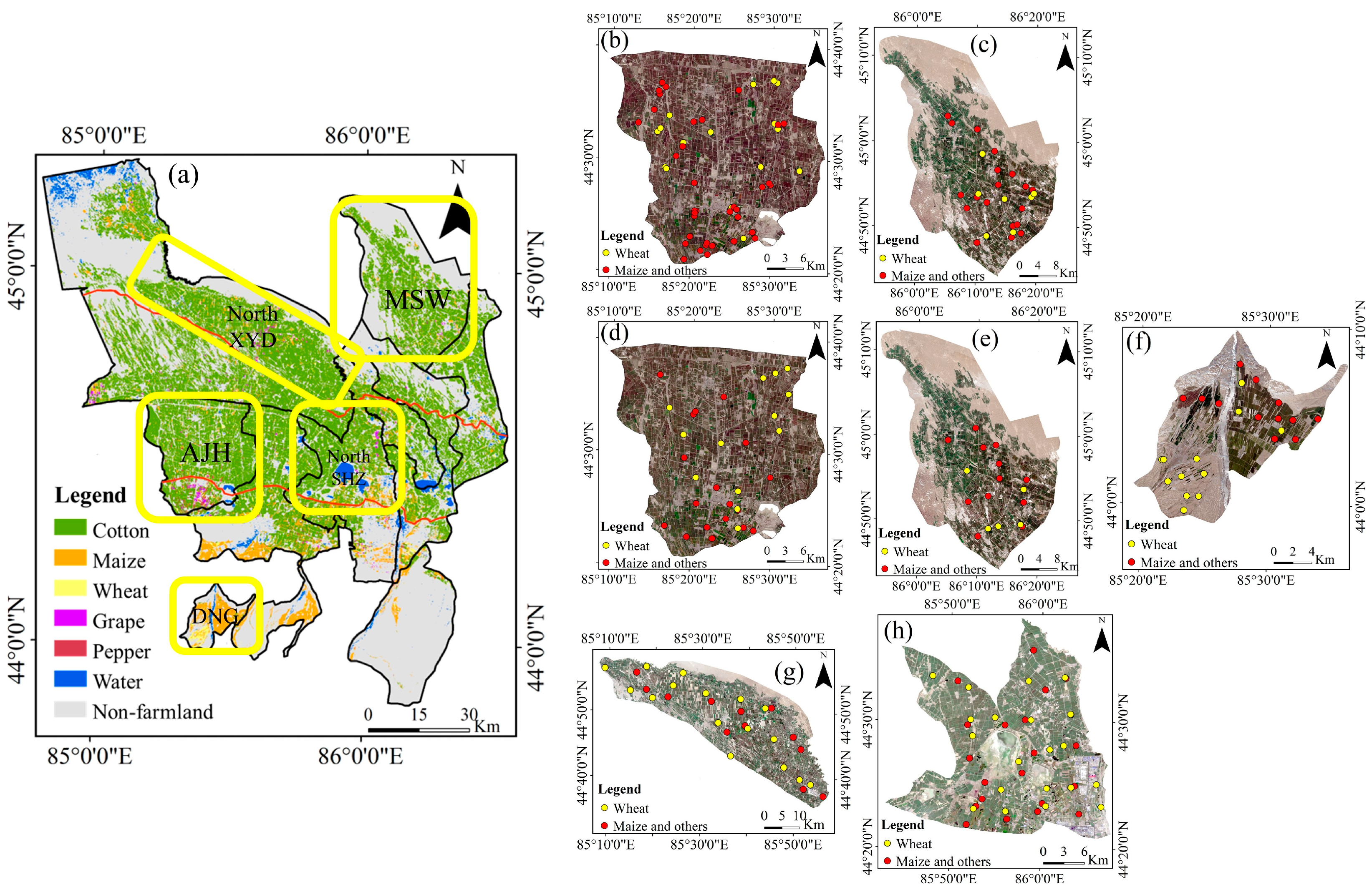
2.2.2. Regional Sampling and Investigation

Regional sampling was carried out during the peak growth stages of wheat and maize over a three-year (2020–2022) period at different locations including the up-, mid-, and downstream sections of the basin. During the first two years, 2020 and 2021, the sampling was conducted in two severely salinized irrigation zones, AJH (midstream) and North MSW (downstream) (Figure 2). Sampling was synchronized with the sampling in cotton fields under FMDI, as detailed in Yang et al. [12]. The scope of the sampling was expanded in 2021 to the upstream DNG irrigation zone (Figure 2). Since most non-salinized farmland is situated in the upstream section and the proportion of samples with SSC lower than ${\phi }_L$ was found to be relatively high in 2020 and 2021, this would inevitably impact the reliability and representativeness of Equation (5). Therefore, in 2022, additional sampling was conducted in North SHZ and North XYD with higher proportion of non-cotton crops and more severe degree of salinization (Figure 2).

In the absence of prior sample data, a regular grid method was used to layout sampling points, with the sampling number n estimated based on the proportion of crop area to study area [40]. Crop area was identified using remote sensing images from the previous year. The 2020–2021 sampling in AJH and MSW focused on cotton fields under FMDI. Due to the low proportion of non-cotton crops, the estimated n was small. To optimize sampling and understand root-zone SSC changes in non-cotton fields, points were not strictly arranged by estimated n. Instead, sampling occurred only if non-cotton farmland was within the sampled cotton field grid. If other crops were present, samples were collected based on crop type. In 2021, non-cotton farmland was more prevalent in DNG, and in 2022, in North XYD and North SHZ, so n was again estimated using the grid method. Consequently, n values for wheat were 24, 34, and 36 for 2020, 2021, and 2022, respectively, while for maize they were 59, 42, and 33. Soil samples were taken from five depths (0–10, 10–20, 20–40, 40–60, and 60–80 cm) near the drip tape. Over three years, 534 soil samples from wheat and 834 from maize were collected, air-dried, ground, and sieved. Electrical conductivity (Swiss Mettler-Toledo S230) was measured using a 1:5 soil–water mass ratio, converted to SSC via a calibration curve, and average root-zone SSC was calculated based on soil depth weighting. Data from 2020 and 2021 aided parameter fitting and model establishment, while 2022 data were for model validation.

2.2.3. Remote Sensing Data Processing

The processing of remote sensing images was mainly used for ground feature classification and ET inversion. Ground feature classification, primarily for crop identification, was conducted on the Google Earth Engine (GEE) cloud platform by combining the simple non-iterative clustering (SNIC) image segmentation algorithm and the random forest (RF) classification algorithm, utilizing multi-temporal images during crop growth periods of each year [32]. To allow rational accuracy for crop identification, Sentinel-2 (5 d, 10 m) and Landsat series remote sensing images with higher spatial and temporal resolutions were selected.

Evapotranspiration inversion was accomplished by combining the SEBS and ESTARFM models. Input data included MODIS (with time and spatial resolutions of 1 d and 1 km, respectively) and Landsat (16 d, 30 m) remote sensing images downloaded during the peak growth stage of the crops, as well as Digital Elevation Models (DEM) and meteorological information. Based on these combined processes of remote sensing fusion and inversion, distributions of ET_a with high spatial and temporal resolution (1 d, 30 m) were obtained [11].

2.2.4. Required Data and Sources for SSC Inversion

(1)

Remote sensing images for ground feature classification: Sentinel images (10 m resolution) were available and used for crop identification from 2018 onward, while Landsat images (30 m resolution) were downloaded for those earlier years’ classification. Given Landsat’s 16-day revisit period, images with less than 10% cloud cover were selected during the April to October growth period from 2001 to 2022. Primarily, single images covering the study area were chosen to reduce errors from stitching; when unavailable, stitching methods were employed [32]. For Sentinel images, although no single image covers the entire area, their shorter revisit period (5 days for Sentinel-2A and 2B) allowed for more frequent data collection. Thus, a monthly NDVI maximum value composite method was used to create one cloud-free or less cloudy image each month [32]. In total, 93 images were collected for classification: 30 from Sentinel-2 and 23, 15, and 25 from Landsat-8, 7, and 5, respectively, using five bands (red, green, blue, near-infrared, and NDVI). Detailed information on the selected images, including datasets in GEE, dates, and bands, is provided in Supplementary Table S1.

(2)

Remote sensing images used for ET inversion: MODIS data (horizontal bands H23 and H24, vertical band V04) comprising daily surface reflectance (MOD09GA) and surface temperature (MOD11A1) from April to September of each year between 2001 and 2022 were sourced from the Level-1 Atmosphere Archive Distribution System (LAADS) Distributed Active Archive Center (DAAC) at the website https://ladsweb.modaps.eosdis.nasa.gov (accessed on 20 December 2022). Further details were described in Qiao et al. [11]. The Digital Elevation Model (DEM) data were obtained from the ASTER GDEM V2 dataset of the Geospatial Data Cloud (http://www.gscloud.cn, accessed on 18 November 2022), Computer Network Information Center, Chinese Academy of Sciences, with a spatial resolution of 30 m.

(3)

Meteorological data: Daily meteorological data needed for the SEBS model [11], including average temperature, maximum temperature, minimum temperature, air pressure, precipitation, wind speed, sunshine hours, and relative humidity from 42 meteorological stations in Xinjiang, spanning from 2001 to 2022, were sourced from the China Meteorological Data Sharing Service System (http://data.cma.cn, accessed on 26 December 2022)).

(4)

Irrigation data: Details such as irrigation method, timing, quantity, and leaching volume of each irrigation zone from 2001 to 2022 were retrieved from Shihezi Irrigation Annual Reports.

2.3. Driving Mechanism Analysis of Spatiotemporal Evolution of Root-Zone SSC

An XGBoost machine learning regression model was established based on root-zone SSC inversion results combined with the analysis of regional water and salt movement principles and correspondingly collected data of influencing factors spanning from 2001 to 2022 in MRB. Subsequently, the TreeSHAP algorithm was applied to assess the contribution of each factor to dynamic changes in root-zone SSC. To analyze and compare the temporal and spatial impact of various factors and offer insights for adjusting planting structure (crop choice and location) and optimizing irrigation, the basin was further divided into 17 partitions based on topography and irrigation zones, as illustrated in Figure 1.

2.3.1. XGBoost Machine Learning Algorithm

The core idea of XGBoost is to sequentially train weak learners (typically decision trees) and combine them into a strong model, with each learner correcting the errors of its predecessor. Regularization helps manage model complexity, while various feature selection strategies and optimizations like parallel processing enhance performance [24]. These attributes make XGBoost effective for classification and regression tasks and popular in machine learning competitions and applications [26].

Model parameters, including learning rate (learning_rate), tree depth (max_depth), and number of estimators (n_estimators), were optimized through a random search algorithm [41] and assessed using 10-fold cross-validation [42]. All operations were conducted using Python 3.9 (Guido Van Rossum, The Netherlands). The specific steps are outlined as follows:

First, the initial parameter ranges were determined according to common scenarios [24]: learning_rate = [0.05, 0.1, 0.5]; max_depth = [3, 4, 5]; n_estimators = [50, 100, 150], which yielded a total of 27 parameter combinations.

Second, each combination was evaluated by randomly dividing the dataset into 10 subsets—nine for training and one for validation—repeated 10 times for different validation sets. Error evaluation was conducted individually for each validation set through the following metrics: coefficient of determination (R²), mean absolute error (MAE), and root mean squared error (RMSE). The average error was determined for each parameter combination.

Finally, the error indicators from cross-validation were compared to identify the combination with minimal error, which was then applied to the entire dataset to build the final XGBoost model, allowing for interpretation via the TreeSHAP algorithm.

2.3.2. SHAP and TreeSHAP Algorithms

The SHAP algorithm, proposed by Lundberg and Lee [22], was employed to analyze the respective contributions of different factors to drive root-zone SSC variations. It enables the explanation of predictions made by various complex black box models based on quantifying the marginal contribution of each feature (i.e., influencing factor). This approach provides a robust basis for interpretability assessment, particularly in the context of environmental data. Given its ability to decompose feature contributions and capture non-linear interactions, SHAP is especially valuable when analyzing complex relationships between various factors, where statistical methods may struggle to provide clear insights [22]. The corresponding mathematical model is generalized as follows:

$$f\left(x\right)\approx g\left(x^{\prime }\right)={\varphi }_0+{\displaystyle \sum _{i=1}^M{\varphi }_i{x}_i^{\prime }},$$

(6)

where x is a specific sample; f(x) is the original prediction model to be explained; x′ is the simplified input of x, with the two variables connected through a mapping function x = h_x(x′), which depends on the selected machine learning model; g(x′) is the explanatory model of f(x); M is the total number of input features; i represents the index of the feature, ranging from 1 to M; $x_i^{\prime }$∈{0,1}^M, {0,1}^M represents a set of M-dimensional vectors composed of 0 and 1, where each vector represents the presence (1) or absence (0) of the feature at the corresponding position; ${\varphi }_i$ is the attribution value (Shapley value) of each feature; ${\varphi }_0$ = E[f(x)] is the baseline value of the explanation model (the mean of prediction results of all samples). For a specific sample x, its Shapely value ${\varphi }_i$ is calculated as:

$${\varphi }_i\left(x\right)={\displaystyle \sum _{S\subseteq N\backslash \left\{i\right\}}\frac{\left|S\right|!\left(\left|M\right|-\left|S\right|-1\right)!}{\left|N\right|!}\left[f_x\left(S\cup \left\{i\right\}\right)-f_x\left(S\right)\right]},$$

(7)

where N is the set of all features in the training set; S represents a feature set, S$\subseteq$N; f_x(S) represents the output of the model for sample x under the given feature set S; f_x(S∪{i}) represents the output of the model for sample x under the given feature set S, plus feature i.

The SHAP algorithm has a solid theoretical foundation, but the high computational complexity of ${\varphi }_i$ limits its practical application. TreeSHAP, a variant of SHAP specifically designed for tree-based models (such as decision trees, random forests, and gradient boosting), offers a more efficient and accurate solution [23]. It decomposes feature contributions through the tree structure and merges them to explain model predictions. Therefore, the TreeSHAP algorithm was used to interpret the XGBoost model with the SHAP 0.41.0 package in Python 3.9.

2.3.3. Data and Sources Required for Driving Mechanism Analysis

Based on the principles of water flow and salt transport in arid regions, root-zone salt accumulation driving mechanisms were analyzed by considering five key categories such as initial condition, geography, plants, meteorology, and human activity. Correspondingly involved specific factors and their data sources are summarized in

Table 1. Factors evaluated for their influence on the spatial and temporal dynamics of root-zone SSC in the Manas River Basin.

Category	Description		Data Source	Time	Abbreviation
Initial SSC	Average root-zone SSC in the previous year		Estimated based on remote sensing images, meteorological data, and irrigation data	2001–2021	Initial SSC
Geography	Soil properties	Soil texture of 0–30 cm	Harmonized World Soil Database dataset (http://www.fao.org, accessed on accessed on 18 November 2022)	—	Top-ST
		Soil texture of 30–60 cm		—	Sub-ST
		Soil bulk density of 0–30 cm		—	Top-SBD
		Soil bulk density of 30–60 cm		—	Sub-SBD
	Altitude		Geospatial Data Cloud (https://www.gscloud.cn, accessed on 18 November 2022)	—	Altitude
Plant	Annual maximum NDVI		Inversely determined based on remote sensing images	2001–2022	NDVI
	Crop area		Inversely determined based on remote sensing images	2001–2022	CA
Meteorology	Total ETa from 1 April to 31 October		Estimated based on remote sensing images and meteorological data	2001–2022	TETa
	Total ET0 from 1 April to 31 October		Calculated based on meteorological data using Penman–Monteith equation	2001–2022	TET0
	Total precipitation from 1 April to 31 October		China Meteorological Data Sharing Service System (http://data.cma.cn, accessed on 26 December 2022)	2001–2022	Pre
Human activity	Planting structure	Proportion of cotton fields	Inversely determined based on remote sensing images	2001–2022	CFP
		Proportion of wheat fields
					WFP
		Proportion of maize (and minority crops) fields
					MFP
	Total irrigation amount from 1 April to 31 October		Irrigation Annual Report of Shihezi City	2001–2022	Irrigation
	Implementation period of FMDI		Obtained year-by-year based on remote sensing inversion of farmland distribution maps	2001–2022	IPF

.

The initial condition refers to the root-zone SSC from the year prior to the study, estimated using remote sensing inversion methods, which incorporated remote sensing images, meteorological, and irrigation data.

In the geography category, five factors were considered: soil texture and bulk density at depths of 0–30 cm and 30–60 cm (representing crop root-zone properties) and the digital elevation model (DEM). Soil data were sourced from the Harmonized World Soil Database (HWSD) of the Food and Agriculture Organization of the United Nations (FAO) (http://www.fao.org, accessed on 18 November 2022), while DEM data came from the Geospatial Data Cloud (https://www.gscloud.cn, accessed on 18 November 2022). Although shallow groundwater significantly affects soil salinity dynamics, most areas in the MRB have groundwater deeper than 2 m, with less than 1% near the spring overflow zone above the local critical threshold (approximately 1.5 m). Moreover, local groundwater depth has gradually increased in recent years [43], so the influence of groundwater was not considered in this study.

Plant factors included the annual maximum NDVI and the total crop planting area. The annual maximum NDVI was derived using the maximum value synthesis method in GEE, while the total crop planting area was determined by analyzing the classification results of remote sensing images.

Meteorological factors were the total ET (TET_a) during the peak growth stage of main crops (April–October), total reference crop ET (TET₀), and total precipitation. TET_a was acquired by accumulating daily ET_a obtained through the remote sensing inversion method [11]; TET₀ was calculated using the Penman–Monteith method [44] and collected daily meteorological data; precipitation was directly retrieved from the China Meteorological Data Sharing Service System (http://data.cma.cn, accessed on 26 December 2022).

Human activity factors encompass five aspects based on local agricultural practices. The first three relate to planting structure, specifically the area proportions of cotton, wheat, and maize, obtained from statistical analyses of remote sensing image classifications. The fourth aspect was the total irrigation amount (per unit area) from April to October, weighted by crop area proportions based on irrigation amounts for each crop in each irrigation zone retrieved from the Shihezi Irrigation Annual Report. The fifth was the implementation period of FMDI (year). With the promotion of FMDI, local salinized soils were reclaimed and cultivated farmland expanded correspondingly [11]. Farmland distribution maps were annually intersected in ArcGIS to quantify areas in 17 partitions, with the average FMDI implementation period weighted by its proportion to total farmland area in each partition. Since widespread FMDI promotion in MRB began in 2001, this year was chosen as the starting point.

As aforementioned, the average impact of each factor was considered for each partition. Except for the relatively stable soil properties and DEM among geographical factors, all other factors varied annually.

2.4. Statistical Analysis

Python 3.9, ArcGIS 10.6 (Exelis Visual Information Solutions, Broomfield, CO, USA), IDL 8.5 (Exelis Visual Information Solutions, Broomfield, CO, USA), and Excel 2016 (Microsoft, Remond, WA, USA) were used for numerical simulations, data, and image processing. Three statistical indices, R², RMSE, and MAE, were applied to evaluate the accuracy of fitting and simulation results [45,46].

3. Results and Discussion

3.1. Estimation and Spatiotemporal Evolution of Root-Zone SSC

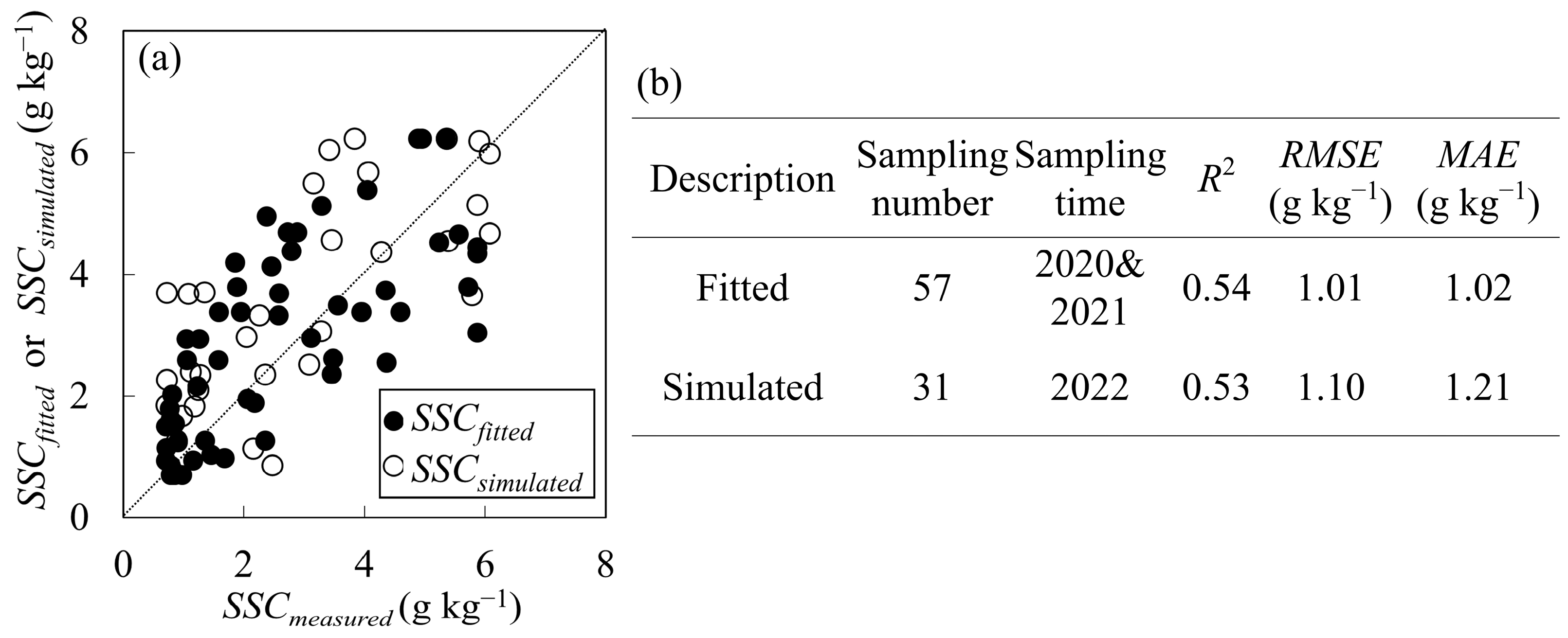
3.1.1. Verification of the Root-Zone SSC Inversion Method in Non-Cotton Fields

Based on distributions of remotely sensed ET_a of wheat and maize fields, the parameter τ in Equation (1) was fitted using measured root-zone SSC (SSC_measured) in 2020 and 2021, and correspondingly fitted values of SSC (SSC_fitted) were obtained. Thereupon, the remote sensing inversion model was used to simulate root-zone SSC (SSC_simulated) in non-cotton fields and validated using measured data in 2022.

Of the 86 sampling points collected for wheat from 2020 to 2022, almost 60% of them (52), with root-zone SSC ranging from φ_L (1.55 g kg⁻¹) to φ_w (8.06 g kg⁻¹), were applicable for parameter fitting (32 in 2020–2021) and accuracy testing (20 in 2022). Among the remaining 34 sample points, 23 measured SSC values were lower than 1.55 g kg⁻¹, primarily located in the upstream DNG irrigation zone, while the SSCs of the other 11 were higher than 8.06 g kg⁻¹, all situated in mid- and downstream irrigation zones with more severe salinization. For maize, out of the 127 sampling points, approximately 69% (88) were suitable for parameter fitting (57) and accuracy testing (31). Among the remaining 39 sample points, 25 had SSC values lower than φ_L (0.70 g kg⁻¹), mostly concentrated in the upstream DNG and South AJH. Conversely, the SSCs of the remaining 14 sample points surpassed φ_w (6.23 g kg⁻¹), all located in more heavily salinized mid- and downstream areas.

The relevant statistical characteristics of sample points with measured SSC falling between φ_L and φ_w for both wheat and maize across different sampling areas over the study periods are presented in

Table 2. Statistical characteristics of measured root-zone SSC of non-cotton fields in typical irrigation zones from 2020 to 2022.

Year	Sampling Area	Crop	Sampling	Maximum	Minimum	Mean
			Number	g kg−1	g kg−1	g kg−1
2020	AJH, MSW	Wheat	18	7.83	1.55	4.04 ± 1.92
		Maize (and others)	35	5.87	0.73	2.57 ± 1.80
2021	DNG, AJH, MSW	Wheat	14	7.73	1.59	3.98 ± 1.78
		Maize (and others)	22	5.35	0.72	2.46 ± 1.57
2022	North XYD, North SHZ	Wheat	20	7.86	1.62	4.74 ± 2.18
		Maize (and others)	31	6.08	0.72	2.95 ± 1.87

. Regarding wheat, the minimum and maximum values of SSC observed over the years closely resemble φ_L and φ_w, respectively. However, the average values fluctuated significantly. In 2020, samples were collected from AJH and North MSW irrigation zones with relatively severe salinization, thus yielding an average SSC of about 4.04 g kg⁻¹. Subsequent sampling in 2021 supplemented a few points from DNG in lower salinized upstream, resulting in a slight decrease in the average SSC to around 3.98 g kg⁻¹. Recognizing the insufficiency of sample points with SSC values in the range of φ_L − φ_w suitable for model testing (caused by too many sample points with SSC less than φ_L) in 2020 and 2021, additional sampling work was conducted in more heavily salinized North XYD and North SHZ for non-cotton fields, leading to the highest average SSC of about 4.74 g kg⁻¹. For maize, the observed minimum and maximum SSC values were also similar to φ_L and φ_w, respectively. Notably, the average SSC was still the highest in 2022 (2.95 g kg⁻¹), followed by 2020 (2.57 g kg⁻¹), and lowest in 2021 (2.46 g kg⁻¹). Lower values of SSC were generally observed for maize compared to wheat, which could also be attributed to different mulching conditions at the soil surface. Non-mulched surfaces in wheat fields would be expected to experience greater evaporation and upward movement of soil water, consequently increasing root-zone SSC.

The parameter τ in Equation (1) was fitted as 1.41 for wheat using sampling data from 2020 and 2021. Comparisons between SSC_fitted and SSC_measured revealed correlation (Figure 3a), with R², RMSE, and MAE of 0.57, 1.39 g kg⁻¹, and 1.20 g kg⁻¹, respectively (Figure 3b). Verification based on sampling data in 2022 further confirmed the inversion model’s accuracy in estimating root-zone SSC of wheat, with R², RMSE, and MAE of 0.54, 1.49 g kg⁻¹, and 1.26 g kg⁻¹, respectively, between SSC_simulated and SSC_measured. Similarly, the index τ was optimized as 2.49 for maize. Probably affected by multiple crop mixtures, the R² for both fitting and verification processes were slightly lower than those of wheat but still within an acceptable range (Figure 4). Smaller values of RMSE and MAE were observed due to the lower measurements of SSC and the narrower range between φ_L and φ_w for maize (0.70–6.23 g kg⁻¹) compared to wheat (1.55–8.06 g kg⁻¹). Notably, comparison results showed that the value of R² was even as low as 0.53 in this study. Referring to the suggested R² value of ~0.5 for a moderate correlation by De Santis et al. [47] and recommendation of R² > 0.5 for acceptable basin-scale inversion by Li et al. [48], we believe that the proposed inversion method should be considered to be reasonable and reliable in estimating regional farmland root-zone SSC variations, with limiting error in an acceptable range, due to the complex and multifaceted nature of the factors involved.

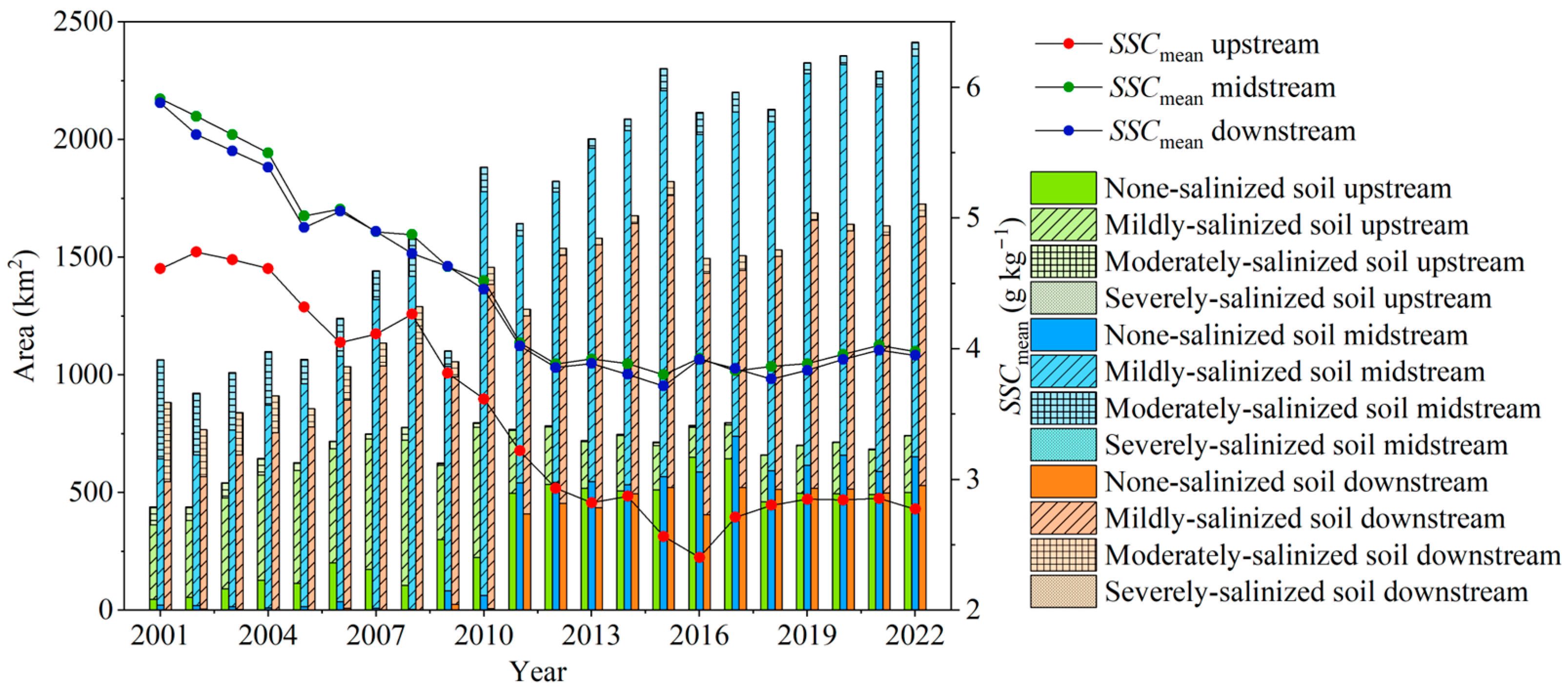
3.1.2. Dynamic Evolution of Root-Zone SSC Distributions

With the crop identification results obtained through integrating SNIC and RF algorithms (Supplementary Materials Figure S1), distributions of root-zone SSC for both cotton and non-cotton fields in MRB from 2001 to 2022 were determined based on daily ET_a with 30 m resolution derived from the coupled model of SEBS and ESTARFM, along with the irrigation amount for each irrigation zone obtained through regional surveys and meteorological data from Hutubi meteorological station (Figure 1). Estimated distributions of root-zone SSC for the years 2002, 2007, 2011, 2017, and 2022 are depicted in Figure 5. Following the classification standard for salinized soils in arid and desert regions of Xinjiang, the root-zone soil was categorized into four groups: non-salinized (SSC < 3 g kg⁻¹), mildly-salinized (3–6 g kg⁻¹), moderately-salinized (6–10 g kg⁻¹), and severely-salinized (SSC > 10 g kg⁻¹), consistent with the previous study of Yang et al. [12]. For a specific crop type, if the simulated SSC was less than φ_L, it was set as φ_L during the simulation process, since values of SSC lower than φ_L were meaningless for the model. Similarly, simulated SSC values exceeding φ_w were adjusted to φ_w.

Due to the dominance of cotton fields in MRB, root-zone SSC distributions for all farmlands closely resembled those for cotton fields, especially in mid- and downstream areas. In contrast, the upstream region, where non-cotton crops prevail, showed notable differences. Due to the higher φ_L of cotton compared to the other two types of crops, the salinization level in the upstream region, originating with lower salinity, tended to decrease dramatically when non-cotton cropland was considered. While previous studies extensively analyzed root-zone SSC dynamics for cotton [12], a concise summary for all farmlands in the basin is as follows:

Average root-zone SSC in local farmlands decreased significantly from 5.47 g kg⁻¹ (Figure 5a) to 3.77 g kg⁻¹ (Figure 5e) from 2001 to 2022, with an average annual decrease of approximately 1.5% (0.08 g kg⁻¹). This trend generally followed two different stages. Prior to 2011, SSC dropped sharply from 5.47 to 3.82 g kg⁻¹, with an average annual decrease of around 0.18 g kg⁻¹. From 2011 to 2017, SSC fluctuated slightly, decreasing by 0.2 g kg⁻¹ (3.82 to 3.62 g kg⁻¹) before rising to 3.77 g kg⁻¹ by 2022.

Spatially, mid- and downstream salinization levels were similar and significantly higher than those upstream, with average SSC about 0.81 g kg⁻¹ higher (Figure 6), likely due to better soil texture and water conditions upstream. The average SSC upstream fell from 4.59 g kg⁻¹ in 2002 to 3.05 g kg⁻¹ in 2022, with an average annual decrease of 1.6% (0.07 g kg⁻¹). Before 2007, most areas, except for the southern mountains with non-salinized soil, had mildly-salinized soil (Figure 5a,b). By 2007, approximately 554.09 km² (74.2%) of the upstream crop area was mildly salinized (Figure 6). Continuous reclamation and irrigation transformed the upstream soil to non-salinized by 2011 (Figure 5c). By 2022, non-salinized soil expanded to about 499.83 km² (67.3%) upstream. The average root-zone SSC in the mid- and downstream regions decreased from 5.69 g kg⁻¹ in 2002 to 3.89 g kg⁻¹ in 2022, at an annual rate of 1.5% (0.08 g kg⁻¹). In 2002, these areas were primarily mildly- and moderately salinized, with midstream soils covering approximately 621.04 km² and 421.97 km² of mildly and moderately salinized soil (over 97.8% of farmlands), and downstream soils at about 545.45 km² and 337.24 km² (nearly 100% of farmlands) (Figure 6). By 2007, nearly all soils were mildly salinized, covering approximately 1311.56 km² (90.9%) midstream and 1036.31 km² (91.3%) downstream (Figure 6). As farmland reclamation progressed, overall salinization in the region decreased, leading to a gradual increase in non-salinized soil (see Figure 5c,d for 2011–2017). However, due to limited water availability, unmet irrigation and leaching needs reversed the decline in soil salinity, causing an expansion of mildly salinized areas from 2017 onward [12]. Consequently, a slight increase in average root-zone SSC in the mid- and downstream areas was observed when comparing 2022 to 2017 (Figure 6).

3.2. Driving Mechanisms for Root-Zone SSC Evolution

3.2.1. Parameter Optimization and Accuracy Evaluation of the XGBoost Model

The XGBoost model was optimized using the approach of 10-fold cross-validation and random search, yielding the parameters of: learning_rate = 0.1, max_depth = 5, n_estimators = 100. As depicted in Figure S2, predicted root-zone SSCs (SSC_predicted) were highly correlated with their measured values (SSC_measuted), with R² as high as 0.96 ± 0.01, indicating the robust explanatory power of the XGBoost model. Additionally, the low values of RMSE (0.19 ± 0.03 g kg⁻¹) and MAE (0.14 ± 0.02 g kg⁻¹) suggested that the predicted SSC was consistent with its target value.

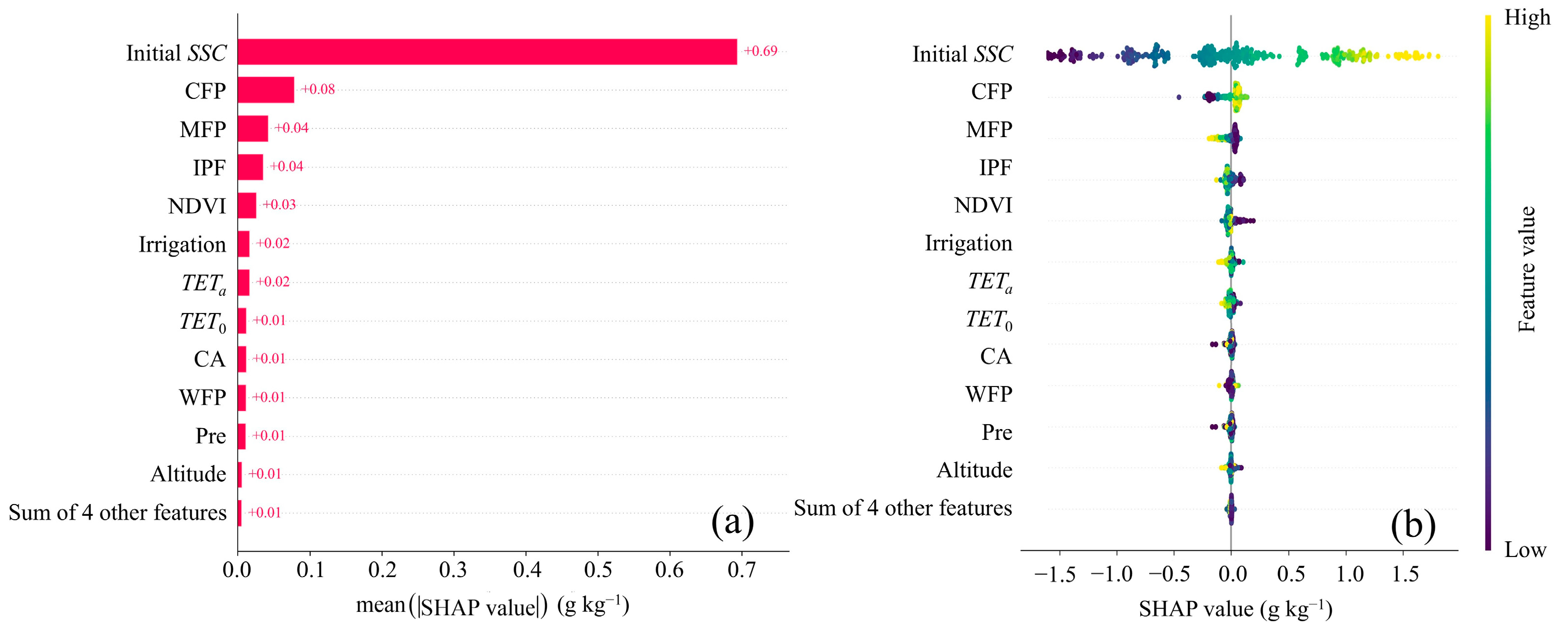
3.2.2. Overall Assessment of Influencing Factors Based on the TreeSHAP Algorithm

In Section 2.3.1, the optimized parameter combination was used to build the final XGBoost model for analyzing the contributions of factors affecting root-zone SSC via the TreeSHAP algorithm.

As described in Section 2.3.1, the optimized parameter combination was applied to the entire dataset to construct the final XGBoost model, so as to provide effective information for further insights into the contributions of various factors affecting root-zone SSC through the TreeSHAP algorithm. This algorithm quantifies each factor’s contribution through SHAP values, interpreting predictions as the sum of these contributions [23]. Figure 7a,b illustrates the SHAP bar and summary plots, where the bar plot ranks feature importance based on absolute SHAP values, while the summary plot shows individual SHAP values, indicating how each factor affects predictions relative to the baseline. Together, these plots highlight the global significance of various features.

Initial SSC exerted the most substantial impact on the predicted SSC value of the assessment year, with a mean ($\left|\mathrm{SHAP} \mathrm{value}\right|$) of 0.69 g kg⁻¹ (Figure 7a). Due to limited precipitation, root-zone SSC leaching in MRB primarily depends on irrigation. Local water resource scarcity has facilitated the development and adoption of water-saving FMDI technology. Undoubtedly, high frequency and low quota FMDI would not be conducive to the leaching of root-zone SSC. Therefore, the initial SSC occupied the absolutely highest impact position.

Cotton (CFP) and maize (MFP) proportions in the planting structure were the second and third significant factors affecting SSC dynamics, with mean ($\left|\mathrm{SHAP} \mathrm{value}\right|$) reaching 0.08 and 0.04 g kg⁻¹, respectively (Figure 7a). As the dominant crops (85% CFP and 11% MFP from 2002 to 2022), their spatial distributions explain variations in SSC across regions. Maize, with low temperature requirements and poor salt tolerance, thrived in cooler, slightly salinized upstream areas, benefiting from low initial salinity and good drainage. In contrast, mid- and downstream regions, with fine-textured soils and insufficient water supply, faced higher salinization, leading to more cotton cultivation, which prefers light and heat. Consequently, higher SSC values were linked to increasing CFP and decreasing MFP. Wheat (WFP) had minimal influence, ranking 10th with a mean ($\left|\mathrm{SHAP} \mathrm{value}\right|$) of only 0.01 g kg⁻¹ (Figure 7a), due to its low planting fraction of just 4% over 22 years (Figure 7a).

The implementation period of FMDI (IPF) significantly influenced SSC predictions, with a mean ($\left|\mathrm{SHAP} \mathrm{value}\right|$) of 0.04 g kg⁻¹ (Figure 7a). This relationship indicates that a longer IPF enhances the impact of irrigation on SSC. While FMDI is praised for its water-saving and salt-inhibiting benefits, alternating it with traditional flood irrigation can weaken centralized salt leaching. Initially, during a short IPF, salts in the upper root-zone are effectively leached, but long-term IPF may result in salt accumulation in the lower root-zone. Previous research showed that root-zone SSC typically decreases during the first 10–12 years of FMDI implementation before stabilizing or increasing [49,50], a trend also observed in this study (Figure S3d).

As shown in Figure 7a, NDVI was the fifth most important factor affecting SSC, with a mean ($\left|\mathrm{SHAP} \mathrm{value}\right|$) of 0.03 g kg⁻¹. As a common remote sensing indicator of vegetation coverage and health, NDVI’s significance is expected given its close relationship with crop growth [51]. The effects of irrigation amount (irrigation) and TET_a on SSC were similar, both with a mean ($\left|\mathrm{SHAP} \mathrm{value}\right|$) of 0.02 g kg⁻¹ (Figure 7a). In the arid MRB, TET_a largely depends on irrigation, making it a key factor in root-zone SSC dynamics. During peak growth stages, irrigation typically met crop water needs, with stable total irrigation amounts across different growth seasons. Prior to 2012, crop water demand satisfaction exceeded 80% in most MRB areas [32], with water consumption TET_a generally above 530 mm (Figure S3g). Consequently, the statistical data for irrigation and TET_a showed relatively weak influence on SSC. The irrigation amount was calculated based on the planting ratios of the three crop types, and the true impacts of irrigation and TET_a were reflected in related factors such as CFP, MFP, IPF, and NDVI.

Among the considered features, TET₀, crop area (CA), WFP, precipitation (Pre), and altitude had low impact on the model, each with a mean of 0.01 g kg⁻¹ (Figure 7a). TET₀ is largely determined by meteorological conditions, showing minimal spatial variability, with total fluctuations not exceeding 165 mm (less than 19% of its lowest value) (Figure S3h). While CA increased significantly by 118% (2568 km²) from 2001 to 2022 (Figure S3i), most growth occurred before 2015, limiting its later impact on SSC. WFP and precipitation were both low, with little variability. Additionally, constant altitude and geographical factors, like soil texture and bulk density, minimally affected SSC variations. In summary, the primary driver of root-zone SSC dynamics in MRB was initial SSC, followed by planting structure (mainly CFP and MFP), IPF, and irrigation, with NDVI and TET_a also influencing variations.

While initial SSC was the most significant contributor, other factors also played important roles in SSC dynamics. As shown in Figure 7b, high initial SSC and CFP values resulted in positive SHAP values, indicating a positive correlation with predicted SSC values, whereas low values corresponded to negative SHAP values. Conversely, factors like IPF, MFP, TET_a, NDVI, irrigation, and TET₀ showed a negative correlation. These correlation relationships are consistent with water flow and salt transport principles in arid regions. For instance, higher initial SSC complicates salt leaching, increasing predicted root-zone SSC, while higher values of the other factors suggest better irrigation and salt leaching, thus decreasing SSC. Additionally, cotton, with moderate salt tolerance, was mainly planted in more saline mid- and downstream areas, while maize thrived in less saline upstream regions, leading to a positive correlation for CFP and a negative correlation for MFP with SSC. However, the relationships between feature values and predicted SSC in Figure 7a,b are preliminary; a deeper understanding requires scientific analysis of the internal relationships, partially explored through SHAP dependence plots.

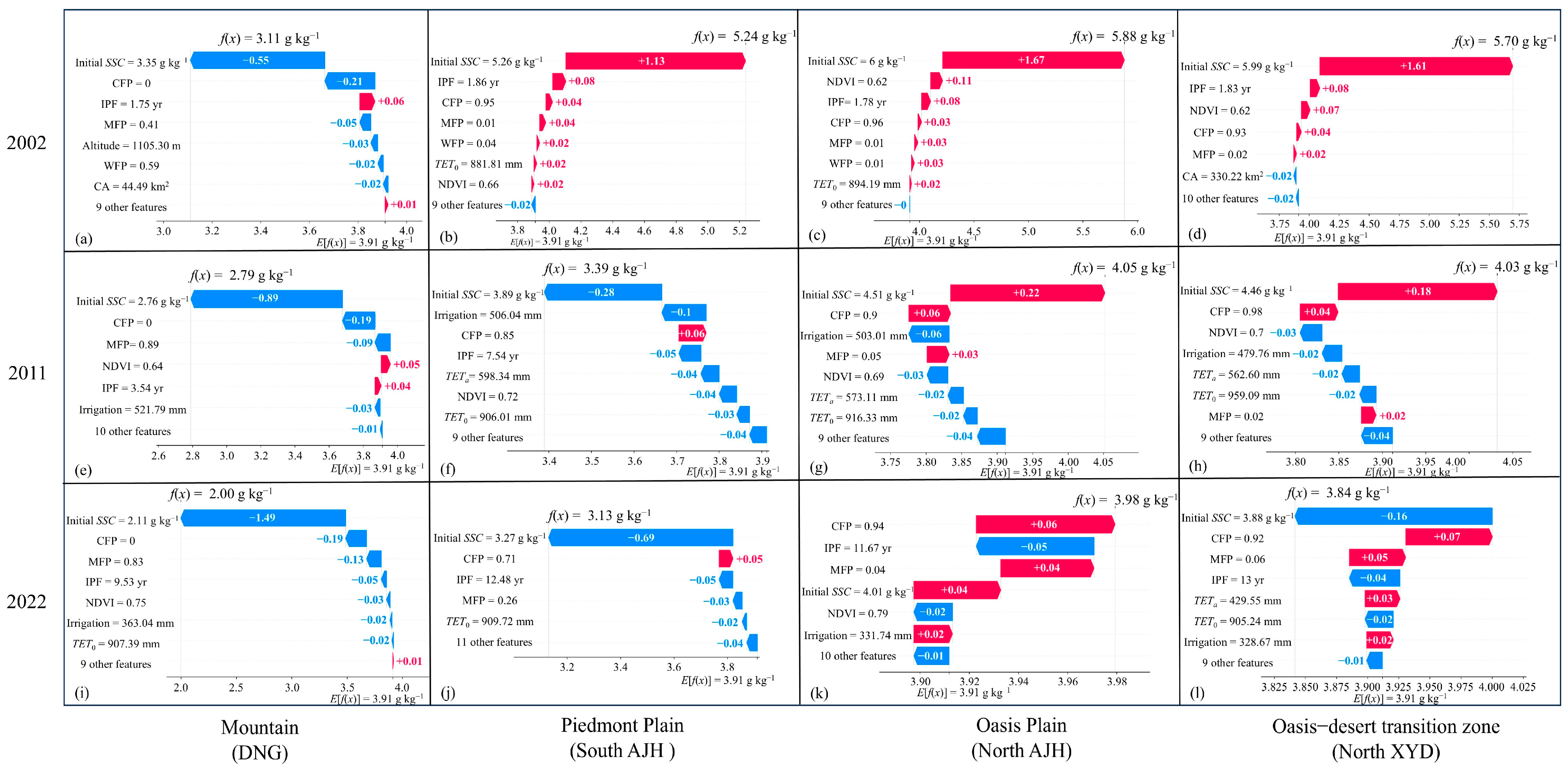
3.2.3. Further Interpretation on the Driving Mechanisms of SSC

The SHAP dependence plots provide a detailed evaluation of how each factor influences SSC variations, highlighting both linear and nonlinear relationships as well as interactions between factors. Figure 8 presents the top seven influencing factors with mean ($\left|\mathrm{SHAP} \mathrm{value}\right|$) ≥ 0.02 g kg⁻¹. The plots display the quantitative relationship between SHAP values and feature values, using a color bar to show interaction patterns with the most related features, enhancing understanding of these interactions. The influencing factors are broadly classified into two categories: natural conditions (initial SSC, NDVI, and TET_a) and human activities (CFP, MFP, IPF, and irrigation), as shown in Table 1. Out of the total 0.98 g kg⁻¹ for the sum of mean ($\left|\mathrm{SHAP} \mathrm{value}\right|$), 93.9% (0.92 g kg⁻¹) was explained by the top seven factors, with 75.5% (0.74 g kg⁻¹) driven by natural factors and 18.4% (0.18 g kg⁻¹) by human activities (Figure 7a). To clarify the driving mechanisms in Figure 8, the specific impacts of these factors are assessed according to these two categories.

(1) Natural Conditions:

As outlined in the study area overview, significant variations in natural conditions like soil texture, salinity, irrigation, and drainage exist across the up-, mid-, and downstream regions of the basin, critically affecting SSC. The sum of mean ($\left|\mathrm{SHAP} \mathrm{value}\right|$) of natural conditions was about four times that of human activities, in which initial SSC played the greatest role, accounting for about 93.2% of the 0.74 g kg⁻¹ SSC variations in natural conditions (Figure 7a). Due to low precipitation and limited drip irrigation, root-zone SSC changed gradually over time, with minimal fluctuations within a growing season (year). As a result of regional distribution, i.e., almost always remaining lowest in the mountainous areas, higher in the piedmont plains, and highest in the mid- and downstream areas, initial SSC emerged as the primary driver of SSC variations. Over the past two decades, areas with high initial SSC consistently showed higher predicted SSC values, with SHAP values increasing nearly linearly with initial SSC (Figure 8a). The wide SHAP range (−1.5 to 1.75 g kg⁻¹) indicated its significant impact on the model. Initial SSC also strongly interacted with factors like CFP, MFP, IPF, irrigation, and TET_a (Figure 8b–d,f,g). Notably, initial SSC was influenced by human activities, with IPF as the most significant interactive factor. Longer IPF would increase irrigation water amount for salt leaching and thereby exert a more pronounced influence on root-zone SSC (i.e., provide an initial condition for the subsequent year). Consequently, initial SSC gradually decreased with rising IPF, showing a general downward trend in SSC levels across MRB over the past two decades.

Both NDVI and TET_a, key factors related to crop growth, indirectly influenced SSC dynamics through the impact from irrigation, a major human activity. As shown in Figure 8e and g, when NDVI < 0.73 (with IPF mostly < 8 years) and TET_a > 550 mm, corresponding to pre-2011 (Figure S3e,g), farmland reclamation relied on abundant irrigation (average 470 ± 29 mm, Figure S3f). During this period, NDVI was experiencing rapid growth, leading to decreasing SHAP values (lower predicted SSC) with increasing NDVI (Figure 8e). Meanwhile, due to ample irrigation, TET_a remained consistently high with low variability between partitions (Figure S3g), limiting its impact on SSC, as reflected by SHAP values near zero (Figure 8g). Post-2011, as NDVI surpassed 0.73 (with IPF > 8 years) and TET_a dropped below 550 mm, land expansion slowed due to limited available arable land, leading to minimal NDVI growth and little influence on SSC (Figure 8e). Additionally, the continuous expansion of agricultural land contributed to a decline in irrigation (average 371 mm from 2012–2022, Figure S3f), which suppressed TET_a, with lower TET_a values correlating to higher SHAP values or predicted SSCs (Figure 8g).

(2) Human activity

The driving contribution of human activity factors (concentrated on CFP, MFP, IPF, and irrigation) on SSC variations should also not be underestimated. Almost all the impact of human activity from the four factors was closely related to the development of FMDI, expansion of planting areas, and decrease in irrigation quota over the past 20 years in the MRB. Undoubtedly, the impact of human activity was inseparable from the interaction with natural conditions, as demonstrated by the strongest interactions between natural Initial SSC and the four listed human activity features.

Due to lower accumulated temperatures and other factors, upstream areas were less suitable for cotton but better for maize. As a result, cotton was rarely planted, and CFP in the upstream mountainous and piedmont plains averaged about 40% ± 33% over 21 years, often below 70% (Figure S3b). Conversely, MFP exceeded 25%, averaging 48% ± 28% (Figure S3c). In the mid- and downstream areas, where soil salinity was higher, cotton, a salt-tolerant crop, was predominantly grown. About 90% of the 210 data points from these areas had CFP above 80%, averaging 90% ± 9% (Figure S3b), while MFP was below 20%, averaging 6% ± 7% (Figure S3c). In upstream regions (CFP < 70%, MFP > 25%), initial SSC was generally below 3.5 g kg⁻¹. The SHAP values for CFP were predominantly negative and increased with rising CFP (Figure 8b). Conversely, for MFP, the SHAP values were also negative but decreased as MFP increased (Figure 8c). This indicated that in the upstream regions, the lower the CFP and the higher the MFP, the lower the predicted SSC values would be. In the mid- and downstream regions (CFP > 70% and MFP < 25%), the initial SSC was generally higher than 3.5 g kg⁻¹, and the SHAP values for both CFP and MFP were positive but close to zero (Figure 8b,c). This indicated that, compared to the upstream regions, the predicted SSC values were higher. However, due to the relatively small range of variation in both CFP and MFP, their impact on SSC was limited.

The impact of IPF on SSC was closely linked to irrigation changes. While some farmlands had IPF lasting up to 22 years, this study averaged IPF across partitions, yielding durations of 1–16 years (Figure S3d). Before 2011, when IPF was under 8 years and irrigation was higher, the SHAP value (predicted SSC) decreased as IPF increased (Figure 8d). After 2011, with reduced irrigation and less leaching, the increase in IPF had minimal impact on lowering SSC (Figure 8d).

Irrigation decreased after 2011 but remained above 400 mm until 2013 (Figure S3f), with notable partition differences: higher up- and midstream values compared to downstream. Consequently, SHAP values were primarily negative, significantly decreasing with increased irrigation (Figure 8f). After 2013, as cotton fields expanded, irrigation dropped below 400 mm (Figure S3f), becoming insufficient for salt leaching, and partition differences narrowed, especially between mid- and downstream. This reduced irrigation’s effectiveness in lowering SSC, causing SHAP values to approach or exceed 0. Although SHAP values continued to decline with increased irrigation (Figure 8f), the trend’s magnitude was small, indicating a limited decrease in SSC. Overall, with a narrow irrigation range (approximately 500–330 mm) and ample supply during peak growth, irrigation’s contribution to predicted SSC ranked only sixth (Figure 7a). However, as a key regulatory factor in human activities, its variations may indirectly influence other natural and human factors.

3.2.4. Spatiotemporal Changes of Main Influencing Factors and Their Impacts

To analyze the spatial and temporal variations of factors influencing root-zone SSC, four representative partitions were selected: DNG in the upstream mountains, South AJH in the upstream piedmont plain, North AJH in the oasis plain, and North XYD in the oasis–desert transition zone. The SHAP waterfall plots for 2002, 2011, and 2022 were examined, focusing on features with SHAP values above 0.02 g kg⁻¹ to highlight the seven top influencing factors from Section 3.2.3. The plots depict the transition of each influencing factor from the model’s baseline to the final predicted SSC, with predicted values on the horizontal axis and features arranged by their influence on the vertical axis. Blue bars indicate positive SHAP values, while red bars indicate negative ones. The model’s baseline value, E[f(x)], was 3.91 g kg⁻¹, where f(x) represents the final predicted SSC calculated by summing the baseline and SHAP values, reflecting the overall impact of each feature on SSC predictions.

Unlike the other three partitions, DNG in the upstream mountains has unique natural characteristics, including high altitude, coarse soils, low salinity, and favorable irrigation/drainage conditions. Consequently, its initial SSC was approximately 2.50, 1.03, and 1.65 g kg⁻¹ lower than the average of the other three partitions in 2002, 2011, and 2022, respectively (Figure S3a). The CFP in DNG remained at 0 due to unsuitable conditions for cotton planting, while the other three partitions maintained CFP levels above 70% annually (Figure S3b). However, DNG exhibited a higher MFP, approximately 40%, 83%, and 71% greater than the other partitions in 2002, 2011, and 2022, respectively (Figure S3c). These factors—initial SSC, CFP, and MFP—were the main drivers behind the decline in predicted SSC in DNG (Figure 9a,e,i). Additionally, IPF, NDVI, and irrigation displayed significant temporal but minimal spatial variations. All were negatively correlated with predicted SSC, resulting in increased SSC with lower values and decreased SSC with higher values. For example, in 2002 and 2011, IPF and NDVI values were below 3.54 years and 0.64, respectively, contributing to varying increases in predicted SSC (Figure 9a,e). In contrast, by 2022, IPF and NDVI rose to 9.53 years and 0.75, leading to a notable decrease in predicted SSC (Figure 9i). Regarding irrigation, the abundant water supply in 2011 resulted in a peak irrigation amount of 521.79 mm—about 60 mm higher than that in 2002—causing a decrease in predicted SSC even in upstream areas (Figure 9e). This trend was more pronounced in the other three partitions with poorer water supply and drainage (Figure 9f,g,h). Despite irrigation decreasing to 363 mm by 2022, it continued to drive SSC down in the mountainous upstream area, likely due to a more sufficient water supply, with irrigation amounts about 30 mm higher than the average of the other three partitions (Figure S3f).

The upstream piedmont plain where the South AJH is located acts as a transitional zone between the basin’s mountainous and lower regions, maintaining an intermediate SSC level. Unlike the upstream mountainous areas, significant spatial variations were observed in the three main factors affecting predicted SSC—initial SSC, CFP, and MFP—at the century’s start. An elevated initial SSC (5.26 g kg⁻¹), high CFP (95%), and low MFP (1%) contributed to increased predicted SSC (Figure 9b). However, with the ongoing implementation of FMDI, the initial SSC in this area significantly decreased over two decades, falling below the baseline value of 3.91 g kg⁻¹ by 2011 and leading to a gradual decline in predicted SSC. By 2022, CFP had dropped to 71%, while MFP increased to 26% (Figure 9j), primarily due to the low salinization level, which allowed for diverse crop cultivation. The South AJH became a key region where the cultivation area of cotton was reduced while the area of alternative crops expanded. Despite this, CFP remained higher than in mountainous areas, leading to a consistent increase in predicted SSC. Conversely, the rising MFP contributed to a decline in predicted SSC in 2022, likely due to maize’s lower salt tolerance and higher irrigation needs compared to cotton. For instance, in 2002, South AJH’s irrigation amount was similar to that of North AJH and North XYD, which cultivated more cotton; by 2022, it was approximately 30 mm higher (Figure S3f). Other factors, such as IPF, NDVI, irrigation, and TET_a, exhibited minor spatial variations but significant temporal fluctuations, negatively correlating with SSC. Low values of these factors drove increases (or decreases) in SSC. For example, in 2002, low IPF (1.86 years) and NDVI (0.66) resulted in predicted SSC increases of 0.08 and 0.02 g kg⁻¹, respectively (Figure 9b). Unlike DNG, the crop area in South AJH steadily expanded. By 2011, IPF rose to 7.54 years, and NDVI increased to 0.72, contributing to decreasing SSC (Figure 9f). The rise in irrigation in 2011 to 506.04 mm—about 40 and 160 mm higher than in 2002 and 2022, respectively (Figure 9f)—also led to a noticeable decrease in predicted SSC. The corresponding increase in TET_a due to higher irrigation further drove down SSC.

The SSC levels in North AJH (midstream oasis plain) and North XYD (downstream oasis–desert transition) were similar, with North AJH showing a slight increase due to the shallow groundwater from midstream spring overflow (Figure 9c,d,g,h,k,l). The analogous natural conditions between the two regions led to a comparable influence of each factor. In 2002, predicted SSC for both areas exhibited a general upward trend compared with the base value like the upstream South AJH, driven by two main categories of factors: spatially variable factors like initial SSC (around 6 g kg⁻¹), CFP (95%), and MFP (1.5%), and temporally dynamic factors such as IPF (1.81 years) and NDVI (0.62), which negatively correlated with SSC (Figure 9c,d). Planting structure differences between the two regions were minimal, with CFP and MFP consistently driving SSC increases. However, due to FMDI and expanding planted areas, initial SSC in both regions decreased over 20 years. By 2022, North XYD’s initial SSC fell below the baseline to 3.88 g kg⁻¹, leading to a predicted SSC decrease (Figure 9l). Meanwhile, IPF and NDVI gradually increased, becoming key factors in reducing predicted SSC by 2011 and 2022. In contrast to the upstream areas, irrigation had a greater impact on SSC in the more salinized mid- and downstream regions. Higher irrigation (correspondingly resulting in higher TET_a) in 2011 had a significant effect on the reduction in SSC. However, as the planting area expanded and could not be sufficiently irrigated, consequentially decreased irrigation served to reverse the predicted SSC to an increasing trend. By 2022, irrigation in these two regions dropped to 330 mm, much lower than upstream, resulting in a slight 0.02 g kg⁻¹ increase in predicted SSC (Figure 9k,l). This highlights the need for vigilance in mid- and downstream areas of MRB regarding the risk of secondary salinization due to reduced water supply for irrigation and salt leaching.

3.2.5. Possible Regulatory Measures Based on Driving Mechanism Analysis

This study quantitatively analyzed the effects of 16 features, including initial SSC, IPF, planting structure, irrigation amount, NDVI, and TET_a, on dynamics of root-zone SSC across 17 partitions in MRB. Among them, planting structure (including CFP, MFP, and WFP) and irrigation represent the main human activity regulatory measures. Therefore, the revealed SSC spatiotemporal evolution and its driving mechanism analysis can serve to recommend future several regulatory measures.

Terrain and topography are key factors in soil salinization across the MRB. From south to north, the region consists of the Tianshan mountains, piedmont plain, oasis plain, and oasis–desert transition area. Salinity is lowest in the Tianshan mountains, slightly higher in the piedmont plain, and highest in the mid- and downstream oasis and oasis–desert areas, which face similar salinity challenges. The upstream mountainous region, with low salinity, coarse soils, and good irrigation/drainage, does not require much intervention. The cold climate here limits cotton cultivation, and the cultivation areas of maize and wheat can be expected to increase in the future. The piedmont plain, though the salinity level is slightly higher than the mountains, is suitable for diverse crops. Salt-sensitive economic crops like chili peppers and tomatoes are recommended here. In contrast, the oasis plain and oasis–desert transition face severe salinization due to low elevation, poor drainage, and limited water supply. While FMDI technology has reduced root-zone salinity over the past two decades, the rapid expansion of cotton cultivation has decreased irrigation per unit area, reducing TET_a and reversing the salinity decline. To address this, reducing cotton cultivation and maintaining or increasing irrigation per unit area is recommended to effectively leach salt and prevent further increases in root-zone salinity.

As previously mentioned, there is an increasing conflict between water availability and demand in the MRB. Given that it is impossible to increase the local water supply, the expansion of irrigated areas must be constrained by available water resources to optimize benefits and promote ecological sustainability. Agricultural planting patterns should, therefore, be based on the region’s total water availability. Using the ten partitions in the heavily salinized mid- and downstream MRB (Figure 2, North AJH, North JGH, South XYD, South XHZC, South MSW, North MNS, North SHZ, North MSW, North XYD, North XHZC) as examples, a scenario simulation was conducted to examine the impact of adjusting planting structure on root-zone SSC. Compared to 2017 with the highest irrigation quota and relatively low root-zone SSC in the past 6 years, the irrigation amount per unit area in 2022 would need to be increased by 20 mm. Assuming the total irrigation water supply and non-cotton crop areas remain unchanged, the cotton planting area across the ten partitions would need to decrease by 147.21 hm², with reductions ranging from 1.12 to 37.45 hm² per partition (rebalanced based on irrigation amounts). Using the well-trained XGBoost model and adjusting factors such as a 1% decrease in CFP in six partitions, a 1% increase in MFP in three, and a 1% decrease in WFP in one, root-zone SSC in 2022 was re-predicted. The results showed decreases in SSC_predicted across all ten partitions, ranging from 0.01 to 0.06 g kg⁻¹ (Figure S4), with the largest reduction in North MNS, where SSC dropped from 3.97 to 3.91 g kg⁻¹. This highlights the insufficiency of current irrigation levels in the mid- and downstream regions, posing a risk of root-zone salt accumulation. Addressing this issue without reducing cultivated areas would require a careful increase in irrigation to ensure effective salt leaching.

However, constrained by the quality and coverage of regional sampling data and the simplicity of the scenario simulation design for root-zone SSC, findings in this study are preliminary. Their applicability and reliability are usually expected to be enhanced through extensively cross-regional validations under more complicated practical environments. In addition, more extensive field experimental data should also be helpful for improving the prediction accuracy of the machine learning algorithms. Therefore, further investigation through physical mechanism models and scenario simulations is needed to develop scientifically sound irrigation schedules and planting adjustments, and further attention should be paid to the applications of this study in different regions with different plants, soils, and climates.

4. Conclusions

In this study, we extended a remote sensing inversion method initially developed for cotton fields to estimate root-zone SSC in non-cotton fields. By combining regional samplings, surveys, remote sensing techniques, and machine learning algorithms (XGBoost and SHAP), we evaluated SSC dynamics across cotton and non-cotton fields in MRB from 2001 to 2022, focusing on spatiotemporal patterns and driving mechanisms, and obtained the main conclusions as follows:

(1)

The remote sensing inversion method accurately estimated root-zone SSC for various crops besides cotton, including wheat and maize, with an acceptable satisfactory R² not less than 0.53. From 2001 to 2022, a basin-wide root-zone SSC was found to decrease 1.70 g kg⁻¹, with a declining slow rate from 2011 or even a slight increase of 0.15 g kg⁻¹ from 2017 to 2022 due to the adoption of FMDI technology, expanding farmland, and insufficient water supply.

(2)

The XGBoost model accurately predicted SSC dynamics, with R² approaching 1 for the relationship between actual and predicted SSC values, and the SHAP-XGBoost model was effective in quantitatively interpreting the importance and contribution of different factors on predicted SSC. Among them, initial SSC, crop proportion (cotton and maize), implementation period of FMDI, NDVI, irrigation, and TET_a were identified as the top seven factors influencing SSC variations. The analysis of SSC dynamics and their driving mechanisms revealed that reduced irrigation, caused by expanded cotton cultivation in the mid- and downstream regions, was the primary factor driving the recent increase in SSC. A simple scenario simulation showed that increasing irrigation per unit area and reducing cotton proportions in these regions could decrease SSC by up to 0.06 g kg⁻¹. This emphasizes the importance of balancing cultivated area with water availability to reduce secondary salinization risks.

The remote sensing inversion method should be robust in estimating root-zone SSC in both cotton and non-cotton fields and has potential for monitoring and assessing regional root-zone salinity dynamics of basin-wide farmlands. The XGBoost model with SHAP provides valuable insights into the driving mechanisms behind the spatiotemporal evolution of remote sensing inversed root-zone SSC, offering decision support for optimizing soil and water resource management in salt-affected arid and semi-arid regions. However, the applicability of this study may be limited by the quality and coverage of regional sampling data and the simplicity of the scenario simulation. Further research is needed to address more complex environments with different soils, plants, and weather in different regions, as well as more complex scenario simulations, for example, considering models specifically designed for time-series forecasting and training the machine learning algorithms using more extensive field experimental data.

References

1. Daliakopoulos, I.N.; Tsanis, I.K.; Koutroulis, A.; Kourgialas, N.N.; Varouchakis, E.A.; Karatzas, G.P.; Ritsema, C.J. The threat of soil salinity: A European scale review. Sci. Total Environ. 2016, 573, 727–739. [Google Scholar] [CrossRef] [PubMed]
2. Eswar, D.; Karuppusamy, R.; Chellamuthu, S. Drivers of soil salinity and their correlation with climate change. Curr. Opin. Environ. Sustain. 2021, 50, 310–318. [Google Scholar] [CrossRef]
3. Ning, S.R.; Shi, J.C.; Zuo, Q.; Wang, S.; Ben-Gal, A. Generalization of the root length density distribution of cotton under film mulched drip irrigation. Field Crops Res. 2015, 177, 125–136. [Google Scholar] [CrossRef]
4. Tan, S.; Wang, Q.; Xu, D.; Zhang, J.H.; Shan, Y.Y. Evaluating effects of four controlling methods in bare strips on soil temperature, water, and salt accumulation under film-mulched drip irrigation. Field Crops Res. 2017, 214, 350–358. [Google Scholar] [CrossRef]
5. Wang, Z.; Fan, B.; Guo, L. Soil salinization after long-term mulched drip irrigation poses a potential risk to agricultural sustainability: Soil salinization under mulched drip irrigation. Eur. J. Soil Sci. 2019, 70, 20–24. [Google Scholar] [CrossRef]
6. Salcedo, F.P.; Cutillas, P.P.; Cabaero, J.J.A.; Vivaldi, A.G. Use of remote sensing to evaluate the effects of environmental factors on soil salinity in a semi-arid area. Sci. Total Environ. 2021, 815, 152524. [Google Scholar] [CrossRef]
7. Allbed, A.; Kumar, L. Soil salinity mapping and monitoring in arid and semi-arid regions using remote sensing technology: A review. Adv. Remote Sens. 2013, 2, 373–385. [Google Scholar] [CrossRef]
8. Metternicht, G.I.; Zinck, J.A. Remote sensing of soil salinity: Potentials and constraints. Remote Sens. Environ. 2003, 85, 1–20. [Google Scholar] [CrossRef]
9. Allbed, A.; Kumar, L.; Sinha, P. Mapping and modelling spatial variation in soil salinity in the Al Hassa oasis based on remote sensing indicators and regression techniques. Remote Sens. 2014, 6, 1137–1157. [Google Scholar] [CrossRef]
10. Shi, H.Y.; Hellwich, O.; Luo, G.P.; Chen, C.B.; He, H.L.; Ochege, F.U.; Van de Voorde, T.; Kurban, A.; de Maeyer, P. A global Meta-Analysis of soil salinity prediction integrating satellite remote sensing, soil sampling, and machine learning. IEEE Trans. Geosci. Remote Sens. 2022, 60, 3109819. [Google Scholar] [CrossRef]
11. Qiao, X.J.; Yang, G.; Shi, J.C.; Zuo, Q.; Liu, L.N.; Niu, M.; Wu, X.; Ben-Gal, A. Remote sensing data fusion to evaluate patterns of regional evapotranspiration: A case study for dynamics of film-mulched drip irrigated cotton in China’s Manas River Basin over 20 years. Remote Sens. 2022, 14, 3438. [Google Scholar] [CrossRef]
12. Yang, G.; Qiao, X.J.; Zuo, Q.; Shi, J.C.; Wu, X.; Liu, L.N.; Ben-Gal, A. Remotely sensed estimation of root-zone salinity in salinized farmland based on soil-crop water relations. Sci. Remote Sens. 2023, 8, 100104. [Google Scholar] [CrossRef]
13. Yang, F.; An, F.H.; Ma, H.Y.; Wang, Z.C.; Zhou, X.; Liu, Z.J. Variations on soil salinity and sodicity and its driving factors analysis under microtopography in different hydrological conditions. Water 2016, 8, 227. [Google Scholar] [CrossRef]
14. Fei, Y.H.; She, D.L.; Fang, K. Identifying the main factors contributing to the spatial variability of soil saline–sodic properties in a reclaimed coastal area. Vadose Zone J. 2018, 17, 1180118. [Google Scholar] [CrossRef]
15. Pya, N.; Wood, S.N. Shape constrained additive models. Stat. Comput. 2015, 25, 543–559. [Google Scholar] [CrossRef]
16. Zou, H.; Hastie, T. Regularization and variable selection via the elastic net. J. R. Stat. Soc. Ser. B-Stat. Methodol. 2005, 67, 301–320. [Google Scholar] [CrossRef]
17. Jordan, M.I.; Mitchell, T.M. Machine learning: Trends, perspectives, and prospects. Science 2015, 349, 255–260. [Google Scholar] [CrossRef]
18. Erkin, N.; Zhu, L.; Gu, H.B.; Tusiyiti, A. Method for predicting soil salinity concentrations in croplands based on machine learning and remote sensing techniques. J. Appl. Remote Sens. 2019, 13, 034520. [Google Scholar] [CrossRef]
19. Wang, N.; Xue, J.; Peng, J.; Biswas, A.; He, Y.; Shi, Z. Integrating remote sensing and landscape characteristics to estimate soil salinity using machine learning methods: A case study from southern Xinjiang, China. Remote Sens. 2020, 12, 4118. [Google Scholar] [CrossRef]
20. Abedi, F.; Amirian-Chakan, A.; Faraji, M.; Taghizadeh-Mehrjardi, R.; Kerry, R.; Razmjoue, D.; Scholten, T. Salt dome related soil salinity in southern Iran: Prediction and mapping with averaging machine learning models. Land Degrad. Dev. 2021, 32, 1540–1554. [Google Scholar] [CrossRef]
21. Belle, V.; Papantonis, I. Principles and practice of explainable machine learning. Front. Big Data. 2021, 41, 25. [Google Scholar] [CrossRef]
22. Lundberg, S.M.; Lee, S.I. A unified approach to interpreting model predictions. In Proceedings of the 31st International Conference on Neural Information Processing Systems, Long Beach, CA, USA, 4–9 December 2017; pp. 4768–4777. [Google Scholar]
23. Lundberg, S.M.; Erion, G.; Chen, H.; Degrave, A.; Prutkin, J.M.; Nair, B.; Katz, R.; Himmelfarb, J.; Bansal, N.; Lee, S. From local explanations to global understanding with explainable AI for trees. Nat. Mach. Intell. 2020, 2, 56–67. [Google Scholar] [CrossRef]
24. Chen, T.Q.; Guestrin, C. Xgboost: A scalable tree boosting system. In Proceedings of the 22nd ACM SIGKDD International Conference on Knowledge Discovery and Data Mining (KDD), San Francisco, CA, USA, 13–17 August 2016; pp. 785–794. [Google Scholar] [CrossRef]
25. Chen, S.C.; Liang, Z.Z.; Webster, R.; Zhang, G.L.; Zhou, Y.; Teng, H.F.; Hu, B.F.; Arrouays, D.; Shi, Z. A high-resolution map of soil pH in China made by hybrid modelling of sparse soil data and environmental covariates and its implications for pollution. Sci. Total Environ. 2019, 655, 273–283. [Google Scholar] [CrossRef]
26. Jia, Y.; Jin, S.G.; Savi, P.; Gao, Y.; Tang, J.; Chen, Y.X.; Li, W.M. GNSS-R soil moisture retrieval based on a XGboost machine learning aided method: Performance and validation. Remote Sens. 2019, 11, 1655. [Google Scholar] [CrossRef]
27. Zarei, A.; Hasanlou, M.; Mahdianpari, M. A comparison of machine learning models for soil salinity estimation using Multi-Spectral earth observation data. ISPRS Ann. Photogramm. Remote Sens. Spatial Inf. Sci. 2021, V-3-2021, 257–263. [Google Scholar] [CrossRef]
28. Wang, L.Y.; Hu, P.; Zheng, H.W.; Liu, Y.; Cao, X.W.; Hellwich, O.; Liu, T.; Luo, G.P.; Bao, A.M.; Chen, X. Integrative modeling of heterogeneous soil salinity using sparse ground samples and remote sensing images. Geoderma 2023, 430, 116321. [Google Scholar] [CrossRef]
29. Wang, J.J.; Liang, X.; Ma, B.; Liu, Y.F.; Jin, M.G.; Knappett, P.S.K.; Liu, Y.L. Using isotopes and hydrogeochemistry to characterize groundwater flow systems within intensively pumped aquifers in an arid inland basin, Northwest China. J. Hydrol. 2021, 595, 126048. [Google Scholar] [CrossRef]
30. Zhang, F.H.; Zhao, Q.; Pan, X.D.; Li, Y.Y. Spatial differentiation and exploration direction of soil characteristic in valley of Manas River in Xinjiang. J. Soil Water Conserv. 2005, 19, 55–58. [Google Scholar] [CrossRef]
31. Li, Y.Y.; Liu, H.D.; Zhang, F.H.; Chen, F.; Lai, X.Q. Assessment on the effect of irrigation technology on soil salinization in Manas River Valley, Xinjiang. J. China Agric. Univ. 2007, 53, 22–26. [Google Scholar]
32. Yang, G.; Qiao, X.J.; Shi, J.C.; Wu, X.; Zhou, X.R.; Zhang, J.; Zuo, Q. Crop planting structure and water demand satisfaction degree in Manas River Basin from 2000 to 2020. Trans. Chin. Soc. Agric. Eng. 2022, 38, 156–166. [Google Scholar] [CrossRef]
33. Sun, S.; Yang, X.G.; Li, K.N.; Zhao, J.; Ye, Q.; Xie, W.J.; Dong, C.Y.; Liu, H. Analysis of spatial and temporal characteristics of water requirement of winter wheat in China. Trans. Chin. Soc. Agric. Eng. 2013, 29, 72–82. [Google Scholar] [CrossRef]
34. Wu, Y.F.; Bake, B.; Luo, N.N.; Rasulov, H. Variations in water requirement of winter wheat at different growth stages and its climatic cause in Shihezi region. Bull. Soil Water Conserv. 2016, 36, 69–74. [Google Scholar] [CrossRef]
35. Qu, C.; Zhou, H.P.; Zhao, J. Experimental study on inter-annual water requirement and water consumption of drip irrigation maize in north of Xinjiang. Sci. Agric. Sin. 2017, 50, 2769–2780. [Google Scholar]
36. Gao, J.; Zhang, H.J.; Ba, Y.C.; Wang, Y.C.; Li, F.Q.; Wang, Z.Y.; Zhang, W.H.; Jiang, T.L. Effects of regulated deficit irrigation on pepper growth and yield under drip irrigation in oasis region. Agric. Res. Arid. Areas 2019, 37, 25–31. [Google Scholar] [CrossRef]
37. Yang, F.; Tian, J.C.; Zhu, H.; Yan, X.F. The effect of irrigation amount and drip irrigation methods on growth, yield and quality of wine grape. J. Irrig. Drain. 2021, 40, 1–6. [Google Scholar] [CrossRef]
38. Maas, E.V. Crop tolerance to saline sprinkling water. Plant Soil 1985, 89, 273–284. [Google Scholar] [CrossRef]
39. Slavich, P.; Petterson, G. Anion exclusion effects on estimates of soil chloride and deep percolation. Soil Res. 1993, 31, 455–463. [Google Scholar] [CrossRef]
40. Li, M.; Zhang, X.L.; Wu, J.C. Sampling point arrangement based on GIS in eastern Henan Province. Soils 2011, 43, 459–465. [Google Scholar] [CrossRef]
41. Bergstra, J.; Bengio, Y. Random search for hyper-parameter optimization. J. Mach. Learn. Res. 2012, 13, 281–305. [Google Scholar] [CrossRef]
42. Burman, P. A comparative study of ordinary cross-validation, v-fold cross-validation and the repeated learning-testing methods. Biometrika 1989, 76, 503–514. [Google Scholar] [CrossRef]
43. Li, D.B.; Li, X.L.; He, X.L.; Yang, G.; Du, Y.J.; Li, X.Q. Groundwater dynamic characteristics with the ecological threshold in the northwest China oasis. Sustainability 2022, 14, 5390. [Google Scholar] [CrossRef]
44. Allen, R.G. Crop Evapotranspiration: Guidelines for Computing Crop Water Requirements; FAO Irrigation and Drainage Paper (FAO): Rome, Italy, 1998; p. 56. [Google Scholar]
45. Yang, Y.T.; Shang, S.H.; Jiang, L. Remote sensing temporal and spatial patterns of evapotranspiration and the responses to water management in a large irrigation district of North China. Agric. For. Meteorol. 2012, 164, 112–122. [Google Scholar] [CrossRef]
46. Mattar, M.A.; Alamoud, A.I. Artificial neural networks for estimating the hydraulic performance of labyrinth-channel emitters. Comput. Electron. Agric. 2015, 114, 189–201. [Google Scholar] [CrossRef]
47. De Santis, A.; Asner, G.P.; Vaughan, P.J.; Knapp, D.E. Mapping burn severity and burning efficiency in California using simulation models and Landsat imagery. Remote Sens. Environ. 2010, 114, 1535–1545. [Google Scholar] [CrossRef]
48. Li, J.; He, H.; Zeng, Q.; Chen, L.; Sun, R. A Chinese soil conservation dataset preventing soil water erosion from 1992 to 2019. Sci. Data 2023, 10, 319. [Google Scholar] [CrossRef] [PubMed]
49. Li, W.H.; Wang, Z.H.; Zhang, J.Z.; Zong, R. Soil salinity variations and cotton growth under long-term mulched drip irrigation in saline-alkali land of arid oasis. Irrig. Sci. 2022, 40, 103–113. [Google Scholar] [CrossRef]
50. Guan, Z.L.; Jia, Z.F.; Zhao, Z.Q.; You, Q.Y. Dynamics and distribution of soil salinity under Long-Term mulched drip irrigation in an arid area of northwestern China. Water 2019, 11, 1225. [Google Scholar] [CrossRef]
51. Li, C.C.; Li, H.J.; Li, J.Z.; Lei, Y.P.; Li, C.Q.; Manevski, K.; Shen, Y.J. Using NDVI percentiles to monitor real-time crop growth. Comput. Electron. Agric. 2019, 162, 357–363. [Google Scholar] [CrossRef]
Figure 1. Overview of the study area. The Manas River Basin was divided into 17 different partitions based on topography and irrigation zones, namely: north Xiayedi (North XYD), south Xiayedi (South XYD), north Mosuowan (North MSW), south Mosuowan (South MSW), north Xinhuzongchang (North XHZC), south Xinhuzongchang (South XHZC), north Anjihai (North AJH), south Anjihai (South AJH), north Jingouhe (North JGH), south Jingouhe (South JGH), north Shihezi (North SHZ), south Shihezi (South SHZ), north Manas (North MNS), south Manas (South MNS), Danangou (DNG), Ningjiahe (NJH), Qingshuihe (QSH).
Remotesensing 16 04294 g001
Figure 2. Layout of sampling points in the Manas River Basin from 2020 to 2022: (a) Location and land use distribution of irrigation zones in 2022 (the planting structure changed slightly from 2020 to 2022); (b) sampling point layout in AJH irrigation zone in 2020; (c) sampling point layout in MSW irrigation zone in 2020; (d) sampling point layout in AJH irrigation zone in 2021; (e) sampling point layout in MSW irrigation zone in 2021; (f) sampling point layout in DNG irrigation zone in 2021; (g) sampling point layout in North XYD irrigation zone in 2022; (h) sampling point layout in North SHZ irrigation zone in 2022.
Remotesensing 16 04294 g002
Figure 3. Comparisons between measured (SSCmeasured) and fitted (SSCfitted) or simulated (SSCsimulated) root-zone soil salt content of wheat fields in the Manas River Basin from 2020 to 2022: (a) 1:1 diagram; (b) Coefficient of determination (R2), root mean squared error (RMSE), maximum absolute error (MAE).
Remotesensing 16 04294 g003
Figure 4. Comparisons between measured (SSCmeasured) and fitted (SSCfitted) or simulated (SSCsimulated) root-zone soil salt content of maize (and other minor crops) fields in the Manas River Basin from 2020 to 2022: (a) 1:1 diagram; (b) Coefficient of determination (R2), root mean squared error (RMSE), maximum absolute error (MAE).
Remotesensing 16 04294 g004
Figure 5. Spatial distributions of root-zone soil salt content (SSC) and salinization classification categories during the peak growth stage of crops in the Manas River Basin in: (a) 2002; (b) 2007; (c) 2011; (d) 2017; (e) 2022.
Remotesensing 16 04294 g005
Figure 6. Changes in root-zone soil salt content (SSC) and areas of different categories of salinized soil in the Manas River Basin from 2001 to 2022.
Remotesensing 16 04294 g006
Figure 7. SHAP bar plot (a) and summary plot (b) of the XGBoost model trained based on different factors affecting root-zone soil salt content in the Manas River Basin.
Remotesensing 16 04294 g007
Figure 8. SHAP dependence plot of the top seven influencing factors with mean ( SHAP   value ) ≥ 0.02 g kg−1: (a) Initial SSC; (b) CFP; (c) MFP; (d) IPF; (e) NDVI; (f) irrigation; (g) TETa.
Remotesensing 16 04294 g008
Figure 9. SHAP waterfall plots of influencing factors in the partitions of upstream mountain DNG (a,e,i), upstream piedmont plain South AJH (b,f,j), midstream oasis plain North AJH (c,g,k) and downstream oasis–desert transition North XYD (d,h,l) in 2002 (ad), 2011 (eh) and 2022 (il). Red columns are positive SHAP values and blue columns negative.
Remotesensing 16 04294 g009