The Spacecraft Parabolic Antenna Payload Orientation Estimation Method Based on the Step Effect of Measured Radar Cross Section Sequences

Abstract

The analysis and processing of active radar image information is an important method for determining the payload orientation of non-cooperative targets. However, a challenge for spacecraft carrying parabolic antenna payloads is that active radar imaging is susceptible to defocus, making it difficult to achieve a reliable estimate of the orientation of such payloads. As such, this paper proposes a method for estimating the orientation of spacecraft parabolic antenna payloads based on radar-measured radar cross section (RCS) sequence data. By utilizing the step effect produced when the ground-based radar observes the parabolic antenna payload, the mathematical model for estimating the orientation of the parabolic antenna payload is established through the analysis of the geometric relationship between the radar observation vector and the antenna payload orientation in the orbital coordinate system. This method employs an optimized model and particle swarm optimization to achieve the pointing estimation of the parabolic antenna payload. The simulation results demonstrate that the proposed algorithm can accurately estimate the pointing direction of the antenna payload, with the maximum error being better than three degrees, and it has good robustness. The results of real data processing further verify the effectiveness of the algorithm.

1. Introduction

Parabolic antennas are widely used in spacecraft such as communications satellites and synthetic aperture radar (SAR) reconnaissance satellites due to their excellent high gain and high directivity. The orientation information of their payloads is an important basis for analyzing and assessing the intentions of spacecraft actions. By accurately estimating the orientation of the parabolic antenna payloads, it is possible to reveal the spacecraft’s communication targets, observation objects, or potential reconnaissance activities, which is crucial for space situational awareness and space security [1,2,3]. Radar, with its outstanding technical advantages such as all-weather, all-hour, long-range radar and high reliability, has become an important piece of equipment for monitoring the status of spacecraft in orbit [4,5,6,7]. How radar measurement information can be used to determine the orientation of spacecraft parabolic antenna payloads and subsequently analyze their potential intentions has become an increasingly important research direction.

Currently, there are mainly two types of methods for estimating the orientation of spacecraft payloads based on radar measurement information. One of them is the feature matching method, which creates a collection of observation samples from the target in different orienting states through the long-term accumulation of computer simulations or actual measurement data. The target payload’s orientation, attitude, and other health parameters are then determined based on the closest match within the historical data set to the current observation sample. This mainly includes one-dimensional feature matching (such as RCS, OCS, etc.) and two-dimensional feature matching (radar images) [8,9,10]. For example, Avilés achieved the automated continuous measurement of target states based on the feature matching of inverse synthetic aperture radar (ISAR) images [11]. However, data feature matching technology is mainly based on the accumulation of existing observation data and is more suitable for well-known target observation scenarios. It is difficult to apply it to non-cooperative goals. The other method is the model-based three-dimensional reconstruction method, which derives a direct or indirect mathematical expression of the structure and shape of the target within the image and the actual three-dimensional spatial distribution by obtaining the target’s instantaneous three-dimensional point cloud model or focusing on the imaging geometric models and then inverts the state parameters such as the orientation of the target payload [12,13,14,15,16,17,18]. For example, Huo Chao-ying and others proposed a method for estimating the payload orientation of space targets based on matching and reconstructing axial features in reverse synthetic aperture radar images [19]. However, their research object was a simple spacecraft with a main body and two side sails for carrying parabolic antenna payloads; due to the lack of typical axial features, this method is also difficult to apply. To address the above challenges, some researchers have begun to explore the use of the geometric characteristics of parabolic antennas for payload orientation estimation, such as analyzing the projection characteristics of the parabolic antenna edge. The edge of the antenna can be identified from ISAR images from different perspectives, which can then be used to estimate its payload orientation [20]. However, for spacecraft carrying parabolic antenna payloads, there are issues with the easy defocusing of active ISAR imaging and the instability of sequence characteristics, making it difficult to robustly estimate the orientation of such payloads and other features using sequence ISAR images.

In response to the aforementioned challenges, this paper first analyzes the full-angle electromagnetic scattering characteristics of spacecraft carrying parabolic antenna payloads, revealing a distinct step effect in the RCS (radar cross section) sequence when the radar observes spacecraft with parabolic antenna payloads. Based on this, a new method for estimating the orientation of parabolic antenna payloads on spacecraft, based on the step effect in the RCS sequence, is proposed. A mathematical model for estimating the orientation of parabolic antenna payloads is established in the orbital coordinate system through the spatial geometric relationship between the radar observation vector and the antenna payload orientation. An optimization modeling and solving method is then used to achieve an accurate estimation of the orientation of the parabolic antenna payload. Compared with existing methods, this paper utilizes the radar cross section (RCS), a highly robust and reliable radar characteristic measurement, and is based on strict spatial geometric constraints, effectively enhancing the accuracy and robustness of the orientation estimation for parabolic antenna payloads.

2. Methods

2.1. Analysis of the Electromagnetic Scattering Properties of Spacecraft Carrying a Parabolic Antenna Payload

2.1.1. Simulation Calculation of Electromagnetic Scattering Characteristics

Figure 1 illustrates the geometric model of ground-based radar observations of spacecraft and a schematic diagram of RCS characteristics. The azimuth angle of the radar incident wave is $\phi$ and the elevation angle is $\theta$. By calculating the target’s RCS (radar cross section) values at different incidence angles, the full-angle electromagnetic scattering characteristics of the target can be obtained. The PO/EEC algorithm was used to simulate the electromagnetic scattering characteristics of the target, integrating the advantages of the PO method and the EEC method. It compensates for the inability of the PO method alone to calculate the diffraction of complex target edges, making the calculation of the target’s backward scattering characteristics both accurate and feasible. The scattered field obtained using the PO method can be expressed as follows:

$$E_{PO}=-{\displaystyle \frac{jk{Z}_0\exp (jkR)}{2\pi R}}{\displaystyle {\int }_{S^{\prime }}{\hat{k}}_s}\times [{\hat{k}}_s\times (\hat{n}\times {\hat{H}}_i)]\exp [jkr\cdot ({\hat{k}}_i-{\hat{k}}_s)]dS$$

(1)

where $k$ is the free-space wave constant, $R$ is the distance from the radar to the target, ${\hat{k}}_s,{\hat{k}}_i$ are unit vectors of the scattering direction and the incident wave direction, $Z_0$ is wave impedance in free space, and $S^{\prime }$ is the illuminated portion of the incident beam.

The EEC method was used to calculate the target edge diffraction field and correct the calculation results of the PO method. The EEC method calculates the edge diffraction field by calculating the equivalent current $I_e$ and equivalent magnetic flux $I_m$ of the target edges; it can be expressed as follows:

$$E_{EEC}={\displaystyle \frac{jk\exp (jkR)}{4\pi R}}{\displaystyle {\int }_l[I_m({\hat{k}}_s\times \hat{t})+Z_0{I}_e{k}_s\times ({\hat{k}}_s\times \hat{t})]}\exp [jkr\cdot ({\hat{k}}_i-{\hat{k}}_s)]dl$$

(2)

where $\hat{t}$ is the unit vector along the edge direction.

Then, the target’s backscattering field calculated by the PO/EEC method can be expressed as follows:

$$E_{total}=E_{PO}+E_{EEC}$$

(3)

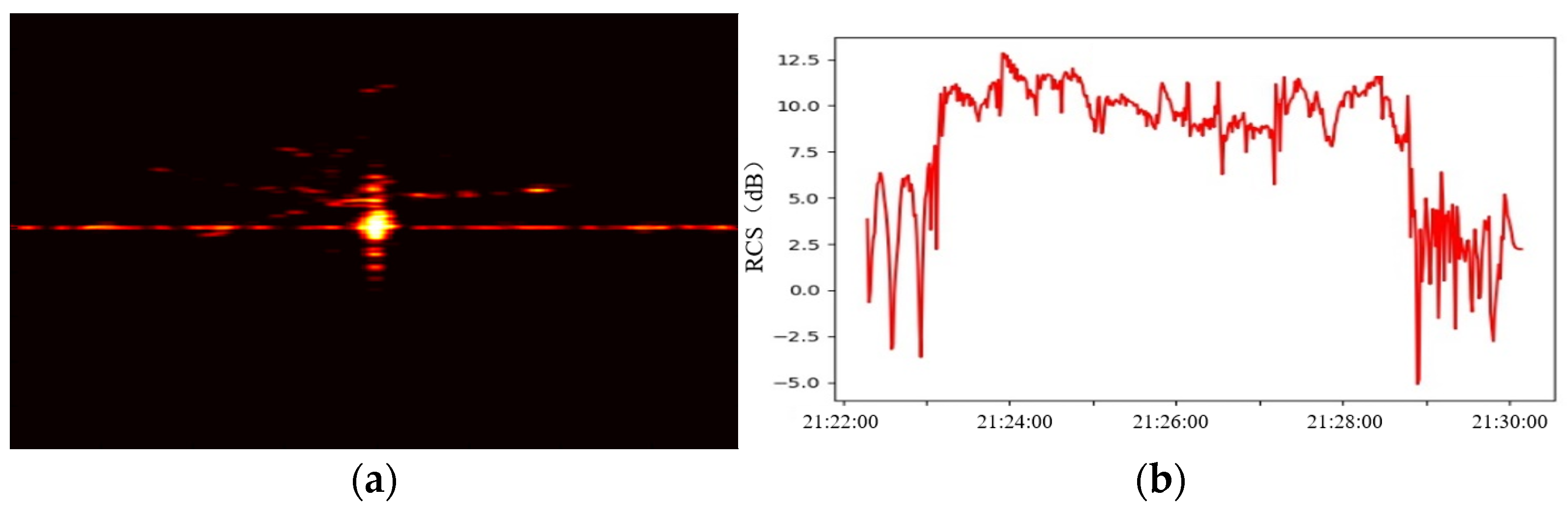
2.1.2. Analysis of Electromagnetic Scattering Characteristics

The full-angle electromagnetic scattering characteristics of the spacecraft carrying the parabolic antenna payload were simulated using the PO/EEC method. Figure 2a provides the full-angle RCS characteristics of a spacecraft with a parabolic antenna payload at the S-band frequency (3 GHz), and Figure 2b presents the variation curves of the target’s RCS with respect to the elevation angle, with the azimuth angle fixed at 0 degrees and 90 degrees, respectively.

From Figure 2, we can see that when the ground-based radar continuously tracked and observed the spacecraft with the parabolic antenna payload, three states were passed through: radar LOS not in the antenna, LOS in the antenna, and LOS not in the antenna. During continuous radar observation, the sequence of RCS measurements shows the step effect. The rising and falling edges of the step effect, which correspond to the change between LOS not in the antenna, LOS in the antenna, and at a particular moment, radar LOS, coincide with the edge of the parabolic antenna. When the radar is in direct view of the spacecraft’s parabolic antenna payload, the RCS of the payload undergoes a step change, which makes the translation compensation in the broadband radar ISAR imaging difficult to complete accurately, resulting in a defocused image, as shown in Figure 3a. At this point, it is difficult to reconstruct the pointing direction orientation of the spacecraft payload using ISAR image information, but the step characteristics of the RCS sequence in the radar’s actual measurement data provide two constraints for the rising edge and the falling edge as shown in Figure 3b, which verifies the correctness of the aforementioned theoretical analysis. Therefore, this paper will utilize the characteristics of the step change in the RCS sequence of the spacecraft carrying a parabolic payload to estimate the orientation of the parabolic antenna payload.

2.2. Mathematical Model of Parabolic Antenna Pointing Estimation

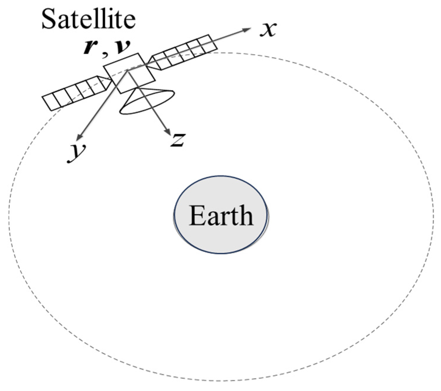
2.2.1. Satellite Orbital Coordinate System

The orientation of the satellite antenna payload is described in the body coordinate system attached to the satellite and the orbital coordinate system. Figure 4 is a schematic diagram of the satellite orbital coordinate system. The satellite orbital plane is the coordinate plane; the Z-axis points from the center of mass of the satellite to the center of the Earth; the X-axis is in the orbit plane, perpendicular to the z-axis, and points in the direction of the satellite’s velocity; and the y-axis is right-handed and orthogonal to the x-axis and z-axis and is parallel to the normal of the orbital plane. The coordinate system rotates in space with the movement of the satellite, and usually, the X, Y, and Z axes are called the roll, pitch, and yaw axes.

By using the parameters of satellite orbital motion $r,v$ (the parameters of satellite orbital motion in the J2000 inertial coordinate system were used in this paper), then the unit vectors of each axis of the orbital coordinate system can be expressed as follows:

$$z={\displaystyle \frac{-r}{\left|r\right|}}$$

(4)

$$y={\displaystyle \frac{v\times r}{\left|v\times r\right|}}$$

(5)

$$x=y\times z$$

(6)

The coordinate transformation matrix from the J2000 inertial coordinate system to the xyz orbital coordinate system can be expressed as follows:

$$R=[\begin{array}{ccc}x& y& z\end{array}]$$

(7)

where $x,y,z$ are column vectors.

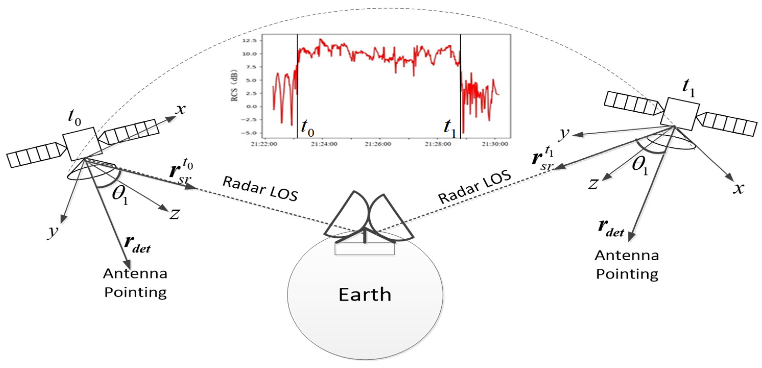
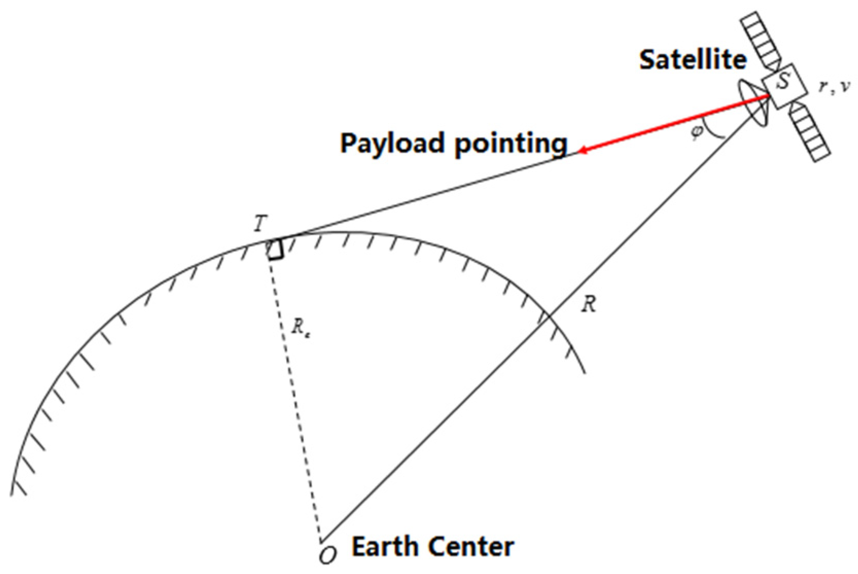
2.2.2. Mathematical Model of Payload Pointing

As shown in Figure 5, it is assumed that the half-cone angle of the parabolic antenna is ${\theta }_p$, and at time $t_0$, the radar detection beam just enters the interior of the parabolic antenna, which is represented on the RCS sequence characteristic curve as the beginning of the step effect and the theoretical angle between the position vector of the satellite to the radar $r_{sr-xyz}^{t_0}$ and antenna pointing $r_{det-xyz}$ in the orbital coordinate system is ${\theta }_p$. Similarly, at time $t_1$, the radar detection beam just leaves the interior of the parabolic antenna, which is represented on the RCS sequence characteristic curve as the end of the step effect and the theoretical angle between the position vector of the satellite to the radar $r_{sr-xyz}^{t_0}$ and antenna pointing $r_{det-xyz}$ in the orbital coordinate system is also ${\theta }_p$.

$$\begin{array}{l}{\phi }_0=<r_{sr-xyz}^{t_0},r_{det-xyz}>=\arccos \left({\displaystyle \frac{r_{sr-xyz}^{t_0}·r_{det-xyz}}{\left|r_{sr-xyz}^{t_0}\right|\left|r_{det-xyz}\right|}}\right)={\theta }_p\\ {\phi }_1=<r_{sr-xyz}^{t_1},r_{det-xyz}>=\arccos \left({\displaystyle \frac{r_{sr-xyz}^{t_1}·r_{det-xyz}}{\left|r_{sr-xyz}^{t_1}\right|\left|r_{det-xyz}\right|}}\right)={\theta }_p\end{array}$$

(8)

We needed to ensure that the satellite’s body coordinate system matched the orbital coordinate system in the initial attitude and that the antenna payload orientation vector was the Z-axis. The attitude of the satellite is described by the Euler angles of rotation of the body coordinate system to the orbital coordinate system; the rotation mode is the internal rotation; and the rotation sequence is 321, d to 0 degrees. Then, the antenna payload pointing vector $r_{det-xyz}$ as shown in Figure 6, it can be expressed as follows:

$$r_{det-xyz}=\left(\begin{array}{ccc}1& 0& 0\\ 0& 1& 0\\ 0& 0& 1\end{array}\right)\left(\begin{array}{ccc}\cos \beta & 0& \sin \beta \\ 0& 1& 0\\ -\sin \beta & 0& \cos \beta \end{array}\right)\left(\begin{array}{ccc}1& 0& 0\\ 0& \cos \alpha & -\sin \alpha \\ 0& \sin \alpha & \cos \alpha \end{array}\right)\left[\begin{array}{l}0\\ 0\\ 1\end{array}\right]=\left[\begin{array}{c}\cos \alpha \sin \beta \\ -\sin \alpha \\ \cos \alpha \cos \beta \end{array}\right]$$

(9)

where $\alpha$ is the roll angle and $\beta$ is the pitch angle.

The satellite-to-station vector under the J2000 coordinate system can be expressed as follows:

$$r_{sr-ECI}^t=r_{r-ECI}^t-r_{s-ECI}^t$$

(10)

where $r_{s-ECI}^t$ is the position vector of the satellite in the J2000 coordinate system and can be obtained through orbital extrapolation and $r_{r-ECI}^t$ is the position vector of the radar station in the J2000 coordinate system and can be converted from the position vector ($r_{r-ECF}$) of the radar station in the geocentric terrestrial reference frame.

$$r_{r-ECI}^t={(PR)}^{\mathrm{T}}{(NR)}^{\mathrm{T}}{(ER)}^{\mathrm{T}}{(EP)}^{\mathrm{T}}{r}_{r-ECF}$$

(11)

where $PR$ is the precession matrix, $NR$ is the nutation matrix, $ER$ is the Earth rotation matrix, and $EP$ is the polar motion matrix.

Then, the satellite-to-station vector in the orbital coordinate system can be expressed as follows:

$$r_{sr-xyz}^t=R^{\mathrm{T}}{r}_{sr-ECI}^t$$

(12)

2.3. Optimization Modeling and Solving

Theoretically, the two unknown quantities of the payload direction can be obtained by solving the two equations in Equation (8) simultaneously. However, considering the measurement information error in the radar and the step effect edge detection time error in the RCS sequence characteristics, this article uses the optimal modeling method for antenna payload inversion.

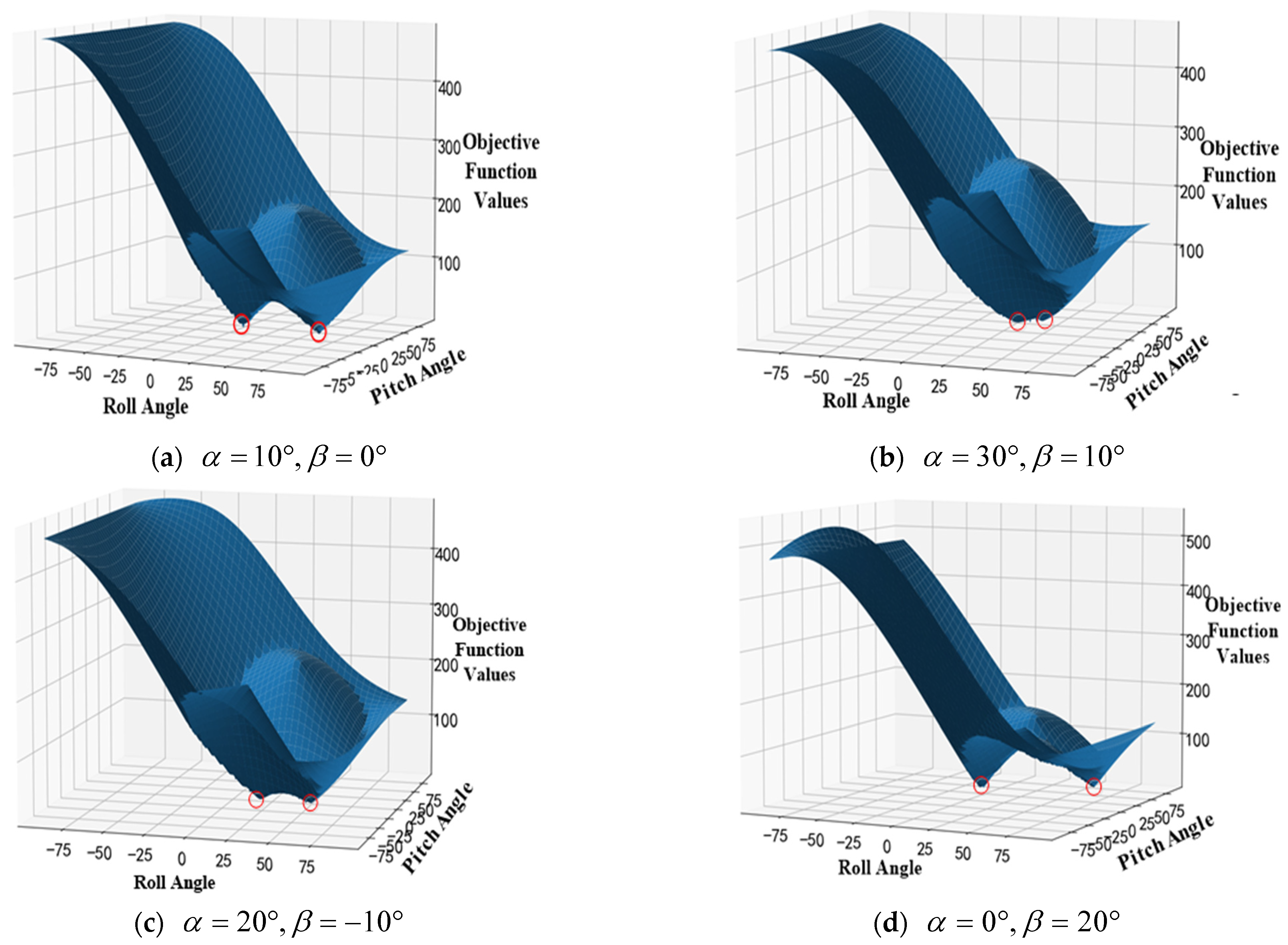
2.3.1. Objective Function

We assumed that the parabolic antenna payload pointing of the spacecraft remained unchanged in the target body system and could be observed by multiple radars within the visible arc segment. Based on the RCS sequence obtained by the radar’s tracking measurement, the rising edge time $t_0$ and the falling edge time $t_1$ of the step effect were detected and extracted, and the angle (${\phi }_i^{m}i=0,1$) between the line of sight from the satellite to the radar and the pointing direction of the parabolic antenna payload was calculated with Equation (8); the objective function can be expressed as follows:

$$J(\alpha ,\beta )={\displaystyle \sum _{m=1}^N{\displaystyle \sum _{i=0}^1{({\phi }_i^m-{\theta }_p)}^2}}$$

(13)

where $N$ represents multiple radars. $i=0,1$ represents the time $t_0$ and $t_1$.

2.3.2. Constraints

Ground Reconnaissance Constraint

The parabolic antenna payload should meet the conditions of ground reconnaissance. Figure 7 shows the geometry of the spacecraft’s parabolic antenna payload for ground reconnaissance.

We assume that the Earth is a sphere with a radius of $R_e$, the position of the spacecraft at time $t$ is $(r,v)$, $T$ is the tangent point of the satellite and the Earth, ${\phi }^m(t)$ represents the angle between the satellite, the tangent point, and the Earth’s center of the mth radar at time $t$; then, the roll angle $\alpha$ and pitch angle $\beta$ of the satellite should be smaller than ${\varphi }^m(t)$:

$$\alpha ,\beta <\min \{{\varphi }^m(t)\}{t}_0^m<t<t_1^m$$

(14)

${\phi }^m(t)$ can be expressed as follows:

$${\varphi }^m(t)=\arccos {\displaystyle \frac{R_e}{R(t)}}$$

(15)

where $R(t)$ is the distance between the satellite and the Earth’s center at time $t$.

RCS Feature Constraint

The radar beam enters the inside of the parabolic antenna at time $t_0$ and exits the inside of the parabolic antenna at time $t_1$. So the angle between the line of sight from the satellite to the radar and the pointing direction of the parabolic antenna payload should be smaller than ${\theta }_p$ and, in theory, between $t_0$ and $t_1$:

$${\phi }^m(t)<{\theta }_p{t}_0^m<t<t_1^m$$

(16)

Side-Swing Ability Constraint

Let the maximum side-swing angle of the parabolic antenna be ${\theta }_f$; then, the roll angle $\alpha$ and pitch angle $\beta$ of the satellite should be smaller than ${\theta }_f$:

$$\alpha ,\beta \le {\theta }_f$$

(17)

2.3.3. Optimization Model

This paper proposes an optimization algorithm for the inversion of the parabolic antenna payload pointing. The angle error is optimized under the conditions of satisfying the ground reconnaissance constraint, the RCS feature constraint, and the side-swing ability constraint. An optimization model as follows can be established under the multi-station observation conditions.

$$\begin{array}{l}\min J(\alpha ,\beta )={\displaystyle \sum _{m=1}^N{\displaystyle \sum _{i=0}^1{({\phi }_i^m-{\theta }_p)}^2}}\\ s.t.\{\begin{array}{l}\alpha ,\beta \le {\theta }_f\\ {\phi }^m(t)<{\theta }_p\hspace{1em}{t}_0^m<t<t_1^m\\ \alpha ,\beta <\min \left\{{\varphi }^m\right(t\left)\right\}\hspace{1em}{t}_0^m\le t\le t_1^m\end{array}\end{array}$$

(18)

For single-station measurement, the optimization mode can be simplified as follows:

$$\begin{array}{l}\min J(\alpha ,\beta )={\displaystyle \sum _{i=0}^1{({\phi }^i-{\theta }_p)}^2}\\ s.t.\{\begin{array}{l}\alpha ,\beta \le {\theta }_f\\ \phi (t)<{\theta }_p\hspace{1em}{t}_0<t<t_1\\ \alpha ,\beta <\min \left\{\varphi \right(t\left)\right\}\hspace{1em}{t}_0\le t\le t_1\end{array}\end{array}$$

(19)

2.3.4. Modified Particle Swarm Optimization

In the previous text, an objective optimization function for payload orientation inversion was established. This paper uses the optimization solution algorithm to find the optimal solution within the solution space of payload orientation to determine the payload’s pointing direction. The HPSO is an improved version of the PSO was used in this paper.

To control the convergence speed of the process, the quantum behavior operator is introduced to strengthen the particles’ convergence ability. The particles update their positions according to the following equation:

$$v_{id}^{k+1}=C_v\times v_{id}^k+C_x\times (pbes{t}_{id}^k-x_{id}^k)+C_g\times (gBes{t}_d^k-x_{id}^k)$$

(20)

where $C_v$ and $C_x$ are phase coefficients related to the particle velocity $v_{id}^k$ and the particle position $x_{id}^k$, respectively; $C_g$ is phase coefficient related to the best global position of the swarm $gBes{t}_n^k$.

Because the PSO system is a kind of quantum behavior, the position and velocity of particles in quantum space cannot be determined at the same time. The particle motion state determined by the wave function, the updated position of the particle can be determined by the following equation:

$$x_{in}^{k+1}=p_{in}^k\pm \alpha \cdot \left|mBes{t}_n^k-x_{in}^k\right|\cdot \ln \left({\displaystyle \frac{1}{u_{in}^k}}\right)$$

(21)

where $\alpha$ is the compress–expand factor, $mBes{t}_n^k$ is the current mean best position of the swarm at time step $k$ in the $n$th-dimensional search space, and $u_{in}^k$ is a random number within the range [0, 1].

The flow chart of the HPSO algorithm is provided in Figure 8, and the calculation process is as follows:

The first step: Randomly generate the particle swarm with swarm size $N$, particle dimension $D$, the maximum number of iterations $MaxIter$, convergence threshold $Eps$, and mutation probability $P_m$, and initialize the iteration number $k=0$. In this study, the number of particles was set to 30, and the maximum number of iterations was 500.

The second step: the fitness values of all particles are evaluated using Equation (18) or (19).

The third step: the positions and velocities of all particles are evaluated using Equations (20) and (21).

The fourth step: update the values, and then calculate the mean fitness value and the best fitness value using the following formulas:

$$\begin{array}{l}{F}_{ave}={\displaystyle \sum _{m=1}^{N}Fitnes{s}_m/N}\\ F_{opt}=gBes{t}^k\end{array}$$

(22)

where $Fitnes{s}_m$ is the fitness value of particle $m$.

The fifth step: According to the mutation probability $P_m/D$, the particle dimension is randomly selected. Then, the $d\mathrm{th}$ dimension position of the particle is mutated as follows:

$$x_{id}=x_{id}+k_3\cdot C_{id}$$

(23)

where $C_{id}$ is the normal cloud parameter.

The sixth step: Check the calculation termination conditions. If the convergence threshold $Eps$ or the maximum number of iterations $MaxIter$ is reached, the calculation ends. Otherwise, return to the second step.

3. Results

3.1. Simulation Verification

The subject of the simulation experiment is Israel’s TECSAR-2 synthetic aperture radar (SAR) Earth observation satellite, whose SAR antenna is a deployable umbrella-shaped parabolic antenna. The simulation parameter settings are shown in

Table 1. Simulation parameter settings.

Time Setting (UTC)	Start Time:	2022-4-2 8:32:00
	End Time:	2022-4-2 8:40:00
Satellite Orbital Parameters	Inclination:	140.9213
	RA of the Ascending Node:	208.9937
	Eccentricity:	0.0001218
	Perigee Argument:	162.7295
	Mean Anomaly:	1.2422
	Mean angular velocity:	15.16888613
Radar Station Position	Longitude:	110
	Latitude:	32
	Height:	0.1

, where the orbital parameters are derived from the TLE elements announced on the same day.

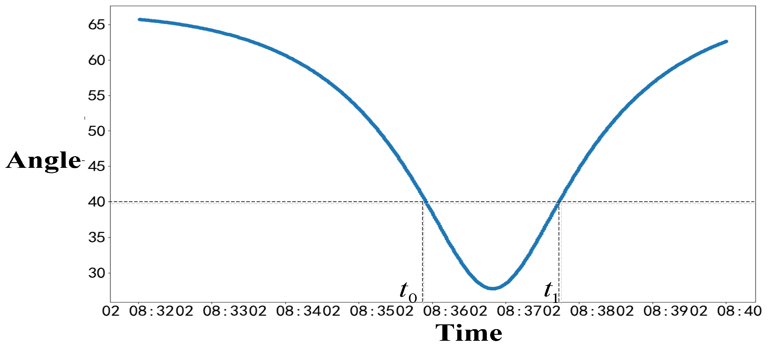
3.1.1. Single-Station Measurement

Let the semi-cone angle of the parabolic antenna be ${\theta }_p=40°$, the pointing angle of the parabolic antenna payload be $\alpha =-10°,\beta =0°$, and the curve of the angle between the position vector of the satellite to the radar and antenna pointing in the orbital coordinate system with time is shown in Figure 9.

Find the time points corresponding to the angle of $40°$ in Figure 9, which are the corresponding $t_0$ and $t_1$ moments; the obtained $t_0$ moment is 8:35:54; and the $t_1$ moment is 8:37:44.

Set the initial population size to 30, with 500 iterations and a side-swing angle of 90 degrees for the satellite. By using the HPSO algorithm for calculation, two optimal solutions for the pointing of the antenna payload could be obtained through multiple calculations, as shown in

Table 2. Single-station measurement simulation results.

Setting Value	Inversion Value
$\alpha =-10°,\beta =0°$	Value 1: $\alpha =-10.33°,\beta =0.04°$
	Value 2: $\alpha =-63.89°,\beta =-2.31°$

, and the solution was not unique.

To verify the number of possible solutions under the single-station measurement condition, the variation relationship of the objective function values under different satellite pointing situations in the solution space is shown in Figure 10.

From Figure 10, it can be seen that under the single-station measurement condition, when the solution space range is within 90 degrees, there are two locally optimal solutions for the satellite antenna payload orientation as shown in the red circle in Figure 10. The reason why single-station measurements cannot obtain a unique solution is due to the symmetry of the parabolic antenna. For instance, consider an extreme case where the satellite passes directly overhead of the measurement station. In this scenario, whether the satellite’s parabolic payload is tilted 10 degrees to the left or to the right, the radar measurements of the RCS sequence will yield the same starting and ending points for the step effect. Consequently, a single-station measurement cannot determine a unique solution. At this time, the unique load indication cannot be obtained. It can be seen from Figure 10 that when the solution space range is within 45 degrees, only a locally optimal solution remains, and the unique load orientation can be obtained.

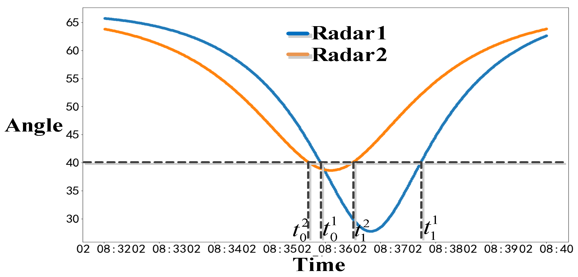
3.1.2. Multi-Station Measurement

Based on a single-station measurement, an additional measurement station (longitude: 112, latitude: 33, altitude: 0.1) was considered in keeping with the other simulation parameters, the angular curves between the satellite’s position vector to the radars and the inward-facing antenna were maintained using the orbital coordinate system of time shown in Figure 11.

Find the time points corresponding to the angle of $40°$ in Figure 11 through multiple calculations using the HPSO algorithm, and the only values obtained are $\alpha =-10.04°,\beta =-0.11°$.

To verify the uniqueness of the solution under the multi-station measurement condition, the varying relationship of the objective function values under different satellite pointing situations in the solution space is shown in Figure 12.

It can be seen from Figure 12 that due to the increased limitations in multi-station measurements, there is only a locally optimal solution when the solution space area is 90 degrees, and a unique solution can be inverted as shown in the red circle in Figure 12.

3.1.3. Comparison of Single-Station and Multi-Station Results

The comparison of payload pointing inversion results between single-station and multi-station measurements is shown in

Table 3. Comparison of single-station and multi-station.

Setting Value	Inversion Value Single-Station	Inversion Value Multi-Station
$\alpha =-10°,\beta =0°$	1:$\alpha =-10.33°,\beta =0.04°$	$\alpha =-10.13°,\beta =0.04°$
	2:$\alpha =-63.89°,\beta =-2.31°$
$\alpha =0,\beta =10°$	1:$\alpha =-0.31°,\beta =11.22°$	$\alpha =0.53°,\beta =10.82°$
	2:$\alpha =-72.34°,\beta =34.65°$
$\alpha =0°,\beta =0°$	1:$\alpha =0.52°,\beta =1.58°$	$\alpha =0.33°,\beta =1.21°$
	2:$\alpha =-75.61°,\beta =-6.02°$
$\alpha =-10°,\beta =-20°$	1:$\alpha =-10.54°,\beta =-21.23°$	$\alpha =-10.13°,\beta =-18.57°$
	2:$\alpha =-53.26°,\beta =-40.99°$

.

It can be seen from Table 3 that single-station measurements find it difficult to invert a unique solution, while multi-station measurements can determine a unique solution, and the inversion accuracy is also superior to that of single-station measurements.

3.2. Precision Analysis

3.2.1. Errors Caused by the Accuracy of Time Extraction

The antenna payload orientation estimation algorithm proposed in this paper is based on the $t_0$ and $t_1$ time values of RCS sequence feature extraction. Different time values lead to different reversal antenna payload angles. By artificially setting the error values of the $t_0$ and $t_1$ moment, the inverse calculation of the antenna payload orientation is performed to obtain the angular error curve, as shown in Figure 13.

From Figure 13, it can be seen that the payload orientation estimation error is less than 0.25 degrees when the timing error is within 5 s. The simulation results show that since the algorithm fully utilizes all measurement information between $t_0$ and $t_1$, it is not very time-sensitive and has good robustness.

3.2.2. Errors Caused by the Optimization Algorithm

Currently, not all optimization algorithms can completely overcome local optima. In order to analyze the error in estimating the payload orientation caused by the optimization algorithm, this paper selected four influencing factors: satellite orbital altitude, roll angle, pitch angle, and dual station layout position, and selected three levels for each factor. The $L_9(3^4)$ orthogonal test table was developed for simulation analysis.

From

Table 4. Payload pointing estimation error orthogonal experimental analysis.

Number	Orbital Altitude/km	Roll Angle	Pitch Angle	Station Layout Position	Inversion Result	Error
1	500	10	−25	Lon1 = Lon2 Lat1 $\ne$ Lat2	$\alpha =12.08°,\beta =-25.03°$	$2.08°$
2	500	25	0	Lon1 $\ne$ Lon2 Lat1 = Lat2	$\alpha =24.08°,\beta =-2.08°$	$2.27°$
3	500	40	25	Lon1 $\ne$ Lon2 Lat1 $\ne$ Lat2	$\alpha =41.35°,\beta =25.18°$	$1.39°$
4	750	10	0	Lon1 $\ne$ Lon2 Lat1 $\ne$ Lat2	$\alpha =11.04°,\beta =0.07°$	$1.08°$
5	750	25	25	Lon1 = Lon2 Lat1 $\ne$ Lat2	$\alpha =23.62°,\beta =24.92°$	$1.39°$
6	750	40	−25	Lon1 $\ne$ Lon2 Lat1 = Lat2	$\alpha =42.40°,\beta =-25.27°$	$2.48°$
7	1000	10	25	Lon1 $\ne$ Lon2 Lat1 = Lat2	$\alpha =8.47°,\beta =24.97°$	$1.53°$
8	1000	25	−25	Lon1 $\ne$ Lon2 Lat1 $\ne$ Lat2	$\alpha =22.91°,\beta =-25.03°$	$2.85°$
9	1000	40	0	Lon1 = Lon2 Lat1 $\ne$ Lat2	$\alpha =38.98°,\beta =-0.2°$	$1.2°$

, it can be seen that the error in estimating payload orientation caused by the optimization algorithm did not exceed three degrees; the maximum error was 2.85 degrees; and the mean error was 1.63 degrees, which shows relatively good estimation accuracy.

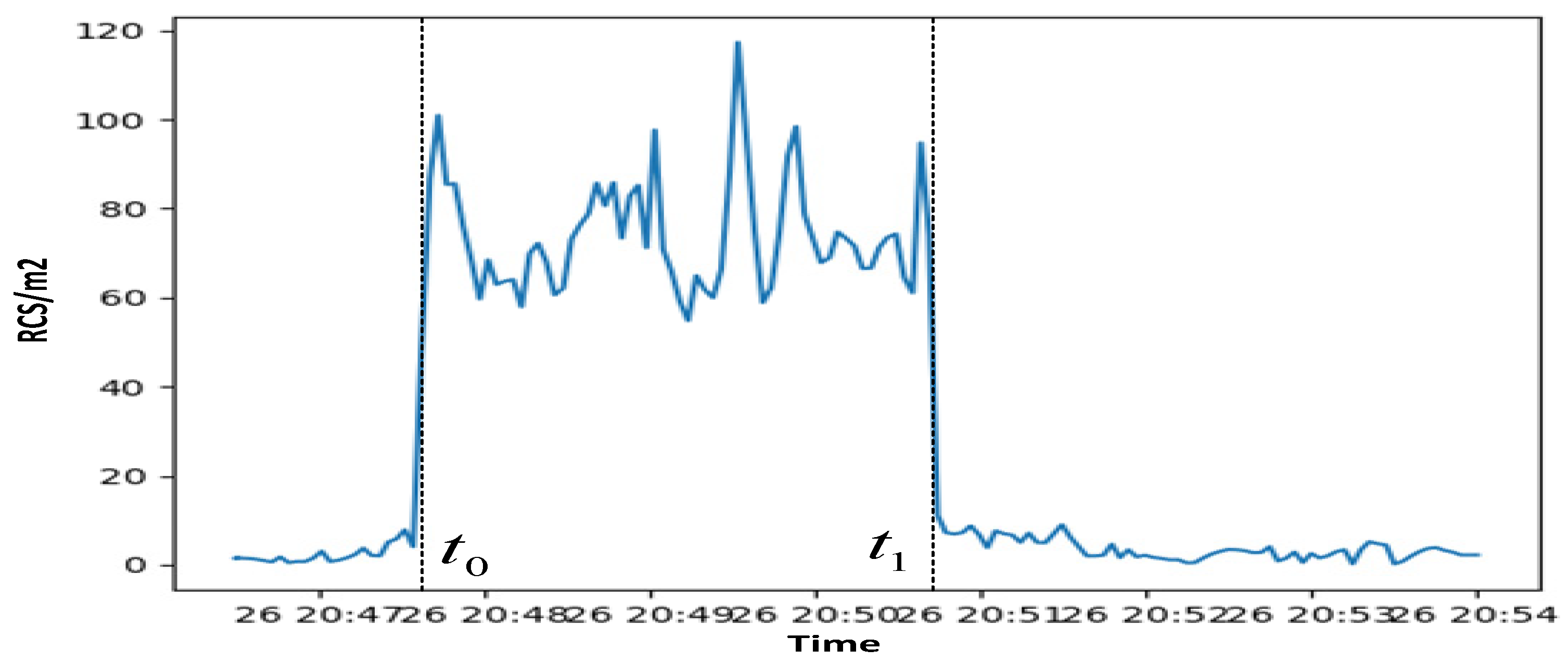
3.3. Application of Empirical Data

The RCS sequence of a spacecraft with a parabolic antenna payload, as observed by radars passing over the ground station, is shown in Figure 14.

We extracted the moments of $t_0$ and $t_1$ to be 20:47:33 and 20:50:44. We input the satellite orbital elements, the location of the tracking station, the semi-conical angle of the parabolic antenna ${\theta }_p=50°$, and the $t_0$ and $t_1$, moments, respectively. Considering the actual yaw capability of the satellite’s side-swing angle within the range of 45 degrees, through multiple inversions, it is determined that the pointing direction of the parabolic antenna payload is $\alpha =2.7°,\beta =-6.5°$ as shown in

Table 5. Empirical data inversion results.

System Input	System Output
Satellite orbital elements	$\alpha =2.7°$
Location of the tracking station
$t_0$: 20:47:33
$t_1$: 20:50:44	$\beta =-6.5°$
Semi-conical angle of the parabolic antenna: ${\theta }_p=50°$
Max side-swing angle of the antenna: ${\theta }_f=45°$

.

To verify the adaptability of the algorithm in this paper to different types of parabolic antenna loads, multi-arc RCS measurement data were collected from two on-orbit spacecraft equipped with parabolic antenna loads (Haiwangxing 01 and TECSAR-2). Arcs with step effects were identified, and the payload pointing was inverted using the algorithm presented in this paper, as shown in

Table 6. Inverse results of different satellite payload pointing.

Satellite	Arc Segment	Measurement Time (UTC)	${\mathit{t}}_0$$\mathbf{and} {\mathit{t}}_1$ Moments	Inversion Result
Haiwangxing 01	1	Start Time: 2024-03-24 04:35:00	$t_0$ 04:36:05	$\alpha =16.2°$ $\beta =9.3°$
		End Time: 2024-03-24 04:40:10	$t_1$ 04:39:10
	2	Start Time: 2024-10-11 03:22:00	$t_0$ 03:23:04	$\alpha =-19.4°$ $\beta =4.6°$
		End Time: 2024-10-11 03:25:10	$t_1$ 03:24:32
TECSAR-2	1	Start Time: 2022-04-28 05:10:00	$t_0$ 05:11:08	$\alpha =16.2°$ $\beta =8.2°$
		End Time: 2022-04-28 05:16:10	$t_1$ 05:15:06
	2	Start Time: 2022-05-26 20:47:00	$t_0$ 20:47:33	$\alpha =2.7°$ $\beta =-6.5°$
		End Time: 2022-05-26 20:54:00	$t_1$ 20:50:44

.

It can be seen from Table 6 that if a real RCS sequence of the target with a step effect can be obtained, the pointing of the parabolic antenna load can be inverted based on the algorithm in this paper, indicating that the algorithm has good adaptability.

4. Conclusions

This article proposes an estimation method for the orientation of a spacecraft’s parabolic antenna payload based on the step effect of RCS sequences. By exploiting the step effect on the target RCS sequence caused by the line-of-sight change between the spacecraft parabolic antenna payload and the ground-based radar during their mutual line of sight, a computational model for the pointing direction of the antenna payload is founded on this basis. The method allows for the estimation of the orientation of the parabolic antenna payload, and both simulation and empirical measurement results have confirmed the effectiveness and robustness of this algorithm.

References

1. Lin, H.-Y.; Zhao, C.-Y. An estimation of Envisat’s rotational state accounting for the precession of its rotational axis caused by gravity gradient torque. Adv. Space Res. 2018, 61, 182–188. [Google Scholar] [CrossRef]
2. Zhong, W.J.; Wang, J.S.; Ji, W.J.; Lei, X.; Zhou, X.W. The attitude estimation of three-axis stabilized satellites using hybrid particle swarm optimization combined with radar cross section precise prediction. Inst. Mech. Eng. Part G J. Aerosp. Eng. 2015, 31, 222–224. [Google Scholar] [CrossRef]
3. Lyu, J.T.; Zhong, W.J.; Liu, H.; Geng, Y.; Ben, D. Novel Approach to Determine Spinning Satellites’ Attitude by RCS Measurements. J. Aerosp. Eng. 2021, 34, 04021023. [Google Scholar] [CrossRef]
4. D’Amico, S.; Benn, M.; Jørgensen, J.L. Pose estimation of an uncooperative spacecraft from actual space imagery. Int. J. Space Sci. Eng. 2014, 1, 171–189. [Google Scholar]
5. Sommer, S.; Rosebrock, J.; Cerutti-Maori, D.; Leushacke, L. Temporal analysis of ENVISAT’s rotational motion. In Proceedings of the 7th European Conference on Space Debris, Darmstadt, Germany, 18–21 April 2017; pp. 18–21. [Google Scholar]
6. Lemmens, S.; Krag, H.; Rosebrock, J. Radar mappings for attitude analysis of objects in orbit. In Proceedings of the 6th European Conference on Space Debris, Darmstadt, Germany, 22–25 April 2013; pp. 20–24. [Google Scholar]
7. Lemmens, S.; Krag, H. Sensitivity of automated attitude determination form ISAR radar mappings. In Proceedings of the Advanced Maui Optical and Space Surveillance Technologies Conference (AMOS), Maui, HI, USA, 10–13 September 2013. [Google Scholar]
8. Wang, Q.Y.; Wang, Z.Y. Position and pose measurement of spacecraft based on monocular vision. J. Appl. Opt. 2017, 38, 250–255. [Google Scholar] [CrossRef]
9. Zhou, Y.; Zhang, L.; Cao, Y.; Wu, Z. Attitude estimation and geometry reconstruction of satellite targets based on ISAR image sequence interpretation. IEEE Trans. Aerosp. Electron. Syst. 2018, 55, 1698–1711. [Google Scholar] [CrossRef]
10. Zhou, Y.; Zhang, L.; Cao, Y. Dynamic Estimation of Spin Spacecraft Based on Multiple-Station ISAR Images. IEEE Trans. Geosci. Remote Sens. 2019, 58, 2977–2989. [Google Scholar] [CrossRef]
11. Avilés, M.; Margarit, G.; Canetri, M.; Lemmens, S. Automated attitude estimation from ISAR images. In Proceedings of the 7th European Conference on Space Debris, Darmstadt, Germany, 18–21 April 2017; pp. 1–13. [Google Scholar]
12. Xie, P.; Zhang, L.; Du, C.; Wang, X.; Zhong, W. Space Target Attitude Estimation from ISAR Image Sequences with Key Point Extraction Network. IEEE Signal Process. Lett. 2021, 28, 1041–1045. [Google Scholar] [CrossRef]
13. Zhou, Y.; Zhang, L.; Cao, Y.; Huang, Y. Optical-and-radar image fusion for dynamic estimation of spin satellites. IIEEE Trans. Image Process. 2019, 29, 2963–2976. [Google Scholar] [CrossRef] [PubMed]
14. Suwa, K.; Wakayama, T.; Iwamoto, M. Three-dimensional target geometry and target motion estimation method using multi-static ISAR movies and its performance. IEEE Trans. Geosci. Remote Sens. 2011, 49, 2361–2373. [Google Scholar] [CrossRef]
15. Zhou, Y.; Zhang, L.; Cao, Y. Attitude estimation for space targets by exploiting the quadratic phase coefficients of inverse synthetic aperture radar imagery. IEEE Trans. Geosci. Remote Sens. 2019, 57, 3858–3872. [Google Scholar] [CrossRef]
16. Zhou, Y.; Zhang, L.; Wei, S.; Cao, Y. Dynamic Analysis of Spin Satellites Through the Quadratic Phase Estimation in Multiple-Station Radar Images. IEEE Trans. Comput. Imaging 2020, 6, 894–907. [Google Scholar] [CrossRef]
17. Lefferts, E.; Markley, F.; Shuster, M.D. Kalman filtering for spacecraft attitude estimation. J. Guid. Control. Dyn. 1982, 5, 417–429. [Google Scholar] [CrossRef]
18. Virgili, B.B.; Lemmens, S.; Krag, H. Investigation on Envisat attitude motion. In Proceedings of the e. Deorbit Workshop, Noordwijk, The Netherlands, 6 May 2014. [Google Scholar]
19. Huo, C.Y.; Yin, H.C.; Xing, X.Y.; Liang, M. Attitude direction estimation for space target antenna load based on radar image features. Chin. J. Radio Sci. 2019, 34, 45–51. [Google Scholar]
20. Zhang, Y.; Yang, X.; Jiang, X.R. Attitude direction estimation of space target parabolic antenna loads using sequential terahertz ISAR images. J. Infrared Millim. Waves 2021, 40, 496–507. [Google Scholar]
Figure 1. Geometric structure diagram of the ground-based radar observing the spacecraft.
Remotesensing 16 04259 g001
Figure 2. Schematic diagram of the RCS variation trend of a spacecraft at full angles and with a fixed azimuth angle as the elevation angle changes. (a) Full-angle RCS characteristics of the target at the S-band. (b) Variation curve of the target’s RCS with the pitch angle.
Remotesensing 16 04259 g002
Figure 3. Schematic diagram of ISAR image defocus and measured data of the RCS sequence with step characteristics. (a) ISAR image defocus. (b) Measured data RCS sequence with step characteristics.
Remotesensing 16 04259 g003
Figure 4. Schematic diagram of the satellite orbital coordinate system.
Remotesensing 16 04259 g004
Figure 5. Radar observation spacecraft with parabolic antenna payload.
Remotesensing 16 04259 g005
Figure 6. Schematic diagram of antenna payload pointing vector.
Remotesensing 16 04259 g006
Figure 7. Geometry of the spacecraft parabolic antenna payload for ground reconnaissance.
Remotesensing 16 04259 g007
Figure 8. Flowchart of HPSO algorithm.
Remotesensing 16 04259 g008
Figure 9. The curve of the angle between the position vector of the satellite to the radar and antenna pointing.
Remotesensing 16 04259 g009
Figure 10. Objective function values under single-station measurement.
Remotesensing 16 04259 g010
Figure 11. The curves of the angle between the position vector of the satellite to the radars and antenna pointing.
Remotesensing 16 04259 g011
Figure 12. Objective function values under multi-station measurement.
Remotesensing 16 04259 g012
Figure 13. Angle error caused by time error.
Remotesensing 16 04259 g013
Figure 14. Empirically measure RCS sequence.
Remotesensing 16 04259 g014