An Assessment of the Seasonal Uncertainty of Microwave L-Band Satellite Soil Moisture Products in Jiangsu Province, China

Abstract

Accurate surface soil moisture (SM) data are crucial for agricultural management in Jiangsu Province, one of the major agricultural regions in China. However, the seasonal performance of different SM products in Jiangsu is still unknown. To address this, this study aims to evaluate the applicability of four L-band microwave remotely sensed SM products, namely, the Soil Moisture Active Passive Single-Channel Algorithm at Vertical Polarization Level 3 (SMAP SCA-V L3, hereafter SMAP-L3), SMOS-SMAP-INRAE-BORDEAUX (SMOSMAP-IB), Soil Moisture and Ocean Salinity in version IC (SMOS-IC), and SMAP-INRAE-BORDEAUX (SMAP-IB) in Jiangsu at the seasonal scale. In addition, the effects of dynamic environmental variables such as the leaf vegetation index (LAI), mean surface soil temperature (MSST), and mean surface soil wetness (MSSM) on the performance of the above products are investigated. The results indicate that all four SM products exhibit significant seasonal differences when evaluated against in situ observations between 2016 and 2022, with most products achieving their highest correlation (R) and unbiased root-mean-square difference (ubRMSD) scores during the autumn. Conversely, their performance significantly deteriorates in the summer, with ubRMSD values exceeding 0.06 m³/m³. SMOS-IC generally achieves better R values across all seasons but has limited temporal availability, while SMAP-IB typically has the lowest ubRMSD values, even reaching 0.03 m³/m³ during morning observation in the winter. Additionally, the sensitivity of different products’ skill metrics to environmental factors varies across seasons. For ubRMSD, SMAP-L3 shows a general increase with LAI across all four seasons, while SMAP-IB exhibits a notable increase as the soil becomes wetter in the summer. Conversely, wet conditions notably reduce the R values during autumn for most products. These findings are expected to offer valuable insights for the appropriate selection of products and the enhancement of SM retrieval algorithms.

1. Introduction

Surface soil moisture (SM) determines the photosynthesis and transpiration of vegetation and is a key variable affecting crop growth, land–atmosphere water and heat exchange, as well as the water cycle process [1,2]. Accurate, long-term monitoring and rapid repetitive recording of SM dynamics over large regions are essential for effective agricultural drought surveillance [3]. Furthermore, such monitoring helps in understanding the relationship between water and carbon cycles [4,5,6].

Ground stations provide precise SM measurements but suffer from limited spatial coverage, which restricts their capacity to capture the large spatio-temporal variations of SM, particularly across expansive agricultural landscapes [7]. In contrast, optical remote sensing offers extensive coverage but is susceptible to being affected by cloud cover and nighttime conditions, limiting its continuity and reliability for SM monitoring. In comparison, microwave remote sensing can penetrate through clouds, rain, and snow, as well as the atmosphere, and is not affected by weather conditions such as lighting. Moreover, microwave remote sensing at L-band (1.4 GHz), sensitive to the soil dielectric constant, with high revisit frequencies and immunity to adverse weather conditions, has emerged as a promising tool for monitoring SM [8,9]. This technology, with its all-weather high-coverage capabilities and enhanced penetration capability through vegetation, is increasingly being applied in current SM estimation and application studies [8,10,11,12].

Over the past few decades, numerous satellite platforms equipped with passive/active microwave sensors operating at different frequencies have been successfully launched. The Soil Moisture Active Passive (SMAP) [13] and Soil Moisture and Ocean Salinity (SMOS) [14] missions are in-orbit L-band initiatives dedicated to SM estimation. Both space missions are regarded as highly effective for SM monitoring, owing to their stronger ability to penetrate vegetation in the L-band compared to the X- or C-band [15,16]. SM products from these missions are offered both as standalone datasets and as integrated series, including the long-term series developed by ESA’s Climate Change Initiative (CCI) SM project [15,17], as well as the SMOS-SMAP-INRAE-BORDEAUX (SMOSMAP-IB) product, which fused brightness temperature observations from SMOS and SMAP [18]. Performance assessment of satellite-derived SM retrievals is critical for enhancing the algorithms of these products and exploring their applications in climate, hydrology, and disaster management, including flood and drought responses [2,10,19,20,21,22,23,24]. Assessment studies on SM have so far been carried out extensively across China or in specific subregions such as watersheds like the Heihe River [25] and the Luanhe River [19]. Moreover, such assessment is particularly vital for cropland areas, as accurate SM data directly influence agricultural water management practices, including the development and implementation of irrigation strategies [26]. However, due to the limited availability of ground observations, few investigations have been conducted on cropland in Jiangsu Province, a key agricultural province in China.

Jiangsu Province, covering an area of 107,200 km², has approximately 40% of its land dedicated to agriculture and follows a seasonal cropping cycle. Specifically, rice is sown in the spring and harvested in the autumn, while wheat is planted in the autumn and harvested in the summer. These crops, with their distinct growth stages, require varied SM levels throughout the seasons. Therefore, evaluating the performance of satellite SM retrievals at the seasonal scale is crucial for optimizing agricultural practices in the region [21]. Although the recent assessment by Fan et al. [27] provides valuable insights into the performance of various satellite products in Jiangsu, it does not address the seasonal variation in the performance of different satellite SM products. Furthermore, SM retrieval algorithms are rapidly evolving, with continuous improvements and revisions being made [28,29]. Innovations and recalibrations are regularly integrated, leading to enhanced and optimized algorithm parameters [8,30]. Consequently, newly released SM products and updated versions have not yet undergone comprehensive evaluation and intercomparison. One of these new products is the SMOSMAP-IB SM product, which has so far been assessed primarily using in situ observations from the International Soil Moisture Networks (ISMN) located mainly in the United States and Europe [18] and has not been systematically validated in China.

In this context, and to fill the aforementioned gaps, this study aims to assess the performance of multi-source microwave remotely sensed SM products at the seasonal scale, utilizing the most recent long-term in situ observation data from 2016 to 2022. Additionally, the retrieval capabilities of these SM inversion algorithms are investigated under a variety of environmental conditions characterized by distinct seasonal variations. Three environmental dynamics (leaf area index (LAI), mean surface soil temperature (MSST), and mean surface soil wetness (MSSM)) are considered in the analyses to identify factors contributing to discrepancies relative to in situ measurements [10]. It should be noted that our ground observations cover multiple land cover types, not just cropland, enabling a more comprehensive analysis of the effects of different external factors, especially varying LAI levels. By examining how these variables affect microwave satellite SM products, we can gain a deeper understanding of their accuracy and provide a research basis for developers to refine and enhance SM retrieval algorithms [31].

The structure of this paper is organized as follows: Section 2 provides a brief introduction to the datasets, while Section 3 details the methodology. Results are presented in Section 4, followed by discussions in Section 5. Lastly, Section 6 summarizes the conclusions.

2. Datasets

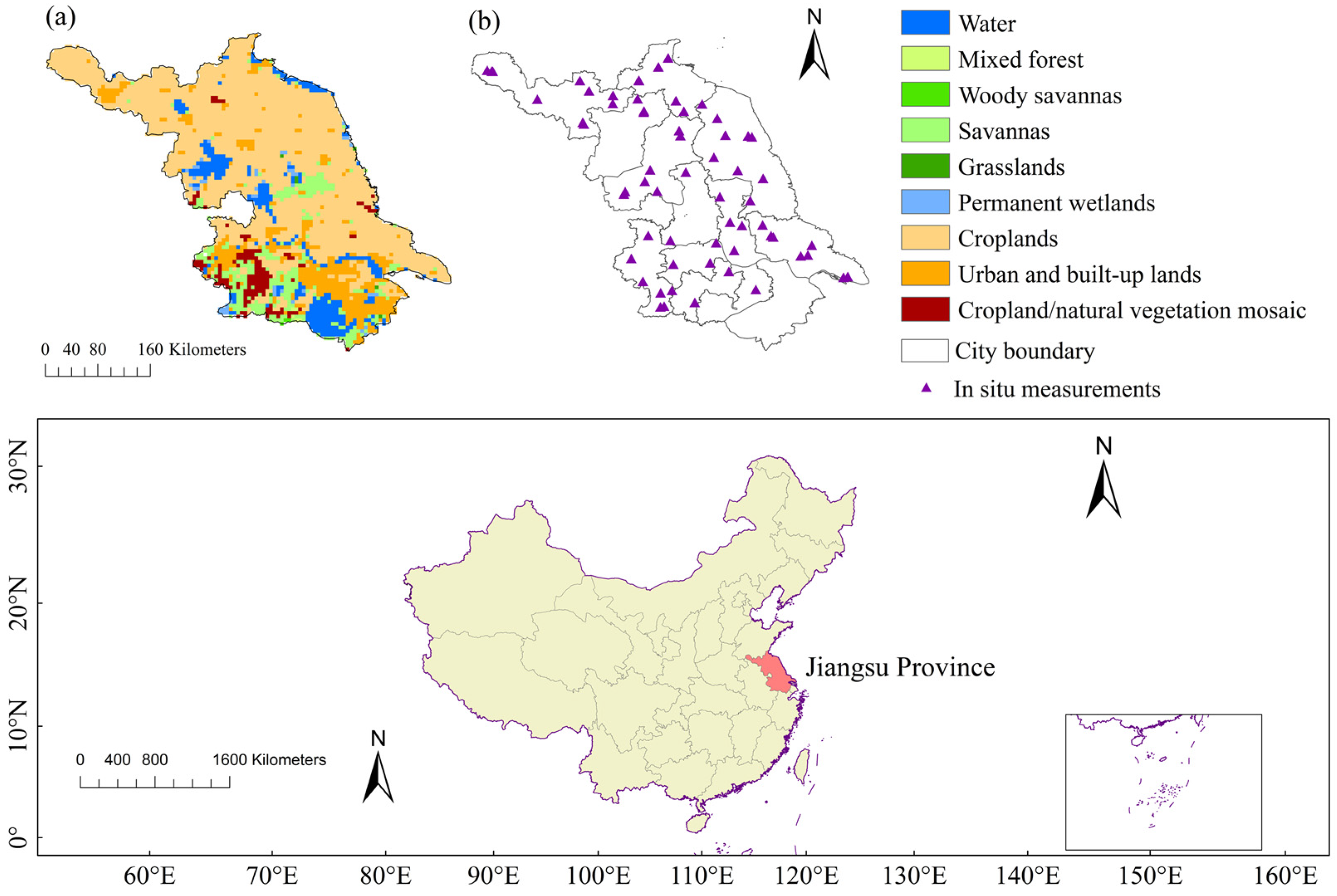
2.1. Study Area and In Situ Measurements

Jiangsu Province, located in the eastern coastal region of China, is a significant part of the Yangtze River Delta urban agglomeration. Jiangsu Province is predominantly characterized by plains, with the highest proportion of plain area among all provinces. It boasts a multitude of rivers and is dominated by agricultural land, with the southern part of Jiangsu having a larger urban area than the northern part (Figure 1a). The climate in Jiangsu transitions from temperate to subtropical, with rainfall primarily concentrated in the summer. Due to the interplay of land and sea distribution, atmospheric circulation, and seasonal precipitation patterns, Jiangsu is prone to both droughts and floods.

In situ observations are collected from automated monitoring instruments deployed by the Jiangsu Provincial Meteorological Bureau, based on the Frequency Domain Reflection principle to measure soil volumetric water content. Sensor calibration, essential for data accuracy, included both laboratory and field calibration. Observations are conducted at depths ranging from 0 cm to 100 cm, including specific intervals of every 10 cm in the first 60 cm, then at 70–80 cm and 90–100 cm, with a temporal resolution of 1 h. Here, only in situ SM data observed in the 0–10 cm layer from 62 stations (Figure 1b) after quality control covering a long period of 2016–2022 are used for evaluation purposes.

2.2. Satellite SM Products Datasets

Four L-band passive microwave satellite SM datasets spanning from 1 January 2016 to 31 December 2022 are employed in this study. The reason for choosing only L-band products is that this band has a stronger penetration capability compared to X- and C-band, and its SM products have been found to be more promising than the other two bands [8,19]. These datasets include SMAP-L3, SMAP-IB, SMOS-IC, and SMOSMAP-IB, as outlined in Table 1.

(1) SMOS-IC version 2: The European Space Agency (ESA) launched SMOS in 2009 as the first polar-orbiting L-Band radiometer, offering a spatial resolution of around 43 km and a revisit time of three days. Since its launch, several datasets have been generated based on SMOS multi-angle observations, including SMOS Level 2, SMOS Level 3, and SMOS-IC, all of which utilize the L-band Microwave Emission of the Biosphere (L-MEB) model in their inversion process. In this study, the SMOS-IC version 2 product developed by INRAE BORDEAUX is applied [30,32]. This product fully exploits the multi-angle information provided by SMOS and assumes that the pixels are homogeneous to reduce the potential uncertainty introduced by the auxiliary data used to determine pixel heterogeneity in the SMOS-L2 and SMOS-L3 algorithms [33]. Additionally, it operates independently of additional hydrologic and optical vegetation information [33,34,35]. SMOS-IC provides SM products for ascending and descending at overpass times of 06:00 and 18:00 local time, respectively.

(2) SMAP-L3: The SMAP satellite, launched on 31 January 2015, carries an L-band (1.4 GHz) radiometer designed to acquire high-quality brightness temperature (TB) data. The SMAP Science team has introduced several advanced global surface (~5 cm) SM datasets retrieved from different state-of-the-art algorithms [28,36]. Since the release of SMAP product version 8 in 2021, the single-channel algorithm–vertical polarization (SCA-V) has been replaced by the dual-channel algorithm (DCA) (hereafter SMAP-L3) as the baseline algorithm, as detailed by O’Neill et al. [37]. DCA requires both vertically and horizontally polarized TBs as input and enables a more robust concurrent retrieval of SM and VOD based on a nonlinear least-squares iteration [10]. The SMAP-L3 product used in this study is available for both ascending (at 06:00 p.m. local time) and descending (at 06:00 a.m. local time) orbits, which can be freely downloaded from the NASA National Snow and Ice Data Center Distributed Active Archive Center (https://nsidc.org/data/spl3smp/versions/8, accessed on 1 March 2024) [38].

(3) SMAP-IB: The SMAP-IB SM retrieval algorithm, developed by INRAE BORDEAUX, is a successful application of the L-MEB model to the SMAP dual-polarized TB observations [30]. The SMAP-IB algorithm incorporates the key features of SMOS-IC, particularly its independence from auxiliary data, and is designed to deliver high-performance retrievals of both SM and VOD. To resolve the underdetermined problem posed by the use of strongly correlated bipolarized SMAP TB observations in the concurrent retrieval of SM and VOD, SMAP-IB employed an advanced multi-temporal constraint approach, as detailed by Li et al. [18]. Similar to SMAP-L3, SMAP-IB is also available in ascending and descending products.

(4) SMOSMAP-IB: SMOSMAP-IB is the first global dataset that fuses SMOS and SMAP to obtain continuous SM and VOD retrievals [39]. This product is generated by initially merging the TB observations from SMOS and SMAP sensors at an incidence angle of 40°, followed by the application of the SMAP-IB retrieval algorithm to the combined TB data [18]. The fusion of SMOS and SMAP observations enhances the number of daily overpasses, expands spatial coverage, and ensures the continuity of L-band SM data in case one of the sensors ceases operation [40,41]. Similar to SMOS-IC and SMAP-IB, SMOSMAP-IB can also be freely accessed from the INRAE BORDEAUX website (https://ib.remote-sensing.inrae.fr, accessed on 1 March 2024). Currently, SMOSMAP-IB version 1 has only morning (a.m.) observations featuring a grid sampling of 25 km.

To ensure validation reliability, only retrievals labeled as “good” from these four products are utilized [42], along with observations where the SM data ranged between 0 and 0.6 m³/m³ [43]. For additional details regarding the quality flags associated with the products, we refer the readers to Fan et al. [27]. To maintain the consistency of the spatial resolution of these SM datasets, we resampled them to a 0.25° grid resolution, projected in WGS 84 longitude/latitude [44,45].

Table 1. Overview of the information on the four satellite SM retrievals assessed in this study.

Product	Grid Resolution	Represent Depth	Observation Time		Reference(s)
			a.m.	p.m.
SMAP-L3	36 km	0–5 cm	06:00	18:00	O’Neill et al. [38]
SMAP-IB	36 km	0–5 cm	06:00	18:00	Li et al. [30]
SMOS-IC	25 km	0–5 cm	06:00	18:00	Li et al. [33]; Wigneron et al. [32]
SMOSMAP-IB	25 km	0–5 cm	06:00	/	Li et al. [18]

Table 1. Overview of the information on the four satellite SM retrievals assessed in this study.

Product	Grid Resolution	Represent Depth	Observation Time		Reference(s)
			a.m.	p.m.
SMAP-L3	36 km	0–5 cm	06:00	18:00	O’Neill et al. [38]
SMAP-IB	36 km	0–5 cm	06:00	18:00	Li et al. [30]
SMOS-IC	25 km	0–5 cm	06:00	18:00	Li et al. [33]; Wigneron et al. [32]
SMOSMAP-IB	25 km	0–5 cm	06:00	/	Li et al. [18]

2.3. Additional Datasets

To further investigate the influence of dynamic factors on the various SM products, several additional datasets are applied to aid in analyzing the results. The basic information about these datasets, including their spatial and temporal resolutions, is summarized in

Table 2. Summary of the additional datasets used in this study.

Factors	Databases	Spatial Resolution	Temporal Resolution	Time Series
LAI	MCD15A3H	500 m	4 days	2016–2022
MSST	ERA5-Land soil temperature at level 1	0.1°	Monthly	2016–2022
Land cover	IGBP MCD12C1	0.05°	Yearly	2022
Precipitation	Daily precipitation data	Station	Daily	2016–2022

. The MODIS LAI product is employed to evaluate the impact of vegetation conditions on SM products, as previous studies have shown that vegetation plays a crucial role in the performance of remotely sensed SM data [22,26]. The surface soil temperature provided by ERA5-land is utilized to examine the influence of MSST on the performance of the four SM retrievals [46]. Additionally, daily precipitation data from the Jiangsu Provincial Meteorological Bureau and land cover data from the Moderate Resolution Imaging Spectroradiometer (MODIS) product (MCD12C1) using the IGBP schema were collected [47]. Finally, both LAI and surface soil temperature datasets are aggregated to 0.25° to ensure consistency with the spatial resolution of the satellite SM retrievals [20].

3. Methodology

The performance of four SM products was assessed using four commonly used statistical metrics [27,48,49]. These include the Pearson correlation coefficient (R; (1)), which assesses the capability of remotely sensed SM data to capture temporal variations in in situ measurements, and bias (2), which measures the wetness and dryness of satellite SM retrievals compared to in situ observations [50]. Moreover, the root-mean-square difference (RMSD; (3)) is utilized to quantify the disparity between estimated and observed SM values [51], and unbiased RMSD (ubRMSD; (4)), which mitigates biases to afford a better understanding of errors [52]. Since there is a spatial mismatch between in situ SM data and satellite products, as well as inconsistencies in observation depths, the referenced SM data may not be regarded as the ‘true’ satellite-scale SM. Therefore, R and ubRMSD are regarded as the first-order evaluation criteria here since they exhibited less pronounced representativeness errors compared to RMSD and bias [53].

$$R=\sqrt{1-{\displaystyle \frac{{({\theta }_{est}-{\theta }_{ref})}^2}{{({\theta }_{est}-E[{\theta }_{ref}\left]\right)}^2}}}$$

(1)

$$Bias=E\left[{\theta }_{est}\right]-E\left[{\theta }_{ref}\right]$$

(2)

$$RMSD=\sqrt{{E\left[\right({\theta }_{est}-{\theta }_{ref})}^2]}$$

(3)

$$ubRMSD=\sqrt{{RMSD}^2-{Bias}^2}$$

(4)

where in situ SM data are denoted as θ_ref and satellite SM data are denoted as θ_est. E[…] represents the arithmetic mean. It should be noted that the in situ data are obtained at the point scale, which is different from the gridded satellite SM products. Therefore, these four metrics may be subject to the representativeness errors [42]. Considering this error might influence the absolute value of the metric, we place more emphasis on the first-order metrics. Additionally, the analysis in the present study is fundamentally comparative, aiming to highlight the relative strengths and weaknesses of each algorithm [10].

To obtain robust statistical results, several main rules are adopted: (i) in addition to the SM data filtering mentioned in Section 2.2, only in situ data with at least 31 valid observations for each season are retained [54,55]; (ii) ensuring that the time difference between the ground SM observations and satellite instantaneous overpasses remains within a time window of 1 h [32]; (iii) to minimize discrepancies between the satellite SM products and the in situ measured data, considering the relatively shallow sampling depth of microwave SM products, this study used surface in situ with observation depths of 0–10 cm [43,56]. The above rules are applied consistently across different products and seasons to ensure the fairness of the comparison. We use the median to report the overall accuracy of the metrics and also consider the spatial patterns (See Section 4.1). It should be noted that only SM retrievals with significant correlations (i.e., p-values < 0.05) with field measurements are considered in this analysis.

4. Results

In the following parts, we first examine the seasonal spatial characteristics of the four satellite SM products (Section 4.1). Next, in Section 4.2, we assess the skills of four satellite SM products across four seasons, including spring (March to May), summer (June to August), autumn (September to November), and winter (December to February of the following year). This assessment encompasses both a.m. and p.m. observations of each product. In Section 4.3, we analyze their temporal variability in comparison with the in situ observations. Section 4.4 investigates the impact of three external dynamic factors (i.e., LAI, MSST, and MSSM) on these SM retrieval algorithms.

4.1. Comparison of Four L-Band SM Product Values Across Different Seasons

In this section, we investigate the multi-year averages and data availability of the four L-band satellite SM products for different seasons over the period of 2016–2022. It should be noted that, since SMOSMAP-IB only provides a.m. data, we present the SM retrievals for the morning observations across all products in this analysis for consistency. The corresponding p.m. results are provided in the Supplementary Materials (Figures S1 and S2), as they yield conclusions that are nearly identical to those from the a.m. observations.

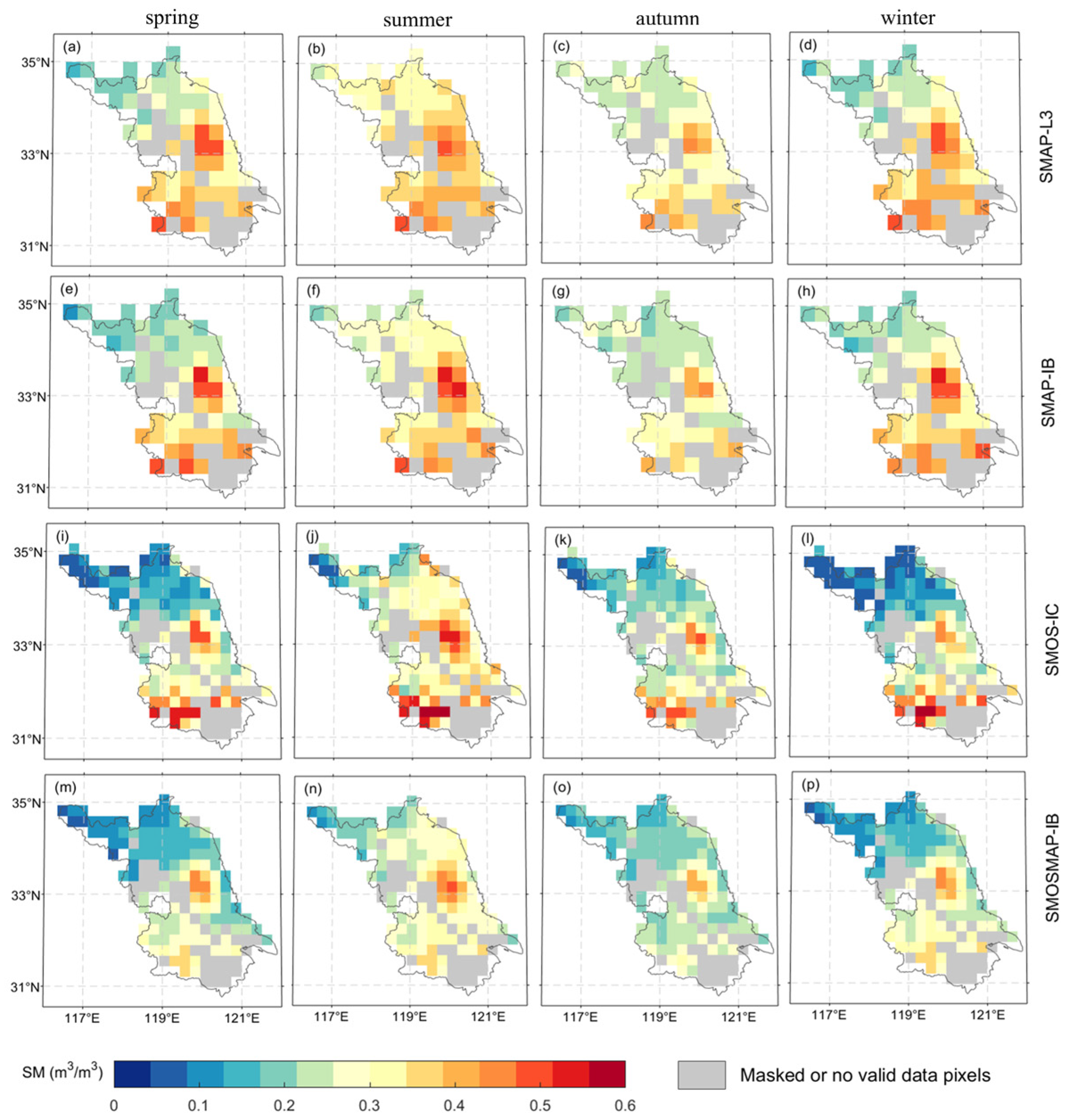
4.1.1. Spatial Patterns

The spatial patterns of SM retrievals from SMAP-L3, SMAP-IB, SMOS-IC, and SMOSMAP-IB exhibit generally consistency across most regions of Jiangsu Province (Figure 2). Specifically, irrespective of the season, nearly all the satellite products demonstrate a drier spatial distribution of SM in the northern regions compared to the central and southern regions. Differently, however, SMOS-IC and SMOSMAP-IB SM products have spatial gradient differences, with SM values ranging from less than 0.1 m³/m³ to greater than 0.5 m³/m³, which are more pronounced than the other three products (Figure 2i–p).

4.1.2. SM Absolute Values

In terms of absolute values of SM estimates, SMAP-L3 and SMAP-IB generally exhibit higher moisture levels than SMOS-IC and SMOSMAP-IB. Considering that both SMOSMAP-IB and SMAP-IB use the same inversion algorithm and soil temperature inputs, the bias between them is mainly due to the warmer fused SMOS-SMAP TB, as SMOS is used as a reference during fusion [18]. This is consistent with the negative correlation between TB and SM [8]; thus, a large TB corresponds to a dry SM. Regarding the different seasons, all four L-band SM products tend to exhibit increased wetness in the northern region of Jiangsu during the summer (Figure 2b,f,j,n).

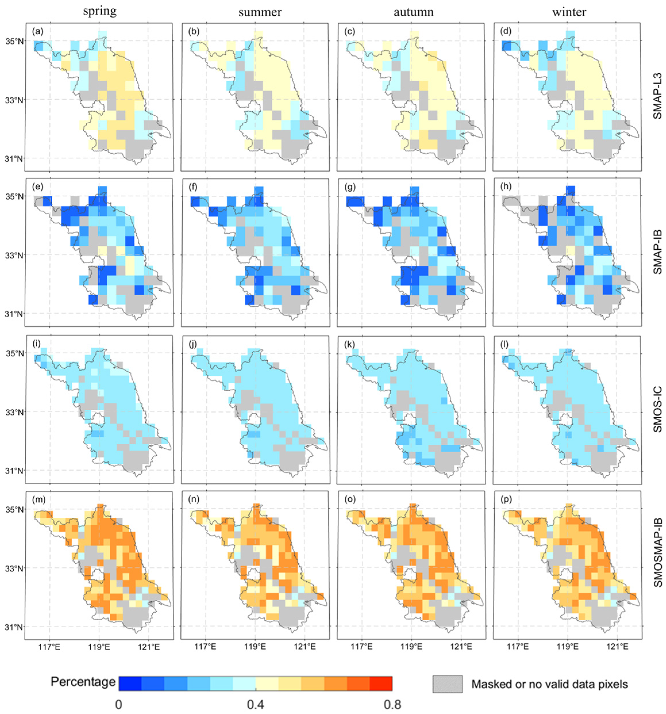
4.1.3. Spatial Coverage and Temporal Availability

The spatial coverage of individual SM products across Jiangsu Province is slightly different (Figure 2). Specifically, SMOS-IC and SMOSMAP-IB have narrower coverage, mainly due to their stricter criteria for excluding pixels affected by urban areas and water bodies. Moreover, owing to the extensive network of water systems, including both rivers and static water bodies in Jiangsu (Figure 1b), it is observed that all four satellite products cannot fully cover the entire region, particularly in the southern part of Jiangsu.

Regarding the availability of temporal observations, there are notable discrepancies in the data provided by the four L-band SM products (Figure 3). Specifically, the temporal availability of SMOS-IC SM retrievals is the lowest among the four products across the four seasons. This feature can be attributed to the fact that SMAP observations are less affected by temporally and spatially varying RFI than SMOS, which is widely reported to suffer from high interference in China [27,32]. It is evident that SMOSMAP-IB, which fuses SMOS and SMAP, offers more observations than any SM product based solely on one of these two sensors (Figure 3m–p). In addition, the percentage of valid observations for the four SM products is highest in the spring and decreases in the winter. This may be due to the presence of ice, snow, and frozen soil during winter, making it difficult to simulate surface dielectric properties [57]. Consequently, none of the current SM products account for retrievals during this period [58].

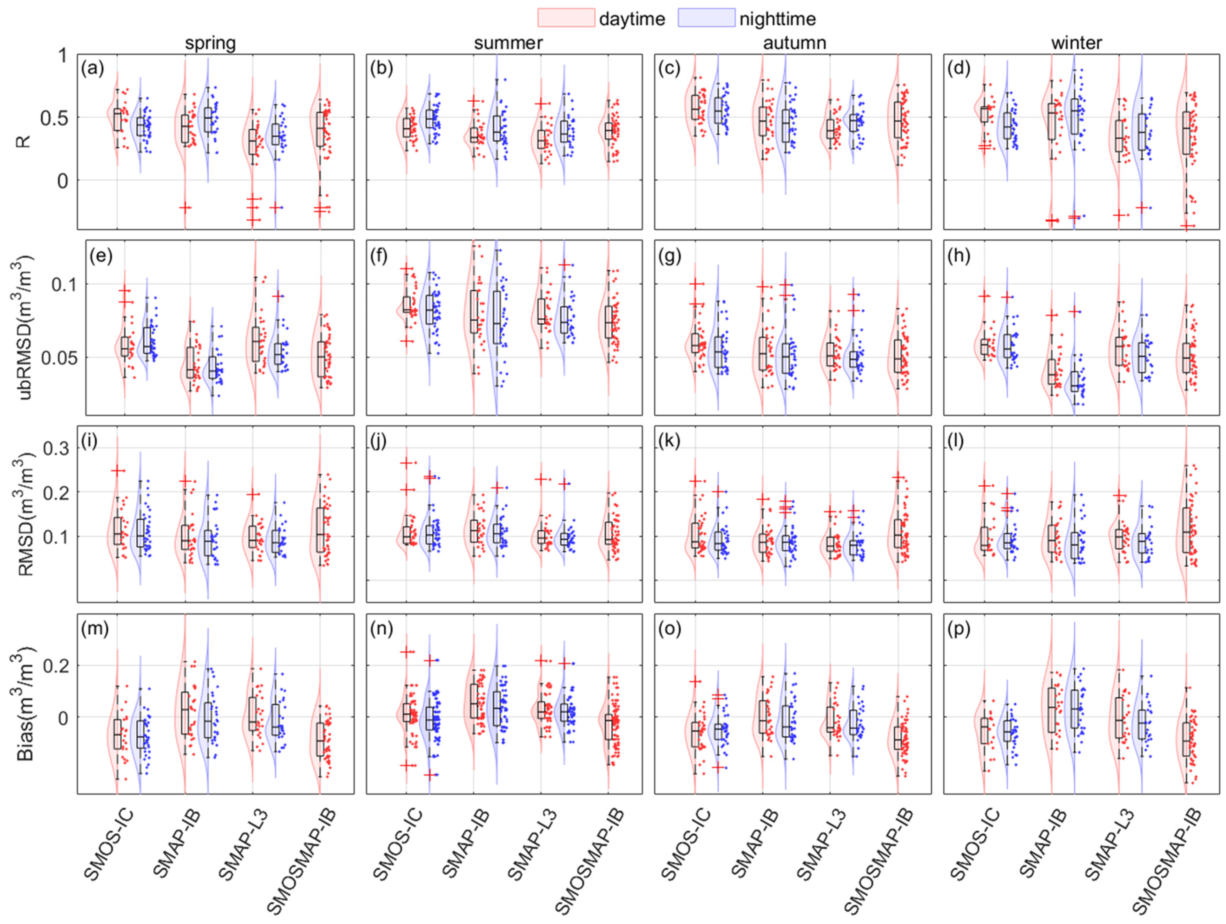
4.2. The Overall and Seasonal Performance of the Four SM Products

To understand the overall performance of the four L-band SM products and their differences across the four seasons, this section utilizes Taylor diagrams and violin plots, which are evaluated against the in situ SM measurements from 2016 to 2022.

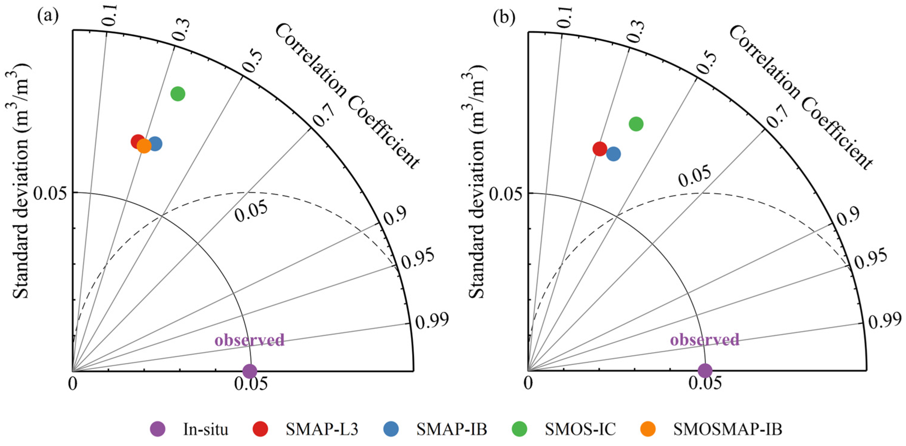
4.2.1. Overall Performance

Figure 4 shows the overall performance of the four SM algorithms in Jiangsu for both morning and afternoon observations, evaluated based on in situ SM measurements from 2016 to 2022. When comparing SM retrievals between a.m. and p.m., both SMAP-IB and SMOS-IC perform better during p.m. observations in terms of R values. This differs from the results of some earlier studies [59,60]. A plausible explanation for this counterintuitive observation is that sustained daytime water stress results in decreased vegetation water content by evening, making the vegetation more transparent [61]. This results in a reduced impact of vegetation on the attenuation of soil emissions, a phenomenon that has been revealed by Zeng et al. [62] and Yi et al. [10]. While SMAP-L3 similarly reflects this pattern, the R values for p.m. observations are only marginally higher than those for a.m. (Figure 4a,b). Among the different products, SMOS-IC and SMAP-IB generally outperform others in capturing the temporal variability of ground observations, particularly during p.m. observations. However, when examining the standard deviation, it is evident that products derived from SMAP satellite observations tend to have lower values compared to those derived solely from SMOS observations (i.e., SMOS-IC).

4.2.2. Seasonal Assessment

Figure 5 summarizes the statistical results of the evaluation metrics for the four satellite SM products during daytime (06:00 a.m.) and nighttime (06:00 p.m.) across the four seasons. While different products exhibit varied performance across individual sites, we represent their overall performance by calculating the median of each metric across all sites, as carried out in studies by [19,20,21]. In terms of the R metrics for the four SM products, SMOS-IC consistently yields better R values (0.405 to 0.564) than the other products during the a.m. observations in all seasons, and from p.m. observations during the summer and autumn. In particular, SMOS-IC exhibits a clear advantage during daytime in the spring, with an R value of 0.524, which far exceeds the second-ranked SMAP-IB (R = 0.424). In contrast, SMAP-L3 shows relatively low R values, especially in the a.m. and p.m. of all seasons except autumn, with median R values below 0.4. SMAP-IB is found to be visibly ahead of SMAP-L3 in the spring and winter, while the difference between them is not significant in the other seasons. Although SMOSMAP-IB enhances spatial and temporal coverage with respect to other L-band SM products, its R value experiences some degradation, particularly in winter, compared to SMAP-IB, which is based solely on SMAP observations. Interestingly, most L-band products achieve improved R values in the autumn compared to other seasons (Figure 5a–d).

Correspondingly, all four L-band SM products also performed respectably in terms of ubRMSD during the autumn. In contrast, all products have degraded ubRMSD performance in the summer, with values greater than 0.060 m³/m³. Among the different products, the lowest ubRMSD value is generally achieved by SMAP-IB, followed by SMOSMAP-IB. In particular, SMAP-IB exhibits potential in winter, with ubRMSD values of 0.038 m³/m³ during the daytime and 0.030 m³/m³ during the nighttime, respectively, satisfying the SMAP mission’s ubRMSD requirement of 0.040 m³/m³ [60]. In addition, both SMAP-IB and SMOSMAP-IB achieved better ubRMSD in the spring compared to the other products (Figure 5e–h). More generally, the latter product, SMOSMAP-IB, remains stable with respect to in situ observations throughout the four seasons. Its ubRMSD is consistently at a low level among the four products, suggesting the great potential for fusing SMOS and SMAP [41]. Consistently, SMOSMAP-IB maintains small RMSD values in all seasons. Apart from this exception, it seems that all products exhibit little variation in RMSD across the seasons, with SMOSMAP-IB generally having larger RMSD with median values of ~0.1 m³/m³. Regarding bias, it is generally observed that both SMOS-IC and SMOSMAP-IB are drier than in situ observations in all seasons except spring (Figure 5m–p), a pattern also noted in the study by Li et al. [18]. Of the four products, both SMAP-IB and SMAP-L3 maintain values close to the in situ observations across all seasons.

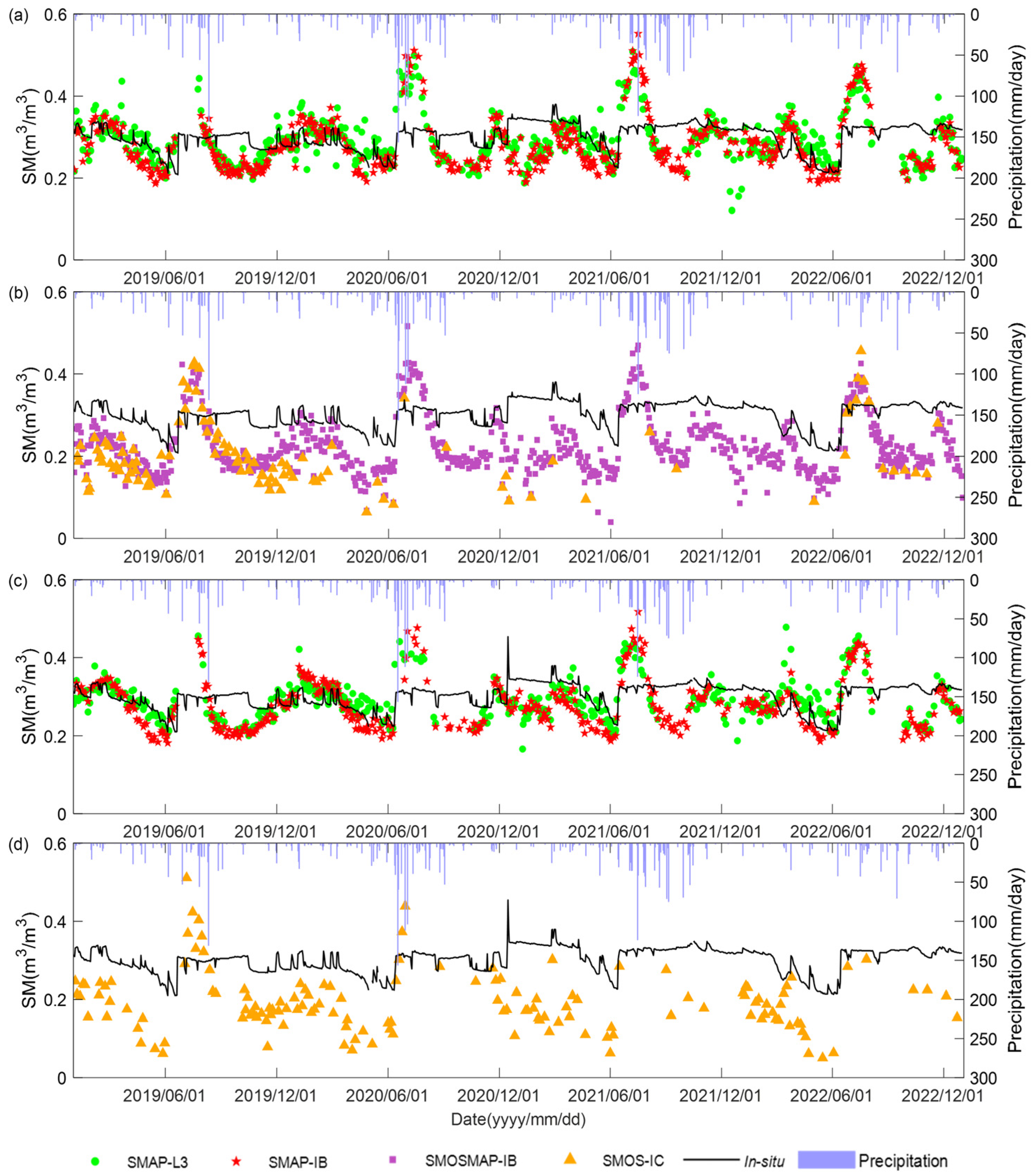
4.3. Time Series Comparison of the Four SM Products

Figure 6 presents the time series of SMAP-L3, SMOS-IC, SMAP-IB, and SMOSMAP-IB SM products from both a.m. and p.m. observations, along with in situ measurements and precipitations bars, at a representative site in FuNing.

Overall, in situ measurements tend to be flatter than the four passive-based SM products both in the morning (top two panels) and afternoon (bottom two panels). It is observed that the SM retrievals from SMAP-L3 and SMAP-IB remain relatively stable between morning and afternoon observations, whereas SMOS-IC shows significant differences. Specifically, SMOS-IC has fewer available observations in the morning, and the afternoon retrievals exhibit a more scattered pattern, likely due to differing sensitivities to RFI between the morning and afternoon observations [63]. Consistent with Section 4.1, SMOSMAP-IB presents more valid data compared to other products. It also shows a similar temporal variation pattern to other SMAP-based SM products, with all aligning well with precipitation, exhibiting increases in SM during rainfall events followed by a subsequent decline.

Seasonally, all four L-band SM values fluctuate significantly in the summer, peaking in July due to higher temperatures and concentrated precipitation. In contrast, the SM values remain relatively stable during autumn and winter, attributed to lower evaporation rates. When compared with in situ measurements, all four SM products are drier than site observations in spring, autumn, and winter, with both SMAP-IB and SMAP-L3 being closest to site observations during most of these periods (Figure 6a,c). In comparison, the absolute SM estimates from both SMOS-IC and SMOSMAP-IB are lower, with values significantly below those of in situ measurements in all seasons except summer. Nevertheless, due to a highly similar retrieval scheme that utilizes the L-MEB model and employs the same soil and vegetation model parameters [8,30], SMOSMAP-IB, like SMAP-IB, provides more consistent information on SM dynamics with a higher number of valid sequences (Figure 6b). Although SMOS-IC displays the least amount of data due to RFI, it still provides a rough indication of the seasonal variability of in situ SM observations, consistent with the results obtained by Fan et al. [27].

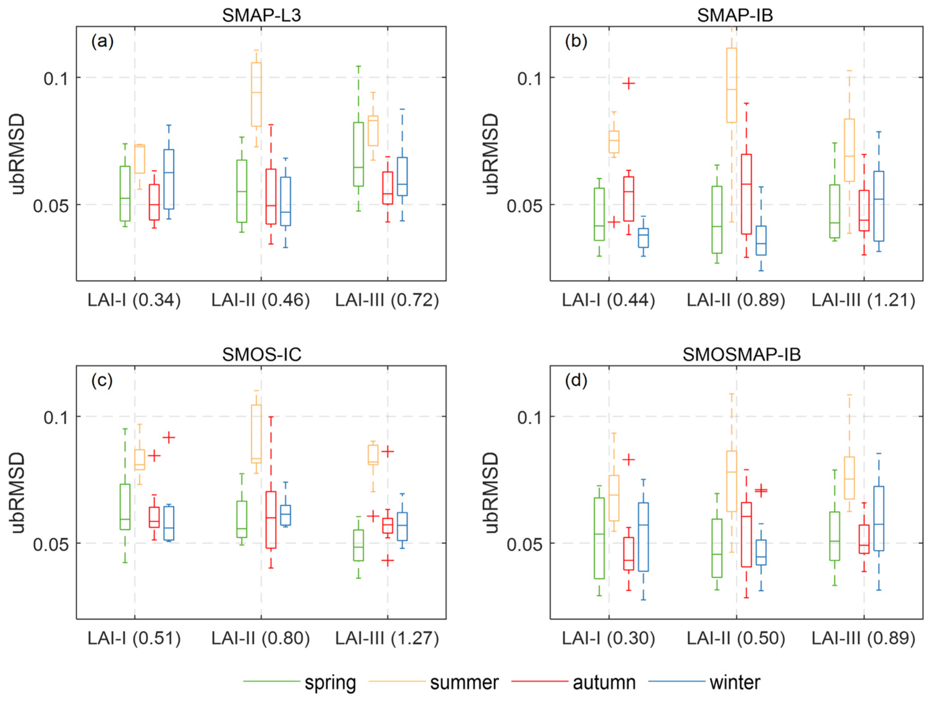
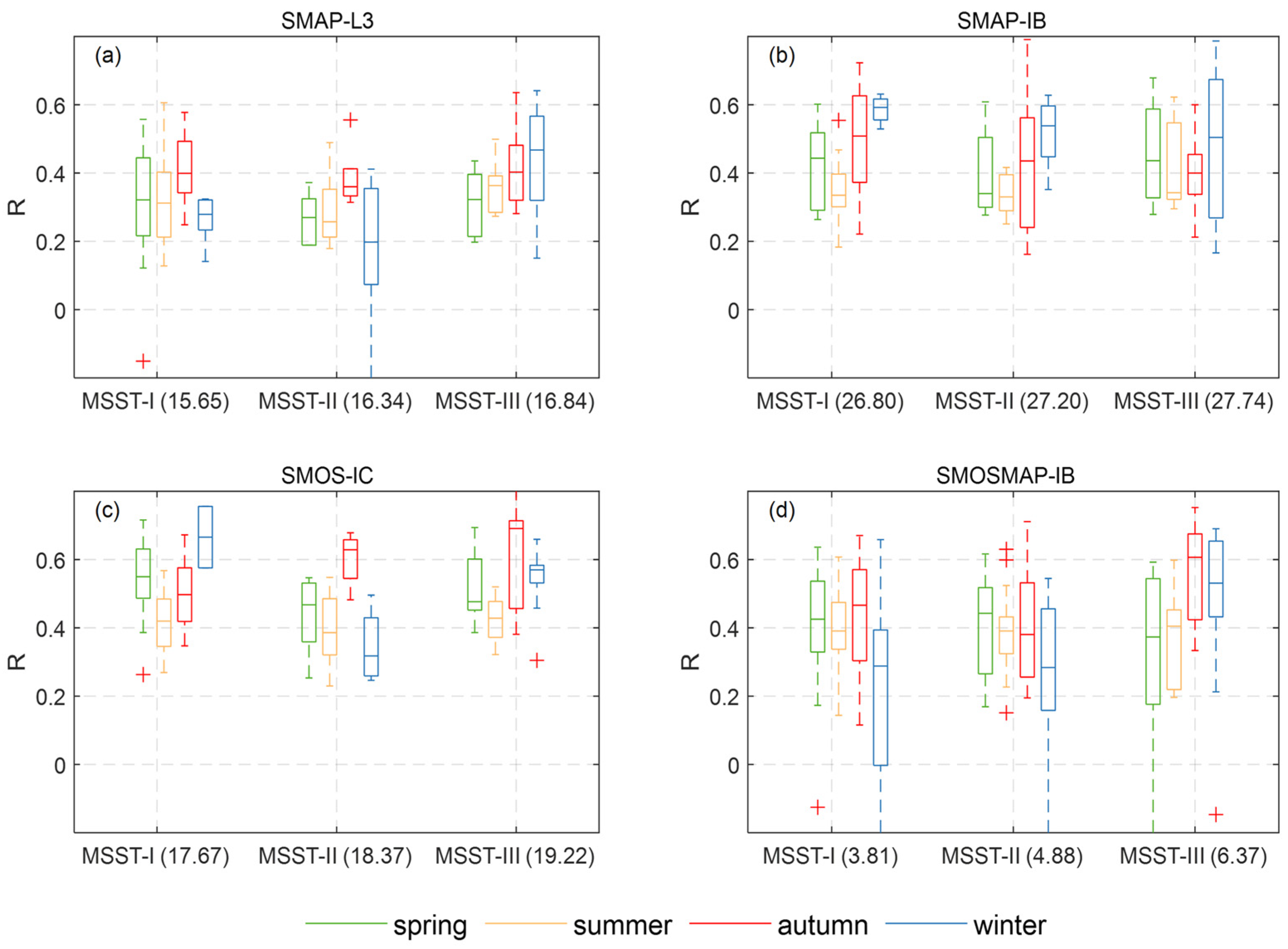
4.4. Impact of Dynamic Factors on the Performance of the Four L-Band SM Retrievals

The above assessment indicates that the performance of the four SM products in Jiangsu Province varies noticeably across different seasons. In this section, we attempt to elucidate the impact of the three pivotal dynamic attributes on these SM products throughout the four seasons, which are LAI, MSST, and MSSM. Note that in this analysis, we consider only the first-order evaluation criteria (R and ubRMSD) for a.m. observation of each product, as the differences between the a.m. and p.m. versions of each product are not sufficient to affect the ranking among products. Additionally, the findings based on p.m. observations (Figures S3–S8) for these three external influencing factors are nearly identical to those from a.m. observations. Therefore, we present only the a.m. results in this section to highlight the key findings.

4.4.1. LAI

To analyze the impact of vegetation on the performance of SM products in more detail, we calculate the distribution of statistical metrics (i.e., R and ubRMSD) as a function of LAI (Figure 7 and Figure 8). Specifically, we create boxplots for these two metrics at the corresponding sites under different LAI categories as carried out by Ma et al. [21]. It is important to note that, since environmental factors also exhibit seasonal dynamics, we define three LAI categories for each season separately to ensure an even distribution of sites. The median LAI values for each category are shown in parentheses. Significant seasonal differences in the effect of LAI on the retrieval performance of different SM products are clearly observed. For instance, a noticeable decrease in the R value is observed as LAI increases in the spring for SMAP-L3 compared to other products. However, in the summer, when LAI reaches its maximum category with a median value of 1.21, SMAP-L3 exhibits the highest R value among the four products (Figure 7b). In the autumn, the R values for all products increase with rising LAI, except for SMOS-IC. While the ranking of products by LAI class varies across seasons, SMOS-IC and SMAP-IB generally perform better in capturing temporal variations in ground SM observations. In particular, SMAP-IB shows leading or comparable R values to the other products during winter (Figure 7d). Additionally, SMOSMAP-IB appears relatively less sensitive to vegetation impacts across seasons, as indicated by minimal fluctuations in its median R values across different LAI levels.

Regarding ubRMSD, contrary to previous studies where an increase in vegetation density typically results in significant degradation of ubRMSD [30,64,65], our findings indicate that this trend is not consistently observed across different products and seasons (Figure 8). For instance, in spring, only SMAP-L3 shows an increase in ubRMSD with rising LAI, while the other products exhibit minimal changes or even a reduction, as observed with SMOS-IC. Moreover, for nearly all products, ubRMSD displays a pattern of initially increasing and then decreasing with LAI variations during summer and autumn. We attribute this partly to the fact that the in situ sites used in this study are predominantly located in agricultural areas of Jiangsu Province (Figure 1), where vegetation density is generally lower. This differs from the more comprehensive validation typically conducted using ISMN, which covers a wider range of vegetation densities.

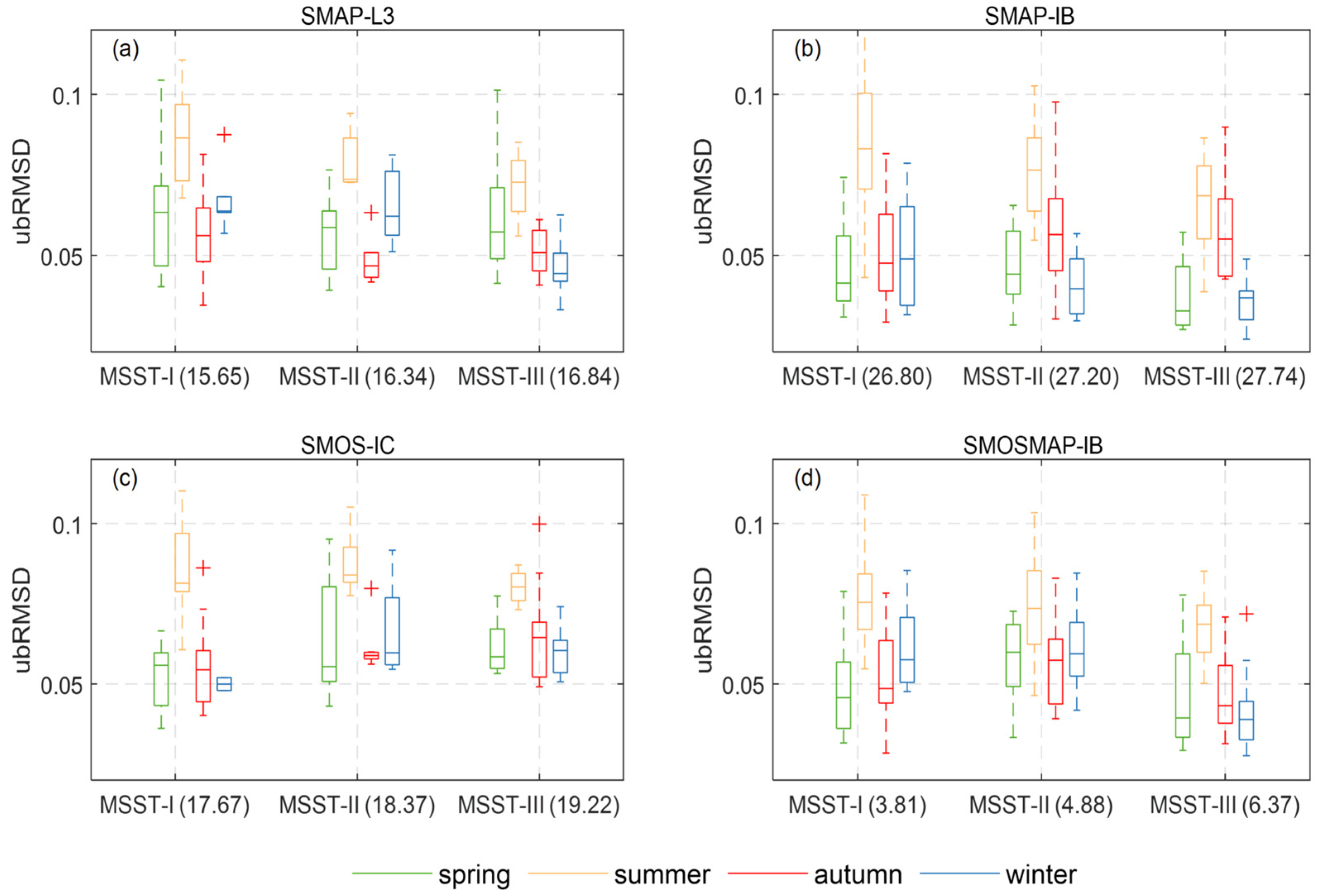
4.4.2. Surface Soil Temperature

With respect to mean surface soil temperature (MSST), the R scores for the four SM retrievals exhibit distinct seasonal variations due to temperature fluctuations characteristic of each season (Figure 9). Specifically, the R values for SMAP-L3 follow a pattern of initially decreasing and then increasing with rising temperatures across all seasons. However, this is not the case for other products. For instance, SMOS-IC shows minimal fluctuations in R values with temperature variations during summer, whereas, in autumn, it demonstrates a marked increase in R values as temperatures rise (Figure 9b,c). Despite both products employing the same L-MEB model retrieval scheme, SMAP-IB consistently shows higher R values than SMOSMAP-IB across most MSST categories during spring, autumn, and winter. Interestingly, this pattern is reversed in summer, when SMOSMAP-IB performs better than SMAP-IB in all MSST categories. It can also be observed that, during winter, when MSST falls into the lowest category, only SMOS-IC and SMAP-IB maintain relatively high R values with a median R value > 0.6, while the other products show a clear degradation in R skill. This disparity may be due to the accuracy of the model temperature inputs used by the different SM inversion algorithms [10,34]. Both SMOSMAP-IB and SMOS-IC rely on the temperature output from the Interim version of the European Centre for Medium-Range Weather Forecasts (ECMWF), whereas SMAP-IB and SMAP-L3 use data from ECMWF’s fifth-generation reanalysis (ERA5) and the Goddard Earth Observing System Model version 5 (GEOS-5). Additionally, an evaluation showed that the temperature output of ERA-Interim could achieve comparable performance within this soil temperature range compared to ERA5 and GEOS-5 [66].

In terms of ubRMSD, a common feature of the four L-band retrievals is that, during summer, all products show a significant improvement in ubRMSD as MSST increases. Moreover, during this season, SMOSMAP-IB has the lowest ubRMSD at all MSST levels. Interestingly, despite ubRMSD remaining at a relatively low level overall, it increases with rising temperatures in autumn for all products except SMAP-L3 (Figure 10). During this season, SMAP-L3 exhibits a noticeably better ubRMSD performance, while SMAP-IB consistently delivers the best performance across most MSST levels in the other seasons, particularly in autumn and winter (Figure 10a,d). It is also evident that different products respond differently to temperature changes across various metrics. For instance, while SMOS-IC shows comparable performance in terms of R values, its ubRMSD remains consistently higher across MSST changes relative to the other products (Figure 9 and Figure 10).

4.4.3. Soil Wetness

Regarding different ground moisture conditions, R values increase with higher moisture levels in spring for all products. However, in other seasons, all four products generally show a decrease in R values as MSSM increases (Figure 11). Among different products, it can be observed that SMOS-IC does not always outperform the others. For example, in winter, when MSSM is at lower levels, SMAP-IB achieves a higher R value, with a median of ~ 0.6, surpassing that of SMOS-IC. Moreover, SMOSMAP-IB generally outperforms SMAP-IB at higher MSSM levels (e.g., at MSSM-III) across different seasons. At these levels, SMAP-L3 demonstrates performance comparable to SMAP-IB, particularly in autumn and winter, despite having lower R values in other seasons. For nearly all products, the R values during summer exhibit minimal fluctuations with changes in MSSM compared to other seasons, with median values not exceeding 0.4.

Interestingly, consistent with the pattern observed for R, as MSSM increases, the ubRMSD values for all products also show improved performance during the spring. For most products during this season, the ubRMSD in the wettest MSSM category falls below 0.05 m³/m³, with SMOSMAP-IB exhibiting the lowest values. Notably, this product also maintains the lowest ubRMSD in the wettest categories during both summer and autumn (Figure 12b,c). However, across most MSSM levels in various seasons, SMAP-IB consistently demonstrates comparable ubRMSD performance. SMAP-L3 is found to exhibit a decrease in ubRMSD as SM increases during spring, autumn, and winter. In contrast, for SMOS-IC, it is difficult to identify a consistent pattern across seasons. This product generally has the highest ubRMSD values under varying SM conditions across different seasons, which is in line with the evaluation study of Ma et al. [64].

5. Discussion

The results above demonstrate the interest in analyzing the accuracy of microwave SM products by season, and all four algorithms have room for improvement. Remarkably, the coverage and the amount of data available for the four SM products are significantly limited after pre-processing. This limitation is primarily due to factors such as the proportion of water bodies, frozen soil conditions, RFI, and errors from algorithmic spurious inversions [8,26,67], which are generally identifiable through the quality markers of each product. In particular, coarse-resolution SM products in Jiangsu Province are especially affected by the extensive water system distribution, highlighting the need for the development of SM products that incorporate water body corrections in the inversion algorithms, or the creation of higher-resolution products to meet the application requirements of various disciplines [4,6,68]. Nonetheless, fusing SMOS and SMAP data can significantly improve the temporal tracking of surface SM changes [18].

Based on the evaluations and comparative results presented in Section 4.2, it is evident that different SM products exhibit significant seasonal performance variations. On one hand, most SM products demonstrate optimal performance in autumn, achieving the highest R values and the lowest ubRMSD values, while both metrics are the poorest in summer. This may be partially attributed to the lower vegetation cover in autumn due to plant senescence. Another possible reason is that the modeled temperatures on which these products are based are more accurate in this season [66,69], as we find that the accuracy of most products responds uniquely to autumn soil temperatures compared to other seasons, with the R metric generally increasing as temperatures rise (Figure 9). However, caution should be taken when interpreting Figure 7, Figure 8, Figure 9, Figure 10, Figure 11 and Figure 12, as they result from numerous interdependent factors affecting SM retrieval accuracy [8,10], many of which are not analyzed in this study (e.g., soil texture, water bodies, etc.). Additionally, this also suggests the potential need to reconsider the evaluation and calibration of certain key radiative transfer variables, such as surface roughness (Hr) and effective scattering albedo (ω), by taking into account their temporal dynamics to develop improved products [40]. Conversely, in the summer, the most likely reason for the poorest performance of all products is the impact of rainfall. Due to the East Asian monsoon, the Jiangsu region typically experiences heavy rainfall during this season (Figure 6). The underlying reason is that rainfall affects the vertical distribution of SM, leading to greater depth discrepancies between satellite measurements (typically within 0–5 cm) and in situ observations (10 cm used here). This is supported by Figure 13, which shows that excluding rainfall periods can significantly improve SM validation accuracy for all four SM products, particularly for the ubRMSD metric, in line with the findings of Colliander et al. [70]. Additionally, water interception by vegetation canopy is another potential influencing factor, particularly for cropland [8].

On the other hand, among the different products, we find that no single SM algorithm consistently holds an absolute advantage under any environmental factors, regardless of the evaluation metric considered (Figure 6, Figure 7 and Figure 8). This is consistent with previous SM evaluation studies [10,30,62,64]. Nevertheless, it can be observed that SMOS-IC has the highest overall R values in most seasons, while SMAP-IB exhibits the lowest ubRMSD values, with SMOSMAP-IB following closely. Although the RFI contamination of SMOS satellite observations in China has been widely reported, SMOS-IC has demonstrated good performance in the Jiangsu region due to algorithm improvements and the application of RFI filtering strategies [27,32,34]. Additionally, we find that the sensitivity of skill metrics for different products to the three analyzed dynamic environmental factors varies across seasons. For instance, the ubRMSD of SMAP-L3 shows a noticeable increase, with rising LAI during the spring, unlike its response to the other two environmental factors. A possible reason for this is that, unlike the other three products, which are entirely independent of optical information, SMAP-L3 incorporates optical data in its VOD retrieval process, potentially integrating information from the latter. As a crucial component of the τ-ω model, errors in VOD retrievals can propagate and accumulate in the SM retrieval results, as evidenced by Gao et al. [28]. Interestingly, compared to other products, SMOS-IC and SMOSMAP-IB are less influenced by external factors in terms of ubRMSD.

There are some limitations in this study. First, due to the limited coverage of in situ data and its mismatch with the spatial resolution of grid-based satellites, traditional point-scale validation methods inevitably introduce representativeness errors [32,34]. Although this study has taken necessary measures, such as using R and ubRMSD as primary evaluation metrics given their lower susceptibility to bias, potential errors may still exist in the absolute values of these metrics. Nevertheless, we also applied the Triple Collocation Analysis (TCA) method, which is based on mathematical statistics, does not require ground truth data, and is unaffected by spatial representativeness errors. By constructing traditional (modeled, active, and passive) triple collocations [26,71], we found that the ranking of R values obtained from TCA is nearly consistent with the site-based validation results presented in this study (Figure S9), demonstrating the robustness of our findings. Furthermore, not only dynamic environmental factors such as vegetation density, soil temperature, and surface soil wetness but also static conditions such as soil properties, land cover, and climatic zones affect the SM inversion, which need to be analyzed comprehensively in combination [59]. While field stations in Jiangsu Province are distributed across various locations (Figure 1), they are still insufficient to cover the full range of environmental conditions, particularly in areas with unique hydrological or vegetation characteristics, which may lead to biased conclusions. However, it is not possible to address all these issues in a single study. Future work will focus on a wider geographical area, aiming to collect more ground-based in situ measurements specifically for agricultural fields through a dense network to improve the generalizability of the validation results of this study. In addition, this needs to be complemented by more detailed studies using the TCA method to reduce the representativeness errors between site-based and satellite observations [21,42]. Another approach is to introduce reliable high-resolution SM products as an intermediary to mitigate the scale effect issue [4,6,68].

6. Conclusions

In this study, based on in situ SM data in Jiangsu province from 2016 to 2022, the performance of four SM products (i.e., SMAP-L3, SMOS-IC, SMAP-IB, and SMOSMAP-IB) under different seasons is evaluated using indicators including R, ubRMSD, RMSD, and bias. Additionally, this study discussed the differences between satellite SM retrievals and in situ observations on external dynamic factors such as LAI, MSST, and MSSM. We find that:

(1) Current products are unable to fully cover the entire Jiangsu province spatially due to their coarse resolution and disturbances such as the influence of static water bodies. Nonetheless, the fusion of SMOS and SMAP can significantly increase the temporal revisit frequency for capturing SM variations compared to products based on a single sensor.

(2) Seasonally, the four products exhibit significant performance differences, with most products showing improved performance in the autumn and the poorest performance in the summer, particularly with respect to the metric ubRMSD. This discrepancy is most likely due to the disturbances caused by summer rainfall, which not only leads to water interception but also affects the vertical distribution of SM and thus increases the differences between in situ measurements and satellite observations.

(3) Among the different products, SMOS-IC generally achieves better R values but has less temporal availability, while SMAP-IB shows the lowest ubRMSD values, followed by SMOSMAP-IB. The sensitivity of different products’ skill metrics to the three dynamic environmental factors varies across seasons. For ubRMSD, SMAP-L3 generally shows an increase with LAI in all four seasons, while SMAP-IB exhibits a notable increase as the soil becomes wetter in the summer. Conversely, wet conditions clearly reduce the R metric values during the autumn for most products.

In summary, our findings indicate that there is room for enhancement in all four SM products, as their overall performance in Jiangsu is not very high compared to the in situ measurements. For instance, few products have a median R value greater than 0.6. Additionally, significant performance differences across different seasons suggest that the use of static model parameters, such as the assumption of time-invariant Hr and ω in current algorithms, needs to be reconsidered. Evaluating the applicability of microwave satellite SM products in Jiangsu not only provides a reference for selecting suitable SM datasets in different periods but also is crucial for improving SM retrieval algorithms. It is expected that our findings will enhance satellite SM algorithms and promote the application of these valuable SM products in terrestrial water, hydrology, energy, and carbon cycles.

References

1. Periasamy, S.; Shanmugam, R.S. Multispectral and Microwave Remote Sensing Models to Survey Soil Moisture and Salinity. Land Degrad. Dev. 2017, 28, 1412–1425. [Google Scholar] [CrossRef]
2. Rodríguez-Fernández, N.; Al Bitar, A.; Colliander, A.; Zhao, T. Soil Moisture Remote Sensing across Scales. Remote Sens. 2019, 11, 190. [Google Scholar] [CrossRef]
3. Klotzsche, A.; Jonard, F.; Looms, M.C.; Kruk, J.V.D.; Huisman, J.A. Measuring Soil Water Content with Ground Penetrating Radar: A Decade of Progress. Vadose Zone J. 2018, 17, 180052. [Google Scholar] [CrossRef]
4. Peng, J.; Albergel, C.; Balenzano, A.; Brocca, L.; Cartus, O.; Cosh, M.H.; Crow, W.T.; Dabrowska-Zielinska, K.; Dadson, S.; Davidson, M.W.J.; et al. A Roadmap for High-Resolution Satellite Soil Moisture Applications—Confronting Product Characteristics with User Requirements. Remote Sens. Environ. 2021, 252, 112162. [Google Scholar] [CrossRef]
5. Lei, F.; Jean-Pierre, W.; Philippe, C.; Chave, J.; Martin, B.; Stephen, S.; Chao, Y.; Ana, B.; Xin, L.; Yuanwei, Q. Siberian Carbon Sink Reduced by Forest Disturbances. Nat. Geosci. 2023, 16, 56–62. [Google Scholar]
6. Wigneron, J.-P.; Ciais, P.; Li, X.; Brandt, M.; Canadell, J.G.; Tian, F.; Wang, H.; Bastos, A.; Fan, L.; Gatica, G.; et al. Global Carbon Balance of the Forest: Satellite-Based L-VOD Results over the Last Decade. Front. Remote Sens. 2024, 5, 1338618. [Google Scholar] [CrossRef]
7. Crow, W.T.; Berg, A.A.; Cosh, M.H.; Loew, A.; Mohanty, B.P.; Panciera, R.; de Rosnay, P.; Ryu, D.; Walker, J.P. Upscaling Sparse Ground-Based Soil Moisture Observations for the Validation of Coarse-Resolution Satellite Soil Moisture Products. Rev. Geophys. 2012, 50, RG2002. [Google Scholar] [CrossRef]
8. Wigneron, J.-P.; Jackson, T.J.; O’Neill, P.; De Lannoy, G.; de Rosnay, P.; Walker, J.P.; Ferrazzoli, P.; Mironov, V.; Bircher, S.; Grant, J.P.; et al. Modelling the Passive Microwave Signature from Land Surfaces: A Review of Recent Results and Application to the L-Band SMOS & SMAP Soil Moisture Retrieval Algorithms. Remote Sens. Environ. 2017, 192, 238–262. [Google Scholar] [CrossRef]
9. Gao, L.; Gao, Q.; Zhang, H.; Li, X.; Chaubell, M.J.; Ebtehaj, A.; Shen, L.; Wigneron, J.-P. A Deep Neural Network Based SMAP Soil Moisture Product. Remote Sens. Environ. 2022, 277, 113059. [Google Scholar] [CrossRef]
10. Yi, C.; Li, X.; Zeng, J.; Fan, L.; Xie, Z.; Gao, L.; Xing, Z.; Ma, H.; Boudah, A.; Zhou, H.; et al. Assessment of Five SMAP Soil Moisture Products Using ISMN Ground-Based Measurements over Varied Environmental Conditions. J. Hydrol. 2023, 619, 129325. [Google Scholar] [CrossRef]
11. Dong, J.; Crow, W.T.; Tobin, K.J.; Cosh, M.H.; Bosch, D.D.; Starks, P.J.; Seyfried, M.; Collins, C.H. Comparison of Microwave Remote Sensing and Land Surface Modeling for Surface Soil Moisture Climatology Estimation. Remote Sens. Environ. 2020, 242, 111756. [Google Scholar] [CrossRef]
12. Ma, H.; Zeng, J.; Zhang, X.; Peng, J.; Li, X.; Fu, P.; Cosh, M.H.; Letu, H.; Wang, S.; Chen, N.; et al. Surface Soil Moisture from Combined Active and Passive Microwave Observations: Integrating ASCAT and SMAP Observations Based on Machine Learning Approaches. Remote Sens. Environ. 2024, 308, 114197. [Google Scholar] [CrossRef]
13. Entekhabi, D.; Njoku, E.G.; O’Neill, P.E.; Kellogg, K.H.; Crow, W.T.; Edelstein, W.N.; Entin, J.K.; Goodman, S.D.; Jackson, T.J.; Johnson, J.; et al. The Soil Moisture Active Passive (SMAP) Mission. Proc. IEEE 2010, 98, 704–716. [Google Scholar] [CrossRef]
14. Kerr, Y.H.; Waldteufel, P.; Wigneron, J.-P.; Delwart, S.; Cabot, F.; Boutin, J.; Escorihuela, M.-J.; Font, J.; Reul, N.; Gruhier, C.; et al. The SMOS Mission: New Tool for Monitoring Key Elements Ofthe Global Water Cycle. Proc. IEEE 2010, 98, 666–687. [Google Scholar] [CrossRef]
15. Dorigo, W.; Wagner, W.; Albergel, C.; Albrecht, F.; Balsamo, G.; Brocca, L.; Chung, D.; Ertl, M.; Forkel, M.; Gruber, A.; et al. ESA CCI Soil Moisture for Improved Earth System Understanding: State-of-the Art and Future Directions. Remote Sens. Environ. 2017, 203, 185–215. [Google Scholar] [CrossRef]
16. Li, X.; Xin, X.; Jiao, J.; Peng, Z.; Zhang, H.; Shao, S.; Liu, Q. Estimating Subpixel Surface Heat Fluxes through Applying Temperature-Sharpening Methods to MODIS Data. Remote Sens. 2017, 9, 836. [Google Scholar] [CrossRef]
17. Liu, Y.Y.; Dorigo, W.A.; Parinussa, R.M.; De Jeu, R.A.M.; Wagner, W.; McCabe, M.F.; Evans, J.P.; Van Dijk, A.I.J.M. Trend-Preserving Blending of Passive and Active Microwave Soil Moisture Retrievals. Remote Sens. Environ. 2012, 123, 280–297. [Google Scholar] [CrossRef]
18. Li, X.; Wigneron, J.-P.; Frappart, F.; Lannoy, G.D.; Fan, L.; Zhao, T.; Gao, L.; Tao, S.; Ma, H.; Peng, Z.; et al. The First Global Soil Moisture and Vegetation Optical Depth Product Retrieved from Fused SMOS and SMAP L-Band Observations. Remote Sens. Environ. 2022, 282, 113272. [Google Scholar] [CrossRef]
19. Zheng, J.; Zhao, T.; Lü, H.; Shi, J.; Cosh, M.H.; Ji, D.; Jiang, L.; Cui, Q.; Lu, H.; Yang, K. Assessment of 24 Soil Moisture Datasets Using a New in Situ Network in the Shandian River Basin of China. Remote Sens. Environ. 2022, 271, 112891. [Google Scholar] [CrossRef]
20. Bai, L.; Lv, X.; Li, X. Evaluation of Two SMAP Soil Moisture Retrievals Using Modeled- and Ground-Based Measurements. Remote Sens. 2019, 11, 2891. [Google Scholar] [CrossRef]
21. Ma, H.; Li, X.; Zeng, J.; Zhang, X.; Dong, J.; Chen, N.; Fan, L.; Sadeghi, M.; Frappart, F.; Liu, X.; et al. An Assessment of L-Band Surface Soil Moisture Products from SMOS and SMAP in the Tropical Areas. Remote Sens. Environ. 2023, 284, 113344. [Google Scholar] [CrossRef]
22. Xing, Z.; Li, X.; Fan, L.; Frappart, F.; Kim, H.; Lanka, K.; Konkathi, P.; Liu, Y.; Zhao, L.; Wigneron, J.-P.; et al. Seasonal-Scale Intercomparison of SMAP and Fused SMOS-SMAP Soil Moisture Products. Front. Remote Sens. 2024, 5, 1440891. [Google Scholar] [CrossRef]
23. Colliander, A.; Kerr, Y.; Wigneron, J.-P.; Al-Yaari, A.; Rodriguez-Fernandez, N.; Li, X.; Chaubell, J.; Richaume, P.; Mialon, A.; Asanuma, J.; et al. Performance of SMOS Soil Moisture Products Over Core Validation Sites. IEEE Geosci. Remote Sens. Lett. 2023, 20, 1–5. [Google Scholar] [CrossRef]
24. Duzenli, E.; Yucel, I.; Yilmaz, M.T. Evaluation of the Fully Coupled WRF and WRF-Hydro Modelling System Initiated with Satellite-Based Soil Moisture Data. Hydrol. Sci. J. 2024, 69, 691–708. [Google Scholar] [CrossRef]
25. Wang, Z.; Che, T.; Zhao, T.; Dai, L.; Li, X.; Wigneron, J.P. Evaluation of SMAP, SMOS, and AMSR2 Soil Moisture Products Based on Distributed Ground Observation Network in Cold and Arid Regions of China. IEEE J. Sel. Top. Appl. Earth Obs. Remote Sens. 2021, 14, 8955–8970. [Google Scholar] [CrossRef]
26. Kim, H.; Crow, W.; Li, X.; Wagner, W.; Hahn, S.; Lakshmi, V. True Global Error Maps for SMAP, SMOS, and ASCAT Soil Moisture Data Based on Machine Learning and Triple Collocation Analysis. Remote Sens. Environ. 2023, 298, 113776. [Google Scholar] [CrossRef]
27. Fan, L.; Xing, Z.; Lannoy, G.D.; Frappart, F.; Peng, J.; Zeng, J.; Li, X.; Yang, K.; Zhao, T.; Shi, J.; et al. Evaluation of Satellite and Reanalysis Estimates of Surface and Root-Zone Soil Moisture in Croplands of Jiangsu Province, China. Remote Sens. Environ. 2022, 282, 113283. [Google Scholar] [CrossRef]
28. Gao, L.; Ebtehaj, A.; Chaubell, M.J.; Sadeghi, M.; Li, X.; Wigneron, J.-P. Reappraisal of SMAP Inversion Algorithms for Soil Moisture and Vegetation Optical Depth. Remote Sens. Environ. 2021, 264, 112627. [Google Scholar] [CrossRef]
29. Bai, Y.; Zhao, T.; Jia, L.; Cosh, M.H.; Shi, J.; Peng, Z.; Li, X.; Wigneron, J.-P. A Multi-Temporal and Multi-Angular Approach for Systematically Retrieving Soil Moisture and Vegetation Optical Depth from SMOS Data. Remote Sens. Environ. Interdiscip. J. 2022, 280, 113190. [Google Scholar] [CrossRef]
30. Li, X.; Wigneron, J.-P.; Fan, L.; Frappart, F.; Yueh, S.H.; Colliander, A.; Ebtehaj, A.; Gao, L.; Fernandez-Moran, R.; Liu, X.; et al. A New SMAP Soil Moisture and Vegetation Optical Depth Product (SMAP-IB): Algorithm, Assessment and Inter-Comparison. Remote Sens. Environ. 2022, 271, 112921. [Google Scholar] [CrossRef]
31. Al-Yaari, A.; Wigneron, J.-P.; Ducharne, A.; Kerr, Y.; de Rosnay, P.; de Jeu, R.; Govind, A.; Al Bitar, A.; Albergel, C.; Muñoz-Sabater, J.; et al. Global-Scale Evaluation of Two Satellite-Based Passive Microwave Soil Moisture Datasets (SMOS and AMSR-E) with Respect to Land Data Assimilation System Estimates. Remote Sens. Environ. 2014, 149, 181–195. [Google Scholar] [CrossRef]
32. Wigneron, J.-P.; Li, X.; Frappart, F.; Fan, L.; Al-Yaari, A.; De Lannoy, G.; Liu, X.; Wang, M.; Le Masson, E.; Moisy, C. SMOS-IC Data Record of Soil Moisture and L-VOD: Historical Development, Applications and Perspectives. Remote Sens. Environ. 2021, 254, 112238. [Google Scholar] [CrossRef]
33. Li, X.; Al-Yaari, A.; Schwank, M.; Fan, L.; Frappart, F.; Swenson, J.; Wigneron, J.-P. Compared Performances of SMOS-IC Soil Moisture and Vegetation Optical Depth Retrievals Based on Tau-Omega and Two-Stream Microwave Emission Models. Remote Sens. Environ. 2020, 236, 111502. [Google Scholar] [CrossRef]
34. Xing, Z.; Fan, L.; Zhao, L.; De Lannoy, G.; Frappart, F.; Peng, J.; Li, X.; Zeng, J.; Al-Yaari, A.; Yang, K.; et al. A First Assessment of Satellite and Reanalysis Estimates of Surface and Root-Zone Soil Moisture over the Permafrost Region of Qinghai-Tibet Plateau. Remote Sens. Environ. 2021, 265, 112666. [Google Scholar] [CrossRef]
35. Fernandez-Moran, R.; Al-Yaari, A.; Mialon, A.; Mahmoodi, A.; Al Bitar, A.; De Lannoy, G.; Rodriguez-Fernandez, N.; Lopez-Baeza, E.; Kerr, Y.; Wigneron, J.P. SMOS-IC: An Alternative SMOS Soil Moisture and Vegetation Optical Depth Product. Remote Sens. 2017, 9, 457. [Google Scholar] [CrossRef]
36. Chaubell, M.J.; Yueh, S.H.; Dunbar, R.S.; Colliander, A.; Chen, F.; Chan, S.K.; Entekhabi, D.; Bindlish, R.; O’Neill, P.E.; Asanuma, J.; et al. Improved SMAP Dual-Channel Algorithm for the Retrieval of Soil Moisture. IEEE Trans. Geosci. Remote Sens. 2020, 58, 3894–3905. [Google Scholar] [CrossRef]
37. O’neill, P.; Bindlish, R.; Chan, S.; Njoku, E.; Jackson, T. Algorithm Theoretical Basis Document. In Level 2 & 3 Soil Moisture (Passive) Data Products; Hydrology and Earth System Sciences (HESS): Göttingen, Germany, 2018. [Google Scholar]
38. O’Neill, P.E.; Chan, S.; Njoku, E.G.; Jackson, T.; Bindlish, R.; Chaubell, J. SMAP L3 Radiometer Global Daily 36 km EASE-Grid Soil Moisture, Version 8; NASA National Snow and Ice Data Center Distributed Active Archive Center: Boulder, CO, USA, 2021. [Google Scholar]
39. Li, X.; Fernandez-Moran, R.; Frappart, F.; Fan, L.; De Lannoy, G.; Liu, X.; Wang, H.; Xing, Z.; Wang, M.; Xiao, Y.; et al. Alternate INRAE-Bordeaux Soil Moisture and L-Band Vegetation Optical Depth Products from SMOS and SMAP: Current Status and Overview. In Proceedings of the IGARSS 2023—2023 IEEE International Geoscience and Remote Sensing Symposium, Pasadena, CA, USA, 16–21 July 2023; pp. 2629–2632. [Google Scholar]
40. Li, X.; Wigncron, J.-P.; Frappart, F.; Fan, L.; De Lannoy, G.; Konings, A.G.; Liu, X.; Wang, M.; Fernandez-Moran, R.; Al-Yaari, A.; et al. Global Long-Term Brightness Temperature Record from L-Band SMOS and Smap Observations. In Proceedings of the 2021 IEEE International Geoscience and Remote Sensing Symposium IGARSS, Brussels, Belgium, 11–16 July 2021; pp. 6108–6111. [Google Scholar]
41. Bindlish, R.; Chan, S.; Colliander, A.; Kerr, Y.; Jackson, T.J. Integrated SMAP and SMOS Soil Moisture Observations. In Proceedings of the IGARSS 2019—2019 IEEE International Geoscience and Remote Sensing Symposium, Yokohama, Japan, 28 July–2 August 2019; pp. 5370–5373. [Google Scholar]
42. Gruber, A.; Lannoy, G.D.; Albergel, C.; Al-Yaari, A.; Brocca, L.; Calvet, J.-C.; Colliander, A.; Cosh, M.; Crow, W.; Dorigo, W.; et al. Validation Practices for Satellite Soil Moisture Retrievals: What Are (the) Errors? Remote Sens. Environ. 2020, 244, 111806. [Google Scholar] [CrossRef]
43. Dorigo, W.A.; Xaver, A.; Vreugdenhil, M.; Gruber, A.; Hegyiová, A.; Sanchis-Dufau, A.D.; Zamojski, D.; Cordes, C.; Wagner, W.; Drusch, M. Global Automated Quality Control of In Situ Soil Moisture Data from the International Soil Moisture Network. Vadose Zone J. 2013, 12, vzj2012.0097. [Google Scholar] [CrossRef]
44. Cui, C.; Xu, J.; Zeng, J.; Chen, K.S.; Bai, X.; Lu, H.; Chen, Q.; Zhao, T. Soil Moisture Mapping from Satellites: An Intercomparison of SMAP, SMOS, FY3B, AMSR2, and ESA CCI over Two Dense Network Regions at Different Spatial Scales. Remote Sens. 2018, 10, 33. [Google Scholar] [CrossRef]
45. Zeng, J.; Chen, K.S.; Cui, C.; Bai, X. A Physically Based Soil Moisture Index from Passive Microwave Brightness Temperatures for Soil Moisture Variation Monitoring. IEEE Trans. Geosci. Remote Sens. 2019, 58, 2782–2795. [Google Scholar] [CrossRef]
46. Hersbach, H.; de Rosnay, P.; Bell, B.; Schepers, D.; Simmons, A.; Soci, C.; Abdalla, S.; Alonso-Balmaseda, M.; Balsamo, G.; Bechtold, P.; et al. Operational Global Reanalysis: Progress, Future Directions and Synergies with NWP; ECMWF: Reading, UK, 2018. [Google Scholar]
47. Friedl, M.A.; Sulla-Menashe, D.; Tan, B.; Schneider, A.; Ramankutty, N.; Sibley, A.; Huang, X. MODIS Collection 5 Global Land Cover: Algorithm Refinements and Characterization of New Datasets. Remote Sens. Environ. 2010, 114, 168–182. [Google Scholar] [CrossRef]
48. Entekhabi, D.; Reichle, R.H.; Koster, R.D.; Crow, W.T. Performance Metrics for Soil Moisture Retrievals and Application Requirements Dara Entekhabi. J. Hydrometeorol. 2010, 11, 832–840. [Google Scholar] [CrossRef]
49. Wang, M.; Wigneron, J.-P.; Sun, R.; Fan, L.; Frappart, F.; Tao, S.; Chai, L.; Li, X.; Liu, X.; Ma, H.; et al. A Consistent Record of Vegetation Optical Depth Retrieved from the AMSR-E and AMSR2 X-Band Observations. Int. J. Appl. Earth Obs. Geoinf. 2021, 105, 102609. [Google Scholar] [CrossRef]
50. Moriasi, D.; Arnold, J.G.; van Liew, M.W.; Bingner, R.L.; Harmel, R.D.; Veith, T.L. Model Evaluation Guidelines for Systematic Quantification of Accuracy in Watershed Simulations. Trans. ASABE 2007, 50, 885–900. [Google Scholar] [CrossRef]
51. Gruber, A.; Su, C.-H.; Zwieback, S.; Crow, W.; Dorigo, W.; Wagner, W. Recent Advances in (Soil Moisture) Triple Collocation Analysis. Int. J. Appl. Earth Obs. Geoinf. 2016, 45, 200–211. [Google Scholar] [CrossRef]
52. Tavakol, A.; Rahmani, V.; Quiring, S.M.; Kumar, S.V. Evaluation Analysis of NASA SMAP L3 and L4 and SPoRT-LIS Soil Moisture Data in the United States. Remote Sens. Environ. 2019, 229, 234–246. [Google Scholar] [CrossRef]
53. Yang, S.; Li, R.; Wu, T.; Hu, G.; Xiao, Y.; Du, Y.; Zhu, X.; Ni, J.; Ma, J.; Zhang, Y.; et al. Evaluation of Reanalysis Soil Temperature and Soil Moisture Products in Permafrost Regions on the Qinghai-Tibetan Plateau. Geoderma 2020, 377, 114583. [Google Scholar] [CrossRef]
54. Kolassa, J.; Reichle, R.H.; Liu, Q.; Alemohammad, S.H.; Gentine, P.; Aida, K.; Asanuma, J.; Bircher, S.; Caldwell, T.; Colliander, A.; et al. Estimating Surface Soil Moisture from SMAP Observations Using a Neural Network Technique. Remote Sens. Environ. 2018, 204, 43–59. [Google Scholar] [CrossRef]
55. Zeng, J.; Shi, P.; Chen, K.-S.; Ma, H.; Bi, H.; Cui, C. Assessment and Error Analysis of Satellite Soil Moisture Products Over the Third Pole. IEEE Trans. Geosci. Remote Sens. 2022, 60, 1–18. [Google Scholar] [CrossRef]
56. Al-Yaari, A.; Wigneron, J.-P.; Kerr, Y.; Rodriguez-Fernandez, N.; O’Neill, P.E.; Jackson, T.J.; De Lannoy, G.J.M.; Al Bitar, A.; Mialon, A.; Richaume, P.; et al. Evaluating Soil Moisture Retrievals from ESA’s SMOS and NASA’s SMAP Brightness Temperature Datasets. Remote Sens. Environ. 2017, 193, 257–273. [Google Scholar] [CrossRef]
57. Owe, M.; De Jeu, R.; Holmes, T. Multisensor Historical Climatology of Satellite-Derived Global Land Surface Moisture. J. Geophys. Res. Earth Surf. 2008, 113, F01002. [Google Scholar] [CrossRef]
58. Kumawat, D.; Ebtehaj, A.; Schwank, M.; Li, X.; Wigneron, J.-P. Global Estimates of L-Band Vegetation Optical Depth and Soil Permittivity of Snow-Covered Boreal Forests and Permafrost Landscape Using SMAP Satellite Data. Remote Sens. Environ. 2024, 306, 114145. [Google Scholar] [CrossRef]
59. Zhang, S.S.; Kim, S.; Sharma, A. A Comprehensive Validation of the SMAP Enhanced Level-3 Soil Moisture Product Using Ground Measurements over Varied Climates and Landscapes. Remote Sens. Environ. Interdiscip. J. 2019, 223, 82–94. [Google Scholar] [CrossRef]
60. Chan, S.K.; Bindlish, R.; O’Neill, P.; Jackson, T.; Kerr, Y.; Njoku, E.; Dunbar, S.; Chaubell, J.; Piepmeier, J.; Yueh, S.; et al. Development and Assessment of the SMAP Enhanced Passive Soil Moisture Product. Remote Sens. Environ. 2018, 204, 931–941. [Google Scholar] [CrossRef]
61. Wang, F.; Harindintwali, J.D.; Wei, K.; Shan, Y.; Mi, Z.; Costello, M.J.; Grunwald, S.; Feng, Z.; Wang, F.; Guo, Y.; et al. Climate Change: Strategies for Mitigation and Adaptation. Innov. Geosci. 2023, 1, 100015–100095. [Google Scholar] [CrossRef]
62. Zeng, J.; Li, Z.; Chen, Q.; Bi, H.; Qiu, J.; Zou, P. Evaluation of Remotely Sensed and Reanalysis Soil Moisture Products over the Tibetan Plateau Using In-Situ Observations. Remote Sens. Environ. 2015, 163, 91–110. [Google Scholar] [CrossRef]
63. Yang, H.; Ciais, P.; Frappart, F.; Li, X.; Brandt, M.; Fensholt, R.; Fan, L.; Saatchi, S.; Besnard, S.; Deng, Z.; et al. Global Increase in Biomass Carbon Stock Dominated by Growth of Northern Young Forests over Past Decade. Nat. Geosci. 2023, 16, 886–892. [Google Scholar] [CrossRef]
64. Ma, H.; Zeng, J.; Chen, N.; Zhang, X.; Cosh, M.H.; Wang, W. Satellite Surface Soil Moisture from SMAP, SMOS, AMSR2 and ESA CCI: A Comprehensive Assessment Using Global Ground-Based Observations. Remote Sens. Environ. 2019, 231, 111215. [Google Scholar] [CrossRef]
65. Al-Yaari, A.; Wigneron, J.P.; Dorigo, W.; Colliander, A.; Pellarin, T.; Hahn, S.; Mialon, A.; Richaume, P.; Fernandez-Moran, R.; Fan, L.; et al. Assessment and Inter-Comparison of Recently Developed/Reprocessed Microwave Satellite Soil Moisture Products Using ISMN Ground-Based Measurements. Remote Sens. Environ. 2019, 224, 289–303. [Google Scholar] [CrossRef]
66. Ma, H.; Zeng, J.; Zhang, X.; Fu, P.; Zheng, D.; Wigneron, J.P.; Chen, N.; Niyogi, D. Evaluation of Six Satellite- and Model-Based Surface Soil Temperature Datasets Using Global Ground-Based Observations. Remote Sens. Environ. 2021, 264, 112605. [Google Scholar] [CrossRef]
67. Calvet, J.C.; Wigneron, J.P.; Walker, J.; Karbou, F.; Chanzy, A.; Albergel, C. Sensitivity of Passive Microwave Observations to Soil Moisture and Vegetation Water Content: L-Band to W-Band. IEEE Trans. Geosci. Remote Sens. 2011, 49, 1190–1199. [Google Scholar] [CrossRef]
68. Bauer-Marschallinger, B.; Freeman, V.; Cao, S.; Paulik, C.; Schaufler, S.; Stachl, T.; Modanesi, S.; Massari, C.; Ciabatta, L.; Brocca, L.; et al. Toward Global Soil Moisture Monitoring with Sentinel-1: Harnessing Assets and Overcoming Obstacles. IEEE Trans. Geosci. Remote Sens. 2019, 57, 520–539. [Google Scholar] [CrossRef]
69. Xiao, Y.; Li, X.; Fan, L.; Lannoy, G.D.; Peng, J.; Frappart, F.; Ebtehaj, A.; Rosnay, P.D.; Xing, Z.; Yu, L.; et al. Optimal Model-Based Temperature Inputs for Global Soil Moisture and Vegetation Optical Depth Retrievals from SMAP. Remote Sens. Environ. 2024, 311, 114240. [Google Scholar] [CrossRef]
70. Colliander, A.; Jackson, T.J.; Berg, A.; Bosch, D.D.; Caldwell, T.; Chan, S.; Cosh, M.H.; Collins, C.H.; Martínez-Fernández, J.; McNairn, H.; et al. Effect of Rainfall Events on SMAP Radiometer-Based Soil Moisture Accuracy Using Core Validation Sites. J. Hydrometeorol. 2020, 21, 255–264. [Google Scholar] [CrossRef]
71. Kim, H.; Wigneron, J.-P.; Kumar, S.; Dong, J.; Wagner, W.; Cosh, M.H.; Bosch, D.D.; Collins, C.H.; Starks, P.J.; Seyfried, M.; et al. Global Scale Error Assessments of Soil Moisture Estimates from Microwave-Based Active and Passive Satellites and Land Surface Models over Forest and Mixed Irrigated/Dryland Agriculture Regions. Remote Sens. Environ. 2020, 251, 112052. [Google Scholar] [CrossRef]
Figure 1. Overview of the study area: (a) Land cover type (International Geosphere–Biosphere Programme (IGBP) land cover classification scheme). (b) Distribution of ground measurement stations (purple triangles).
Remotesensing 16 04235 g001
Figure 2. Averaged daytime SM (m3/m3) values from 2016 to 2022 for the four L-band SM products. Grey values indicate “Masked or no valid data pixels”. (ad) SMAP-L3; (eh) SMAP-IB; (il) SMOS-IC; (mp) SMOSMAP-IB.
Remotesensing 16 04235 g002
Figure 3. Percentage of data availability for four SM products from daytime observations between 2016 and 2022. Grey values indicate “Masked or no valid data pixels”. Note that the percentage calculation is based on the ratio of actual available days to the total days in each season. (ad) SMAP-L3; (eh) SMAP-IB; (il) SMOS-IC; (mp) SMOSMAP-IB.
Remotesensing 16 04235 g003
Figure 4. Taylor diagrams of the median error metrics for the four SM products evaluated against in situ observations during a.m. (a) and p.m. (b) observation from 2016 to 2022.
Remotesensing 16 04235 g004
Figure 5. Seasonal performance metrics for the four SM products including R, ubRMSD, RMSD, and bias for both daytime (a.m.) and nighttime (p.m.) observations. (ad) R; (eh) ubRMSD; (il) RMSD; (mp) Bias.
Remotesensing 16 04235 g005
Figure 6. Time series of the four SM products and in situ measurements over FuNing station for both a.m. (a,b) and p.m. (c,d) observations between 2019 and 2022. Daily precipitation (mm/day) is shown as a bar chart.
Remotesensing 16 04235 g006
Figure 7. Boxplot of R metric statistical comparisons between the four L–band SM products and in situ measurements by different LAI levels during the four seasons. The values in parentheses are the medians of LAI. (a) SMAP-L3; (b) SMAP-IB; (c) SMOS-IC; (d) SMOSMAP-IB.
Remotesensing 16 04235 g007
Figure 8. Boxplot of ubRMSD metric statistical comparisons between the four L-band SM products and in situ measurements by different LAI levels during the four seasons. The values in parentheses are the medians of LAI. (a) SMAP-L3; (b) SMAP-IB; (c) SMOS-IC; (d) SMOSMAP-IB.
Remotesensing 16 04235 g008
Figure 9. Boxplot of R metric statistical comparisons between the four L-band SM products and in situ measurements by different MSST levels during the four seasons. The values in parentheses are the medians of MSST. (a) SMAP-L3; (b) SMAP-IB; (c) SMOS-IC; (d) SMOSMAP-IB.
Remotesensing 16 04235 g009
Figure 10. Boxplot of ubRMSD metric statistical comparisons between the four L-band SM products and in situ measurements by different MSST levels during the four seasons. The values in parentheses are the medians of MSST. (a) SMAP-L3; (b) SMAP-IB; (c) SMOS-IC; (d) SMOSMAP-IB.
Remotesensing 16 04235 g010
Figure 11. Boxplot of R metric statistical comparisons between the four L-band SM products and in situ measurements by different MSSM levels during the four seasons. The values in parentheses are the medians of MSSM. (a) SMAP-L3; (b) SMAP-IB; (c) SMOS-IC; (d) SMOSMAP-IB.
Remotesensing 16 04235 g011
Figure 12. Boxplot of ubRMSD metric statistical comparisons between the four L-band SM products and in situ measurements by different MSSM levels during the four seasons. The values in parentheses are the medians of MSSM. (a) SMAP-L3; (b) SMAP-IB; (c) SMOS-IC; (d) SMOSMAP-IB.
Remotesensing 16 04235 g012
Figure 13. Density plots of four SM products compared with in situ data at Hai’an station. The background color represents rainfall, with darker shades indicating higher rainfall amounts. The blue and red numbers in each plot indicate the first-order validation metrics before and after excluding observations on rainy days. (a) SMAP-L3; (b) SMAP-IB; (c) SMOS-IC; (d) SMOSMAP-IB.
Remotesensing 16 04235 g013