Unsupervised PolSAR Image Classification Based on Superpixel Pseudo-Labels and a Similarity-Matching Network

Abstract

Supervised polarimetric synthetic aperture radar (PolSAR) image classification demands a large amount of precisely labeled data. However, such data are difficult to obtain. Therefore, many unsupervised methods have been proposed for unsupervised PolSAR image classification. The classification maps of unsupervised methods contain many high-confidence samples. These samples, which are often ignored, can be used as supervisory information to improve classification performance on PolSAR images. This study proposes a new unsupervised PolSAR image classification framework. The framework combines high-confidence superpixel pseudo-labeled samples and semi-supervised classification methods. The experiments indicated that this framework could achieve higher-level effectiveness in unsupervised PolSAR image classification. First, superpixel segmentation was performed on PolSAR images, and the geometric centers of the superpixels were generated. Second, the classification maps of rotation-domain deep mutual information (RDDMI), an unsupervised PolSAR image classification method, were used as the pseudo-labels of the central points of the superpixels. Finally, the unlabeled samples and the high-confidence pseudo-labeled samples were used to train an excellent semi-supervised method, similarity matching (SimMatch). Experiments on three real PolSAR datasets illustrated that, compared with the excellent RDDMI, the accuracy of the proposed method was increased by 1.70%, 0.99%, and 0.8%. The proposed framework provides significant performance improvements and is an efficient method for improving unsupervised PolSAR image classification.

1. Introduction

Polarimetric synthetic aperture radar (PolSAR) has drawn significant attention because it can operate all day and night. A polarization scattering matrix can provide rich feature information that is widely used in land cover classification. In the field of PolSAR image classification, various unsupervised, semi-supervised, and supervised methods have been proposed. A large number of accurately labeled data are necessary in supervised classification methods. Unsupervised learning only uses the similarity relationships between samples to train models without labeled data. PolSAR images often do not have sufficient accurately labeled samples. The accurately labeled samples require significant manpower and time. Therefore, people are increasingly concerned about unsupervised methods.

Recently, many unsupervised methods have been proposed.The maximum likelihood classification [1] has been widely used and developed. This method proposed a new distance metric derived based on the complex Wishart distribution [2]. Pottier et al. [3] proposed a method using $H/\alpha$ to initialize the iterative Wishart classifier. Cao et al. [4] referred to this idea and used $H/\alpha /A-Span$ to initialize the Wishart classifier. Lee et al. [5] also proposed a robust classification method to maintain the uniform scattering mechanisms of various classes. Freeman decomposition [6] and the Wishart classifier are combined in this method. In [7], a new spectral clustering method was proposed based on the Wishart-derived distance metric to construct a similarity matrix. Additionally, spectral clustering was popular due to its excellent performance and its well-defined framework. Song et al. [8] proposed a spectral clustering affinity matrix that was easy to process and saved memory, reducing the enormous computational resources required for clustering on large-sized PolSAR images. Yang et al. [9] proposed that kernel fuzzy C-means achieved better clustering results for PolSAR images. In [10], Yang et al. utilized the divergence of analytic information theory to construct an affinity matrix and proposed a kernel fuzzy similarity measurement method based on the membership distribution using the fuzzy C-means method. This method performed well in the spectral clustering of PolSAR images. However, traditional unsupervised clustering methods still suffer from the problem of category boundaries not matching the true distribution of the data.

Deep learning has been further developed. More and more unsupervised deep learning methods have been proposed in the field of PolSAR image classification. The deep cluster [11] used k-means to calculate pseudo-labels and trained deep neural networks for supervision. Haeusser et al. [12] proposed an associated deep clustering framework that did not use the clustering model with the feature maps extracted by the network. This framework directly utilized deep neural networks for clustering. Ji et al. [13] proposed deep subspace clustering networks (DSCs) that combined deep learning with subspace clustering. Compared with traditional autoencoders, DSCs added a sub-representation layer for low-dimensional feature space. Song et al. [14] introduced DSCs to generative adversarial networks (GANs) and proposed deep adversarial subspace clustering (DASC), which performed impressively on real-world data with complex subspaces. However, these deep learning methods have not yet effectively integrated traditional clustering techniques, and they have not implemented robust semantic filtering mechanisms to enhance classification accuracy. Feature post-processing and clustering mechanisms outside the network make these clustering methods more cumbersome [15]. In [15], invasive information clustering (IIC) was proposed, which involved slight modifications to the convolutional neural network (CNN) by maximizing the objective function with mutual information and building a two-headed CNN architecture. Unsupervised learning has great research value. A deep belief network (DBN) [16] was applied to PolSAR image classification [17]. The DBN is a classic deep learning probabilistic generative network composed of multiple stacked restricted Boltzmann machines (RBMs) [18]. The superpixel segmentation algorithm was introduced to the autoencoder (AE) network to extract the neighborhood information of PolSAR images through the unsupervised learning of polarization features [19]. Based on the AE, overcomplete sparse features were extracted from hidden layers, and a stacked sparse autoencoder (SSAE) network was proposed to improve the accuracy of unsupervised classification further [20]. Then, the SSAE added adaptive non-local spatial information to obtain robust polarization features [21]. These methods can effectively learn the deep features of polarimetric data. Bi et al. combined polarimetric image decomposition with deep convolutional networks within a principled framework, introducing a new unsupervised learning classification method [22]. Wang et al. [23] proposed a model known as rotation-domain deep mutual information (RDDMI) that operates on a convolutional long short-term memory (ConvLSTM) network. RDDMI combined the deep mutual information of IIC with deep comprehensive correlation mining (DCCM) [24]. The performance of unsupervised PolSAR image classification has been elevated to a better level. Zuo et al. proposed deep similarity clustering (DSC). This newest model combined an unsupervised feature extraction pipeline with a Wishart distance metric and a deep clustering pipeline with a feature similarity metric. Moreover, the regularization combined two parts to maintain the clarity of edges and the semantic continuity of image content [25]. The DSC has achieved very good unsupervised classification results. Deep learning has made significant progress in the field of unsupervised PolSAR image classification. The potential applications of the results generated through unsupervised learning deserve further exploration. Unsupervised learning, as a powerful tool, can help us identify potential structures and patterns in a dataset during the initial analysis stage. At present, few methods further analyze the results of unsupervised classification of PolSAR images. In the maps of the unsupervised classification of PolSAR images, there are a large number of high-confidence samples that have not been fully utilized. These high-confidence samples can be transformed into high-confidence pseudo-labels and effectively applied in supervised or semi-supervised learning frameworks to make the result of PolSAR image classification more accurate.

Semi-supervised learning can still demonstrate good performance with only a small number of labeled samples. Therefore, the pseudo-labels generated through unsupervised learning are particularly suitable for semi-supervised learning methods. The classic two-stage training paradigm is simple yet efficient in semi-supervised learning methods. For example, the residual network (ResNet) [26], visual transformer (ViT) [27], and Swin transformer (Swin-T) [28] are typically pre-trained on large-scale datasets in a supervised manner, and then a small number of labeled samples are used to fine-tune the pre-trained model. Currently, pseudo-labeling [29] and consistency regularization [30] are used in the joint learning paradigm to label samples directly. MixMatch [31] made full use of this idea to generate pseudo-labels by sharpening the average of multiple strongly augmented views. The MixUp trick was used in MixMatch to augment pseudo-labels [32]. ReMixMatch [33] introduced weakly augmented views to generate pseudo-labels and used an alignment strategy to encourage pseudo-labels to align with the edge distribution of labeled samples. Fixmatch [34] adopted a simpler approach, as it retained the model but used only high-confidence pseudo-labels. It greatly simplified the idea of augmenting the anchoring in consistency regularization and produced better results. These methods used labeled samples to train semantic classifiers and treated the predicted results as pseudo-labels of unlabeled samples. However, models often fit overconfident but incorrect pseudo-labels, leading to inaccurate results when simply using pseudo-labels. To solve this problem, similarity matching (SimMatch) [35] optimizes the process of generating pseudo-labels in Fixmatch, taking both semantic and instance similarity into account. SimMatch guided the better propagation of the two similarities by a memory buffer. SimMatch achieved outstanding performance in semi-supervised classification. The smooth integration of the high-confidence samples contained in unsupervised learning classifications into semi-supervised learning frameworks deserves further study. Benefiting from the excellent performance of semi-supervised learning methods, the performance of unsupervised classification can be further improved. The high-confidence samples from unsupervised classification maps of PolSAR images, naturally, can be used as pseudo-labels. By utilizing the advantages of both high-confidence pseudo-labels and advanced semi-supervised classification algorithms, unsupervised PolSAR image classification performance can be further improved.

This study proposes a high-confidence unsupervised pseudo-label learning classification framework for PolSAR images based on representative points of superpixels. The framework segments a PolSAR image through simple linear iterative clustering (SLIC) [36] and extracts the geometric centers of the superpixels as representative points. Then, the generated maps of an advanced unsupervised classification method, RDDMI, are combined with the representative points as high-confidence pseudo-labels. Finally, the pseudo-labels with high confidence are used as supervision for the excellent semi-supervised algorithm SimMatch to train and obtain the final classification results.

The following are the main contributions of this study: (1) This study proposes a novel unsupervised PolSAR image classification framework called superpixel pseudo-label similarity matching (SP-SIM) based on the extraction of high-confidence pseudo-labels through superpixels. (2) This study utilizes classification maps from an advanced unsupervised classification algorithm, RDDMI, as pseudo-labels. Superpixels are used as the basic processing unit to obtain pseudo-labels with high confidence quickly. (3) This study introduces the semi-supervised algorithm SimMatch, which has excellent performance. In this framework, semantic and instance pseudo-labels can propagate to each other and achieve more intrinsic feature matching. It also uses high-confidence pseudo-labels as supervision for learning, making full use of the feature information of pseudo-labels. The high-confidence pseudo-labels with SimMatch obtain excellent classification results.

The results were extensively evaluated through experiments on three real PolSAR images and compared with those of other advanced unsupervised classification algorithms for PolSAR images. The accuracy reached the optimal level, verifying the effectiveness and superiority of SP-SIM.

2. Methods

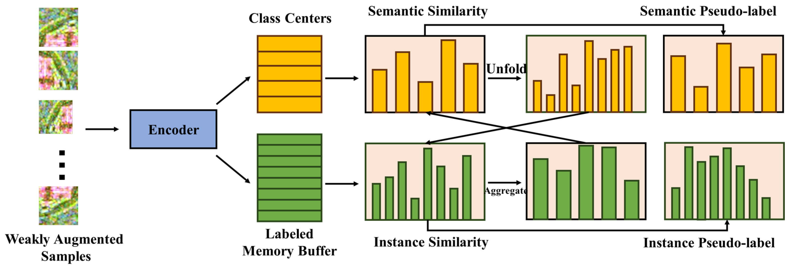
Figure 1 illustrates the five parts of the proposed framework. The first part shows the steps in the generation of representative points of superpixels. The second part shows the preliminary generation of maps by the unsupervised learning algorithm RDDMI. The third part shows how to use representative points of superpixels to improve the confidence of the maps. The three parts mentioned above constitute the method of how high-confidence pseudo-labels are generated. The fourth part is the semi-supervised algorithm SimMatch. SimMatch uses high-confidence pseudo-labels as supervision to generate pseudo-labels from unlabeled samples. Two types of losses are calculated. The fifth part is a typical use of high-confidence pseudo-labels as supervision to generate supervised predictions. In this part, the pseudo-labels and features are also stored in the memory buffer of the fourth part.

The first part presents the selection of representative points of superpixels using SLIC. The pixels in a PolSAR Pauli pseudo-color image are grouped according to the similarity of their color, brightness, and other characteristics. The generated superpixels are compact and neat like cells, and the neighborhood features are relatively easy to express. SLIC outperforms other superpixel segmentation methods in terms of contour preservation, running speed, and the compactness of the generated superpixels.

In the second part, the unsupervised learning algorithm RDDMI is used to generate preliminary pseudo-label maps. For each pixel in the PolSAR image, paired data x and $x_0$ are used as inputs for deep mutual information learning. The RDDMI generates preliminary unsupervised classification maps for the creation of pseudo-labels.

In the third part, this study refers to the contour of each superpixel to find its approximate maximum inscribed rectangle and geometric center. The shape of a single superpixel contour may be irregular, resulting in the inscribed rectangle being too small and the central representative point being inaccurate. Therefore, a certain number of contour pixels are allowed to exist in the inscribed rectangle in this process. The points corresponding to the central representative points in the maps generated by RDDMI are selected as pseudo-labels with high confidence.

In the fourth part, high-confidence pseudo-labels are used as supervision through the excellent semi-supervised algorithm SimMatch. SimMatch first uses weakly augmented views to generate semantic and instance pseudo-labels and calculates their similarity through the class center and label embedding. Then, these two similarities are fused through expansion and aggregation operations. The strongly augmented view is used to generate predictions and feature similarities. The semantic pseudo-labels and instance pseudo-labels have instance pseudo-labels and semantic pseudo-labels, respectively. Finally, the unsupervised loss $L_u$ and input loss $L_{in}$ are calculated by the predictions and similarities.

The fifth part is the process of calculating the supervision loss. The high-confidence pseudo-labels mentioned above are used as supervision. “Labels” and feature embeddings of high-confidence pseudo-label samples are stored in a labeled memory buffer.

Figure 1 shows the entire process of the algorithm proposed in this paper. First, RDDMI unsupervised learning classification is used to obtain primary pseudo-labels that contain pseudo-supervision information. Second, the PolSAR image is segmented by SLIC, and the geometric centers of the approximate maximum inscribed rectangles of superpixels are calculated. The centers are combined with the primary pseudo-label to extract high-confidence pseudo-labels. Third, the pseudo-labels are used for classification tasks through the semi-supervised algorithm SimMatch. In SimMatch, the memory buffer stores the features obtained from high-confidence pseudo-labels and performs similarity matching with the prediction results of unlabeled data to obtain more accurate results. Finally, SimMatch uses supervised loss $L_s$, unsupervised loss $L_u$, and consistency regularization loss $L_{in}$ to jointly form the overall loss function. The generalization ability and the performance of the model are guaranteed.

2.1. Method of Obtaining Pseudo-Labels

The method of obtaining pseudo-labels mainly includes three parts: (1) Using the RDDMI algorithm to generate pseudo-labels with low confidence; (2) using the SLIC algorithm to segment PolSAR images and calculate the representative points of each superpixel; (3) combining representative points of superpixels with low-confidence maps to extract high-confidence pseudo-labels.

2.1.1. RDDMI

The RDDMI algorithm represents a significant advancement in the realm of unsupervised learning for PolSAR image classification. In RDDMI, an end-to-end convolutional long short-term memory (ConvLSTM) network was used. The data processing workflow is simplified. The deep mutual information associated with various polarization directions (POAs) in the rotation domain of the polarization coherence matrix is effectively learned. RDDMI has good classification accuracy and rapid processing capabilities, allowing for the swift generation of accurate pseudo-labels for subsequent analysis. ConvLSTM has taken the place of LSTM’s [38] fully connected gate layers with convolutional layers, enabling it to process sequence data with spatial information.

The architecture of the RDDMI network initiates with two ConvLSTM layers to extract rotational-domain features from the inputs. Next, three convolutional layers, three max-pooling layers, and two fully connected layers are applied to further refine and learn deep features. The network culminates in a softmax layer to output a one-hot vector, with the argmax function being employed to calculate the class of the sample [23].

As shown in Equation (1), the loss function includes pseudo-label loss, pseudo-graph loss, and two mutual losses based on the predicted features of x and $x_0$ information losses. RDDMI first introduces pseudo-label supervised loss, pseudo-graph supervised loss, and triple mutual information loss into DCCM [23]. The similarity matrix between samples is calculated using the predictive properties of the network. The shallow features output by the first max-pooling layer and the deep features output by the second fully connected layer are used to calculate the mutual loss of triples.

$$\underset{\mathrm{\Phi }}{min}L=L_{IIC\_MI}+\alpha \widehat{L_{PG}}+\beta \widehat{L_{PL}}+\gamma L_{TRI\_MI}$$

(1)

2.1.2. Representative Points of Superpixels

Superpixels are a group of pixels that are combined based on similar colors or low-level features. In the unsupervised classification of PolSAR images, there are common phenomena of blurred boundaries and inaccurate boundary classifications. This will affect the overall classification accuracy and lead to low overall confidence in pseudo-labels. Reference superpixel segmentation overcomes speckle noise by extracting color features. The PolSAR image is divided into several superpixels with similar color features using superpixel segmentation. The geometric center point of each superpixel is used as an accurate and representative pseudo-label point. This approach abandons a large amount of boundary information that is highly likely to be erroneous, increasing the confidence of pseudo-labels. Therefore, there is an urgent need for an accurate and fast superpixel segmentation method. In existing methods, the superpixels generated by SLIC have precise boundary adhesion and uniform regularity. SLIC requires very few parameters to be set, and by default, only the number of pre-segmented superpixels needs to be set. Therefore, this study uses SLIC to quickly segment PolSAR images into many superpixels. Then, the approximate maximum inscribed rectangle of each superpixel is calculated. This rectangle allows an appropriate number of pixels on the superpixel outline inside the rectangle to ensure that it is centered, and the largest rectangle is calculated. At this point, the center point of the rectangle can also be considered as the center point of the superpixel, which is representative. Finally, the representative points are combined with the maps generated by the RDDMI mentioned above to form a high-confidence pseudo-label.

2.2. Framework of SimMatch Semi-Supervised Learning

The extracted pseudo-labels have high confidence, but the quantity is limited. The situation at this point is similar to semi-supervised learning. A small amount of labels are used in semi-supervised learning, so a semi-supervised learning algorithm is needed to complete the remaining processing work. In [39], SimMatch was used to detect changes in PolSAR images, and the effect was significant. SimMatch is a suitable semi-supervised image classification algorithm with good performance under limited label conditions. This is a way to propagate pseudo-labels’ information to each other, and it uses the label memory buffer to achieve the isomorphic transformation of two types of similarity. SimMatch solves the problems of model overfitting and improves the reliability of the model. SimMatch effectively utilizes the idea of combining consistency regularization with pseudo-labels in FixMatch [34]. This section will first review consistency regularization and pseudo-labels and then introduce the innovation of SimMatch, which allows pseudo-label information to mutually propagate.

Firstly, the image classification problem can be defined as there being a set of labeled samples $X=\left\{(x_b,p_b):b\in (1\dots ,B)\right\}$ and unlabeled samples $u=\left\{u_b:b\in (1\dots ,\mu B)\right\}$, where $p_b$ is the label of sample $x_b$. Data augmentation is often used to improve the generalization ability of models. The weakly augmented function and strongly augmented function are defined as $T_w\left(·\right)$ and $T_s\left(·\right)$.

2.2.1. Two Methods in Semi-Supervision

Consistency regularization is frequently used in semi-supervised learning. Consistency regularization was first proposed in [40], and it requires ensuring that the same image still has similar prediction results under different perturbations. In the models in [41], the loss function is used for unlabeled samples as follows:

$$\sum _{b=1}^{\mu B}{\parallel p_{\mathrm{m}}(y\mid \mid T_w\left(u_b\right))-p_{\mathrm{m}}(y\mid \mid T_w\left(u_b\right))\parallel }_2^2$$

(2)

Here, $p_{\mathrm{m}}(y\mid x)$ is the predicted classification result of input x, and both $T_w$ and $p_{\mathrm{m}}$ are random. SimMatch uses cross-entropy loss instead of square loss.

Pseudo-labeling is also commonly used in semi-supervised learning. Pseudo-labels are obtained from the model itself. Specifically, during supervised training, the prediction with a maximum class probability higher than the threshold $\tau$ is retained. This prediction is used as the pseudo-label of the unlabeled sample. It can be expressed by the following loss function:

$$\begin{array}{c}\hfill {\displaystyle \frac{1}{\mu B}}\sum _{b=1}^{\mu B}1(max\left(p_{\mathrm{m}}(y\mid u_b)\right)\ge \tau )H({\widehat{q}}_b,p_{\mathrm{m}}(y\mid u_b))\end{array}$$

(3)

where ${\widehat{q}}_b=argmax\left(q_b\right)$. FixMatch applies $argmax$ to the prediction to generate an effective one-hot prediction. Differently, in SimMatch, a distribution alignment strategy $DA(·)$ [33] is adopted to balance the distribution of pseudo-labels, and $DA\left(p^w\right)$ is directly used as the pseudo-label to calculate the cross-entropy between the strongly augmented sample predictions $p^s$:

$${\displaystyle \frac{1}{\mu B}}\sum 1(max\left(DA\left(p^w\right)\right)>\tau )\mathrm{H}(DA\left(p^w\right),p^s)$$

(4)

2.2.2. Instance Similarity

SimMatch encourages the similarity distributions of strongly and weakly augmented views to align closely. A nonlinear head $g(·)$ representing h maps to a feature embedding ${\mathit{z}}_b=g\left({\mathit{h}}_b\right)$ is assumed. The augmented anchoring and the embeddings can be denoted by ${\mathit{z}}_b^W$ (the weakly augmented views) and ${\mathit{z}}_b^s$ (the strongly augmented views), respectively. For the $\mathit{K}$ embeddings of various weakly augmented samples $\left\{z_k:k\in (1\dots ,K)\right\}$, the similarity with ${\mathit{z}}^W$ and the $\mathit{i}$-th instance are calculated by a similarity function $sim\left(·\right)$. This is represented by the dot product between ${\mathit{L}}_2$ and the normalized vector $\mathit{sim}(\mathit{u},\mathit{v})={\mathit{u}}^T\mathit{v}///\mathit{u}//$$//\mathit{v}//$. Then, the generated similarity is processed through a softmax layer. In the generated similarity distribution, $\mathit{t}$ is used as a temperature parameter to adjust the sharpness of the distribution:

$$q_i^W={\displaystyle \frac{exp\left(sim\left({\mathit{z}}_b^W,{\mathit{z}}_i\right)/t\right)}{{\sum }_{k=1}^{K}exp\left(sim\left({\mathit{z}}_b^w,{\mathit{z}}_k\right)/t\right)}}$$

(5)

The sim $\left(z_b^s,z_k\right)$ is used to calculate the similarity between strongly augmented views ${\mathit{z}}^S$ and ${\mathit{z}}_i$ to obtain the similarity distribution:

$$q_i^s={\displaystyle \frac{exp(sim(z_b^s,z_i)/t)}{{\sum }_{k=1}^{K}exp(sim(z_b^s,z_k)/t)}}$$

(6)

2.2.3. Label Information Dissemination

The SimMatch framework also considers instance-level consistency regularization. The use of entirely unsupervised instance pseudo-labels, denoted as $q^W$, leads to a considerable waste of label information. To address this issue, SimMatch utilizes labeled information at the instance level. The interaction between semantic and instance similarity is enhanced, thereby improving the result of the generated pseudo-labels. The labeled memory buffer saves all labeled samples, as shown in Figure 2. Each ${\mathit{z}}_{\mathit{k}}$ in Equations (5) and (6) can be associated with a specific class. The vectors in $\varphi$ are regarded as center class references when the labeled samples stored in the memory buffer can be viewed as the same class. $p^w\in R^{1\times L}$ is semantic similarity and $q^w\in R^{1\times K}$ is instance similarity. Both of them are computed by using weakly augmented samples. It should be noted that the value of L is typically much smaller than that of K because each class requires at least one sample. Subsequently, $q^W$ is calibrated by expanding $p^w$ (referred to as $p^{unfold}$). Aligning the semantic similarities embedded within labels leads to the following results:

$$p_i^{unfold}=p_j^w,whereclass\left(q_j^w\right)=class\left(p_i^w\right)$$

(7)

In Equation (7), $class(·)$ can return the basic truth class. The $class\left(q_j^w\right)$ indicates the label of the jth element in the memory buffer and represents the ith class. Then, the calibrated instance pseudo-labels are regenerated by scaling $q^W$ through $p^{unfold}$ and can be expressed as

$${\widehat{q}}_i={\displaystyle \frac{q_i^w{p}_i^{unfold}}{{\sum }_{k=1}^K{q}_k^w{p}_k^{unfold}}}$$

(8)

The old labels $q^W$ will be updated to the pseudo-labels $\widehat{q}$ of the instance. At the same time, q will be aggregated into an L-dimensional space. The instance similarity is combined with the semantic similarity, represented as $q^{agg}$. Then, the instance similarity is summed to achieve the sharing of the same ground-truth labels:

$$q_{i-m}^{agg}=\sum _{j=0}^{K}1(class\left(p_i^w\right)=class\left(q_j^w\right))q_j^w$$

(9)

The semantic pseudo-labels will be updated by using $q^{agg}$ to smooth $p^W$:

$${\widehat{p}}_i=\alpha p_i^w+(1-a)q_i^{agg}$$

(10)

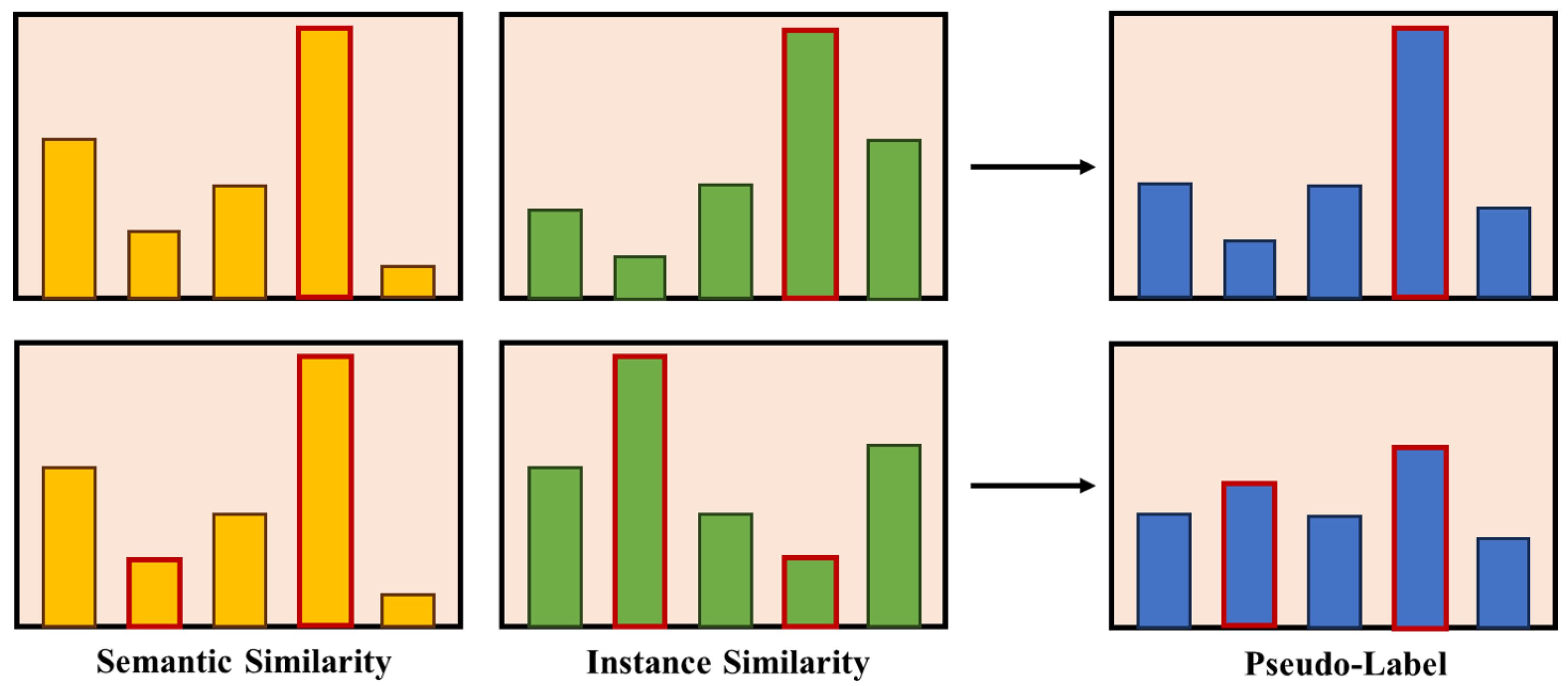
In Equation (10), $\alpha$ is the hyperparameter that controls the instance information and semantic weight. The pseudo-label p will contain semantic-level information and q will contain instance-level information. Similarly, the old value, $p_i^W$, will be replaced with the adjusted semantic pseudo-label. If the two are not close, the histogram will be flatter. As shown in Figure 3, if these two similarities are very close, it means that the predictions of the two similarities’ distributions are consistent, and the histogram will be sharp.

2.2.4. Memory Buffer

SimMatch stores ground-truth labels and feature embeddings of labeled samples in a memory buffer. Specifically, it delineates a label memory buffer, denoted as $P_l\in R^{N\times 1}$, and a feature memory buffer, referred to as $P_f\in R^{N\times D}$, where D represents the embedding size and N represents the amounts of labeled samples. For the label memory buffer, each label only stores one scalar. Aggregation and unfolding operations are implemented through functions provided by a deep learning library [35]. Given the variance in buffer sizes, SimMatch employs two distinct implementations. When N is large, the memory buffer is represented as $M_s$ and $M_t$ using the student–teacher framework [42]. The labeled samples and strongly augmented samples are directed to $M_t$, while weakly augmented samples are input into $M_t$ to generate pseudo-labels. The updating process for $M_t$ is as follows:

$$M_t\leftarrow (1-m)M_s+m{M}_t$$

(11)

When N is small, a time integration strategy [43] is used to smooth the feature embeddings, and this can be defined as

$$Y_t\leftarrow (1-m)Y_t+m{Y}_{t-1}$$

(12)

In this case, the same encoder will receive all samples.

2.3. Loss

In SimMatch, the feature information $\mathit{h}=f\left(T\right(x\left)\right)$ of weakly augmented labeled samples $x=\{x_b:b\in (1,\dots ,B)\}$ is extracted by encoder $F(·)$ of the convolutional neural network. The fully connected prediction head $\varphi (·)$ is used to calculate the semantic similarity $p=\varphi \left(\mathit{h}\right)$ and the supervised classification loss as follows:

$$L_s={\displaystyle \frac{1}{B}}\Sigma H(y,p)$$

(13)

Applying the weakly augmented function $T_w\left(·\right)$ and the strongly augmented function $T_s\left(·\right)$ to unlabeled samples to obtain weakly augmented samples $p^w$ and strongly augmented samples $p^s$, $DA(·)$ is a distribution alignment method used to balance the distribution of pseudo-labels [33]. Then, it is necessary to keep the moving average of $p_{avg}^w$ constant and use $Normalize(p^w/p_{avg}^w)$ to adjust the current $p^w$ [44]. $DA\left(p^w\right)$ is used directly as pseudo-labels. The cross-entropy between $p^w$(pseudo-label) and $p^s$(semantic-similarity) is used to define unsupervised loss:

$$L_u={\displaystyle \frac{1}{\mu B}}\sum 1(max\left(DA\left(p^w\right)\right)>\tau )H(DA\left(p^w\right),p^s)$$

(14)

By minimizing the difference between $q^w$ and $q^s$, consistency regularization can be achieved, and this is represented by the cross-entropy as

$$L_{in}={\displaystyle \frac{1}{\mu B}}\sum H(q^w,q^s)$$

(15)

The overall loss function of SimMatch is:

$$L_{overall}=L_s+{\lambda }_u{L}_u+{\lambda }_{in}{L}_{in}$$

(16)

3. Experiment

To validate the feasibility of the proposed method, multiple comparative experiments were conducted on three PolSAR datasets. Four PolSAR image classification methods, which were the classic unsupervised method, the Wishart cluster, the deep learning-based method RDDMI, and the traditional supervised random forest (RF) method, were used to compare with the proposed method. The supervised training of Random Forest (RF) uses 25,000 randomly selected labeled samples for each PolSAR datum. During this process, the input data are 15 × 15 neighborhood window data, which is the same size as the neighborhood window used in the proposed method. At the same time, the same normalization method is used for data processing to ensure data consistency.

The experimental results were evaluated using the overall accuracy (OA), kappa, precision, recall, and F1 score.

The proportion of overall correct predictions is calculated by OA. The kappa was used for unbalanced samples. The precision reflects the proportion of samples belonging to a certain class among the samples predicted as that class by the model. Recall is defined as the proportion of samples that are correctly identified by the model as belonging to a certain class. The F1 score is used to comprehensively measure the precision and recall of the model.

3.1. Datasets

This section introduces three real PolSAR image data. The data details are shown in the

Table 1. Information of the three datasets.

Parameter	RS-2 Flevoland	AIRSAR Flevoland	RS-2 Wuhan
Sensor	RADARSAT-2	NASA/JPL AIRSAR	RADARSAT-2
Band	C	L	C
Imaging Area	Flevoland	Flevoland	Wuhan
Imaging Mode	Quad-pol	∖	Quad-pol
Imaging time	2008	16 August 1989	December 2011
Spatial resolution [Range Azimuth] (m)	$12\times 8$	$6\times 12$	$12\times 8$
Image size [Range Azimuth] (pixel)	$1400\times 1200$	$750\times 1024$	$5500\times 2400$

.

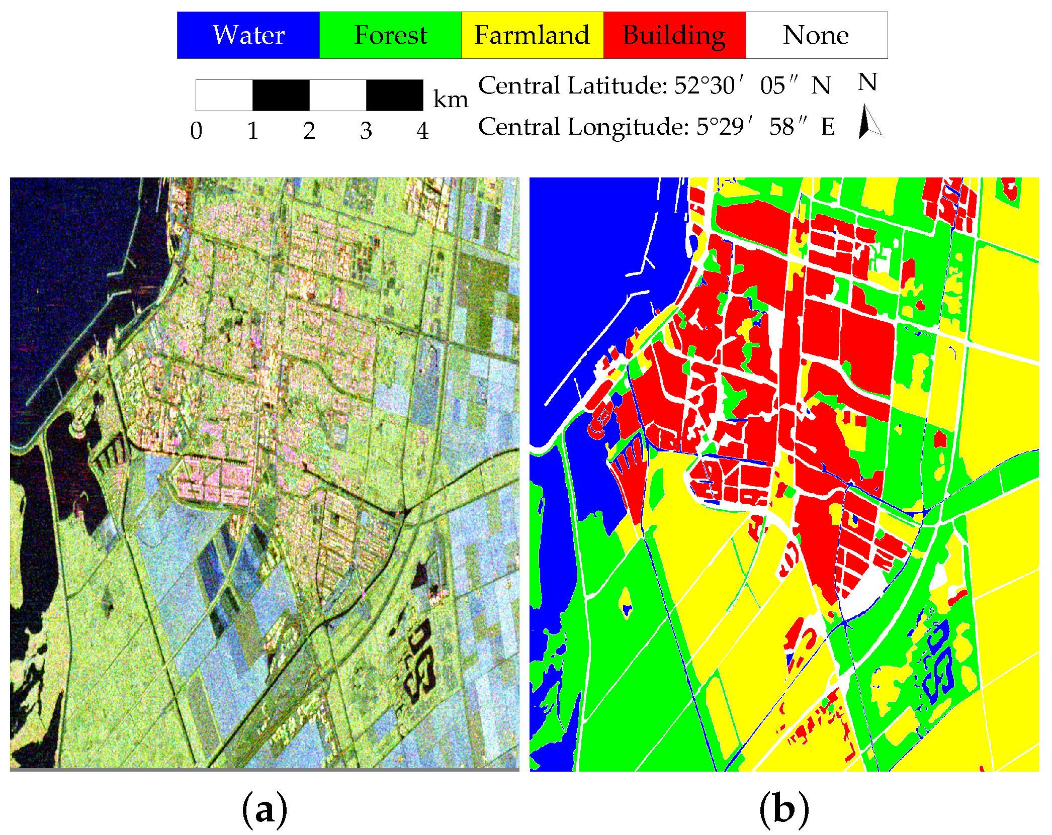
3.1.1. RADARSAT-2 Flevoland Dataset

In the field of PolSAR image classification, the RADARSAT-2 (RS-2) Flevoland dataset is widely used. This dataset has an image size of 1400 × 1200 pixels and a spatial resolution of 12 × 8 m. It covers the Flevoland region of the Netherlands and has four land cover categories: farmland, water, forests, and buildings. The Pauli pseudo-color image and the corresponding ground-truth map of the RS-2 Flevoland dataset are shown in Figure 4.

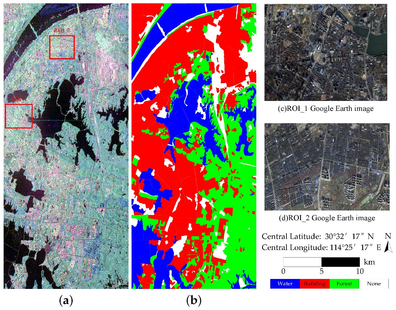
3.1.2. RADARSAT-2 Wuhan Dataset

The RS-2 Wuhan dataset covers the scene of Wuhan and was obtained using the RADARSAT-2 C-band PolSAR system in the fine quad-pol mode. The image size is 5500 × 2400 pixels. The spatial resolution is 12 × 8 m. It contains three land cover categories: water, forest, and buildings. This dataset has highly dense buildings with different orientations, which increases the difficulty of clustering. The Pauli pseudo-color image and the corresponding ground-truth map of the RS-2 Wuhan dataset are shown in Figure 5.

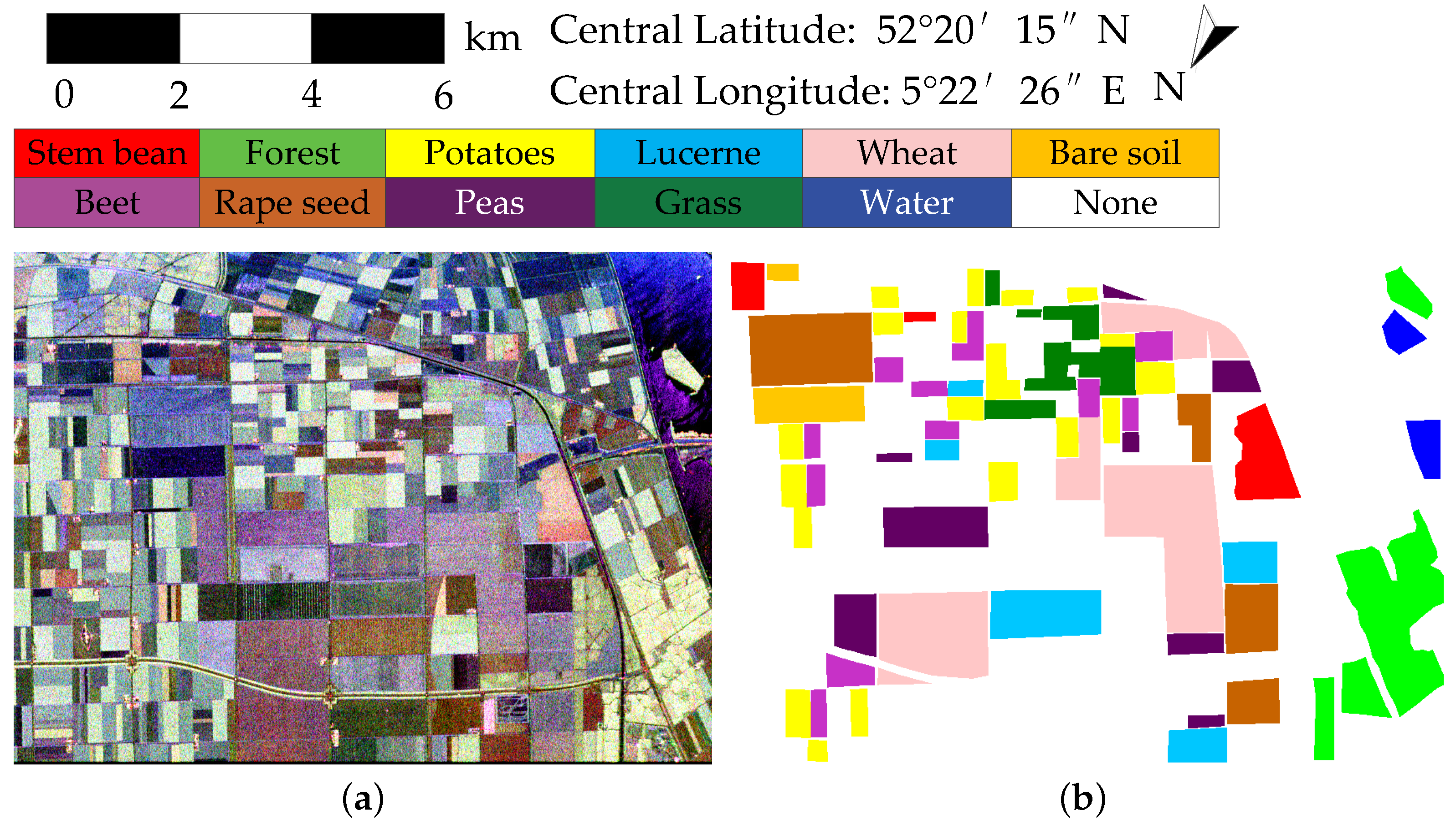
3.1.3. AIRSAR Flevoland Dataset

The AIRSAR Flevoland dataset contains four-look fully polarimetric images and was acquired by the NASA/JPL AIRSAR L-band system. This dataset also covers the scene of Flevoland, the Netherlands. The image size is 750 × 1024 pixels. The spatial resolution is 6 × 12 m. It contains 11 types of land cover, including forests, wheat, and 9 other types. The Pauli pseudo-color image and the corresponding ground-truth map of the AIRSAR Flevoland dataset are shown in Figure 6.

3.2. Results

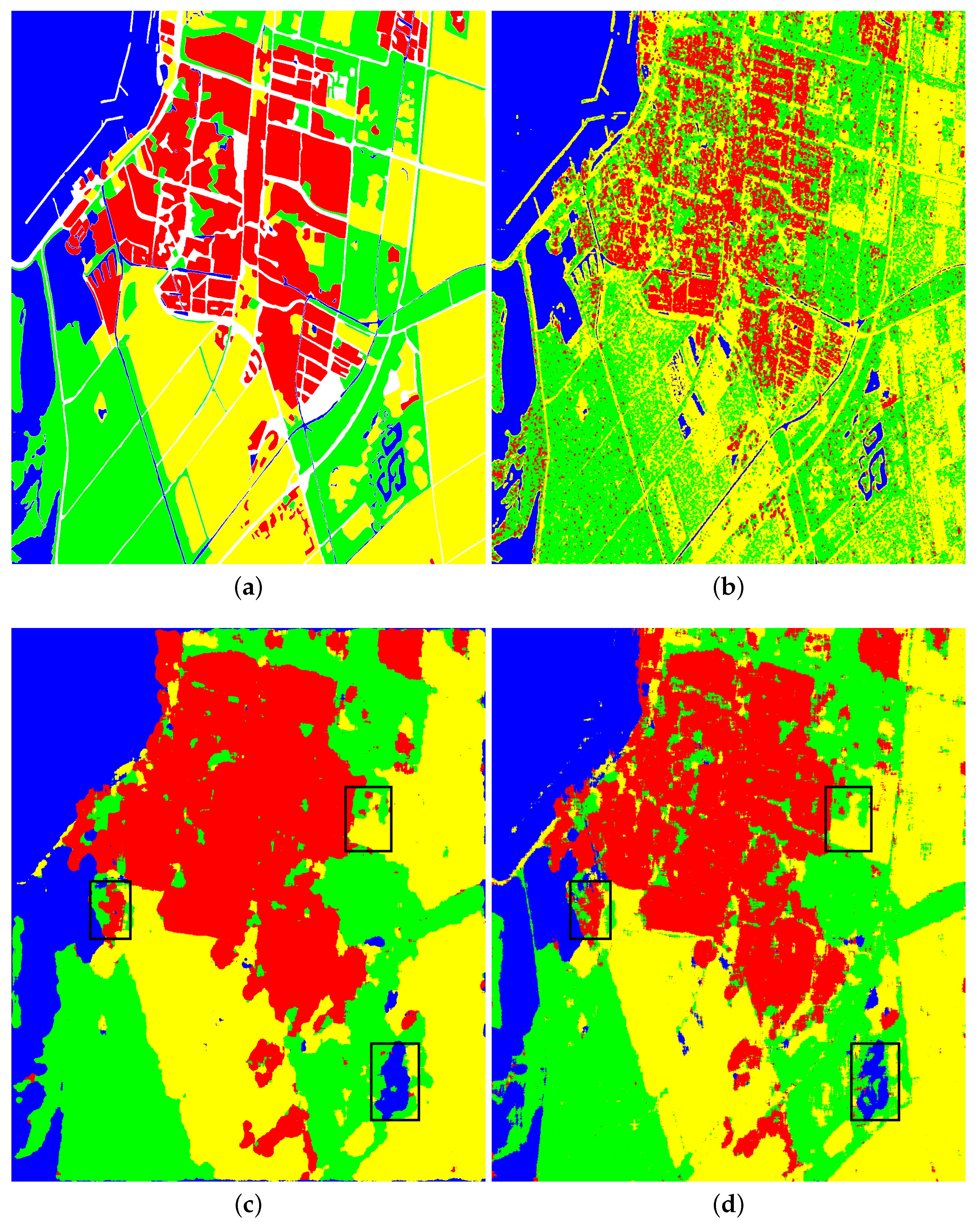
3.2.1. Results on the RS-2 Flevoland Dataset

The classification results on the RS-2 Flevoland dataset are shown in Figure 7 and

Table 2. The results of RS-2 Flevoland. The best performance is bolded.

Land Cover	Wishart	RDDMI	SP-SIM	RF
Water	90.63	92.49	93.10	95.85
Forest	77.77	82.14	86.31	87.77
Farmland	65.65	86.42	89.04	85.60
Building	55.31	94.16	91.88	82.39
OA	71.35	87.86	89.56	88.10
Kappa	0.61	0.83	0.86	0.83
precision	0.76	0.87	0.89	0.88
recall	0.72	0.89	0.90	0.88
F1	0.73	0.88	0.90	0.88

. The RS-2 Flevoland dataset contains forest and farmland types embedded in building types, and farmland types have different backscattering properties, which poses difficulties for accurate classification. Wishart performed poorly on this dataset, and a large number of buildings and farmlands were identified as forests. RDDMI showed great classification performance and improved the OA to 87.86%. However, the pixels on the boundaries were not precisely classified. The proposed SP-SIM was superior to the above methods. In particular, the boundary pixels were finely classified, as shown in the black boxes in Figure 7c,d. The building and water types were all well classified. The boundaries of farmlands were also much better than those of RDDMI. Compared with RDDMI, the accuracies of the proposed method for water, forest, and farmland were increased by 0.61%, 4.17%, and 2.62%, respectively. Finally, the OA of the SP-SIM increased by 1.70%. Meanwhile, the OA of the SP-SIM was 1.46% higher than that of supervised RF. Moreover, the precision, recall, and F1 score are all higher than those of other methods, including RF. The above analysis demonstrates the obvious performance improvement and proves that the proposed framework is efficient for unsupervised PolSAR image classification.

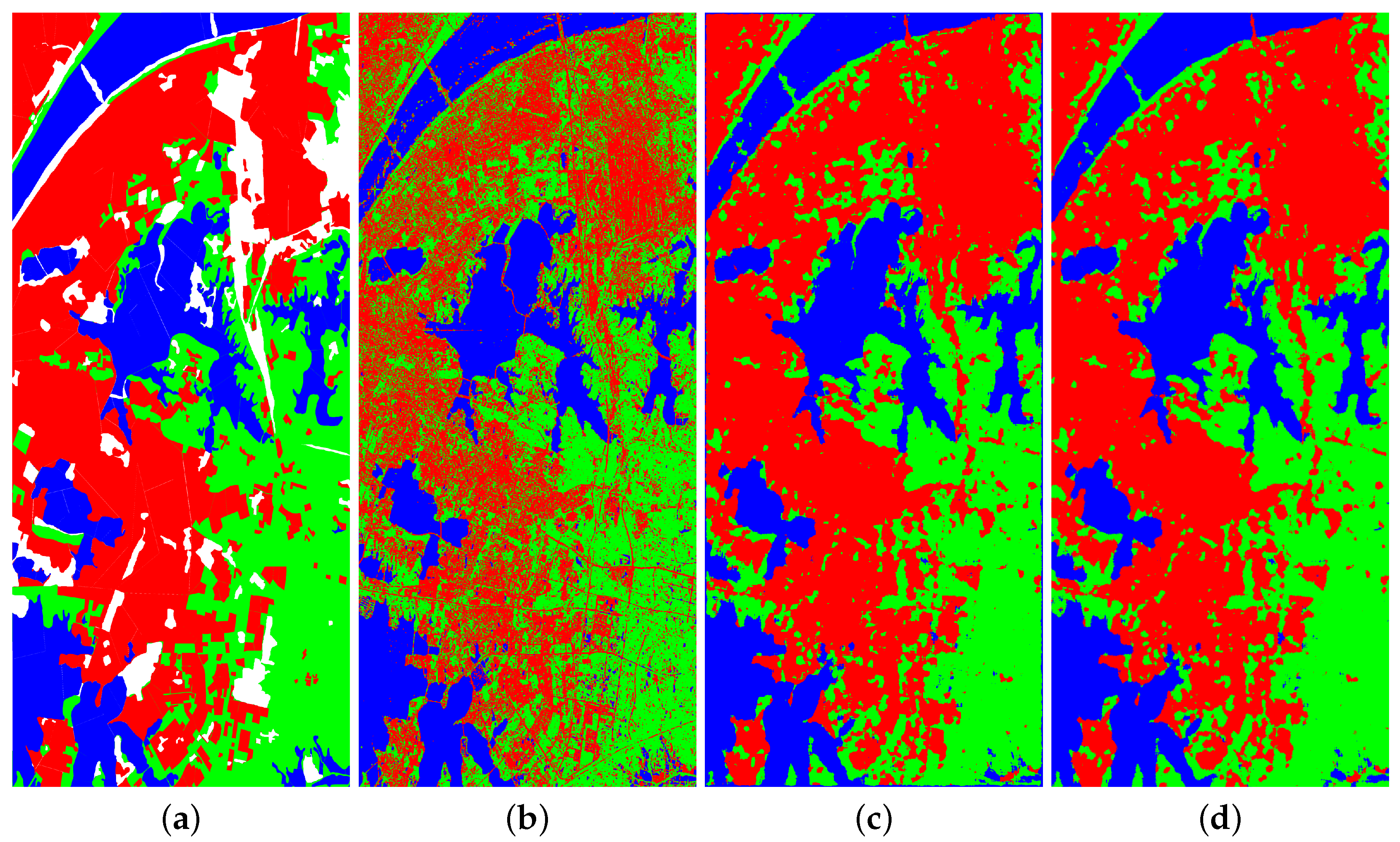
3.2.2. Results on the RS-2 Wuhan Dataset

In the RS-2 Wuhan dataset, there is a large number of buildings with different orientations, which exhibit different features in PolSAR images. It is difficult to accurately distinguish building types through unsupervised methods. Figure 8 shows the classification maps, and

Table 3. The results of the RS-2 Wuhan dataset. The best performance is bolded.

Land Cover	Wishart	RDDMI	SP-SIM	RF
Water	88.10	92.26	92.54	94.01
Forest	67.89	88.49	89.20	88.34
Building	74.02	75.83	77.71	81.44
OA	74.55	85.31	86.30	87.45
Kappa	0.60	0.77	0.79	0.80
precision	0.78	0.86	0.87	0.88
recall	0.77	0.86	0.86	0.88
F1	0.81	0.86	0.87	0.88

displays the quantitative results. RDDMI achieved very good results on this dataset, with impressive accuracy in identifying buildings. The results of the traditional Wishart cluster were not good. The OA of SP-SIM was 0.99% higher than that of RDDMI and close to that of the supervised RF method. The accuracies for all land cover types were better than those of RDDMI. The precision, recall and F1 score are all higher than those of the other methods. The experiment demonstrated the effectiveness of the proposed method on PolSAR images.

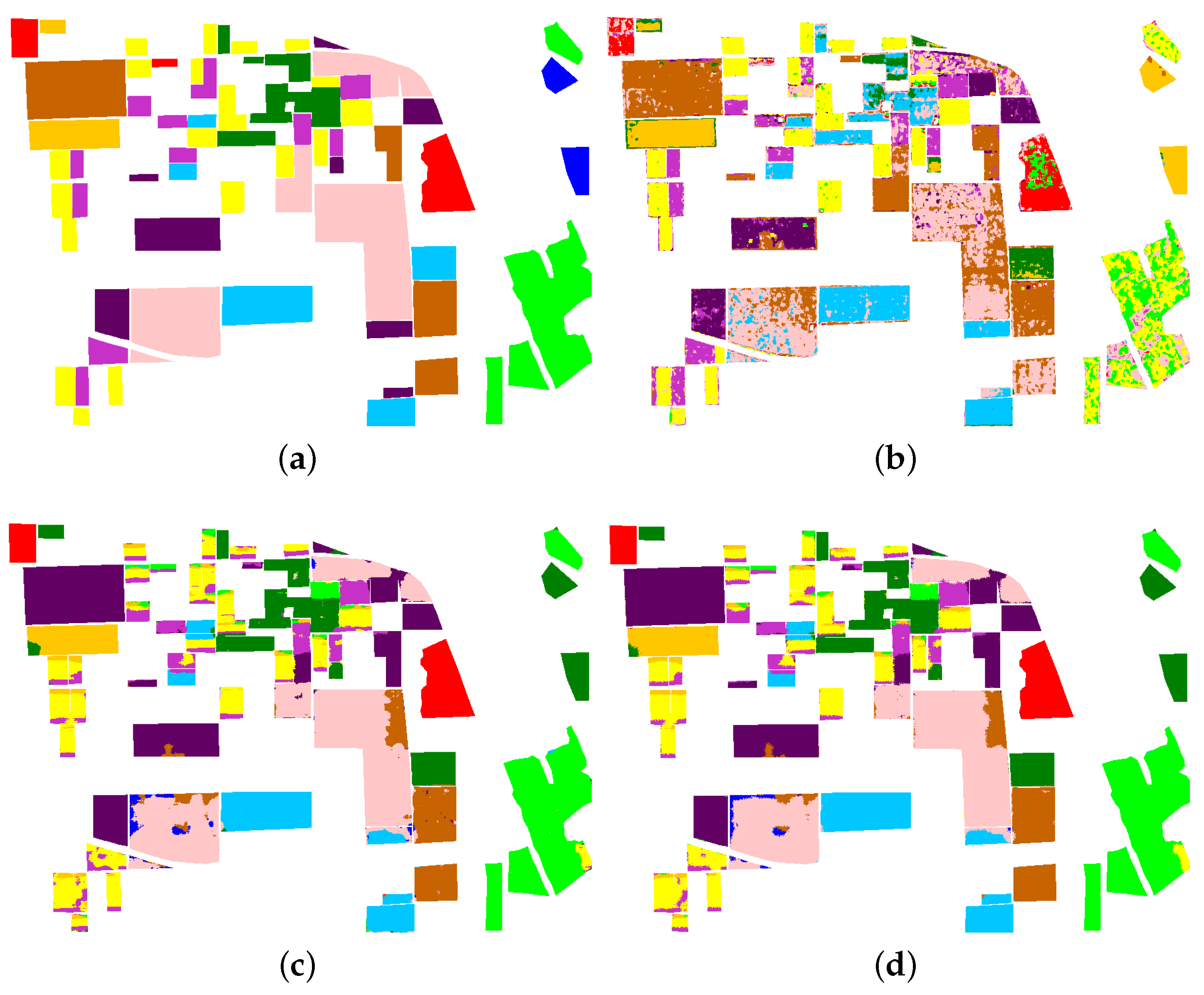
3.2.3. Results on the AIRSAR Flevoland Dataset

The AIRSAR Flevoland dataset has up to 11 categories, and the polarization properties of each category are also very complicated, which is undoubtedly a huge challenge for unsupervised classification. The backscattering properties of some land cover types have similarities in this dataset. In addition, there may be large differences in the polarization matrices observed for the same land cover type. As shown in Figure 9, the properties of water are similar to those of other categories, which will greatly affect the classification performance. The RF method can overcome these interpretation ambiguity problems to a certain extent by supervising the information. However, the unsupervised method makes it difficult to overcome this problem of interpretation ambiguity without supervised information, so the classification performance is poor. Moreover, this dataset contains many unlabeled areas; we only used labeled areas to evaluate the results.

In Figure 10 and

Table 4. The results of the AIRSAR Flevoland dataset. The best performance is bolded.

Land Cover	Wishart	RDDMI	SP-SIM	RF
Stem bean	65.15	94.88	94.68	96.69
Forest	31.13	97.19	97.46	90.18
Potatoes	87.70	65.48	68.84	89.62
Lucerne	67.49	75.78	76.85	89.17
Wheat	57.71	82.18	83.30	77.94
Bare soil	82.38	82.88	84.49	95.57
Beet	71.59	53.32	50.73	89.00
Rape seed	79.90	35.07	35.88	90.38
Peas	57.95	78.80	78.80	73.50
Grass	50.36	91.58	92.42	93.56
Water	0	0	0	99.97
OA	59.34	72.84	73.64	86.81
Kappa	0.5	0.69	0.70	0.85
precision	0.56	0.67	0.67	0.87
recall	0.56	0.69	0.69	0.90
F1	0.54	0.66	0.66	0.88

, it can be seen that Wishart could not make accurate judgments on categories with similar polarization characteristics, and RDDMI achieved better results. All methods cannot accurately classify water. This is because the backscattering properties of water are similar to those of other categories. The proposed method had a certain improvement based on RDDMI, and the OA was increased by 0.80%. Other indicators also reached an excellent level. The experiment showed that although the proposed framework was able to improve the unsupervised PolSAR classification performance, it also had its limitations. The maps of RDDMI will affect the performance of the proposed method. If the results of RDDMI are poor, the performance of the proposed method will be limited.

4. Discussion

4.1. Effect of the Unsupervised Algorithm

To study the importance of the excellent unsupervised learning results of RDDMI to the proposed method, the pseudo-labels extracted from the Wishart and DCCM classification results are used for semi-supervised classification by SimMatch. These two methods are called SLIC-Wishart and SLIC-DCCM in the table, indicating the pseudo-labels extracted by the SLIC superpixel segmentation method. The results are shown in the

Table 5. The results of the RS-2 Flevoland dataset. The best performance is bolded.

Land Cover	Wishart	SLIC-Wishart	DCCM	SLIC-DCCM	SP-SIM
Water	90.63	92.55	93.98	94.52	93.10
Forest	77.77	80.78	76.81	83.87	86.31
Farmland	65.65	67.00	83.74	86.78	89.04
Building	55.31	59.63	94.83	92.11	91.88
OA	71.35	73.89	85.87	88.40	89.56
Kappa	0.61	0.64	0.81	0.84	0.86
precision	0.76	0.78	0.86	0.88	0.89
recall	0.72	0.75	0.87	0.89	0.90
F1	0.73	0.76	0.86	0.88	0.90

,

Table 6. The results of the RS-2 Wuhan dataset. The best performance is bolded.

Land Cover	Wishart	SLIC-Wishart	DCCM	SLIC-DCCM	SP-SIM
Water	88.10	89.37	97.19	97.16	92.54
Forest	67.89	76.48	58.15	79.52	89.20
Building	74.02	76.26	75.01	63.23	77.71
OA	74.55	79.38	72.63	76.33	86.30
Kappa	0.60	0.68	0.59	0.64	0.79
precision	0.78	0.81	0.74	0.78	0.87
recall	0.77	0.81	0.77	0.80	0.86
F1	0.77	0.81	0.73	0.77	0.87

and

Table 7. The results of the AIRSAR Flevoland dataset. The best performance is bolded.

Land Cover	Wishart	SLIC-Wishart	DCCM	SLIC-DCCM	SP-SIM
Stem bean	65.15	76.69	69.51	69.62	94.68
Forest	31.13	25.03	98.30	98.37	97.46
Potatoes	87.70	92.02	43.12	42.67	68.84
Lucerne	67.49	73.61	78.45	78.73	76.85
Wheat	57.71	60.55	34.67	34.73	83.30
Bare soil	82.38	91.82	92.44	92.82	84.49
Beet	71.59	79.81	2.35	2.19	50.73
Rape seed	79.90	82.43	56.78	56.81	35.88
Peas	57.95	62.96	74.35	74.35	78.80
Grass	50.36	18.62	17.55	72.99	92.42
Water	0	0	0	0	0
OA	59.34	63.25	60.62	56.43	73.64
Kappa	0.54	0.58	0.55	0.52	0.70
precision	0.57	0.60	0.58	0.58	0.67
recall	0.56	0.60	0.57	0.57	0.69
F1	0.54	0.57	0.53	0.53	0.66

.

In the RS2-Flevoland and RS2-Wuhan datasets, high-confidence pseudo-label extraction was performed on the Wishart and DCCM results. The classification results of SLIC-Wishart and SLIC-DCCM were not as good as those obtained by using RDDMI for pseudo-label extraction as proposed in this paper. However, compared to the results of Wishart and DCCM, there was a significant improvement. All indicators in the results were improved to an extent, proving that the method of extracting high-confidence pseudo-labels through superpixels is feasible.

In the AIRSAR Flevoland dataset, the combination of RDDMI high-confidence pseudo-labels and SimMatch adopted in this paper has results far superior to those of extracting pseudo-labels with Wishart and DCCM, proving the viability of the scheme proposed above. The high-confidence pseudo-labels extracted by using the results of RDDMI still have the best performance, as mentioned above. The result of SLIC-Wishart is also better than that of Wishart. It can be inferred that the quality of high-confidence pseudo-labels extracted from unsupervised results using superpixels depends on the initial unsupervised classification results. The high-performance unsupervised classification results of RDDMI are very important to the results of this framework.

This raises a limitation: the method proposed requires high-quality initial unsupervised classification maps, which limits the quality of unsupervised classification results. The extraction of pseudo-labels through superpixel segmentation can only provide limited improvement for unsupervised algorithms with poor results. Further research is needed to address this limitation.

4.2. Effect of the Semi-Supervised Algorithm

The method proposed in this paper can extract large amounts of high-confidence pseudo-labels, which are directly used as supervision information. The supervision information can be used in the semi-supervised algorithm in the proposed method and can also be used in a supervised classification method. In this study, 25,000 superpixels were used to extract high-confidence pseudo-labels and conduct classification experiments on three datasets using the supervised learning classification method VGG-16 as a comparison. The 20,287 pseudo-label samples of the RS-2 Flevoland dataset were used. As shown in

Table 8. Performance evaluation of VGG-16 and SP-SIM on the RS-2 Flevoland dataset. The best performance is bolded.

Land Cover	VGG-16, 20,287 Samples	SP-SIM, 20,287 Sample
Water	92.06	93.10
Forest	83.56	86.31
Farmland	86.54	89.04
Building	91.75	91.88
OA	87.73	89.56
Kappa	0.83	0.86
precision	0.88	0.89
recall	0.88	0.90
F1	0.88	0.90

, the proposed semi-supervised method SP-SIM had an accuracy that was 1.83% higher than that of the supervised method, VGG-16, and the accuracies of each class were higher than those of VGG-16. Moreover, other indicators of SP-SIM are all superior to VGG-16. Although the number of pseudo-labeled samples was large, the effectiveness of using pseudo-labels as supervision information to directly train supervised models was not good. The semi-supervised classification method can effectively improve PolSAR image classification performance by combining pseudo-labeled samples and unlabeled samples.

In the other two datasets, it was also reflected that even with a large number of pseudo-labeled samples, the performance of semi-supervised methods was better than that of supervised methods; 20,127 pseudo-labeled samples were used to train classification models on the RS-2 Wuhan dataset. As shown in

Table 9. Performance evaluation of VGG-16 and SP-SIM on the RS-2 Wuhan dataset. The best performance is bolded.

Land Cover	VGG-16, 20,127 Samples	SP-SIM, 20,127 Sample
Water	91.38	92.54
Farmland	89.07	89.20
Building	77.38	77.71
OA	85.86	86.30
Kappa	0.78	0.79
precision	0.87	0.87
recall	0.86	0.86
F1	0.86	0.87

, the OA of SP-SIM was 0.44% higher than that of the supervised method, VGG-16, and the accuracies of all land cover types were all higher. In the AIRSAR Flevoland dataset, due to the large number of unrecognized regions, the number of pseudo-label samples was 5244, which was lower than that in the RS-2 Flevoland and RS-2 Wuhan datasets. However, under the same conditions, the OA of the proposed method was still 0.61% higher than that of the supervised method, as shown in

Table 10. Performance evaluation of VGG-16 and SP-SIM on the AIRSAR Flevoland dataset. The best performance is bolded.

Land Cover	VGG-16, 5244 Samples	SP-SIM, 5244 Samples
Stem bean	94.75	94.68
Forest	96.82	97.46
Potatoes	70.96	68.84
Lucerne	76.49	76.85
Wheat	81.74	83.30
Bare soil	82.75	84.49
Beet	49.50	50.73
Rape seed	35.56	35.88
Peas	78.49	78.80
Grass	89.25	92.42
Water	0	0
OA	73.03	73.64
Kappa	0.69	0.70
precision	0.67	0.67
recall	0.69	0.69
F1	0.66	0.66

.

The performance of the supervised classification method was not as good as that in semi-supervised learning methods with the same number of high-confidence pseudo-labels. Even with a large number of pseudo-labeled samples, the semi-supervised learning method outperformed the supervised learning method in terms of classification accuracy on the three datasets. This experiment’s results indicated that semi-supervised learning combined with unlabeled samples allows the more effective utilization of high-confidence pseudo-labeled samples to improve classification performance.

4.3. Effect of the Number of Superpixels

The proposed method utilizes superpixel segmentation. As the number of over-segmented superpixels increases, the number of high-confidence pseudo-label samples for unsupervised classification also increases. In this section, the impact of the number of superpixels in SLIC on classification performance is discussed. For each dataset, 6000 superpixels and 25000 superpixels were used to extract high-confidence pseudo-labels, and then 3730 and 20,287 high-confidence pseudo-labeled samples were obtained in the RS-2 Flevoland dataset. As shown in

Table 11. The results of 3730 and 20,287 pseudo-labeled samples on the RS-2 Flevoland dataset. The best performance is bolded.

Land Cover	3730 Samples	20,287 Samples
Water	92.58	93.10
Forest	83.29	86.31
Farmland	88.68	89.04
Building	92.69	91.89
OA	88.65	89.56
Kappa	0.85	0.86
precise	0.88	0.89
recall	0.89	0.90
F1	0.89	0.90

, the accuracy was increased by 0.91%. The increased number of pseudo-labeled samples further improved the classification performance. However, when the number of pseudo-labels reached a certain level, the accuracy improvement tended to stabilize.

In the AIRSAR Flevoland dataset, 953 and 5244 high-confidence pseudo-labeled samples were extracted from the superpixels. The classification results are shown in

Table 12. The results of 935 and 5244 pseudo-labeled samples on the AIRSAR Flevoland dataset. The best performance is bolded.

Land Cover	935 Samples	5244 Samples
Stem bean	94.75	94.68
Forest	98.18	97.46
Potatoes	65.04	68.84
Lucerne	77.57	76.85
Wheat	81.51	83.30
Bare soil	85.95	84.49
Beet	55.57	50.73
Rape seed	34.28	35.88
Peas	78.86	78.80
Grass	92.66	92.42
Water	0	0
OA	73.13	73.64
Kappa	0.70	0.70
precision	0.67	0.67
recall	0.69	0.69
F1	0.66	0.66

. The OA was improved by 0.51% with more pseudo-labeled samples. Other indicators are also better.

The impact of this number of pseudo-labels was even more limited in the RS-2 Wuhan dataset, with an accuracy improvement of only 0.29% for 20,127 pseudo-labeled samples compared with 5358 samples. The classification results are shown in

Table 13. The results of 5358 and 20,127 pseudo-labeled samples on the RS-2 Wuhan dataset. The best performance is bolded.

Land Cover	5358 Samples	20,127 Samples
Water	82.61	92.54
Farmland	89.31	89.20
Building	76.61	77.71
OA	86.01	86.30
Kappa	0.78	0.79
precision	0.87	0.87
recall	0.86	0.86
F1	0.86	0.87

.

Through the experiments on the three different datasets, it was shown that an increase in the number of superpixels leads to an increase in the number of high-confidence pseudo-labels, thereby improving classification performance to a certain extent. However, when the number of pseudo-labels reaches a certain level, the improvement in accuracy gradually stabilizes.

4.4. Hardware Environment and Runtime

The detailed information on the hardware platform used for this paper is shown in

Table 14. Hardware environment.

Name	Configuration Information
System	Windows11
Development Language	Python3.8
Framework	Pytorch 1.13.0 + cuda 11.6
GPU	NIVIDIA RTX A4000
CPU	Intel Core i7-11700
Memory	32 G

.

Table 15. The training and inference time of RS-2 Flevoland. The size of RS-2 Flevoland is 1200 × 1400 pixels, and 20,287 labeled samples are used.

Method	Train Time	Inference Time	Total Time
Wishart	10 s	10 s	20 s
DCCM	2 days	5 min	2 days + 5 min
RDDMI	2 days	5 min	2 days + 5 min
SimMatch	1.5 days	15 min	1.5 days + 15 min
SP-SIM	3.5 days	20 min	3.5 days + 20 min

shows the training time and inference time of five different methods on the RS-2 Flevoland dataset. Different datasets have different image sizes, so the time consumption is a little different. Since the method proposed is based on the results of preliminary unsupervised classification, it will inevitably consume more time. The additionally consumed time is the training and inference time required by the semi-supervised method SimMatch. The running speed is limited by the performance of the hardware platform. Improving the hardware platform with better performance can effectively reduce the time of training and inference. Therefore, the proposed method is acceptable in terms of time.

5. Conclusions

This study proposes a framework for the unsupervised classification of PolSAR images based on superpixel segmentation and a semi-supervised algorithm. The SLIC superpixel segmentation method and unsupervised classification maps from RDDMI are used to extract high-confidence pseudo-labeled samples. The semi-supervised method SimMatch is used to train with the high-confidence pseudo-labeled samples and unlabeled data to generate the final classification results. The proposed method was tested on three PolSAR image datasets and achieved great performance. The four evaluation indicators showed that the proposed method outperformed the state-of-the-art unsupervised classification method, RDDMI. SP-SIM has significant effectiveness for unsupervised PolSAR image classification.