Article

Deep Ensemble Remote Sensing Scene Classification via Category Distribution Association

1
Xi’an Research Institute of High Technology, Xi’an 710025, China
2
School of Artificial Intelligence, Optics and Electronics (iOPEN), Northwestern Polytechnical University, Xi’an 710072, China
3
School of Mathematica Sciences, Dalian University of Technology, Dalian 116024, China
*
Author to whom correspondence should be addressed.
These authors contributed equally to this work.
Remote Sens. 2024, 16(21), 4084; https://doi.org/10.3390/rs16214084
Submission received: 19 September 2024 / Revised: 25 October 2024 / Accepted: 27 October 2024 / Published: 1 November 2024

Abstract

:
Recently, deep learning models have been successfully and widely applied in the field of remote sensing scene classification. But, the existing deep models largely overlook the distinct learning difficulties associated with discriminating different pairs of scenes. Consequently, leveraging the relationships within category distributions and employing ensemble learning algorithms hold considerable potential in addressing these issues. In this paper, we propose a category-distribution-associated deep ensemble learning model that pays more attention to instances that are difficult to identify between similar scenes. The core idea is to utilize the degree of difficulty between categories to guide model learning, which is primarily divided into two modules: category distribution information extraction and scene classification. This method employs an autoencoder to capture distinct scene distributions within the samples and constructs a similarity matrix based on the discrepancies between distributions. Subsequently, the scene classification module adopts a stacking ensemble framework, where the base layer utilizes various neural networks to capture sample representations from shallow to deep levels. The meta layer incorporates a novel multiclass boosting algorithm that integrates sample distribution and representations of information to discriminate scenes. Exhaustive empirical evaluations on remote sensing scene benchmarks demonstrate the effectiveness and superiority of our proposed method over the state-of-the-art approaches.

Graphical Abstract

1. Introduction

Remote sensing scene classification [1,2,3,4,5,6,7,8] serves as a fundamental task in the realm of intelligent interpretation of remote sensing data, with the aim of extracting high-level semantic information from scene images and assigning them to specific scene categories. The goal is to develop models that can automatically recognize and distinguish objects or patterns within scenes [9] to provide valuable insights and decision support for various practical applications, including environmental monitoring, land cover monitoring, and natural resource management. The emergence of deep neural network models has led to significant advancements in scene classification [10]. Compared to traditional handcrafted features, deep neural network models are capable of extracting higher-level and more abstract feature information from raw pixel-level data, thereby enhancing the accuracy of scene classification [11]. However, deep neural network models also face several bottlenecks and challenges. They demand copious amounts of annotated data, computational resources, and storage for large-scale models [12], and they frequently grapple with overfitting during the training process [4,13]. In this context, the principles of ensemble learning and the utilization of category distributions offer alternative approaches to enhance the performance of deep learning models [14,15,16].
Indeed, ensemble learning [17] is commonly employed to overcome the aforementioned challenges and enhance the overall performance and generalization ability of deep learning models [14,18]. Specifically, ensemble learning is considered an effective approach in the field of machine learning, which aims to achieve better performance by combining multiple algorithmic models (base learners). Based on the optimization target and organizational form, ensemble learning algorithms can be categorized into three major types: bagging [17], boosting [19], and stacking [20,21]. Bagging (bootstrap aggregating) involves constructing multiple independent base learners by performing bootstrap sampling on the training dataset. The predictions of these base learners are then averaged or aggregated through voting to achieve ensemble integration. Boosting [19] is a sequential training process that builds a series of base learners, with each subsequent learner adjusted based on the performance of the previous one. Stacking [20] entails training multiple base learners and utilizing their prediction results as inputs to train a meta-learner, which is responsible for making the final predictions. According to theory [14], the effectiveness of ensemble learning derives from the reductions in both model variance and prediction bias. However, it also presents several limitations. Ensemble learning involves complex model training processes, and its computational complexity is high. The performance of ensemble learning relies on the diversity of the base learners: if the base classifiers are highly correlated, ensemble learning may not perform well [22].
In addition to the aforementioned challenges and bottlenecks, most scene classification models often overlook the inherent associations among different category distributions of scenes, treating all samples with equal attention. However, when dealing with samples from similar scenes, there are often samples that are difficult to differentiate. In these cases, it is crucial to pay more attention to the samples that lie between these difficult-to-separate classes [15]. These challenging samples, which are often located near the decision boundary, carry valuable information for improving a model’s performance. By focusing on these samples and giving them greater consideration during the training process, it is possible to enhance a model’s ability to handle complex regions and improve its discriminative power [23].
In this paper, addressing the aforementioned issues, we propose an ensemble scene classification method that is driven by category distribution associations and is primarily divided into two modules: category distribution information extraction and scene classification. The category distribution information extraction module aims to calculate the similarity among different class distributions and utilize this similarity to guide the classification process. The scene classification module employs stacking ensemble learning algorithms to integrate different convolutional neural network (CNN) models, thereby enhancing classification accuracy. Furthermore, within the meta layer of the stacking ensemble, a novel multiclass AdBoost method is employed to enhance the attention of the model on samples that are susceptible to misclassification within similar scenes. This approach facilitates the establishment of distinct decision boundaries for accurate classification.
The framework of the model is illustrated in Figure 1, which presents the steps and components of the model. The proposed framework is innovative as it integrates various modules by extracting the similarities between scene category distributions through the category information module. This is combined with the novel multiclass AdBoost method introduced in this paper, which enables the model to focus more on samples that are more challenging to distinguish in scene classification.
Our main contributions can be summarized as follows:
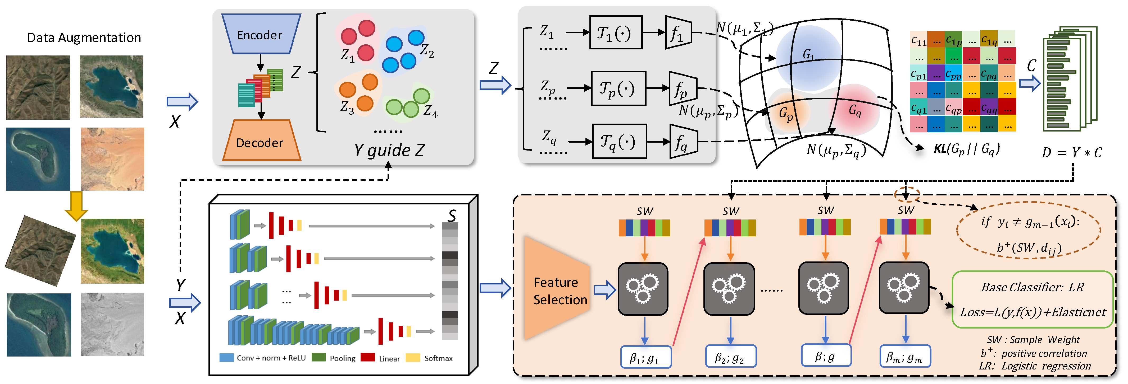
In the category distribution information extraction module, we assume that the instance distributions between the scene categories follow Gaussian distributions. By leveraging the KL divergence, we ensure that the severity of misclassification from one category to another is different from the severity in the reverse direction. This ensures that the algorithm can capture the asymmetric fitting between different category distributions, thereby enabling more accurate classification decisions.
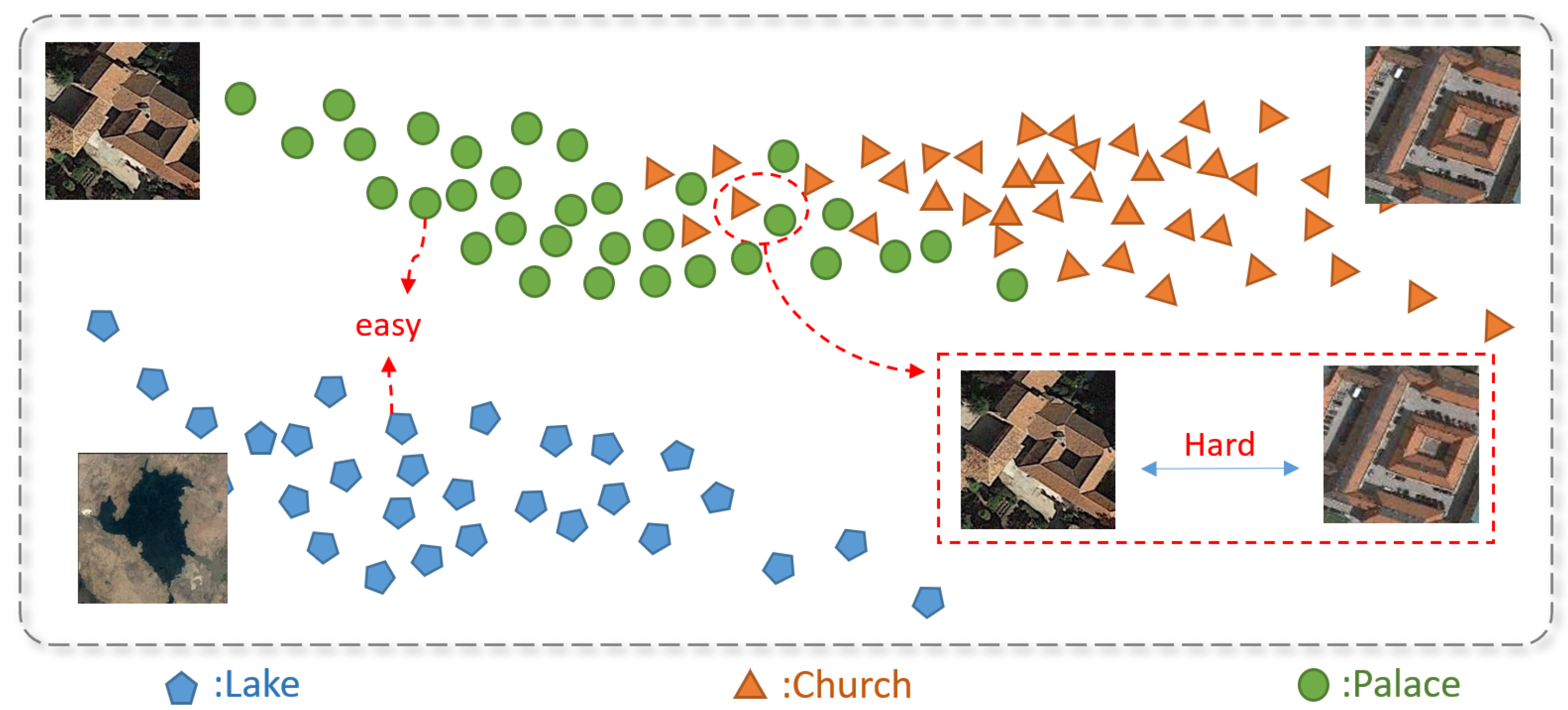
In the scene classification module, in the base layer of stacking, we aggregate the soft label outputs from multiple CNN models, allowing the model to effectively capture a broader range of information. In the meta layer of stacking, we propose a novel boosting approach. By introducing similarity among different scene distributions to adjust the instance weights, our algorithm pays more attention to difficult-to-separate category pairs.
Through exhaustive experimentation on remote sensing scene benchmarks, our proposed model demonstrates an enhancement in classification performance compared with previous methods. The effectiveness of the model components and theories was demonstrated through ablation experiments and parameter sensitivity experiments.

2. Related Studies

In this section, we review some existing work on scene classification and ensemble learning approaches.
Scene Classification: In the field of scene classification, handcrafted feature models [24] are some of the earliest and widely adopted approaches. Among them, local features such as scale-invariant feature transform (SIFT)  [25] and histogram of oriented gradients (HOG)  [26] focus on capturing distinctive local patterns and gradients within scene images. Global features such as texture descriptors and color histograms provide valuable information for discriminating different scene categories. Recently, deep neural feature models have been widely used in remote sensing scene classification tasks because of their hierarchical representation, end-to-end process, and self-adaptation to large-scale data. Deep convolutional neural networks (CNNs)  [27] have become the foundation for almost all cutting-edge approaches in remote sensing scene classification, where they have demonstrated exceptional performance [12]. However, due to the limited availability of extensive remote sensing datasets compared to that of general natural datasets, the application of transfer learning has emerged as a significant trend in remote sensing scene classification. For instance, Wang et al. [10] successfully employed ResNet [28] pretrained on the ImageNet dataset to achieve efficient remote sensing scene classification.
Ensemble learning: Bagging [17] is one of the earliest approaches in ensemble learning, which was proposed by Leo Breiman in 1996. Stacking [20] involves training multiple layers of learners to predict results, which aims to correct the errors of the base classifiers. Chatzimparmpas Angelos et al. [29] proposed a series of experimental strategies for selecting appropriate base classifiers. Boosting [19] is a famous ensemble learning method initially proposed in 1990. Boosting trains multiple weak classifiers to form a strong classifier through iterative training. The key idea of boosting is to gradually increase the weights of misclassified samples to train weak classifiers, allowing the classifier ensemble to progressively reduce the number of misclassified samples. AdaBoost [30] is a classical boosting algorithm that trains classifiers iteratively by weighting misclassified samples and increasing their weights in each round. Stagewise additive model with multiclass exponential loss (SAMME) [31] is an extension of AdaBoost that can handle multiclass problems and update the weight coefficients of each classifier in each round.
Recently, ensemble learning has been widely used in remote sensing scene classification. X. Dai et al. [32] utilized ensemble learning to leverage the intrinsic information from all available data and establish discriminative image representations. Zhao et al. proposed a multigranularity, multilevel feature ensemble module [33]. This module utilizes a full-channel feature generator to provide diverse predictions. Li et al. [34] proposed a training method known as multiform ensemble enhancement. This method involves combining the features extracted from different backbones, which are trained using a combination of diverse self-supervised auxiliary tasks. By concatenating these features, the  performance and robustness of the ensemble are enhanced. Therefore, this paper utilizes the stacking framework of ensemble learning and the boosting algorithm concept to achieve more accurate classification of remote sensing scenes.
Attention to difficult-to-separate category pairs: Le et al. [35] highlighted that the existing networks largely overlook the distinct learning difficulties in discriminating different pairs of classes. For instance, in the CIFAR-10 dataset, distinguishing cats from dogs is usually more challenging than distinguishing horses from ships. To address this overlooked issue, Ren et al. [23] introduced the concept of difficulty labels for multiview samples and progressively selected samples with different difficulty labels using gate units. This approach enabled the joint learning of common progressive subspaces and a clustering network, thereby achieving more efficient clustering. Building on this, Sun et al. [15] demonstrated that selectively focusing on challenging negative classes significantly accelerates convergence and enhances accuracy. In contrast to these approaches, our method places greater emphasis on the challenging instances within similar categories in the dataset and employs ensemble learning to further improve model performance.

3. Proposed Method

In this section, we present the specific details of our proposed method, illustrated in Figure 1, which comprises two main components: category information extraction and scene classification. The core idea of our approach is to place greater emphasis on difficult samples between pairs that are challenging to classify. Consequently, our method adjusts sample weights rather than assigning uniform weights to all samples. The objective of the category information extraction component is to learn the degree of similarity D between categories. As shown in Figure 1, we utilize an autoencoder to eliminate noise and other irrelevant information from the scene samples, thereby extracting relevant category information. Subsequently, we construct a category distribution based on this information, which is then used to compute the degree of similarity between categories. The scene classification component aims to learn a mapping H : X Y . In this module, as depicted in Figure 1, we adopt an ensemble learning stacking framework. The base classifiers consist of CNN networks with varying convolutional layers, while the meta-classifier employs a multi-class AdaBoost model. This model incorporates category information, enabling it to focus more closely on the misclassified samples between difficult classification pairs. We provide a detailed introduction to these components below and conclude with an overview of the overall architecture of our approach.
The training dataset, denoted as { ( x i , y i ) | 1 i n } , consists of n instances, where X = { x 1 , x 2 , , x n } represents the multichannel scenes,  Y = { y 1 , y 2 , , y n } denotes the label space in one-hot encoding form, and “n” represents the number of samples in the training set for the scene classification task. Each example ( x i , y i ) comprises a sample x i belonging to X and the ground truth y i of sample x i . In this paper, we use X to represent the input data and Y R n × l to represent the label matrix.

3.1. Category Distribution Information Extraction Module

Most scene classification models overlook the inherent relationships among category distributions, treating all samples equally. However, samples from similar scenes often present significant differentiation challenges. For instance, as illustrated in Figure 2, in a scene classification task involving the categories of Lakes, Churches, and Palaces, the categories of Churches and Palaces are more similar to each than Churches are to Lakes or  Palaces to Lakes. During the scene classification process, it is crucial to pay closer attention to the margin samples between the categories of Churches and Palaces, as they are more likely to be misclassified. By focusing on these margin samples from similar categories, it becomes easier to learn clear classification boundaries. Thus, a category information extraction module is necessary to compute the relationships among category distributions.
The category distribution information extraction module aims to extract class-specific guidance information from the data, providing insights into the extent of loss incurred when classifying different samples. This class information is obtained from the input data X.
Initially, the input data X are fed into an autoencoder to obtain a low-dimensional representation, denoted as Z = [ z 1 , z 2 , , z n ] , as illustrated in Figure 1, which serves to remove redundant information and extract essential features from the scene’s data. Our method primarily employs autoencoders to extract category information, in contrast to existing autoencoder methods that utilize autoencoders for reconstructing remote sensing samples. Specifically, our approach leverages autoencoders to learn the distribution of scene categories rather than merely reconstructing input samples. This distinction allows our method to achieve higher accuracy and enhanced robustness when dealing with complex scene data. By focusing on the distribution characteristics of scene categories, our approach can better capture the underlying patterns and nuances that are often missed by traditional reconstruction-based methods. This improvement is particularly evident in scenarios where the data exhibit complex and nonlinear relationships, leading to more reliable and accurate classification results. The autoencoder consists of an encoder and a decoder. The encoder, a simple convolutional neural network, takes the unlabeled data X as input and produces a low-dimensional representation Z as the output. The absence of pooling layers is intentional as their inclusion may result in the loss of important scene details. The size of the convolutional kernels is generally determined by the size of the scenes, allowing for the extraction of local correlated features on different scales. The decoder, similar to the encoder, utilizes the low-dimensional representation Z to reconstruct X = [ x 1 , x 2 , , x n ] and computes the loss between X and X using the mean squared loss function; the original loss can be written as
L = 1 n i L i = 1 n i ( x i x i ) 2 .
The dimensionality h of Z depends on the size of the scene. Generally, larger scenes contain more information, necessitating the use of higher dimensionality to effectively capture scene features.
The intermediate representation Z is divided into l classes based on label data Y. For example, Z j represents the collection of intermediate representations for the j-th class. As shown in Figure 1, Z p and Z q represent the intermediate representation sets for class p and class q, respectively. The intermediate representations of each class are used to fit the Gaussian distributions of dimensionality h. The rationale behind fitting Gaussian distributions stems from the observation that real-world scene data often exhibit a Gaussian distribution. Therefore, we assume that each class follows a Gaussian distribution in h-dimensional space. Parametric estimation is used to calculate the parameters in the Gaussian distribution of each category. For example, for class j, we use Z j to calculate the mean μ j R h × 1 and covariance Σ j R h × h ; the equation is as follows:
μ j = 1 n j Z j T 1 n j ,
Σ j = 1 n j ( Z j 1 n j μ j T ) T ( Z j 1 n j μ j T ) ,
where n j represents the number of samples in class j; 1 n j denotes an n j -dimensional vector whose all entries equal 1. In Figure 1, T ( · ) represents the aforementioned process. So, the h-dimensional Gaussian distribution of class j can be written as
N ( x | μ j , Σ j ) = 1 ( 2 π ) h 2 | Σ j | 1 2 exp ( x μ j T Σ j 1 ( x μ j ) 2 ) .
The Gaussian functions constructed from the intermediate representation of category sets { z 1 , , z p , , z q , } are denoted as { f 1 , , f p , , f q , } , as illustrated in Figure 1. Here, f j is defined as N ( x | μ j , Σ j ) .
After obtaining the h-dimensional approximate distributions for each class, our approach utilizes the Kullback–Leibler (KL) divergence to quantify the differences between the different classes. The KL divergence, also known as relative entropy or mutual information in the fields of information theory and probability theory, is a measure of the information loss between two distributions. In the context of statistics, the KL divergence is commonly used to assess the degree of dissimilarity between two distributions. From a discrete sampling perspective, KL ( G p | | G q ) describes the encoding loss when using distribution G q to estimate the true distribution G p of the data. In Figure 1, G p and G q represent the Gaussian distributions fitted for class p and class q, respectively. The main objective of this paper is scene classification, which refers to the task of assigning input scenes to predefined classes or labels. In statistical terms, the actual distribution corresponding to the class to which a sample point is closest determines the class to which the sample point belongs. In this study, we employed the KL divergence [36] to compute the actual distributions for each class and assess the level of error in their mutual fitting. The extent of error incurred when fitting the distribution of class p to that of class q is D K L = x G p ( x ) G p ( x ) G q ( x ) d x .
With the aforementioned process, each class is fitted with a low-dimensional intermediate representation to a Gaussian distribution in h dimensions, computing the KL divergence between G p N ( x | μ p , Σ p ) and G q N ( x | μ q , Σ q ) :
D KL ( N ( x | μ p , Σ p ) | | N ( x | μ q , Σ q ) ) = 1 2 ( l o g | Σ q | | Σ p | h + t r ( Σ q 1 Σ p ) + ( μ p μ q ) T Σ q 1 ( μ p μ q ) ) .
Compute matrix K to measure the KL divergence between each pair of classes, where k p q represents the KL loss between the p-th and q-th classes. To facilitate the subsequent derivations, our approach employs the negative exponential power function to convert distances into similarities and normalize k p q row-wise within the range of ( 0 , l ) to obtain matrix C R l × l :
c q p = l exp ( α k p q ) q = 1 l exp ( α k p q ) ,
where α > 0 is a parameter that controls the effect of the distance measure on the similarity score. Let D = Y * C , where d i j denotes the KL divergence between the j-th class and the i-th sample category. D = [ d 1 , d 2 , , d i , , d n ] , where d i is a vector of length l, and Y is a label data matrix in one-hot encoding format.

3.2. Scene Classification Module

The scene classification module primarily employs the stacking ensemble approach, as illustrated in Figure 1, which consists of two layers: the base layer and the meta layer. The base layer is composed of various CNNs, while the meta layer incorporates a novel multiclass AdaBoost method called label stagewise additive modeling using a multiclass exponential loss function (LSAMME).

3.2.1. The Base Layer

In this paper, CNNs with different depths are used as the base classifiers in the stacking process to introduce diversity in the integration process. In this work, due to the complexity and heterogeneity of remote sensing scenes, the use of multiscale convolutional kernels is necessary to extract multiscale information. As demonstrated in [37], a multilayer network with small convolutions is equivalent to a single network with large convolution, but it introduces more nonlinearity. Therefore, this work employs multiple deep neural networks with varying depths to extract multiscale features, which meets with the diversity requirement of ensemble learning base classifiers. It is well known that increasing the depth of convolutional layers without incorporating residual neural network modules can lead to the problem known as gradient explosion. To avoid this issue and ensure convergence during network training, the depth of CNNs is limited. See the Experiments Section for details.
To prevent gradient explosion, achieve convergence, and enhance robustness while avoiding overfitting, the proposed method employs the following measures: During base classification training, BN (batch normalization) is used to enhance model robustness and avoid overfitting. BN normalizes the input of each layer by using the batch mean and variance, ensuring consistent input distributions and contributing to training stability and faster convergence. The base classifier’s convolutional neural network utilized the rectified linear unit (ReLU) activation function [38]. By introducing BN and ReLU after the convolutional layers, nonlinearity is introduced to enhance model expressiveness and mitigate the effects of overfitting effects.
After obtaining the results from the base classifiers, our proposed method differs from other stacking approaches. Instead of stacking using hard labels, we employ the soft label results from each base classifier. The stacking process involves aggregating the predicted probability scores of each base classifier for each class category. Let s j k denote the predicted score for label j obtained from classifier k for any given data instance. s k = [ s 1 k , s 2 k , , s l k ] T represents the prediction results of the k-th base classifier for all sample label categories.
It is important to note that the results of the base classifiers are generated through cross-validation. Using cross-validation to generate the results of the base classifiers offers several advantages: (1) Model generalization is improved: training the base classifiers through cross-validation helps mitigate overfitting issues on a single training set, thereby enhancing the model’s generalization ability and making the final ensemble model more robust. (2) Data waste is educed: when training and testing data are limited, utilizing the results of the base classifiers generated through cross-validation allows for the maximization of data utilization and the minimization of data waste.

3.2.2. The Meta Layer

The meta feature set S, generated during the stacking process, consists of the soft label results obtained from multiple base classifiers. However, the set contains a substantial amount of redundant information. To mitigate the impact of underperforming base classifiers on the overall predictions, we employ a wrapped feature selection method to filter these classifiers’ results, as illustrated in Figure 1. The optimal set of classifier results, denoted as S , is selected based on the accuracy of the single multiclass logistic regression model F on the training set.
In this method, a greedy search method is utilized to arrange the base classifiers’ results in descending order of accuracy, denoted as A 1 , A 2 , , A 13 . Initially, the soft label result from the most accurate base classifier A 1 is added to set S . From the remaining base classifiers { A 2 , A 3 , A 13 } , we compute m a x ( a c c F { A 1 , B } ) , B { A 2 , A 3 , A 13 } . If a c c A 1 < m a x ( a c c F { A 1 , B } ) , the soft label results of base classifier B are added to S , and the search process continues. Otherwise, the search is terminated.
The generated optimal meta-feature set S is used as the training input for the stacked meta-classifier, which utilizes the LSAMME algorithm for the classification task. Since S is not commonly used, the following equations utilize X to represent the input of the LSAMME algorithm.
LSAMME incorporates class-specific guiding information into the traditional multiclass AdaBoost algorithm, utilizing the similarity between classes as the guiding information and incorporating it into the weight updates. LSAMME still adopts an additive model to ensemble the base classifiers within the meta-classifier using weighted integration.
f ( x ) = m = 1 M β m g m ( x ) ,
where β m represents the weight of the base classifier in the LSAMME process, g m ( x ) denotes the base classifier, and  f ( x ) represents the final obtained meta-model.
In a multiclass classification setting, we can re-encode the ground truth Y as Y . For example, i in Y , y i R l × 1 can be re-encoded as follows:
y i j = 1 , y i j = 1 1 l 1 , y i j = 0 .
Both [31,39] employed the same encoding for multiclass support vector machines. Given the training data, we aim to find f ( x ) = ( f 1 ( x ) , , f l ( x ) ) , such that
min f ( x ) i = 1 n L f ( x i ) , y i s t . f 1 ( x ) + + f l ( x ) = 0 .
We require g ( x ) to satisfy the symmetric constraint, that is, g 1 ( x ) + + g l ( x ) = 0 . For comparison, we first introduce the SAMME algorithm using multiclass exponential loss functions. The loss is as follows:
L ( Y , f ( x ) ) = i = 1 n exp 1 l y i 1 f 1 ( x i ) + + y i l f l ( x i ) = i = 1 n exp ( 1 l y i T f ( x i ) ) .
The forward stagewise algorithm [19] is employed to sequentially train the base classifiers g m ( x ) and the corresponding weights β m for solving the above loss function.
β m , g m ( x ) = a r g min β , g ( x ) i = 1 n w m , i exp 1 l y i T β g ( x i ) ,
where w m , i = exp 1 l y i T f m 1 ( x i ) are the unnormalized observation weights. From Equation (11), it can be observed that updating the weights for the next round of training data in the optimization process can be expressed as follows:
w m + 1 , i = w m , i exp ( β m ( l 1 ) ) / Z m y i = g m ( x i ) w m , i exp ( β m ( l 1 ) 2 ) / Z m y i g m ( x i ) ,
where Z m = i = 1 n w m , i describes the process of summing weights. The aforementioned process normalizes the weights, facilitating computation, without affecting the optimization of the weights β m or the base classifier g m ( x ) .
However, upon observing Equation (12), it is evident that SAMME is a multiclassification problem. When misclassifications occur, the weight updates for samples misclassified into different classes are the same, resulting in equal losses. Therefore, in order to increase the ability of the model to distinguish difficult-to-separate category pairs, we introduce a weight modification process and utilize measures of distribution distance to accurately reflect the similarities between the different classes. The modified loss is as follows:
L ( Y , f ( x ) ) = i = 1 n exp ( d i l y i T f ( x i ) ) ,
where d i represents the cost of misclassifying the i-th sample. More precisely, d i represents the similarity between the class of the i-th sample and each of the other classes, as extracted during the class information extraction process. Equation (13) is used to calculate the sample weights at the m-th iteration of the ensemble model (where the weights used in the following iteration are determined). The same as in [40], the weight update formula during the m-th round of iteration in the optimization process is as follows:
w m + 1 , i = w m , i exp ( β m ( d i i l 2 d i i + 1 ) ( l 1 ) 2 ) / Z m y i = g m ( x i ) w m , i exp ( β m ( d i , j + d i i 1 ) ( l 1 ) 2 ) / Z m y i g m ( x i ) ,
where Z m = i = 1 n w m , i describes the process of summing weights. d i i represents the similarity score between the class of the i-th sample and i-th class. d i j represents the similarity score between the class of the i-th sample and the misclassified j-th class. According to Equation (14), when the classification is correct, since l 2 , d i i l 2 d i i + 1 > 0 . Therefore, the weight of the correctly classified sample decreases and depends on the value of d i i . However, when the classification is incorrect, since d i i > 1 , d i , j + d i i 1 > 0 . So, the weight of the incorrectly classified sample increases and depends on the values of d i i and d i j . It can be seen from updating the weights that our approach pays more attention to the samples between difficult-to-separate category pairs. In the case of sample misclassification, the greater the similarity between the misclassified class and the category of the sample itself, the larger the weight increase.
For Equation (13), β and g ( x ) perform alternating optimizations divided into two steps during the m-th iteration. Firstly, the optimization of g ( x ) is carried out by finding the value of g ( x ) that minimizes Equation (15), given any β > 0 , as obtained from the following equation:
g m ( x ) = a r g min g ( x ) i = 1 n w m , i I ( y i g ( x i ) ) .
The obtained g m ( x ) is the base classifier in the m-th round of weighted training data that minimizes the classification error rate.
In the second step, we calculate β m . The  β m in SAMME can be solved as follows: β m = ( l 1 ) 2 l log ( 1 e r r m e r r m ) + log ( l 1 ) . However, due to the differences in the loss function used in this paper, which incorporates a cost parameter matrix D, the derivation of the equations leads to an overall optimization function that is a transcendental equation. Therefore, β m is solved using a gradient descent approach. In the ( t + 1 ) -th iteration of the gradient descent process, β t + 1 m is defined as follows:
β t + 1 m = β t m η L Y , f ( x ) β m ,
where η represents the learning rate. After rearrangement, the LSAMME algorithm process is as illustrated in Algorithm 1.
Theorem 1.
The optimization method of Algorithm 1, the process of iterating to improve the base classifier through Equation (7), is equivalent to the optimization function peforming gradient descent on the function space.
Proof. 
We assume that the algorithm discussed in this paper reaches the stage of optimizing the k-th base classifier, as described by the following formula:
L Y , f ( x i ) f ( x i ) | f ( x i ) = f k 1 ( x i ) + β g ( x ) = d i l y i exp d i l y i T ( f k 1 ( x i ) + β g ( x ) ) .
From Equation (14), we have w m , i = exp d i l y i T f m 1 ( x i ) . Thus, the formula for the fitted negative gradient, after removing the constant term at the front, becomes the following:
β k , g k ( x ) = a r g min β , g ( x ) i = 1 n w k , i exp d i l y i T β g ( x i ) .
By comparing with Equation (13), we find that our optimization formula is actually equivalent to the gradient descent process conducted in the function space. □
Algorithm 1 LSAMME algorithm.
Input: X: The generated meta-feature set; Y: sample label; C: result of extracting category distribution information;
Output:  f m ( x ) ;
 1. Initialize: w i = 1 / n , i = 1 , 2 , 3 n .   D = Y C ;
 2. Optimization process: f 0 ( x ) = 0 ;
for m = 1 to M do
  (a) Fit a classifier  g m ( x ) to the training data
  using weights w i .
  (b) The gradient descent method is used to calculate β m .
    β t + 1 m = β t m η L Y , f ( x ) β m .
  (c) Set
    w i w i · exp d i l y i T g m ( x i ) ,
   for  i = 1 , , n .
  (d) Renormalize w i .
end for
 3. Output: f ( x ) = m = 1 M β m g m ( x ) .
Through the verification presented in a paper [19], when the loss function used is the exponential loss, the process of the AdaBoost algorithm continuously adding base classifiers is equivalent to performing gradient descent on the overall optimization function in the function space. This paper, through Theorem 1, accurately presents the optimizing strategy that enables the additive model in Equation (13) to approximate the optimal model. We employ an alternating optimization approach for β and g ( x ) , ensuring that the addition of a base classifier guides the overall optimization function to descend in the optimal direction within the function space.
In the LSAMME process, we use a multiclass logistic regression model as the base classifier. The optimization function for the logistic regression model is given as follows:
min W J ( W ) = i = 1 n j = 1 l y i j log ( σ ) + ( 1 y i j ) log ( 1 σ ) ,
where σ = σ ( w j x i ) is the sigmoid function that maps the linear combination of weights and features to a probability value. The sigmoid function is employed in this method, σ ( w j x i ) = 1 1 + e w j x i . y i j is the binary indicator for the i-th sample belonging to the j-th class. x i is the feature vector of the i-th sample. w j is the weight vector for the j-th class.
The objective of optimization is to find the optimal weight matrix W that minimizes the cost function J ( W ) , which measures the discrepancy between the predicted probabilities and the true class labels. This optimization process aims to find the best decision boundaries that separate the different classes in a multiclass classification problem.
In this method, we employ an embedding-based feature selection method known as ElasticNet [41], which seamlessly integrates an embedding loss term into the underlying model. By incorporating the ElasticNet approach, we are able to effectively select potential informative features that contribute to the overall performance of the model. The embedding loss term serves as a regularization term, promoting sparsity in the selected features while simultaneously encouraging the preservation of relevant information. By integrating this technique into the base model, we enhance its discriminative capability and robustness in handling high-dimensional data.
min W J ( W ) = i = 1 n j = 1 l y i j log ( σ ) + ( 1 y i j ) log ( 1 σ ) + ρ | | w j | | 1 + 1 ρ 2 | | w j | | 2 2 .
The parameter ρ is a regularization parameter used to control the strength of penalties on the 1 norm and 2 norm. The optimization objective is to find the optimal weight matrix W that minimizes cost function J ( W ) with regularization terms.
Since the stacking results of base classifiers may contain a large amount of redundant information, the sparsization of the base classifier results(input of the meta layers) during the stacking process is equivalent to screening the base classifier during the stacking process, excluding ineffective classifier results and preventing overfitting.

4. Experiments

This section presents a comprehensive assessment of the efficacy of the proposed approach that was conducted through a series of rigorous experiments. Firstly, specific experiments were conducted on three remote sensing (RS) benchmark datasets. In this section, we provide a concise overview of the benchmark datasets employed and the evaluation metrics utilized for the RS scene classification experiments. Subsequently, we elaborate on the specific implementation details, including the structural design and parameter configuration. We showcase and analyze the classification performance of the proposed method across multiple benchmark RS datasets in comparison with that of other methods, highlighting its superiority over state-of-the-art (SOTA) algorithms. Lastly, we describe the ablation experiments and parametric sensitivity experiments performed for different components of the model. In addition, an experimental analysis of the confusion matrix is presented in the appendix.

4.1. Dataset Description

The relevant instances, features, classes, and resolutions pertaining to the datasets can be found in Table 1. (The datasets utilized in this study were standard benchmarks that have been commonly employed with deep learning methods in recent years [10].)
The UCM dataset [42], a widely recognized benchmark for remote sensing image scene classification tasks, was employed in a series of experiments. The data were derived from the Urban Area Imagery collection of the United States Geological Survey National Map. Figure 3 displays a selection of samples from this benchmark dataset. The AID dataset [12] is a large-scale collection of 10,000 aerial scene images with dimensions of 600 × 600 pixels in RGB space with a spatial resolution ranging from 0.5 to 8 m. The images were sourced from Google Earth and annotated by experts. Figure 4 showcases representative images from some classes within this dataset. The NWPU-RESISC45 dataset [24], generated by Northwestern Polytechnic University using Google Earth imagery, is a large-scale dataset comprising 45 scene categories. Figure 5 presents a subset of images from this challenging dataset.

4.2. Evaluation Metrics

To facilitate a thorough quantitative assessment of our experiments, the commonly employed evaluation metrics [42] are introduced.

4.2.1. Overall Accuracy

Overall accuracy (OA): This metric quantifies the ratio of correctly classified samples N r to the total number of samples N. This metric is one of the important indicators for evaluating the overall classification performance of a model, as shown:
OA = N r N

4.2.2. Average Accuracy

Average accuracy (AA) is calculated as the average accuracy across all classes; it provides insights into the balance of the results. Since overall accuracy cannot fully evaluate the classification performance of individual land cover categories, it is necessary to employ the average accuracy metric to supplement the evaluation, as it provides insights into the model’s classification performance across different land cover categories, as shown:
AA = 1 K k = 1 K N r k N k

4.2.3. Kappa Coefficient

Kappa coefficient: This metric is used to assess the consistency of the classification results. This metric can clearly elucidate whether there exists a significant difference between multiple classes:
Kappa = p 0 p e 1 p e .
The p 0 represents the overall accuracy, where p e = k = 1 k = K a k b k N 2 . In this expression, the total number of categories and the total number of samples are denoted as C and N, respectively. The number of true samples for the k-th class is a k , and the number of predicted samples for the k-th class is b k .

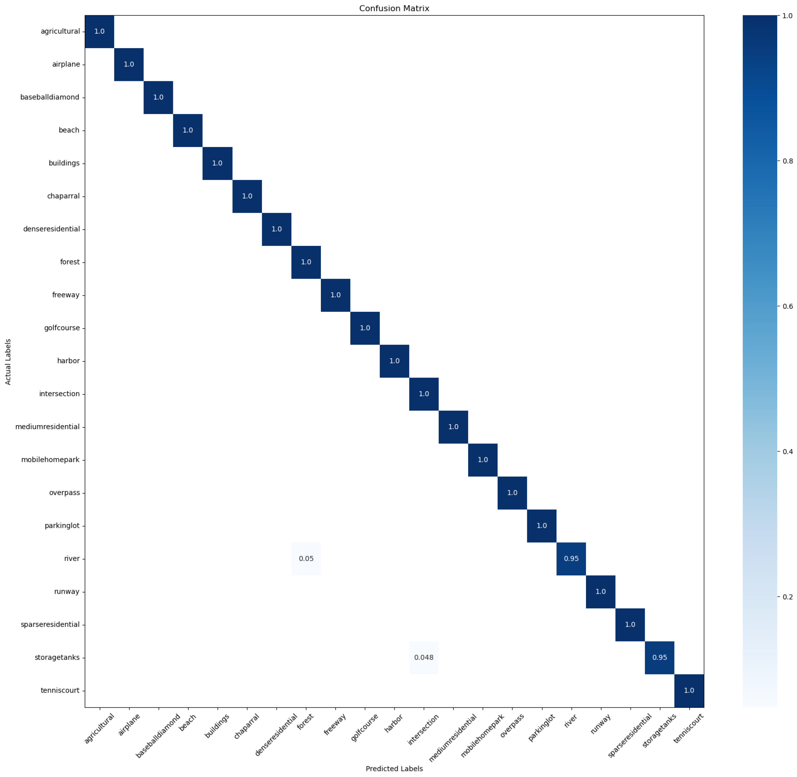
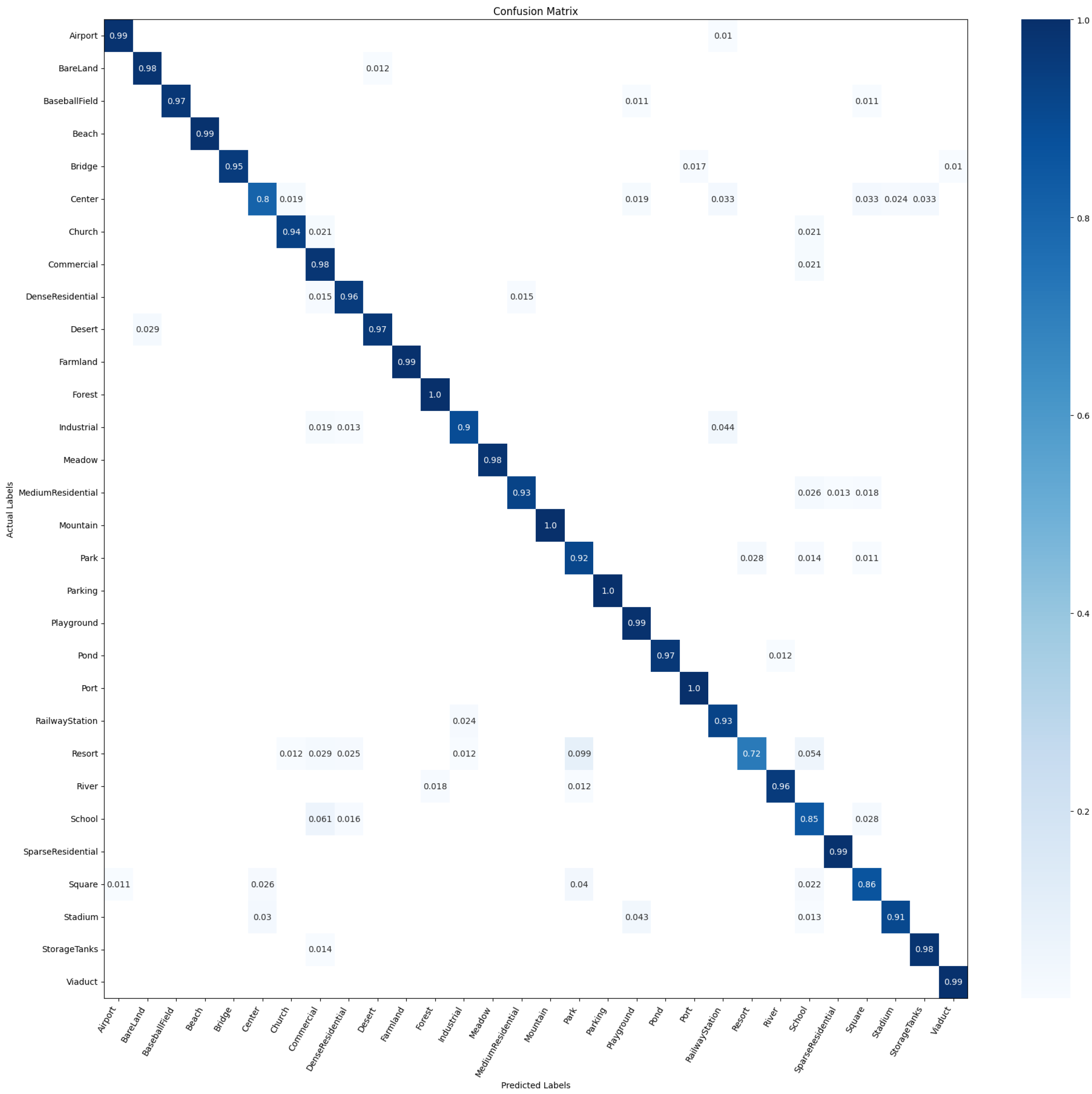
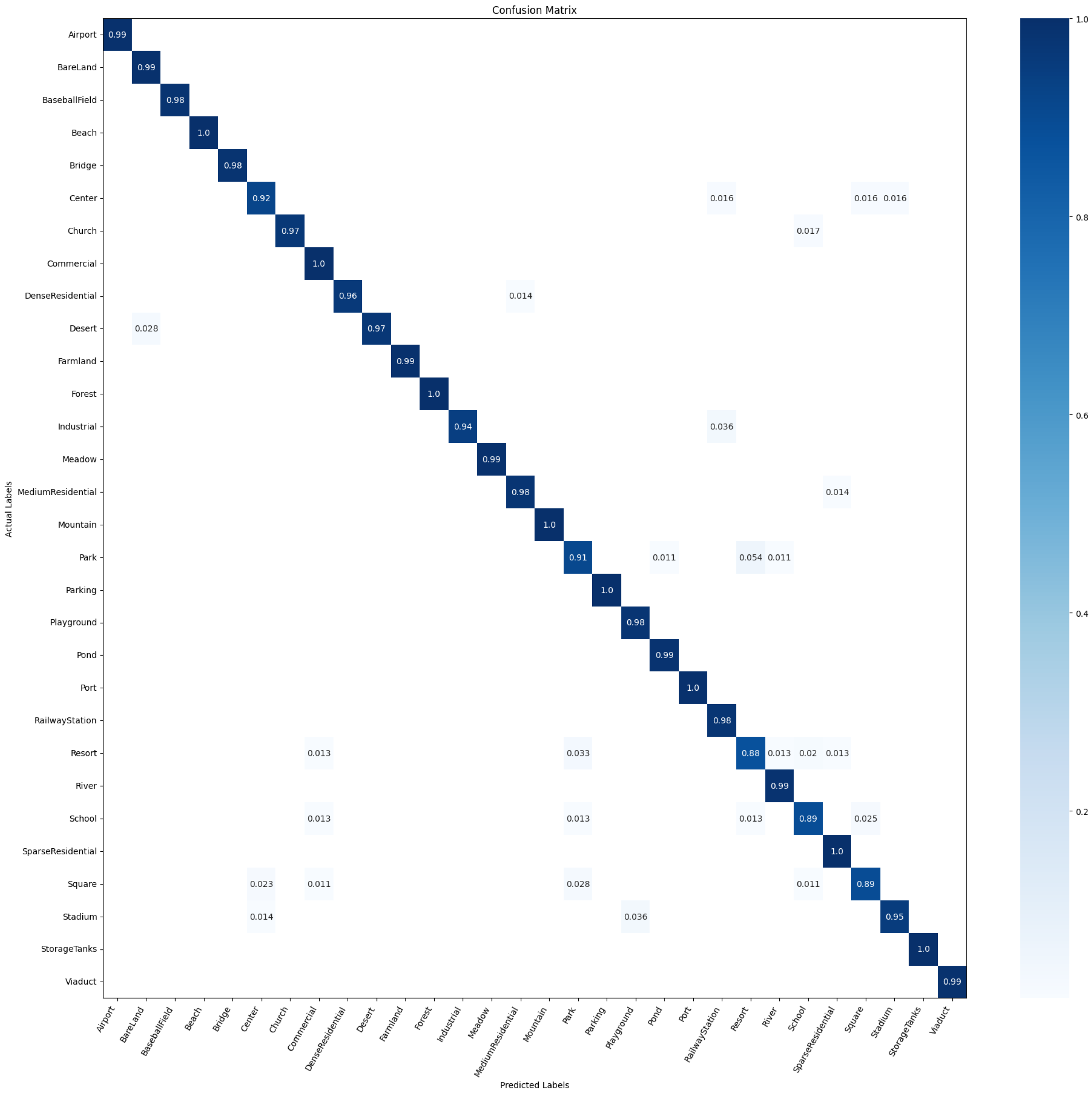
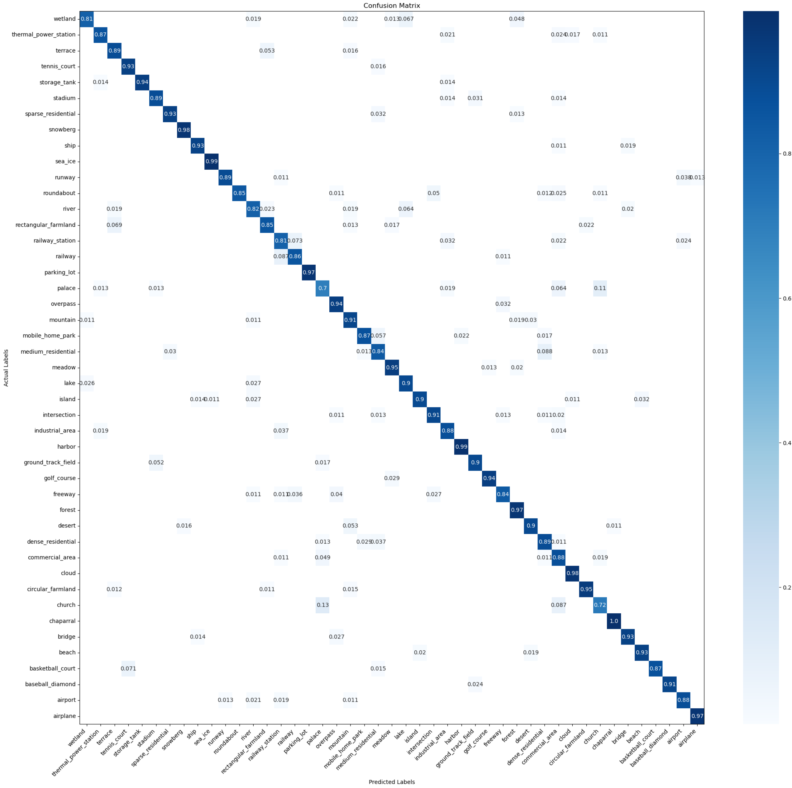
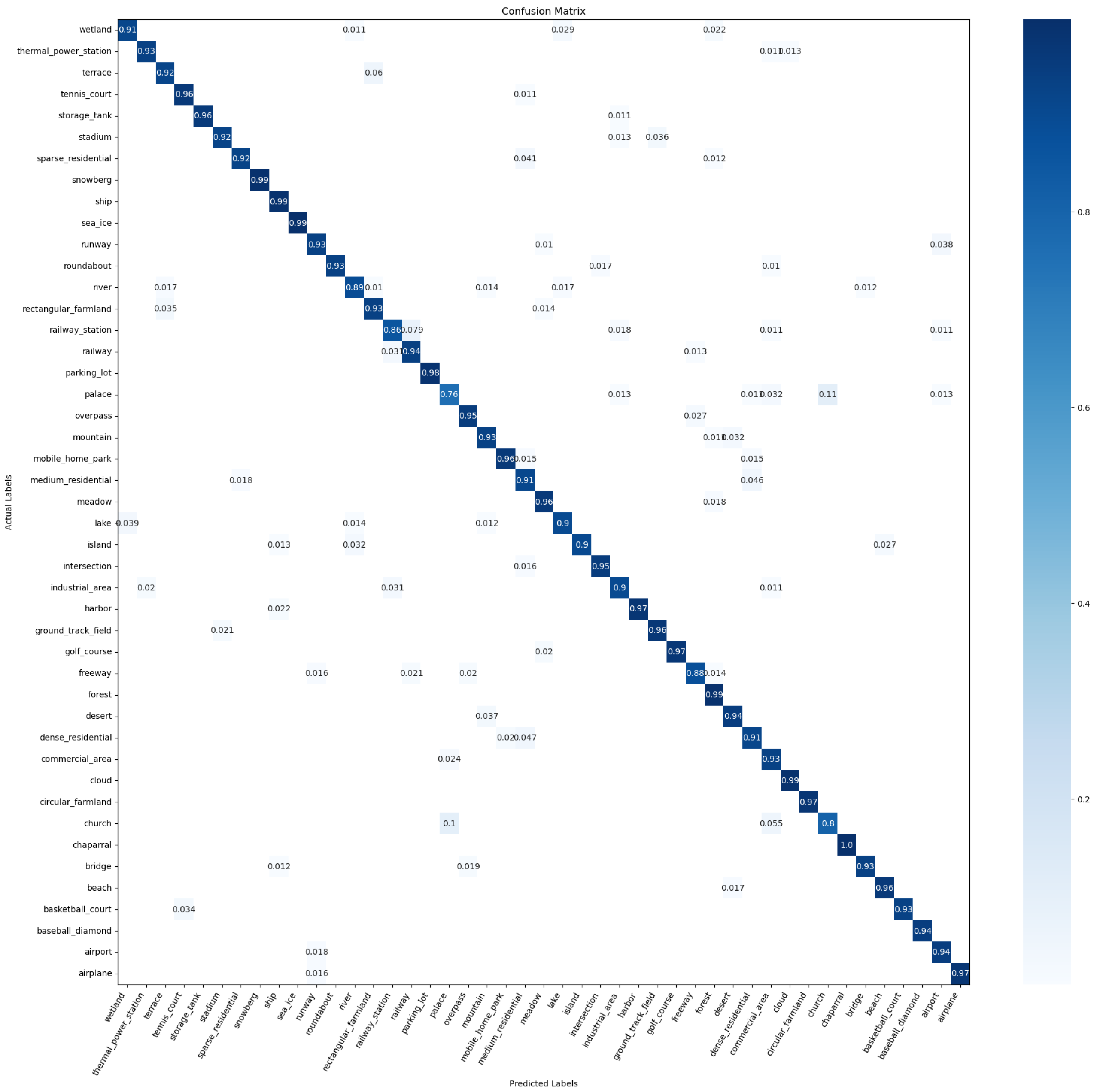
4.2.4. Confusion Matrix

The confusion matrix (CM) is an informative table designed to analyze errors and confusions among different categories. It is generated by tallying the correct and incorrect classifications for each type of test image and organizing these results within a table. The CM provides a detailed overview of classification outcomes, emphasizing misclassifications and serving as a complementary evaluation metric for overall accuracy. By highlighting specific areas where the model struggles, the confusion matrix aids in identifying potential improvements in classification performance.

4.3. Experiment Settings

4.3.1. Dataset Settings

Various data augmentation techniques were applied during the training of the base classifiers. These techniques included image flipping, image padding, image scaling, and image normalization. Image flipping involves horizontally or vertically flipping the input images, while image padding involves adding extra pixels around the borders of the images. Image scaling is used to resize the images to different resolutions, and image normalization aims to standardize the pixel values across the dataset. These data augmentation techniques help to increase the diversity of the training data and improve the robustness of the base classifiers. To ensure fairness and consistency in our experiments, the dataset partitioning method and random seed used in this study followed the same strategy as that employed by most remote sensing scene classification methods, such as T-CNN [10], PSGAN [43], and CSDS [44]. Specifically, the training and testing split for the UCM dataset was set at 80%:20%; for the AID dataset, the splits were 20%:80% and 50%:50%; and for the NWPU-RESISC45 dataset, the splits were 10%:90% and 20%:80%.

4.3.2. Structural Parameter Settings

In the stacking module, the selected base classifiers are convolutional neural networks with varying structures, ranging from a single convolutional layer to a maximum of 13 convolutional layers, augmented with an additional 3 layers of fully connected networks. This choice was made to leverage the capabilities of convolutional neural networks in capturing spatial features and extracting discriminative representations from the input data. In order to improve the overall performance of the RS scene classification task, we used the convolutional layer of the VGG16 model pretrained on the ImageNet dataset to initialize the convolutional layer in each base classifier during the stacking process.
To mitigate the effects of overfitting and ensure the generalization ability of the ensemble classifier, a 5-fold cross-validation strategy was employed during the training of the base classifiers. This approach involved partitioning the training data into 5 subsets, where each subset was separately used as a validation set, while the remaining data were used for training the base classifiers. By iteratively training the base classifiers on different validation sets, a more reliable estimate of their performance could be obtained. The outputs from the base classifiers were filtered using feature selection approaches. In this study, both wrapper and embedded feature selection methods were employed. The wrapper approach utilized a greedy strategy to eliminate underperforming base classifier results, while the embedded method incorporated 1 and 2 norms in the loss function of the meta-classifier. The hyperparameter ρ , which governs the magnitude of these two norms, was set to 0.01 in this study. By sparsifying the output of the meta-classifier, it identified a subset of base classifier results with the strongest predictive capabilities, thus enhancing the performance of the ensemble classifier.

4.3.3. Training Settings

In the autoencoder and the base classifier, the stochastic gradient descent and the Nesterov momentum with a momentum weight of 0.9 were used to train all the models. The number of training epochs was 500, and the batch size was 32. We used a weight decay of 10 4 and an initial learning rate of 0.01, and we decayed the learning rate with a cosine annealing. All experiments were carried out on a PC with an RTX-3090 GPU. The PyTorch (version 1.12.1), open-source framework and Python (version 3.7) programming language were used to implement the experiments. To mitigate the impact of random fluctuations, the experiment was repeated five times for each training ratio to obtain a more reliable assessment of the accuracies. This repeated experimentation allowed for the calculation of the average accuracies and standard deviations, providing a more comprehensive understanding of the classifier’s performance across different training ratios.

4.4. Results and Analysis

This section presents a detailed description and discussion of the experimental results obtained from the RS scene datasets. The objective was to validate the effectiveness of the proposed method by comparing it with state-of-the-art approaches from recent years. The results are reported in Table 2, Table 3 and Table 4.
On the UCM dataset [42], Table 2 presents the classification results of the proposed method and other state-of-the-art approaches. By analyzing the classification accuracy of each method in the table, it can be observed that handcrafted feature-based methods tend to suffer from limitations in feature extraction, which in turn affects the overall classification accuracy of the model. Conversely, most deep-feature-based methods achieve a classification accuracy above 90% and demonstrate stability. Notably, the proposed approach, LASMME, achieves a significantly higher classification accuracy of 99% than the other methods. Compared to recent deep learning models such as MGCAP [45], SEMSDNet [46], T-CNN [10], and DFAGCN [9], our method shows an overall accuracy improvement of 0.47%, 0.06%, 0.14%, and 0.99% respectively. This outcome further confirms that incorporating the latent associations between class distributions and imposing different penalties in cases of misclassification among different classes can effectively enhance classification accuracy.
On the AID dataset [12], Table 3 presents the classification performance of LSAMME and the other methods on the AID dataset [12]. The table includes two columns of results, representing the use of 20% and 50% of the samples for training, with the remaining samples allocated as the test set. By comparing the deep-feature-based methods, handcrafted feature-based methods, and the other methods, it is evident that the proposed method exhibits an improvement of at least 1% to 7% in classification accuracy when utilizing 20% and 50% of the samples for training. This substantial improvement highlights the advantage of integrating deep-learning-based classifiers. Furthermore, as the number of training samples increases, the gap in classification accuracy becomes more pronounced, indicating the demand for a sufficient number of training samples of CNNs-based methods. Notably, the proposed LSAMME achieves the highest classification performance of 94.92% and 97.16%.
Table 2. Comparison of OA and standard deviations (%) of state-of-the-art methods on the UCM dataset with a training ratio of 80%.
TypeMethodPublication Year(OA) Training Ratio 80%
(20% Testing)
BOVW(LBP) [12]TGRS201777.12 ± 1.93
BOVW(SIFT) [12]TGRS201774.12 ± 3.30
salM 3 LBP-CLM [47]JSTARS201795.75 ± 0.80
salCLM(eSIFT) [47]JSTARS201794.52 ± 0.79
Two-Fusion [1]CIN201898.02 ± 1.03
CCPNet [2]RS201897.52 ± 0.97
GCFs+LOFs [3]RS201899.00 ± 0.35
CNN-CapsNet [4]RS201999.05 ± 0.24
sCCov [5]TNNLS201999.05 ± 0.25
ARCNet-VGG [6]TGRS201999.12 ± 0.40
GBNet [48]TGRS202098.57 ± 0.48
MGCAP [45]TIP202099.00 ± 0.10
BiMobileNet [49]Sensors202099.03 ± 0.28
SEMSDNet [46]JSTARS202199.41 ± 0.41
T-CNN [10]TGRS202299.33 ± 0.11
DFAGCN [9]TNNLS202298.48 ± 0.42
OA: 99.47 ± 0.11
oursStacking-LSAMME AA: 99.47 ± 0.11
KC: 99.40 ± 0.12
†: handcrafted feature-based methods; ‡: deep methods. Bold indicates the best result. Italic indicates the second-best result.
Table 3. Comparison of OA and standard deviations (%) of state-of-the-art methods on the AID dataset with training ratios of 20% and 50%.
TypeMethod  Publication Year  (OA) Training Ratio
20% (80% Testing) 50% (50% Testing) 
BOVW(LBP) [12]TGRS201756.73 ± 0.5464.25 ± 0.55
BOVW(SIFT) [12]TGRS201761.40 ± 0.4167.65 ± 0.49
salM 3 LBP-CLM [47]JSTARS201786.92 ± 0.3589.76 ± 0.45
salCLM(eSIFT) [47]JSTARS201785.58 ± 0.8388.41 ± 0.63
VGG-VD-16 [12]RPOC201786.59 ± 0.2989.64 ± 0.36
Two-Fusion [1]CIN201892.32 ± 0.4194.58 ± 0.25
GCFs+LoFs [3]RS201892.48 ± 0.3896.85 ± 0.23
CNN-CapsNet [4]RS201993.79 ± 0.1396.32 ± 0.12
SCCov [5]TNNLS201993.12 ± 0.2596.10 ± 0.16
ARCNet-VGG [6]TGRS201988.75 ± 0.4093.10 ± 0.55
GBNet [48]TGRS202092.20 ± 0.2395.48 ± 0.12
MG-CAP [45]TIP201993.34 ± 0.1896.12 ± 0.12
CSDS [44]JSTARS202194.29 ± 0.3596.70 ± 0.14
PSGAN [43]TGRS202289.47± 0.3492.67 ± 0.55
T-CNN [10]TGRS202294.55 ± 0.2796.27 ± 0.23
OA: 94.92 ± 0.27OA: 97.16 ± 0.17
oursStacking-LSAMME AA: 94.62 ± 0.31AA: 97.05 ± 0.20
KC: 94.74 ± 0.34KC: 97.06 ± 0.23
†: handcrafted feature-based methods; ‡: deep methods. Bold indicates the best result. Italic indicates the second-best result.
On the NWPU-RESISC45 dataset [24], Table 4 presents a comparison of the results of the proposed method and the existing methods. When utilizing 10% and 20% of the samples as the training set, with the remaining samples allocated for testing, the proposed method exhibits superior performance to the other methods. By comparing deep-feature-based methods, handcrafted feature-based methods, and and the other methods, it is evident that the proposed method exhibits an improvement of at least 0.25% to 10% in classification accuracy when utilizing 10% and 20% of the sample for training. Furthermore, by examining the confusion matrix presented in Section 4.6, it can be observed that our model significantly reduces the probability of misclassifying similar classes. The absence of significant misclassification probabilities further supports the effectiveness and superiority of our proposed method.
Table 4. Comparison of OA and standard deviations (%) of state-of-the-art methods on the NWPU-RESISC45 dataset with training ratios of 10% and 20%.
TypeMethodPublication Year(OA) Train Ratios
10% (90% Testing)20% (80% Testing)
BOVW [24]RPOC201741.72 ± 0.2144.79 ± 0.28
BOVW+SPM [24]RPOC201727.83 ± 0.6132.96 ± 0.47
LLC [24]RPOC201738.81 ± 0.2340.03 ± 0.34
Fine-tuned VGG-16 [24]RPOC201787.15 ± 0.4590.36 ± 0.18
Two-Fusion [1]CIN201880.22 ± 0.2283.16 ± 0.18
D-CNN [50]TGRS201889.22 ± 0.5091.89 ± 0.22
Inception-v3-CapsNet [4]RS201989.03 ± 0.2192.60 ± 0.11
CNN-CapsNet [4]RS201989.03 ± 0.2192.60 ± 0.11
SCCov [5]TNNLS201989.30 ± 0.3592.10 ± 0.25
SF-CNN [51]TGRS201989.89 ± 0.1692.55 ± 0.14
RAN [52]TGRS201988.79 ± 0.5391.40 ± 0.30
GLANet [37]Access201989.50 ± 0.2691.50 ± 0.17
PSGAN [43]TGRS202284.72 ± 0.7288.47 ± 0.56
T-CNN [10]TGRS202290.25 ± 0.1193.05 ± 0.12
OA: 90.45 ± 0.15OA: 93.47 ± 0.12
oursStacking-LSAMME AA: 90.45 ± 0.15AA: 93.47 ± 0.12
KC: 90.11 ± 0.16KC: 93.26 ± 0.14
†: handcrafted feature-based methods; ‡: deep methods. Bold indicates the best result. Italic indicates the second-best result.

4.5. Ablation Experiment

In order to evaluate the impact of the category integration and feature selection modules on the performance of our proposed model (LSAMME), a series of ablative experiments were conducted. These experiments aimed to systematically analyze and assess the contribution of each module in enhancing the overall performance. Additionally, we validated the advantages of LSAMME compared to other classical algorithms when replacing the meta-learner in the stacking structure with them.
To ensure a rigorous experimental setup, we employed overall accuracy as the evaluation metric. As shown in Table 5, the experimental results in the last four rows of the table validate the effectiveness of the feature selection and category extraction modules. It is worth noting that the data in the third row were obtained with models lacking the category extraction module, which can be compared to the fifth row. Overall, the incorporation of both the category extraction and feature selection modules yields the best overall accuracy in the final results. The category distribution information extraction module facilitates the utilization of category-specific knowledge, enabling the model to capture nuanced patterns and make more accurate predictions, as shown in the fifth and sixth rows in Table 5. This result demonstrates the positive contribution of category information features to the experimental outcomes. From another perspective, the adjustment of sample weights in LSAMME leads to a more natural weighting of the samples, resulting in a training of base classifiers that is more reasonable. This helps to avoid the inclusion of weaker base classifiers in the meta layers of the ensemble. By appropriately adjusting the sample weights, LSAMME promotes the training of base classifiers that contribute more effectively to the ensemble’s overall performance. This result demonstrates the positive contribution of the image sample features extracted by effective base learners to the experimental outcomes. And, the feature selection module effectively identifies and utilizes the base layer’s classifier results, enhancing the model’s discrimination power. In Table 5, the first and second rows demonstrate that LSAMME as the meta layer in the stacking structure outperforms classical algorithms such as SVM [53] and GBDT [19].

4.6. Confusion Matrix

To enable an analysis of the classification results, a confusion matrix (CM) is utilized. The experimental results obtained using different training ratios on the UCM, AID, and NWPU-RESISC45 datasets yielded a total of five confusion matrices, which are depicted in Figure 6, Figure 7, Figure 8, Figure 9 and Figure 10.
Figure 6 illustrates the confusion matrix obtained from the testing set when the training set accounted for 80% on the UCM dataset. Among the 21 scene classes, only 2 classes, river and storagetanks, exhibit accuracies below 100%, achieving 95% accuracy. However, LSAMME still demonstrates unique advantages. For instance, it effectively captures the distinctions in information between mediumresidential and denseresidential, enabling the accurate differentiation between these two classes.
Figure 7 and Figure 8 display the confusion matrices obtained from the AID dataset when the training set accounts for 20% and 50%, respectively. When the training set comprised 20% of the samples, the accuracy of only three scene classes fell below 90%. The presence of numerous similar samples between the “resort” class and other classes, coupled with the limited number of training samples available, led to the decrease in accuracy. Consequently, the experimental performance on this particular class is relatively normal. However, the remaining classes exhibited excellent performance. Likewise, when the training set accounted for 50%, the accuracy of only two scene class fell below 90%. Notably, the accuracy oonf the “resort” class noticeably improves as the number of training samples increased.
Figure 9 and Figure 10 present the CM of the testing set obtained on the NWPU-RESISC45 dataset. When the proportion of training samples was 10% and 20%, the classification accuracy was above 90% for the majority of the scene classes. In the state-of-the-art (SOAT) method T-CNN [10], Palace was misclassified as a Church with a probability of 24%. However, our model demonstrates a significantly lower misclassification probability of only 10% for classifying Palace as Church.

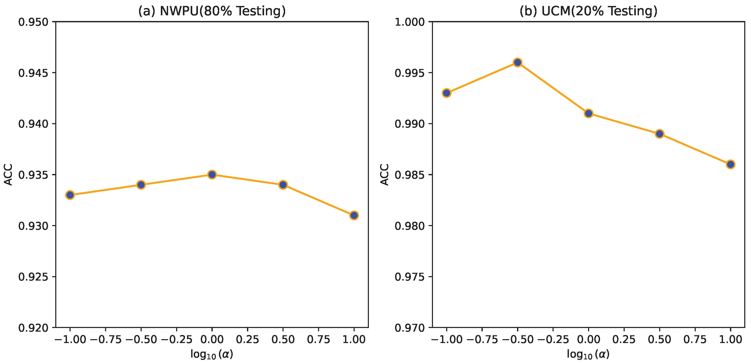
4.7. Parameter Sensitivity Experiment

In this study, we employed parameter α , as defined in Equation (6), to regulate the influence of category information on the classification process. The primary focus of this experiment was to investigate the sensitivity of the α parameter. It can be observed that when α = 0 , it is equivalent to the absence of category-guided information; SAMME was a specific case in this study. As the value of α increases, the degree of category guidance in the model progressively rises. The test accuracy, depicted in Figure 11, under various values of α on two datasets reveals a pattern where the model’s generalization performance initially improves and then deteriorates with the increase in α . This phenomenon aligns with our expectation, as α serves as a balancing factor. When α reaches a certain threshold, the model tends to focus more on challenging instances, neglecting the rest and causing a decline in overall performance.

5. Discussion

In this paper, we introduced a novel deep ensemble learning model that integrates category information with an ensemble learning framework, culminating in a new multiclass AdaBoost algorithm. This approach enables the model to focus more effectively on samples that are challenging to classify, particularly those situated near the decision boundary. Through theoretical analysis and empirical evaluations, we demonstrated the effectiveness and superiority of our proposed model compared to state-of-the-art methods. Our experiments, including ablation studies and confusion matrix analyses, showed that our model has significantly higher accuracy in classifying difficult-to-classify samples. However, sensitivity analysis revealed that an excessive emphasis on these challenging samples can lead to a decline in the accuracy of more easily separable samples. This highlights the need for a carefully calibrated balance parameter when integrating category information into the model.
The principles underlying our approach have broad applicability within the remote sensing domain, extending beyond scene classification to areas such as hyperspectral image classification and other related fields. Our findings confirm that incorporating prior information about category distributions and employing an ensemble learning framework can enhance model performance. Nevertheless, our methodology has certain limitations. In fitting the category distributions, we assumed that scene image samples conformed to a Gaussian distribution. Specifically, we acknowledge that, in some scene categories, the instance distribution exhibited complex and nonlinear characteristics, which could limit the applicability of the Gaussian assumption. Future work will explore the introduction of diverse sample distributions or adaptive sampling techniques to address this aspect. Additionally, while we utilized an autoencoder to extract category information from scene samples, we plan to investigate more advanced methods for this extraction in subsequent research.
Overall, our study provides a foundation for further exploration of the category distribution dynamics in remote sensing applications, and we are optimistic about the potential advancements that can be made by addressing the limitations outlined in this discussion.

6. Conclusions

In this paper, we proposed a remote sensing scene classification model based on the stacking ensemble approach, consisting of two main modules: an ensemble classification module and a category information extraction module. We elucidated the limitations of the relevant methods, which motivated our study, and provided detailed derivation of our approach. The theoretical analysis confirmed that the existing methods can be regarded as special cases of our approach. Furthermore, more weight is given to difficult samples that are difficult to classify in our method; the principle can be broadly applied to other classification models. In comparative experiments, our proposed method demonstrated improved performance in visual classification tasks compared to other neural network approaches.

Author Contributions

Conceptualization, Z.H., H.Y. and R.W.; Methodology, Z.H., H.Y. and R.W.; Software, G.L., H.Y. and R.W.; Validation, Z.W.; Formal analysis, Z.W. and G.H.; Investigation, Z.W.; Data curation, G.L.; Writing—original draft, G.L. and G.H. All authors have read and agreed to the published version of the manuscript.

Funding

This research was funded by the National Natural Science Foundation of China under Grant 62406250 and the Fundamental Research Funds for the Central Universities, in part by the Key Laboratory of Intelligent Equipment Application, Ministry of Education, Rocket Force University of Engineering, and the Natural Science Basic Research Plan in Shaanxi Province of China under Grant 2023-JC-QN-0702.

Data Availability Statement

Data are contained within the article.

Conflicts of Interest

The authors declare no conflicts of interest. The funders had no role in the design of the study; in the collection, analyses, or interpretation of data; in the writing of the manuscript; or in the decision to publish the results.

References

  1. Yu, Y.; Liu, F. A Two-Stream Deep Fusion Framework for High-Resolution Aerial Scene Classification. Comput. Intell. Neurosci. 2018, 18, 13. [Google Scholar] [CrossRef] [PubMed]
  2. Qi, K.; Guan, Q.; Yang, C.; Peng, F.; Shen, S.; Wu, H. Concentric Circle Pooling in Deep Convolutional Networks for Remote Sensing Scene Classification. Remote Sens. 2018, 10, 934. [Google Scholar] [CrossRef]
  3. Zeng, D.; Chen, S.; Chen, B.; Li, S. Improving Remote Sensing Scene Classification by Integrating Global-Context and Local-Object Features. Remote Sens. 2018, 10, 734. [Google Scholar] [CrossRef]
  4. Zhang, W.; Tang, P.; Zhao, L. Remote Sensing Image Scene Classification Using CNN-CapsNet. Remote Sens. 2019, 11, 494. [Google Scholar] [CrossRef]
  5. He, N.; Fang, L.; Li, S.; Plaza, J.; Plaza, A. Skip-Connected Covariance Network for Remote Sensing Scene Classification. IEEE Trans. Neural Networks Learn. Syst. 2020, 31, 1461–1474. [Google Scholar] [CrossRef]
  6. Wang, Q.; Liu, S.; Chanussot, J.; Li, X. Scene Classification With Recurrent Attention of VHR Remote Sensing Images. IEEE Trans. Geosci. Remote Sens. 2019, 57, 1155–1167. [Google Scholar] [CrossRef]
  7. Hao, Z.; Lu, Z.; Li, G.; Nie, F.; Wang, R.; Li, X. Ensemble clustering with attentional representation. IEEE Trans. Knowl. Data Eng. 2024, 36, 581–593. [Google Scholar] [CrossRef]
  8. Hao, Z.; Lu, Z.; Nie, F.; Wang, R.; Li, X. Multi-view k-means with laplacian embedding. In Proceedings of the ICASSP 2023—2023 IEEE International Conference on Acoustics, Speech and Signal Processing (ICASSP), Rhodes Island, Greece, 4–10 June 2023; IEEE: Piscataway, NJ, USA, 2023; pp. 1–5. [Google Scholar]
  9. Xu, K.; Huang, H.; Deng, P.; Li, Y. Deep Feature Aggregation Framework Driven by Graph Convolutional Network for Scene Classification in Remote Sensing. IEEE Trans. Neural Netw. Learn. Syst. 2022, 33, 5751–5765. [Google Scholar] [CrossRef]
  10. Wang, W.; Chen, Y.; Ghamisi, P. Transferring CNN With Adaptive Learning for Remote Sensing Scene Classification. IEEE Trans. Geosci. Remote Sens. 2022, 60, 1–18. [Google Scholar] [CrossRef]
  11. Wang, J.; Li, W.; Zhang, M.; Tao, R.; Chanussot, J. Remote sensing scene classification via multi-stage self-guided separation network. IEEE Trans. Geosci. Remote. Sens. 2023, 61, 1–12. [Google Scholar] [CrossRef]
  12. Xia, G.S.; Hu, J.; Hu, F.; Shi, B.; Bai, X.; Zhong, Y.; Zhang, L.; Lu, X. AID: A Benchmark Data Set for Performance Evaluation of Aerial Scene Classification. IEEE Trans. Geosci. Remote Sens. 2017, 55, 3965–3981. [Google Scholar] [CrossRef]
  13. Hao, Z.; Xin, H.; Wei, L.; Tang, L.; Wang, R.; Nie, F. Towards Expansive and Adaptive Hard Negative Mining: Graph Contrastive Learning via Subspace Preserving. In Proceedings of the ACM on Web Conference 2024, Singapore, 13–17 May 2024; pp. 322–333. [Google Scholar]
  14. Dong, X.; Yu, Z.; Cao, W.; Shi, Y.; Ma, Q. A survey on ensemble learning. Front. Comput. Sci. 2018, 14, 241–258. [Google Scholar] [CrossRef]
  15. Sun, G.; Cholakkal, H.; Khan, S.; Khan, F.; Shao, L. Fine-grained recognition: Accounting for subtle differences between similar classes. In Proceedings of the AAAI Conference on Artificial Intelligence, Vancouver, BC, Canada, 20–27 February 2020; Volume 34, pp. 12047–12054. [Google Scholar]
  16. Nie, F.; Hao, Z.; Wang, R. Multi-class support vector machine with maximizing minimum margin. In Proceedings of the AAAI Conference on Artificial Intelligence, Vancouver, BC, Canada, 20–28 February 2024; Volume 38, pp. 14466–14473. [Google Scholar]
  17. Sagi, O.; Rokach, L. Ensemble learning: A survey. Wiley Interdiscip. Rev. Data Min. Knowl. Discov. 2018, 8, 12–49. [Google Scholar] [CrossRef]
  18. Ma, L.; Sheng, Z.; Li, X.; Gao, X.; Hao, Z.; Yang, L.; Zhang, W.; Cui, B. Acceleration algorithms in gnns: A survey. arXiv 2024, arXiv:2405.04114. [Google Scholar]
  19. Freund, Y.; Schapire, R.; Abe, N. A short introduction to boosting. J.-Jpn. Soc. Artif. Intell. 1999, 14, 1612. [Google Scholar]
  20. Cao, D.; Xing, H.; Wong, M.S.; Kwan, M.P.; Xing, H.; Meng, Y. A Stacking Ensemble Deep Learning Model for Building Extraction from Remote Sensing Images. Remote Sens. 2021, 13, 3898. [Google Scholar] [CrossRef]
  21. Xin, H.; Hao, Z.; Sun, Z.; Wang, R.; Miao, Z.; Nie, F. Multi-view and Multi-order Graph Clustering via Constrained l1, 2-norm. Inf. Fusion 2024, 111, 102483. [Google Scholar] [CrossRef]
  22. Dong, Y.; Zhang, H.; Wang, C.; Zhou, X. Wind power forecasting based on stacking ensemble model, decomposition and intelligent optimization algorithm. Neurocomputing 2021, 462, 169–184. [Google Scholar] [CrossRef]
  23. Sun, R.; Wang, Y.; Zhang, Z.; Hong, R.; Wang, M. Deep adversarial inconsistent cognitive sampling for multiview progressive subspace clustering. IEEE Trans. Neural Netw. Learn. Syst. 2021. Available online: https://api.semanticscholar.org/CorpusID:231572752 (accessed on 26 October 2024). [CrossRef]
  24. Cheng, G.; Han, J.; Lu, X. Remote Sensing Image Scene Classification: Benchmark and State of the Art. Proc. IEEE 2017, 105, 1865–1883. [Google Scholar] [CrossRef]
  25. Wu, J.; Cui, Z.; Sheng, V.S.; Zhao, P.; Su, D.; Gong, S. A Comparative Study of SIFT and its Variants. Meas. Sci. Rev. 2013, 13, 122–131. [Google Scholar] [CrossRef]
  26. Pang, Y.; Yuan, Y.; Li, X.; Pan, J. Efficient HOG human detection. Signal Process. 2011, 91, 773–781. [Google Scholar] [CrossRef]
  27. LeCun, Y.; Boser, B.; Denker, J.S.; Henderson, D.; Howard, R.E.; Hubbard, W.; Jackel, L.D. Backpropagation Applied to Handwritten Zip Code Recognition. Neural Comput. 1989, 1, 541–551. [Google Scholar] [CrossRef]
  28. Simonyan, K.; Zisserman, A. Very Deep Convolutional Networks for Large-Scale Image Recognition. arXiv 2014, arXiv:1409.1556. [Google Scholar]
  29. Chatzimparmpas, A.; Martins, R.M.; Kucher, K.; Kerren, A. StackGenVis: Alignment of Data, Algorithms, and Models for Stacking Ensemble Learning Using Performance Metrics. IEEE Trans. Vis. Comput. Graph. 2021, 27, 1547–1557. [Google Scholar] [CrossRef]
  30. Freund, Y.; Schapire, R.E. A decision-theoretic generalization of on-line learning and an application to boosting. J. Comput. Syst. Sci. 1997, 55, 119–139. [Google Scholar] [CrossRef]
  31. Zhu, J.; Zou, H.; Rosset, S.; Hastie, T. Mult-class Adaboost. Stat. Its Interface 2009, 2, 349–360. [Google Scholar]
  32. Dai, X.; Wu, X.; Wang, B.; Zhang, L. Semisupervised scene classification for remote sensing images: A method based on convolutional neural networks and ensemble learning. IEEE Geosci. Remote Sens. Lett. 2019, 16, 869–873. [Google Scholar] [CrossRef]
  33. Zhao, Q.; Lyu, S.; Li, Y.; Ma, Y.; Chen, L. MGML: Multigranularity multilevel feature ensemble network for remote sensing scene classification. IEEE Trans. Neural Networks Learn. Syst. 2021, 34, 2308–2322. [Google Scholar] [CrossRef]
  34. Li, J.; Gong, M.; Liu, H.; Zhang, Y.; Zhang, M.; Wu, Y. Multiform ensemble self-supervised learning for few-shot remote sensing scene classification. IEEE Trans. Geosci. Remote Sens. 2023, 61, 1–16. [Google Scholar] [CrossRef]
  35. Hui, L.; Li, X.; Gong, C.; Fang, M.; Zhou, J.T.; Yang, J. Inter-class angular loss for convolutional neural networks. In Proceedings of the AAAI Conference on Artificial Intelligence, Honolulu, HI, USA, 27 January–1 February 2019; Volume 33, pp. 3894–3901. [Google Scholar]
  36. Feng, L.; Wang, H.; Jin, B.; Li, H.; Xue, M.; Wang, L. Learning a distance metric by balancing kl-divergence for imbalanced datasets. IEEE Trans. Syst. Man, Cybern. Syst. 2018, 49, 2384–2395. [Google Scholar] [CrossRef]
  37. Guo, Y.; Ji, J.; Lu, X.; Huo, H.; Fang, T.; Li, D. Global-Local Attention Network for Aerial Scene Classification. IEEE Access 2019, 7, 67200–67212. [Google Scholar] [CrossRef]
  38. Yarotsky, D. Error bounds for approximations with deep ReLU networks. Neural Netw. 2017, 94, 103–114. [Google Scholar] [CrossRef] [PubMed]
  39. Xia, Y.; Chen, K.; Yang, Y. Multi-label classification with weighted classifier selection and stacked ensemble. Inf. Sci. 2021, 557, 421–442. [Google Scholar] [CrossRef]
  40. Riccardi, A.; Fernández-Navarro, F.; Carloni, S. Cost-sensitive AdaBoost algorithm for ordinal regression based on extreme learning machine. IEEE Trans. Cybern. 2014, 44, 1898–1909. [Google Scholar] [CrossRef]
  41. Zou, H.; Hastie, T. Regularization and variable selection via the elastic net. J. R. Stat. Soc. Ser. B Stat. Methodol. 2005, 67, 301–320. [Google Scholar] [CrossRef]
  42. Yang, Y.; Newsam, S. Bag-of-visual-words and spatial extensions for land-use classification. In Proceedings of the 18th SIGSPATIAL International Conference on Advances in Geographic Information Systems, San Jose, CA, USA, 2–5 November 2010; pp. 270–279. [Google Scholar] [CrossRef]
  43. Cheng, G.; Sun, X.; Li, K.; Guo, L.; Han, J. Perturbation-Seeking Generative Adversarial Networks: A Defense Framework for Remote Sensing Image Scene Classification. IEEE Trans. Geosci. Remote Sens. 2022, 60, 1–11. [Google Scholar] [CrossRef]
  44. Wang, Y.; Xiao, R.; Qi, J.; Tao, C. Cross-Sensor remote sensing Images Scene Understanding Based on Transfer Learning Between Heterogeneous Networks. IEEE Geosci. Remote Sens. Lett. 2022, 19, 1–5. [Google Scholar] [CrossRef]
  45. Wang, S.; Guan, Y.; Shao, L. Multi-Granularity Canonical Appearance Pooling for Remote Sensing Scene Classification. IEEE Trans. Image Process. 2020, 29, 5396–5407. [Google Scholar] [CrossRef]
  46. Tian, T.; Li, L.; Chen, W.; Zhou, H. SEMSDNet: A Multiscale Dense Network With Attention for Remote Sensing Scene Classification. IEEE J. Sel. Top. Appl. Earth Obs. Remote Sens. 2021, 14, 5501–5514. [Google Scholar] [CrossRef]
  47. Bian, X.; Chen, C.; Tian, L.; Du, Q. Fusing Local and Global Features for High-Resolution Scene Classification. IEEE J. Sel. Top. Appl. Earth Obs. Remote Sens. 2017, 10, 2889–2901. [Google Scholar] [CrossRef]
  48. Sun, H.; Li, S.; Zheng, X.; Lu, X. Remote Sensing Scene Classification by Gated Bidirectional Network. IEEE Trans. Geosci. Remote Sens. 2020, 58, 82–96. [Google Scholar] [CrossRef]
  49. Yu, D.; Xu, Q.; Guo, H.; Zhao, C.; Lin, Y.; Li, D. An Efficient and Lightweight Convolutional Neural Network for Remote Sensing Image Scene Classification. Sensors 2020, 20, 1999. [Google Scholar] [CrossRef] [PubMed]
  50. Cheng, G.; Yang, C.; Yao, X.; Guo, L.; Han, J. When Deep Learning Meets Metric Learning: Remote Sensing Image Scene Classification via Learning Discriminative CNNs. IEEE Trans. Geosci. Remote Sens. 2018, 56, 2811–2821. [Google Scholar] [CrossRef]
  51. Xie, J.; He, N.; Fang, L.; Plaza, A. Scale-Free Convolutional Neural Network for Remote Sensing Scene Classification. IEEE Trans. Geosci. Remote Sens. 2019, 57, 6916–6928. [Google Scholar] [CrossRef]
  52. Fan, R.; Wang, L.; Feng, R.; Zhu, Y. Attention based Residual Network for High-Resolution Remote Sensing Imagery Scene Classification. In Proceedings of the IGARSS 2019—2019 IEEE International Geoscience and Remote Sensing Symposium, Yokohama, Japan, 28 July–2 August 2019; pp. 1346–1349. [Google Scholar] [CrossRef]
  53. Scholkopf, B. Making large scale SVM learning practical. In Advances in Kernel Methods: Support Vector Learning; MIT Press: Cambridge, MA, USA, 1999; pp. 41–56. [Google Scholar]
Figure 1. Schematic illustration of the proposed model. The model is primarily divided into two modules: category distribution information extraction and scene classification. In the category distribution information extraction module, there are three components: the autoencoder, Gaussian model fitting, and the computation of category similarity. We employ an autoencoder to extract scenes’ low-dimensional features. These extracted scene features are then used to fit the scene category distributions, and the similarities between the category distributions are computed. In the scene classification module, we employ a stacking ensemble approach, which consists of three parts: the base learners, feature selection, and LSAMME. The base layer consists of CNNs, and the meta layer utilizes a novel multiclass AdaBoost method that incorporates fused category distribution information.
Remotesensing 16 04084 g001
Figure 2. An illustrative plot for Lake, Church, and Palace highlights that, in comparison to the Lake–Church and Lake–Palace pairs, there exists a subset of highly similar samples between the categories of Church and Palace. This observation indicates that differentiating between the boundary samples of Church and Palace can be challenging.
Remotesensing 16 04084 g002
Figure 3. Several examples of scenes in the UCM dataset. The categories are (a) agricultural, (b) airplane, (c) buildings, (d) harbor, and (e) parkinglot.
Remotesensing 16 04084 g003
Figure 4. Several examples of scenes in the AID dataset. The categories are (a) Bridge, (b) Center, (c) Desert, (d) Industrial, and (e) Mountain.
Remotesensing 16 04084 g004
Figure 5. Several examples of scenes in the NWPU-RESISC45 dataset. The categories are (a) Airport, (b) Beach, (c) Forest, (d) Lake, and (e) Mountain.
Remotesensing 16 04084 g005
Figure 6. CM on the UCM dataset with 80% of the dataset used for training and the rest for testing.
Remotesensing 16 04084 g006
Figure 7. CM on the AID dataset with 20% of the dataset used for training and the rest for testing.
Remotesensing 16 04084 g007
Figure 8. CM on the AID dataset with 50% of the dataset used for training and the rest for testing.
Remotesensing 16 04084 g008
Figure 9. CM on the NWPU-RESISC45 dataset with 10% of the dataset used for training and the rest for testing.
Remotesensing 16 04084 g009
Figure 10. CM on the NWPU-RESISC45 dataset with 20% of the dataset used for training and the rest for testing.
Remotesensing 16 04084 g010
Figure 11. The effect of parameter α on the experimental results.
Remotesensing 16 04084 g011
Table 1. Description of datasets.
DatasetInstancesFeaturesClassesResolution
UCM dataset2100256 × 256210.3 m
AID dataset10,000600 × 600300.5–8 m
NWPU-RESISC45231,500256 × 256450.2–30 m
Table 5. Ablation study of the proposed method (LSAMME) on different datasets. We compare LSAMME and its variants by removing feature selection and category information. (The symbol ✓ indicates that the model includes the specified module during the experiment. And bold indicates the best result.)
Stacking CNNFeature SelectionSVMGBDTSAMMELSAMMENWPU (10%)NWPU (20%)UCM (80%)
88.34± 0.2692.98± 0.1997.76 ± 0.23
89.07± 0.2192.95± 0.2197.98 ± 0.18
88.67± 0.2192.65± 0.1698.21 ± 0.12
89.26± 0.1793.07± 0.1198.88 ± 0.14
89.67± 0.1493.30± 0.1299.21 ± 0.12
90.45 ± 0.1593.47± 0.1299.47 ± 0.11
Disclaimer/Publisher’s Note: The statements, opinions and data contained in all publications are solely those of the individual author(s) and contributor(s) and not of MDPI and/or the editor(s). MDPI and/or the editor(s) disclaim responsibility for any injury to people or property resulting from any ideas, methods, instructions or products referred to in the content.

