A Multi-Scale Feature Fusion Deep Learning Network for the Extraction of Cropland Based on Landsat Data

Abstract

In the face of global population growth and climate change, the protection and rational utilization of cropland are crucial for food security and ecological balance. However, the complex topography and unique ecological environment of the Qinghai-Tibet Plateau results in a lack of high-precision cropland monitoring data. Therefore, this paper constructs a high-quality cropland dataset for the YarlungZangbo-Lhasa-Nyangqv River region of the Qinghai-Tibet Plateau and proposes an MSC-ResUNet model for cropland extraction based on Landsat data. The dataset is annotated at the pixel level, comprising 61 Landsat 8 images in 2023. The MSC-ResUNet model innovatively combines multiscale features through residual connections and multiscale skip connections, effectively capturing features ranging from low-level spatial details to high-level semantic information and further enhances performance by incorporating depthwise separable convolutions as part of the feature fusion process. Experimental results indicate that MSC-ResUNet achieves superior accuracy compared to other models, with F1 scores of 0.826 and 0.856, and MCC values of 0.816 and 0.847, in regional robustness and temporal transferability tests, respectively. Performance analysis across different months and band combinations demonstrates that the model maintains high recognition accuracy during both growing and non-growing seasons, despite the study area’s complex landforms and diverse crops.

1. Introduction

In light of challenges like global population growth and climate change, the protection and rational utilization of cropland have become pivotal to food security and ecological balance [1]. Cropland serves as the foundation of agricultural production, maintains biodiversity, and fosters economic growth in local communities [2]. Changes in cropland area and quality reflect the interaction between natural conditions and human activities, making it a key research area in environmental science and geography [3,4].

With the advancement of remote sensing technology, extracting cropland information from satellite imagery has become increasingly common [5]. Traditional methods for cropland extraction fall into two categories: single-temporal image-based machine learning methods and multi-temporal data-based time series analysis methods [6]. Single-temporal image-based methods analyze features from images taken during a single time period, utilizing visible and near-infrared bands, spectral indices, texture features, and terrain information. Machine learning classifiers like random forests, support vector machines, or decision trees are commonly used to process these features and extract cropland data [7,8,9]. However, these methods are limited by single-period data constraints and cloud cover. Time series analysis involves extracting temporal features or phenological indices from a series of images taken over time. Techniques include using vegetation indices for rule-based classification and statistical methods to calculate metrics like maximum vegetation index and time to peak vegetation index [10,11,12,13]. More complex methods construct multi-source vegetation index time series or use advanced temporal feature extractors to enhance accuracy [14,15]. While these methods achieve high classification accuracy and capture crop growth cycles, they require extensive time-series data and expertise.

The rapid development of deep learning technology has led to significant progress in satellite imagery processing [16,17], with methods such as Convolutional Neural Networks (CNN) being applied to cropland extraction tasks [18,19]. Deep learning methods, by constructing multi-layer neural networks, can automatically learn and extract complex features from images, thereby achieving higher accuracy in cropland extraction.

Some deep learning models that integrate multi-temporal data, such as Recurrent Neural Networks (RNN) [20] and Long Short-Term Memory networks (LSTM) [21], have been applied to the extraction of cropland information. These methods can better capture vegetation changes by utilizing time series data [22,23]. However, these methods require high temporal continuity and consistency of data, which is often challenging due to cloud cover, rainfall, or inconsistent satellite pass times. Studies have shown that LSTM does not perform as well as traditional non-deep learning classifiers and one-dimensional convolutional neural networks when dealing with multi-temporal Landsat data for crop information extraction [24].

Single-temporal semantic segmentation models have shown significant results in cropland extraction. Encoder-decoder frameworks like SegNet [25] and U-Net [26] have been widely applied. For example, SegNet combined with Sentinel-2A satellite data achieved an average F1 score of 0.84 at classifying land use and land cover in Indian regions [27]. An attention-based U-Net model optimized with Focal Tversky Loss used Landsat 8 and Sentinel-2 data to map crop types in the U.S. Corn Belt [28]. Additionally, a ResUNet model combined with a long-term series cropland correction algorithm produced annual cropland maps for Guangdong Province from 1991 to 2020 using Landsat data [29].

Current remote sensing deep semantic segmentation models follow several key principles. They reduce feature map resolution through pooling, stride adjustments, or dilated convolutions to capture high-level semantic features and expand the receptive field for more complex representations. These low-resolution feature maps are then upsampled and combined with their downsampled counterparts to restore high-resolution features, enhancing segmentation performance. Low-level feature maps capture detailed spatial information and object boundaries, while high-level maps provide positional information to locate objects [30]. However, this downsampling and upsampling process can dilute the signal of object boundaries, especially with 30-m resolution Landsat data. Common downsampling practices reduce this resolution to 480 m, leading to coarse segmentation and loss of critical details if not properly managed [6]. Balancing low-level spatial features and high-level semantic features to maintain precision and detail is a significant challenge for deep learning models dealing with medium-resolution imagery [26,31,32].

Another major challenge in extracting cropland information using Landsat data in Qinghai-Tibet Plateau is the lack of high-quality training datasets. Deep learning models require a large, uniformly distributed dataset of training samples to prevent overfitting and improve generalization [33,34]. Compared to high-resolution data, pixel-level annotation of Landsat data is more time-consuming and difficult. Although the availability of open training datasets has significantly advanced deep learning technologies, the spatial consistency of currently shared medium-resolution datasets in the Qinghai-Tibet Plateau region is still far from ideal [35].

Facing the issues of lacking high-quality training datasets for Landsat imagery in the Qinghai-Tibet Plateau and the insufficient information flow utilization between low-level spatial features and high-level semantic features in existing deep learning models for Landsat data, this paper presents a high-quality training dataset with pixel-level accuracy based on Landsat data from the YarlungZangbo-Lhasa-Nyangqv River region of the Qinghai-Tibet Plateau. The primary objective of this study is to enhance the accuracy of cropland extraction from 30-m resolution Landsat multispectral data while also reducing computational costs. Subsequently, a novel MSC-ResUNet (Multi-Scale Skip Connections ResUNet) model is proposed, which combines multiscale features through residual connections and multiscale skip connections, while further enhancing performance by incorporating depthwise separable convolutions as part of the feature fusion process. This approach aims to enhance the accuracy of cropland extraction from 30-m resolution Landsat multispectral data by improving feature utilization and reducing computational costs. Leveraging these advancements, the proposed model seeks to deliver more precise and detailed segmentation results for fragmented cropland areas. The overall workflow was shown in Figure 1.

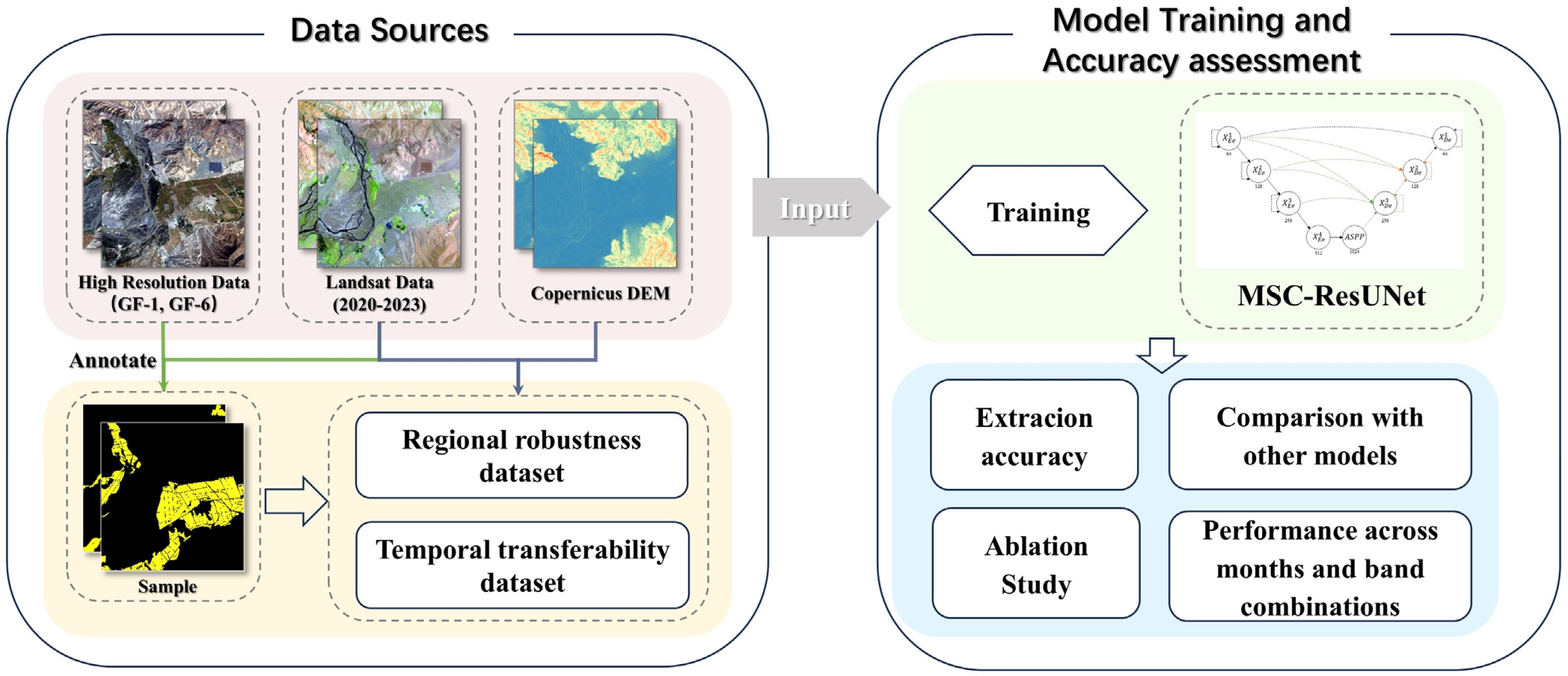
2. Materials and Methods

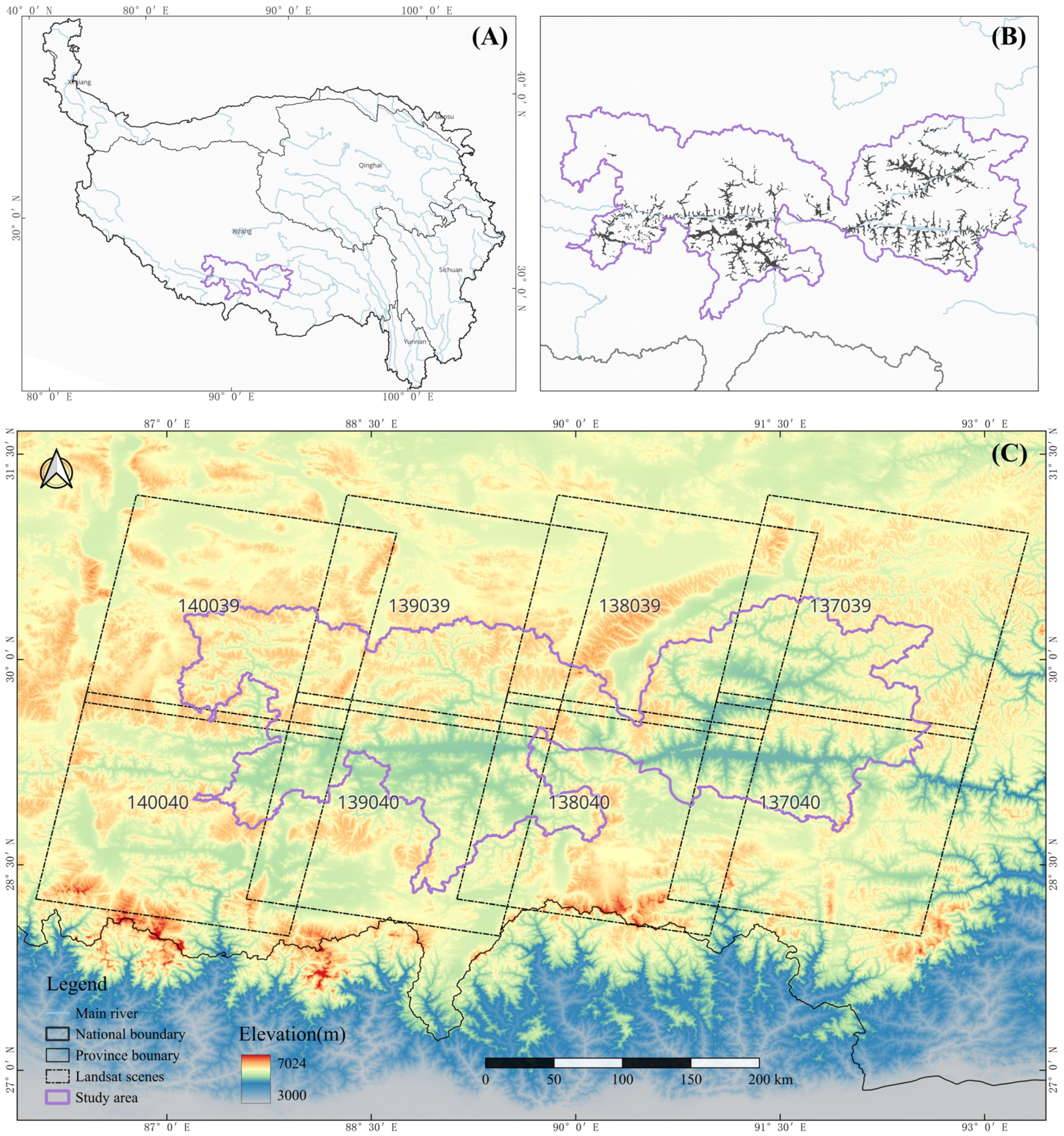
2.1. Study Area

The YarlungZangbo-Lhasa-Nyangqv River region (87°04′E–92°37′E, 28°17′N–30°28′N) lies in the central Qinghai-Tibet Plateau, encompassing the middle reaches of the Yarlung Zangbo River and its tributaries, the Lhasa and Nyangqv Rivers. This region, an important agricultural base and grain-producing area in the Xizang Autonomous Region, spans approximately 66,700 km², or 5.52% of the region’s total area, with altitudes ranging from 2700 to 4200 m [36].

The region features a plateau temperate monsoon semi-arid climate, with average annual temperatures between 4.7 and 8.3 °C and annual precipitation from 251.7 to 580.0 mm, mostly occurring from May to September [37]. Major crops include barley and wheat, with some areas growing winter wheat [38,39]. This region accounts for over 60% of Tibet’s total cropland [40]. The distribution of cropland in this area is markedly dispersed, primarily concentrated along river valleys and alluvial plains. This pattern is influenced by the region’s varied topography and geomorphology, resulting in irregular patches of cropland interspersed with non-crop areas [41,42]. The fragmented terrain, combined with the effects of slope and soil conditions [43], leads to cropland being scattered rather than consolidated into large, contiguous fields, as shown in Figure 2.

2.2. Dataset

2.2.1. Landsat Data

This paper used the Level 2, Collection 2, Tier 1 dataset from the Landsat 8 satellite provided by the USGS, covering the years 2020 to 2023. The Worldwide Reference System (WRS) paths and rows of the selected data are 137/039-040, 138/039-040, 139/039-040, and 140/039-040, as shown in Figure 2. To enhance data quality and minimize cloud interference, images with less than 30% cloud cover were filtered, and the quality assessment bands were used for cloud removal, forming the training and prediction datasets. Before model input, the images were normalized, as detailed in in Equation (1):

$$\rho =DN\times scale+offset$$

(1)

where ρ is the surface reflectance (normalization value) as the input of model, scale and offset are parameters from the metadata file with values of 0.0000275 and 0.2, and DN represents the digital number for each band.

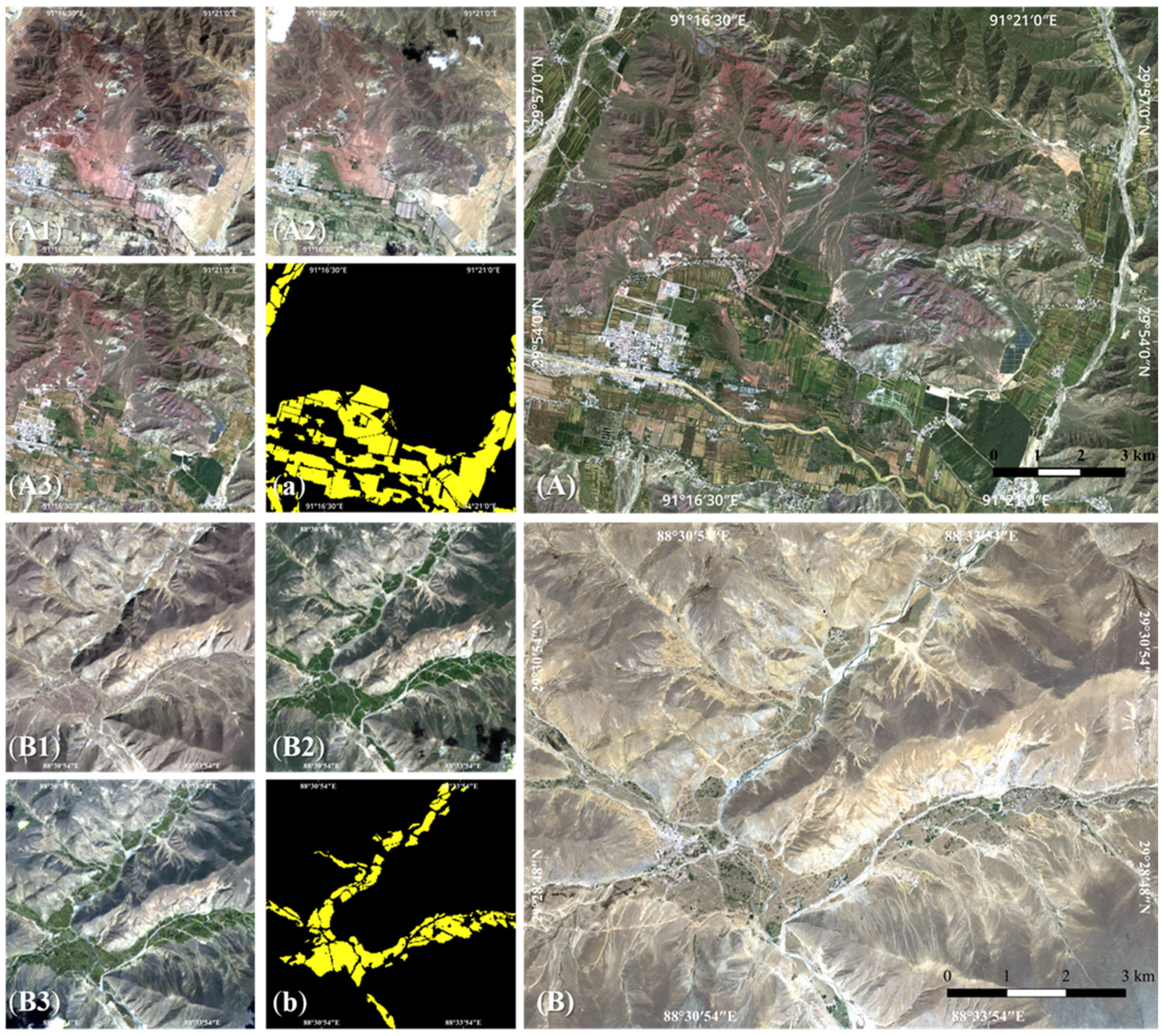
2.2.2. Annotation of Cropland

In this paper, cropland encompasses land used for growing crops, including cultivated land, newly developed or reclaimed land, managed land, and fallow land (including rotational fallow land and resting land). This definition primarily covers land for crops, sometimes interspersed with fruit trees, mulberry trees, or other trees. However, the definition excludes small plots of cropland less than 0.09 ha (minimum width of 30 m) and facility agriculture, such as greenhouses, due to their distinct spectral signatures in remote sensing images.

The accurate annotation of cropland in the study area using Landsat data is a challenging process, particularly given its fragmented and scattered distribution. To address this challenge, high-resolution images (The Gaofen-1 satellite and the Gaofen-6 satellite, with 2-m resolution) from the corresponding year’s growing season were employed as reference data. The annotation process entailed the manual identification of cropland plots, based on an examination of their characteristics in high-resolution images and an analysis of crop phenological features in multi-temporal Landsat images.

In two representative study areas, the spatial distribution of cropland is illustrated, highlighting its fragmented and scattered nature (Figure 3). Figure 3A,B show images from the Gaofen-1 satellite (2 September 2023) and the Gaofen-6 satellite (17 May 2020), respectively. During these periods, most crops were in the reproductive growth to maturity and harvest stages, exhibiting distinct spectral and textural information compared to surrounding land features, which facilitated accurate cropland annotation. Figure 3(A1–A3,B1–B3) display Landsat 8 images of regions Figure 3A,B from different months between March and September. These images demonstrate significant temporal variation in cropland spectral information.

To ensure the quality and reliability of the annotated samples, a validation dataset of 2508 sample points was constructed. The validation points were generated from cropland distributions from ESA [44], GLC-30 [45] and our own product within the study area. Specifically, we randomly generated validation points based on the combined spatial distributions of cropland and non-cropland from these three sources. Then, the classification of these points as cropland or non-cropland was determined through visual interpretation using domestically produced high-resolution images. As a result, the validation samples are unevenly distributed, clustering mostly near cropland (Figure 4). This focus aligns with the study’s primary objective extracting cropland rather than all land cover types, emphasizing the verification of extraction accuracy in these scenarios. The accuracy and confusion matrix of the sample dataset are presented in

Table 1. Confusion matrix of the sample dataset accuracy.

		Truth
		Cropland	Non-Cropland	Total	Precision
Prediction	Cropland	1289	20	1309	0.985
	Non-Cropland	34	1165	1199	0.972
	Total	1323	1185
	Recall	0.974	0.983
	MCC	0.9795
	Overall Accuracy	0.9784

, yielding an F1 score of 0.9795 and an overall accuracy of 0.9784.

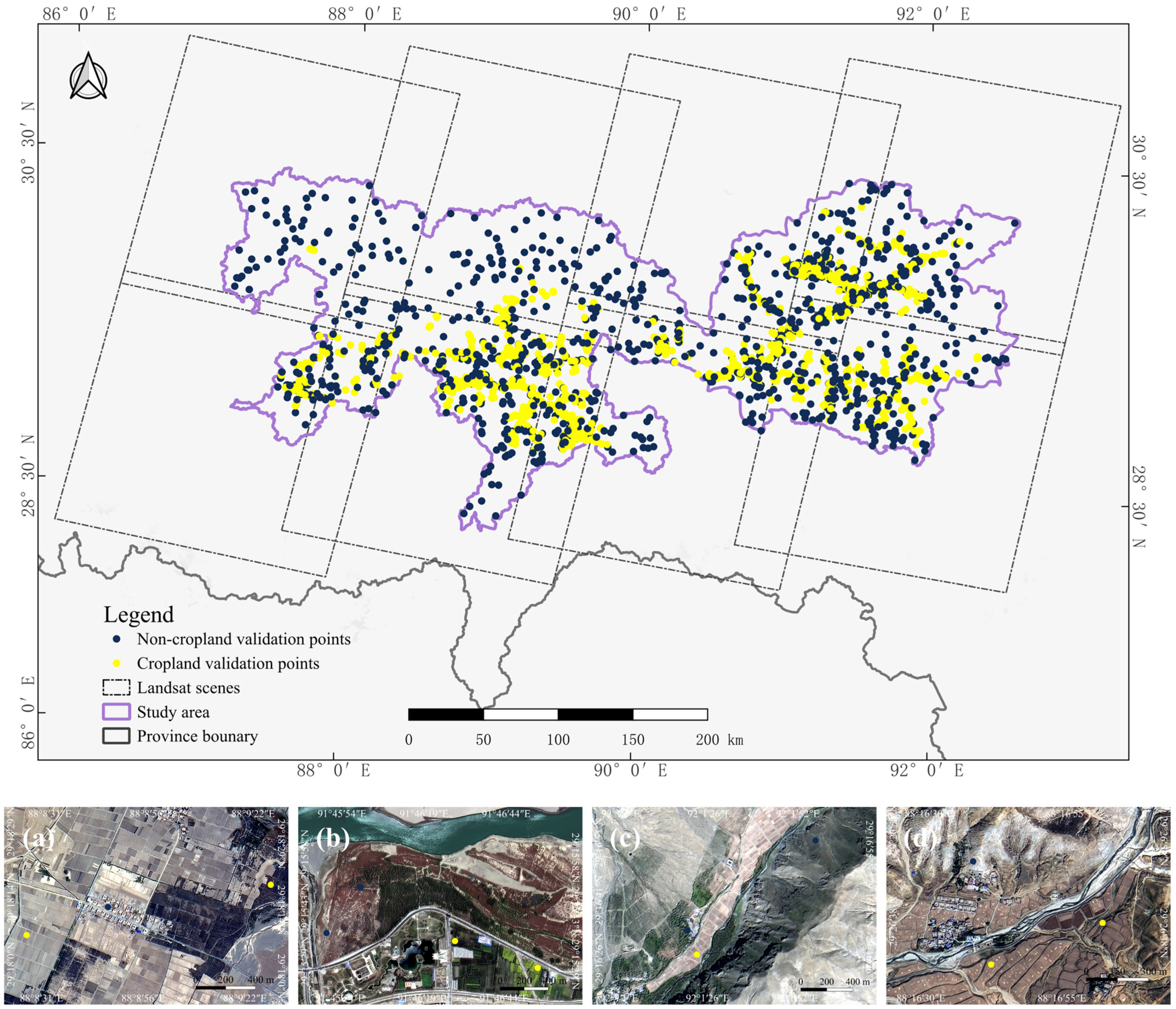
2.2.3. Construction of Dataset

To guarantee the impartiality of the model assessment, this study constructed two datasets: a regional robustness dataset and a temporal transferability dataset. These datasets test the model’s performance across different regions and time periods.

The regional robustness dataset includes 34 scenes of Landsat images from 2023, covering path and row numbers 137/039, 137/040, 138/040, 139/039, 139/040, and 140/039 as the training dataset, and 12 scenes of Landsat images with path and row numbers 138/039 and 140/040 as the validation dataset. To ensure the independence and reliability of the validation dataset, any overlap with training images was removed.

The temporal transferability dataset shares the same training dataset as the regional robustness dataset. The validation dataset, however, consists of 11 scenes of Landsat images from 2020 and 2021, taken during different months but from the same paths and rows. For instance, for the region 139/039, the training dataset includes images from 6 April, 8 May, 25 June, 13 September, 15 October, and 5 December 2023, while the validation dataset includes images from 27 February and 19 August 2020. Specific filenames of the selected images are detailed in the Supplementary Materials (Tables S1 and S2).

The workflow for generating the training samples is as follows: the blue (SR_B2), green (SR_B3), red (SR_B4), near-infrared (SR_B5), and two shortwave infrared bands (SR_B6 and SR_B7) were selected. Additionally, slope data calculated from the Copernicus DEM was also integrated as an additional feature. Before model input, each band was normalized: SR_B2 to SR_B4 bands were clipped to 0–0.3 and SR_B5 to SR_B7 bands to 0–0.5, then normalized to [0, 1]. The slope band underwent min-max normalization.

Subsequently, in the study area, Landsat images were cropped into 256 × 256 pixel grids with a 128-pixel overlap to create the training dataset. Any cropped image with more than 1000 cloud/shadow pixels was removed. Finally, the regional robustness dataset contained 4114 training images and 915 validation images. In the temporal transferability dataset, there were 4114 training images and 1114 validation images. The cropland to non-cropland pixel ratio was approximately 1:15, indicating sample imbalance.

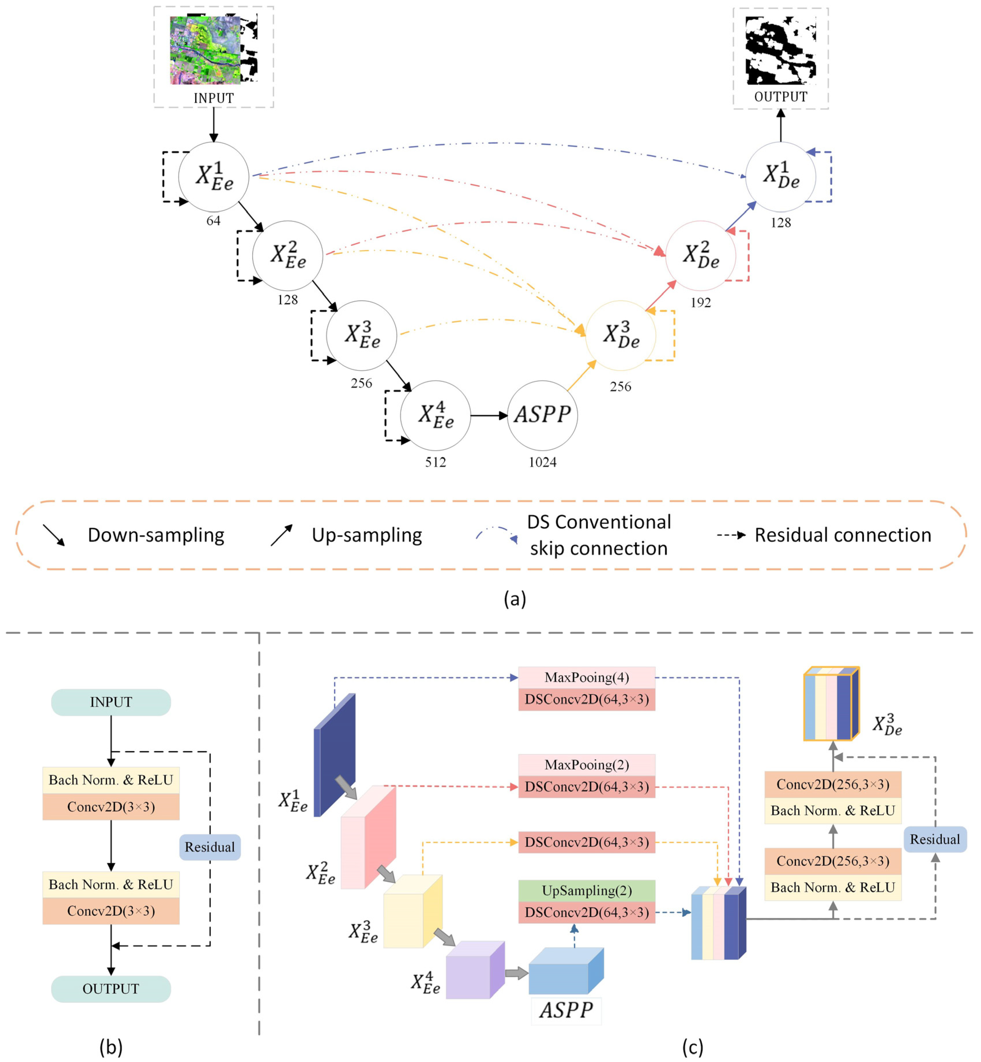
2.3. Network Architecture

This paper proposes an MSC-ResUNet network model that combines multiscale features through residual connections and multiscale skip connections, which effectively captures features ranging from low-level spatial details to high-level semantic information. The model further enhances performance by incorporating depthwise separable convolutions as part of the feature fusion process. The model structure is shown in Figure 5.

The encoder part includes four downsampling steps, featuring the following number of channels: (64, 128, 256, 512). Each step utilizes convolutional layers and residual connections [46] to enhance feature representation. The residual structure is illustrated in Figure 5b. In the bridging part between the encoder and decoder, MSC-ResUNet introduces an ASPP module with atrous rates of 1, 2, and 4. This choice is made considering the 30-m resolution of Landsat imagery, as larger atrous rates might result in overly sparse convolution kernels that fail to effectively capture fine-grained features. The ASPP module captures multiscale information and enhances the global receptive field of the feature maps.

The decoder part progressively restores spatial resolution through three upsampling steps, effectively integrating feature maps from different levels using multiscale skip connections and residual connections. The final decoder output is processed through a 1 × 1 convolutional layer and a sigmoid activation function to produce the final segmentation results.

2.3.1. Residual Blocks

In deep learning model design, residual blocks have become a widely used structure [47], especially in image segmentation tasks. Residual blocks introduce skip connections between layers, allowing gradients to propagate more effectively through the network. This mitigates common issues of gradient vanishing and gradient explosion in deep neural networks. The following equation demonstrates the working principle:

$$y_n=F\left(x_n,W_n\right)+x_n$$

(2)

where $x_n$ is the input and $F\left(·\right)$ is the residual function. This design not only accelerates the convergence speed of the network but also enhances the model’s feature learning capability. Through residual connections, the original input information is preserved and gradually transmitted between layers, enabling the network to retain original features while learning new ones. This improves the feature representation and resolution. The residual unit consists of various combinations of batch normalization (BN), ReLU, and convolutional layers. The residual structure in our model is shown in Figure 5b. Detailed descriptions of the combinations used and their effects can be found in the work of He [47].

2.3.2. Depthwise Separable Convolution

In the approach proposed by Chollet [48], standard convolution is decomposed into depthwise and pointwise convolutions, which are both separable depthwise. Depthwise convolution applies kernels independently to each channel, while pointwise convolution uses 1 × 1 convolutions across channels. This reduces parameters and computational cost, maintaining performance. Computational complexity decreases from $O\left(D_k^2·M·N·D_f^2\right)$ to $O\left(D_k^2·M·D_f^2+M·N{·D}_f^2\right)$, where $D_k$ is the kernel size, M and N are input and output channels, and $D_f$ is the feature map size. A structural diagram of the depth-separable convolution is visible in the Supplementary Material (Figure S1).

2.3.3. Multi-Scale Skip Connections

Our model uses multi-scale skip connections to transfer feature maps directly between the encoder and decoder, preserving high-resolution spatial information. Encoder output feature maps are processed through max pooling and depthwise separable convolutions before reaching the corresponding decoder layer, reducing parameters and computational cost. To bridge the semantic gap between the encoder and decoder, residual connections in the decoder add the encoder’s output directly to the decoder’s feature maps, enhancing stability and robustness.

The construction of the feature map of decoder layer $X_{De}^3$ is exemplified in Figure 5c. First, we merge feature maps from four scales. These four feature maps are obtained from: upsampling through bilinear interpolation to receive high-level semantic features from a deeper decoder layer, skip connections using depthwise separable convolution to receive feature maps from the same scale encoder layer $X_{Ee}^3$, and high-resolution spatial information feature maps from shallower encoder layers $X_{Ee}^2$ and $X_{Ee}^1$ processed by non-overlapping max pooling and depthwise separable convolution operations. During this process, we set the number of channels in all feature layers to 64 to simplify the model structure and improve computational efficiency. To merge shallow and deep information, we further perform residual convolution blocks on these four scales of concatenated feature maps, ensuring effective fusion of features from different levels. We define the multi-scale skip connection as follows: assuming i is the index of the encoder layer and N is the total number of encoders, the expression for $X_{De}^i$ as shown in Equation (3):

$$\begin{array}{c}\left\{\begin{array}{c}{X_{De}^i}^{\prime }=\left[{S\left(D\left(X_{Ee}^k\right)\right)}_{k=1}^{i-1},S\left(X_{Ee}^i\right),S\left(U\left(X_{Ee}^{i+1}\right)\right)\right], i=1,\cdots ,N-2\\ {X_{De}^i}^{\prime }=\left[{S\left(D\left(X_{Ee}^k\right)\right)}_{k=1}^{i-1},S\left(X_{Ee}^i\right),S\left(U\left(ASPP\right)\right)\right], i=N-1 \end{array}\right.\\ X_{De}^i=F\left({X_{De}^i}^{\prime },W_n\right)+{X_{De}^i}^{\prime },i=1,\cdots ,N-1\end{array}$$

(3)

where $S\left(·\right)$ represents the depthwise separable convolution operation, $D\left(·\right)$ represents the max pooling operation, $U\left(·\right)$ represents the upsampling operation, $\left[·\right]$ denotes the concatenation operation, ${X_{De}^i}^{\prime }$ represents the aggregated features after concatenation, and $F\left(·\right)$ is the residual function. $X_{De}^2$ and $X_{De}^1$ are generated in a similar manner. Therefore, the three upsampling steps feature the following number of channels: (256, 192, 128).

2.3.4. Dice Loss

Given the significant imbalance between background and cropland pixels in the training samples, this paper employs the Dice loss function. Derived from the Sørensen-Dice coefficient, Dice loss optimizes the overlap between the predicted and true segmentation, effectively addressing sample imbalance and providing a superior similarity measure, especially when the background class dominates, as shown in Equation (4):

$$Dice Coefficient=1-{\displaystyle \frac{2\left|A\cap B\right|}{\left|A\right|+\left|B\right|}}$$

(4)

where $\left|A\cap B\right|$ is the size of the intersection of predicted and true cropland pixels, and $\left|A\right|$ and $\left|B\right|$ are the sizes of the predicted and true cropland pixel sets, respectively.

2.3.5. Evaluation Metrics

To evaluate our model’s performance, we calculated Precision, Recall, F1-Score, and Matthews Correlation Coefficient (MCC), as shown in Equations (5)–(8). Precision measures the accuracy of positive predictions, while Recall assesses the model’s ability to identify actual positive samples. The F1-Score, the harmonic mean of Precision and Recall, provides a comprehensive performance evaluation. MCC, considering true positives, false positives, true negatives, and false negatives, offers a robust assessment, especially for imbalanced data. Additionally, a confusion matrix was analyzed to ensure a thorough evaluation of the model’s classification performance.

$$Precision={\displaystyle \frac{TP}{TP+FP}}$$

(5)

$$Recall={\displaystyle \frac{TP}{TP+FN}}$$

(6)

$$F1=2·{\displaystyle \frac{Precision\times Recall}{Precision+Recall}}$$

(7)

$$MCC={\displaystyle \frac{TP·TN-FP·FN}{\sqrt{\left(TP+FP\right)\left(TP+FN\right)\left(TN+FP\right)\left(TN+FN\right)}}}$$

(8)

where TP is the number of true positive samples, TN is the number of true negative samples, FP is the number of false positive samples, and FN is the number of false negative samples.

Our model was implemented using Keras 2.14 and TensorFlow 2.14.0, with CUDA 12.2, and was trained and evaluated on a workstation equipped with an NVIDIA Tesla V100 PCIe 32GB GPU. The optimizer used was Adam, with a cosine annealing learning rate restart strategy. The initial learning rate was set to 0.001, and it completed two cycles within each epoch, with the second cycle being twice the length of the first. Upon restarting, the learning rate was reset to 0.1 times the initial value, with a minimum learning rate of 0.0. Each model was trained for 100 epochs with a batch size of 8.

3. Results

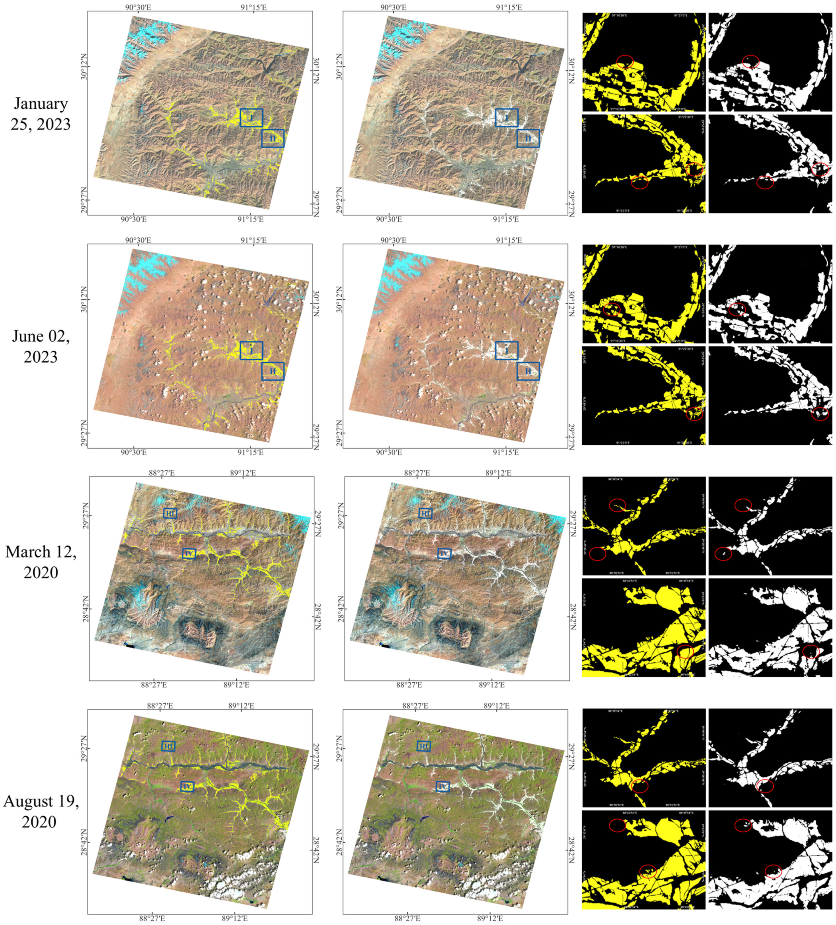
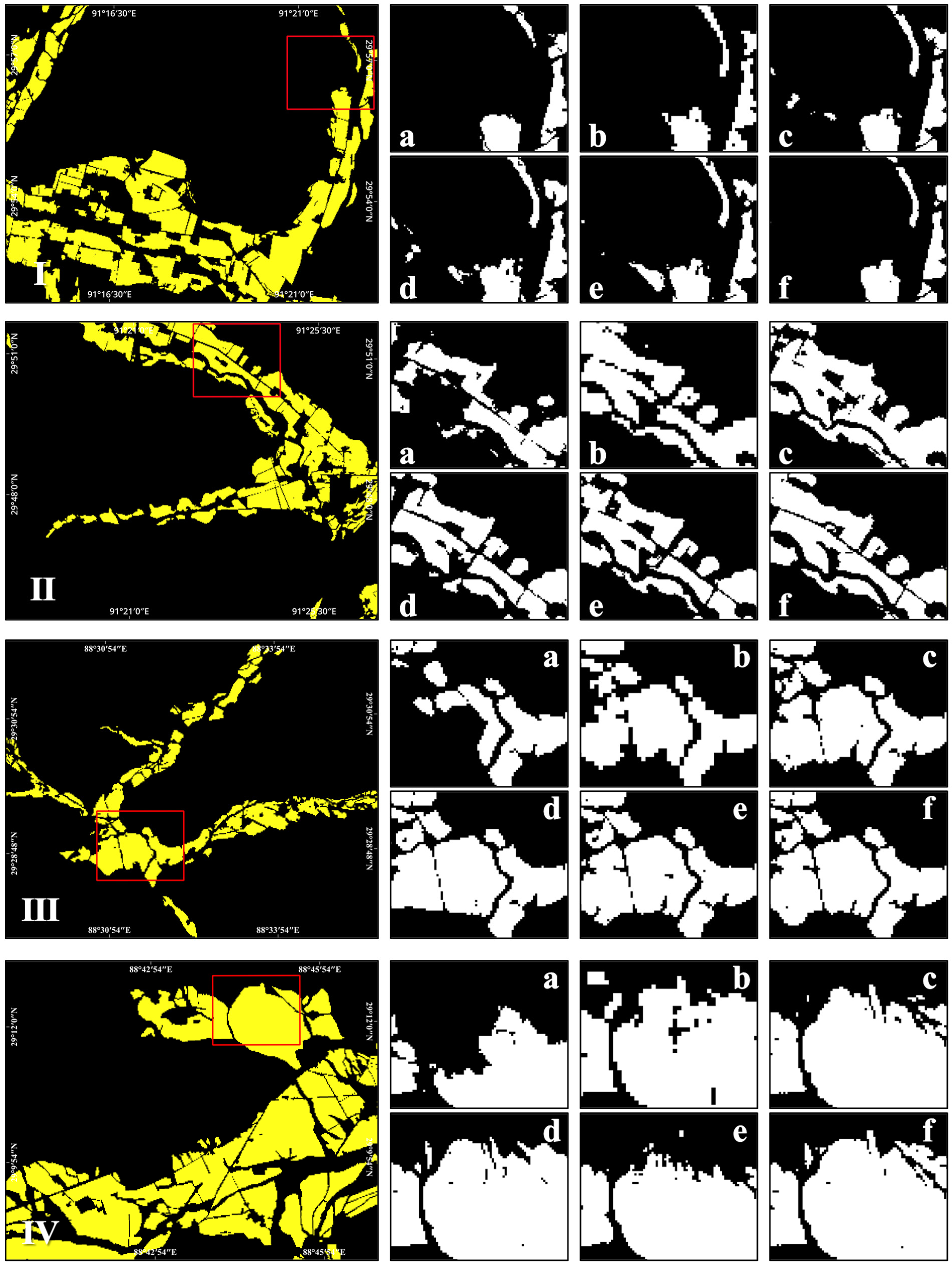
3.1. Performance of MSC-ResUNet

The MSC-ResUNet model was evaluated using both regional robustness and temporal transferability tests, with performance metrics summarized in

Table 2. Confusion matrix of MSC-ResUNet on the regional robustness validation dataset.

		Truth
		Cropland	Non-Cropland	Total	Precision
Prediction	Cropland	2,813,164	655,573	3,468,737	0.811
	Non-Cropland	530,335	55,507,616	56,037,951	0.991
	Total	3,343,499	56,163,189
	Recall	0.841	0.988
	MCC	0.8155
	F1	0.8259

and

Table 3. Confusion matrix of MSC-ResUNet on the temporal transferability validation dataset.

		Truth
		Cropland	Non-Cropland	Total	Precision
Prediction	Cropland	3,714,676	678,438	4,393,115	0.846
	Non-Cropland	570,082	67,978,372	68,548,453	0.992
	Total	4,284,758	68,656,810
	Recall	0.867	0.990
	MCC	0.8471
	F1	0.8561

. The model demonstrated high accuracy in both tests. In the regional robustness test, the MCC was 0.8155, and the F1 score was 0.8259, with cropland precision and recall at 0.811 and 0.841, respectively. In the temporal transferability test, the MCC was 0.8471 and the F1 score was 0.8561, with cropland precision and recall at 0.846 and 0.867. The prediction results for four images are presented, with local enlargements to display more details of the predicted results compared to the ground truth (Figure 6). Regions I and III in Figure 6 correspond to the locations in Figure 3A,B. These images are from two different periods within the same path and row numbers in the regional robustness test dataset and two different periods within the same path and row numbers in the temporal transferability test dataset. The results show that MSC-ResUNet effectively identified cropland pixels across different times and regions, with minimal misidentifications. Local enlargements in Figure 6 demonstrate the model’s high accuracy in identifying cropland pixels during different growth stages and in complex scenes, although a few small patches were misidentified, as indicated by red ellipses.

3.2. Comparison with Other Models

3.2.1. Performance Comparisons

The MSC-ResUNet model was compared with other deep learning models on the regional robustness and temporal transferability datasets. MSC-ResUNet outperforms the other comparison models, as shown in Figure 7. On the regional robustness dataset, compared to other models, the MCC of MSC-ResUNet improved by over 6.7%. Although HRNet performed closely, MSC-ResUNet still exceeded it by 2.3% in F1 score and 2.4% in MCC. On the temporal transferability dataset, most models demonstrated strong adaptability and consistency, with MCC values roughly close to or exceeding 0.8, indicating high accuracy in identifying cropland pixels and strong agreement between actual conditions and predictions. Specifically, the performance of MSC-ResUNet was also significantly better than that of other models, with an MCC of 0.8471 and an F1 score of 0.8561. The second-best performing model, HRNet, had an F1 score of 0.803 and an MCC of 0.791, which are 2.3% and 2.3% lower than those of MSC-ResUNet, respectively. The results are summarized in

Table 4. Performance of models on the regional robustness dataset and temporal transferability dataset.

Models	Regional Robustness Dataset				Temporal Transferability Dataset
	Precision	Recall	F1	MCC	Precision	Recall	F1	MCC
DeepLabv3+	0.727	0.676	0.701	0.684	0.812	0.763	0.786	0.774
UNet	0.668	0.847	0.747	0.736	0.842	0.778	0.809	0.798
ResUNet++	0.757	0.803	0.779	0.766	0.829	0.808	0.818	0.807
MACU-Net	0.735	0.792	0.763	0.749	0.782	0.850	0.815	0.804
HRNet	0.792	0.814	0.803	0.791	0.837	0.864	0.850	0.841
OURS	0.811	0.841	0.826	0.816	0.846	0.867	0.856	0.847

.

3.2.2. Model Parameters and Operational Efficiency

The parameter counts and the training and prediction operational efficiency of each model are shown in

Table 5. Comparison of model parameters and operational efficiency.

Model	Number of Parameters	FLOPs	Training (ms/Batch)	Prediction (ms/Batch)
DeepLabv3+	17,882,241 (68.22 MB)	5.82 G	198	105
UNet	31,058,693 (118.48 MB)	10.97 G	236	88
ResUNet++	101,994,116 (389.08 MB)	15.90 G	1015	111
MACU-Net	20,591,425 (78.55 MB)	13.49 G	299	93
HRNet	66,864,449 (255.07 MB)	16.76 G	508	181
OURS	35,261,697 (134.51 MB)	22.42 G	405	99

. Although the MSC-ResUNet has a parameter count of 35,261,697 (134.51 MB), which is not the smallest among all models, it demonstrates excellent training and prediction speeds, at 405 milliseconds per batch and 99 milliseconds per batch, respectively. In terms of computational complexity, MSC-ResUNet has a FLOPs value of 22.42 G, which, while higher than other models, does not hinder its operational efficiency. In comparison, HRNet, which has similar accuracy, has nearly twice the parameter count (255.07 MB) and a FLOPs value of 16.76 G, requiring more time for training and prediction. This indicates that MSC-ResUNet can achieve relatively fast computation speeds while maintaining high accuracy, making it suitable for tasks that require efficient and accurate processing of large-scale data.

4. Discussion

4.1. Ablation Study

Table 6. Ablation study.

No.	Main Model	ASPP	MSC		Precision	Recall	F1	MCC
			Conv	DS Conv
1	UNet				0.7924	0.8250	0.8084	0.7969
2	UNet				0.7917	0.8265	0.8087	0.7973
3	UNet	✓		✓	0.7891	0.8350	0.8114	0.8002
4	ResUNet				0.7752	0.8247	0.7992	0.7873
5	ResUNet			✓	0.8062	0.8386	0.8221	0.8114
6	ResUNet	✓	✓		0.7807	0.7976	0.7891	0.7764
7	ResUNet	✓		✓	0.8110	0.8414	0.8259	0.8155

presents an ablation study analyzing the impact of various modules on the model’s performance, including multi-scale skip connections, ASPP, and residual connection modules. The key findings are as follows: (1) Comparing Model 3 with Model 2, Precision slightly decreased while Recall significantly improved. Similarly, Model 5 showed noticeable improvements over Model 4 in all metrics, indicating that MSC effectively fuses features at different scales, enhancing Recall and overall performance. (2) Comparing the results of Model 7 with Model 6, replacing the standard convolution in full-scale skip connections with depthwise separable convolution significantly improved all metrics. This demonstrates that depthwise separable convolution further enhances the effectiveness of MSC, reducing computational load while improving feature extraction and fusion performance. (3) Comparing Model 1 with Model 4, the addition of the residual module alone resulted in minor performance changes. This suggests that the residual connection module alone has limited impact on metrics but may stabilize the model during training by providing better gradient flow. (4) The results of Models 1, 4–5, and 7 show that gradually adding the residual connection module, using MSC with depthwise separable convolutions, and incorporating ASPP modules improves the model’s performance. F1 scores increased by 0.92%, 1.37%, and 1.75%, respectively. The combination of all modules performed best across all metrics, indicating that the integration of the residual connection module, MSC with depthwise separable convolutions, and ASPP modules significantly enhances the model’s predictive performance.

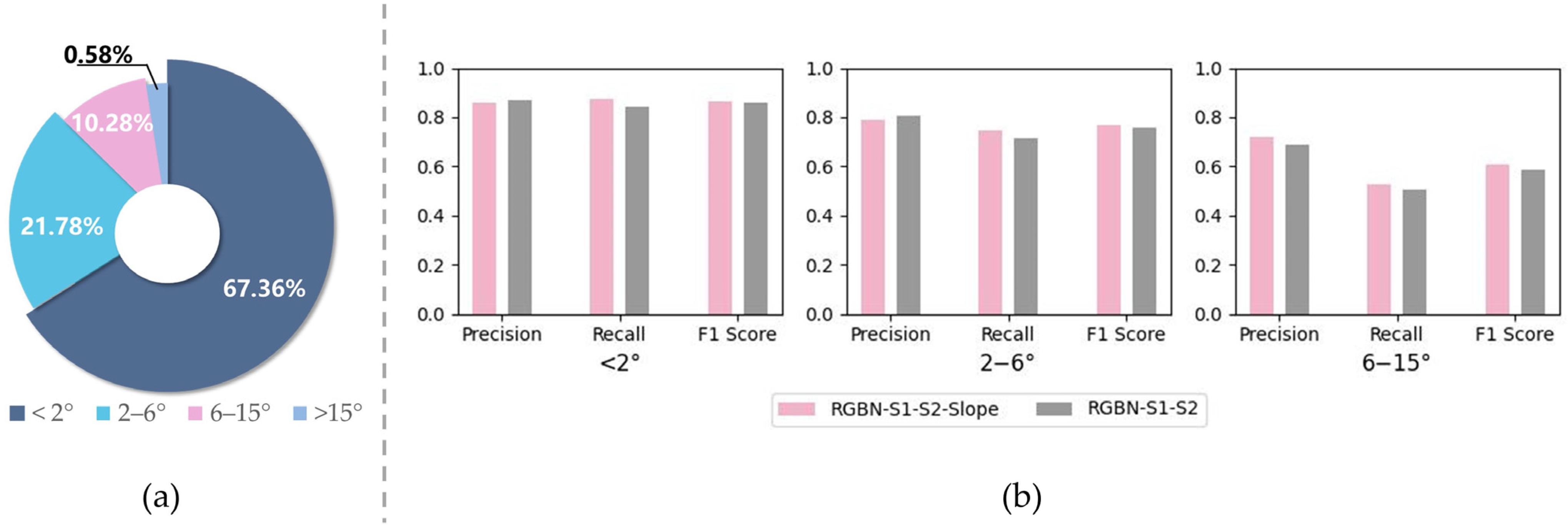
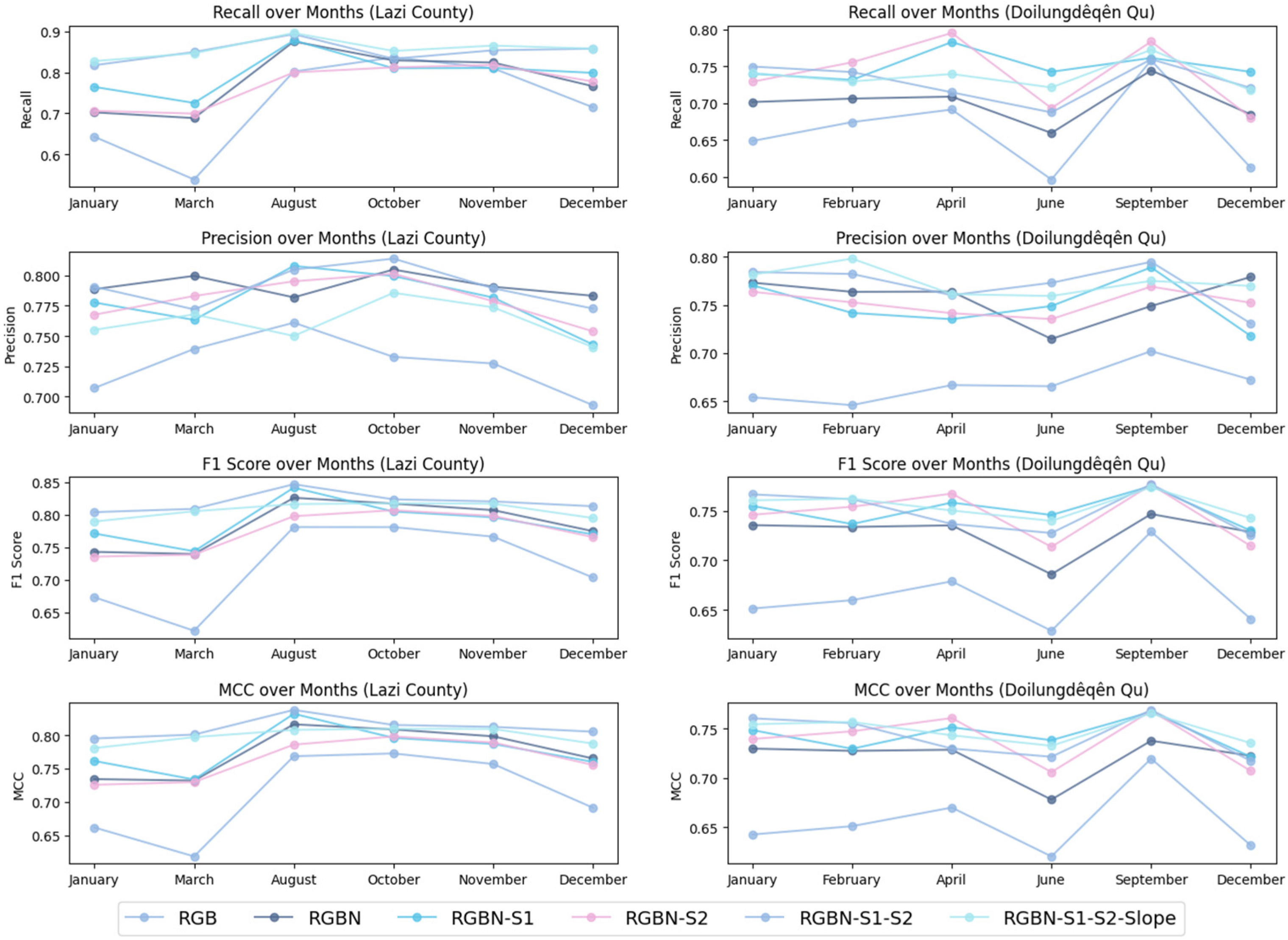
4.2. The Adaptability of the Model to Different Band Combinations

Landsat 8 is a multispectral sensor, and different band combinations can affect the performance of cropland identification. Here, we selected different band combinations as input training data to evaluate the performance of the MSC-ResUNet model, especially on the regional robustness dataset. Specifically, the types of band combinations used are shown in

Table 7. Band combinations used in the study.

Band Combinations	Used Bands
RGB	true-color channels. (OLI band 2–4)
RGBN	true-color channels, near-infrared channel. (OLI band 2–5)
RGBN-S1	true-color channels, near-infrared channel, short-wave infrared 1. (OLI band 2–6)
RGBN-S2	true-color channels, near-infrared channel, short-wave infrared 2. (OLI band 2–5, 7)
RGBN-S1-S2	true-color channels, near-infrared channel, short-wave infrared 1, short-wave infrared 2. (OLI band 2–7)
RGBN-S1-S2-Slope	true-color channels, near-infrared channel, short-wave infrared 1, short-wave infrared 2, slope.

.

Table 8. Performance of MSC-ResUNet model with different Landsat band combinations on the regional robustness dataset.

Band Combinations	Metrics
	Precision	Recall	F1	MCC
RGB	0.732	0.730	0.7314	0.7155
RGBN	0.798	0.755	0.7757	0.7630
RGBN-S1	0.796	0.809	0.8023	0.7904
RGBN-S2	0.805	0.779	0.7920	0.7799
RGBN-S1-S2	0.814	0.810	0.8120	0.8009
RGBN-S1-S2-Slope	0.811	0.841	0.8259	0.8155

presents the performance metrics for different band combinations. The basic RGB combination performed poorly across all metrics, with an MCC of 0.715. When the near-infrared band was added, performance improved markedly, raising the MCC to 0.763. Further inclusion of the shortwave infrared bands continued to enhance performance, particularly in the RGBN-SWIR1-SWIR2 combination, where the F1 score reached 0.812 and the MCC reached 0.801. Adding slope information improved recall significantly, achieving the best overall performance with an MCC of 0.816, despite a slight decrease in precision.

The addition of different band combinations significantly enhances MSC-ResUNet performance due to the distinct spectral differences between vegetation and other land features in the near-infrared to shortwave infrared bands. The enhancement effect becomes more pronounced as the number of bands increases. When slope information is added, precision decreases while recall increases. This can be attributed to the significant terrain variations and fragmented cropland distribution in the study area on the Qinghai-Tibet Plateau.

According to the “Technical Regulations for the Third National Land Survey” issued by the Ministry of Natural Resources of the People’s Republic of China, cropland slope is classified into five grades: ≤2°, 2−6°, 6−15°, 15−25°, and greater than 25°. The spatial distribution of cropland in the slope categories of the regional robustness validation dataset was as follows: 67.36%, 21.78%, 8.39%, 0.51%, and 0.03%, as shown in Figure 8a.

We further explored the impact of adding slope information on model performance in different slope ranges, focusing on areas with slopes ≤2°, 2−6°, and 6−15° (Figure 8b). In areas with slopes ≤2°, the inclusion of slope information does not result in significant changes in precision, recall, or F1 score, indicating that the overall classification performance is not strongly influenced by the slope in flat areas. However, in regions with slopes of 2–6°, the model’s recall improves significantly with the addition of slope information, though precision decreases slightly, suggesting that slope data helps in identifying more cropland areas in moderately sloped regions, though at the cost of introducing some false positives. In steeper regions with slopes of 6–15°, there is a notable improvement in precision, recall, and F1 scores, indicating that slope data is particularly beneficial in more challenging terrain. In conclusion, slope information enhances the model’s ability to generalize across varying terrains, especially in regions with moderate slopes. However, in flatter regions, the effect of adding slope data is limited, potentially leading to a slight increase in false positives due to the misclassification of non-cropland areas with similar spectral characteristics.

Experimental results indicate that high performance is achieved with combinations including RGB, near-infrared, and any shortwave infrared band, suggesting that these bands provide crucial spectral information. Under limited computational resources, using RGB and near-infrared bands, or combinations including shortwave infrared bands, can achieve good results with lower data volumes, reducing computational costs and improving practical applicability.

4.3. The Adaptability of the Model to Different Time Phases of Satellite Data

To further explore the impact of different band combinations across different months, Doilungdêqên Qu and Lazi County within the robustness dataset testing areas of path and row numbers 138/039 and 140/040, respectively, were selected. The results are shown in Figure 9. The main crops in Doilungdêqên Qu include barley, spring wheat, and winter wheat, and Lazi County include barley, spring wheat, peas, and forage. Figure 10 presents the mean and standard deviation of surface reflectance for cropland in both regions across different months, showing significant spectral differences at certain times. The spectral reflectance statistics are derived from Landsat data, utilizing points from the previously discussed cropland validation dataset. These validation points are representative of the cropland in their respective regions. From April to September, most metrics performed better compared to other months, particularly in August and September, where the F1 and MCC values in both regions reached their highest levels. However, in June, the metrics for Doilungdêqên Qu showed a noticeable decline due to extensive cloud cover over the cropland. Interestingly, the model’s performance did not significantly decline in non-growing seasons, sometimes even surpassing growing season performance under certain band combinations. This indicates that the model successfully learned the features of non-growing season cropland, enabling effective cropland identification year-round.

4.4. Advantages and Limitations

MSC-ResUNet model effectively integrates multiscale features through residual connections and MSC, capturing both low-level spatial and high-level semantic features. In both the regional robustness and temporal transferability tests, MSC-ResUNet demonstrated high accuracy and strong adaptability across different regions and time periods. Additionally, MSC-ResUNet showed excellent training and prediction speeds, suitable for tasks requiring efficient processing of large-scale data.

However, despite its high computational efficiency, the model’s parameter counts of 35,261,697 (134.51 MB) could be a constraint in resource-limited environments. Future research should focus on optimizing data processing and model structure to enhance the model’s robustness and adaptability.

5. Conclusions

This paper proposes an MSC-ResUNet network model that enhances feature fusion by introducing depthwise separable convolutions in multiscale skip connections and residual connections in the decoder part, which aims to improve the accuracy of fractured cropland extraction using 30-m resolution Landsat multi-band data. Additionally, due to the lack of high-quality training datasets for the “One River, Two Streams” region of the Qinghai-Tibet Plateau, we independently created a high-quality pixel-level precision training dataset. This provides a solid foundation for cropland mapping using Landsat data combined with deep learning.

MSC-ResUNet demonstrated excellent performance across different scenarios and time periods through regional robustness and temporal transferability tests. In the regional robustness test, MSC-ResUNet achieved an MCC of 0.8155 and an F1 score of 0.8259, showcasing its superiority in handling complex land cover conditions. In the temporal transferability test, the model achieved an MCC of 0.8471 and an F1 score of 0.8561, indicating strong adaptability and consistency across different time periods. Experiments with different band combinations and different months showed that the inclusion of near-infrared, shortwave infrared, and slope information significantly enhanced model performance. With limited computational resources, using combinations of RGB and near-infrared bands, or including shortwave infrared bands, can achieve good results with lower data volumes, reducing computational costs and improving practicality. Additionally, the model demonstrated satisfactory accuracy in both the growing season and non-growing season imagery, exhibiting consistent and reliable extraction results across diverse months and complex land cover conditions, which highlights the model’s adaptability and robustness.

Overall, MSC-ResUNet excels in handling complex land cover and low-resolution imagery by combining multiscale features and optimized band combinations, significantly improving segmentation accuracy and model robustness. Future research could consider using other satellite data with similar resolutions to increase observation frequency, thereby reducing weather-related image interference and improving data timeliness and continuity. Additionally, further optimization of data processing and model structure could reduce the model’s parameter count.

References

1. Giri, C.P. Remote Sensing of Land Use and Land Cover: Principles and Applications; CRC Press: Boca Raton, FL, USA, 2012; ISBN 978-1-4200-7074-3. [Google Scholar]
2. Badreldin, N.; Abu Hatab, A.; Lagerkvist, C.-J. Spatiotemporal Dynamics of Urbanization and Cropland in the Nile Delta of Egypt Using Machine Learning and Satellite Big Data: Implications for Sustainable Development. Environ. Monit. Assess. 2019, 191, 767. [Google Scholar] [CrossRef]
3. Corgne, S.; Hubert-Moy, L.; Betbeder, J. Monitoring of Agricultural Landscapes Using Remote Sensing Data. In Land Surface Remote Sensing in Agriculture and Forest; Baghdadi, N., Zribi, M., Eds.; Elsevier: Amsterdam, The Netherlands, 2016; pp. 221–247. ISBN 978-1-78548-103-1. [Google Scholar]
4. Hamud, A.M.; Prince, H.M.; Shafri, H.Z. Landuse/Landcover Mapping and Monitoring Using Remote Sensing and GIS with Environmental Integration. IOP Conf. Ser. Earth Environ. Sci. 2019, 357, 012038. [Google Scholar] [CrossRef]
5. Wang, X.; Shu, L.; Han, R.; Yang, F.; Gordon, T.; Wang, X.; Xu, H. A Survey of Farmland Boundary Extraction Technology Based on Remote Sensing Images. Electronics 2023, 12, 1156. [Google Scholar] [CrossRef]
6. Xia, L.; Zhao, F.; Chen, J.; Yu, L.; Lu, M.; Yu, Q.; Liang, S.; Fan, L.; Sun, X.; Wu, S.; et al. A Full Resolution Deep Learning Network for Paddy Rice Mapping Using Landsat Data. ISPRS-J. Photogramm. Remote Sens. 2022, 194, 91–107. [Google Scholar] [CrossRef]
7. Julien, Y.; Sobrino, J.A.; Jiménez-Muñoz, J.-C. Land Use Classification from Multitemporal Landsat Imagery Using the Yearly Land Cover Dynamics (YLCD) Method. Int. J. Appl. Earth Obs. Geoinf. 2011, 13, 711–720. [Google Scholar] [CrossRef]
8. Ortiz, M.J.; Formaggio, A.R.; Epiphanio, J.C.N. Classification of Croplands through Integration of Remote Sensing, GIS, and Historical Database. Int. J. Remote Sens. 1997, 18, 95–105. [Google Scholar] [CrossRef]
9. Teluguntla, P.; Thenkabail, P.S.; Oliphant, A.; Xiong, J.; Gumma, M.K.; Congalton, R.G.; Yadav, K.; Huete, A. A 30-m Landsat-Derived Cropland Extent Product of Australia and China Using Random Forest Machine Learning Algorithm on Google Earth Engine Cloud Computing Platform. ISPRS J. Photogramm. Remote Sens. 2018, 144, 325–340. [Google Scholar] [CrossRef]
10. Wardlow, B.D.; Egbert, S.L. Large-Area Crop Mapping Using Time-Series MODIS 250 m NDVI Data: An Assessment for the U.S. Central Great Plains. Remote Sens. Environ. 2008, 112, 1096–1116. [Google Scholar] [CrossRef]
11. Xiao, X.; Boles, S.; Liu, J.; Zhuang, D.; Frolking, S.; Li, C.; Salas, W.; Moore, B. Mapping Paddy Rice Agriculture in Southern China Using Multi-Temporal MODIS Images. Remote Sens. Environ. 2005, 95, 480–492. [Google Scholar] [CrossRef]
12. Zhang, G.; Xiao, X.; Dong, J.; Kou, W.; Jin, C.; Qin, Y.; Zhou, Y.; Wang, J.; Menarguez, M.A.; Biradar, C. Mapping Paddy Rice Planting Areas through Time Series Analysis of MODIS Land Surface Temperature and Vegetation Index Data. ISPRS J. Photogramm. Remote Sens. 2015, 106, 157–171. [Google Scholar] [CrossRef]
13. Walker, J.J.; de Beurs, K.M.; Wynne, R.H. Dryland Vegetation Phenology across an Elevation Gradient in Arizona, USA, Investigated with Fused MODIS and Landsat Data. Remote Sens. Environ. 2014, 144, 85–97. [Google Scholar] [CrossRef]
14. Dong, J.; Xiao, X.; Kou, W.; Qin, Y.; Zhang, G.; Li, L.; Jin, C.; Zhou, Y.; Wang, J.; Biradar, C.; et al. Tracking the Dynamics of Paddy Rice Planting Area in 1986–2010 through Time Series Landsat Images and Phenology-Based Algorithms. Remote Sens. Environ. 2015, 160, 99–113. [Google Scholar] [CrossRef]
15. Wang, Q.; Guo, P.; Dong, S.; Liu, Y.; Pan, Y.; Li, C. Extraction of Cropland Spatial Distribution Information Using Multi-Seasonal Fractal Features: A Case Study of Black Soil in Lishu County, China. Agriculture 2023, 13, 486. [Google Scholar] [CrossRef]
16. Yang, R.; He, G.; Yin, R.; Wang, G.; Zhang, Z.; Long, T.; Peng, Y. Weakly-Semi Supervised Extraction of Rooftop Photovoltaics from High-Resolution Images Based on Segment Anything Model and Class Activation Map. Appl. Energy 2024, 361, 122964. [Google Scholar] [CrossRef]
17. Peng, X.; He, G.; Wang, G.; Yin, R.; Wang, J. A Weakly Supervised Semantic Segmentation Framework for Medium-Resolution Forest Classification with Noisy Labels and GF-1 WFV Images. IEEE Trans. Geosci. Remote Sens. 2024, 62, 4412419. [Google Scholar] [CrossRef]
18. Shunying, W.; Ya’nan, Z.; Xianzeng, Y.; Li, F.; Tianjun, W.; Jiancheng, L. BSNet: Boundary-Semantic-Fusion Network for Farmland Parcel Mapping in High-Resolution Satellite Images. Comput. Electron. Agric. 2023, 206, 107683. [Google Scholar] [CrossRef]
19. Li, C.; Fu, L.; Zhu, Q.; Zhu, J.; Fang, Z.; Xie, Y.; Guo, Y.; Gong, Y. Attention Enhanced U-Net for Building Extraction from Farmland Based on Google and WorldView-2 Remote Sensing Images. Remote Sens. 2021, 13, 4411. [Google Scholar] [CrossRef]
20. Lipton, Z.C.; Berkowitz, J.; Elkan, C. A Critical Review of Recurrent Neural Networks for Sequence Learning. arXiv 2015, arXiv:1506.00019. [Google Scholar]
21. Hochreiter, S.; Schmidhuber, J. Long Short-Term Memory. Neural Comput. 1997, 9, 1735–1780. [Google Scholar] [CrossRef]
22. Lin, Z.; Zhong, R.; Xiong, X.; Guo, C.; Xu, J.; Zhu, Y.; Xu, J.; Ying, Y.; Ting, K.C.; Huang, J.; et al. Large-Scale Rice Mapping Using Multi-Task Spatiotemporal Deep Learning and Sentinel-1 SAR Time Series. Remote Sens. 2022, 14, 699. [Google Scholar] [CrossRef]
23. Xu, J.; Yang, J.; Xiong, X.; Li, H.; Huang, J.; Ting, K.C.; Ying, Y.; Lin, T. Towards Interpreting Multi-Temporal Deep Learning Models in Crop Mapping. Remote Sens. Environ. 2021, 264, 112599. [Google Scholar] [CrossRef]
24. Zhong, L.; Hu, L.; Zhou, H. Deep Learning Based Multi-Temporal Crop Classification. Remote Sens. Environ. 2019, 221, 430–443. [Google Scholar] [CrossRef]
25. Badrinarayanan, V.; Kendall, A.; Cipolla, R. SegNet: A Deep Convolutional Encoder-Decoder Architecture for Image Segmentation. IEEE Trans. Pattern Anal. Mach. Intell. 2017, 39, 2481–2495. [Google Scholar] [CrossRef]
26. Ronneberger, O.; Fischer, P.; Brox, T. U-Net: Convolutional Networks for Biomedical Image Segmentation. In Medical Image Computing and Computer-Assisted Intervention–MICCAI 2015: 18th International Conference, Munich, Germany, 5–9 October 2015; Springer: Cham, Switzerland, 2015. [Google Scholar]
27. Sathyanarayanan, D.; Anudeep, D.; Keshav Das, C.A.; Bhanadarkar, S.; Uma, D.; Hebbar, R.; Raj, K.G. A Multiclass Deep Learning Approach for LULC Classification of Multispectral Satellite Images. In Proceedings of the 2020 IEEE India Geoscience and Remote Sensing Symposium (InGARSS), Ahmedabad, India, 1–4 December 2020; pp. 102–105. [Google Scholar]
28. Zaheer, S.A.; Ryu, Y.; Lee, J.; Zhong, Z.; Lee, K. In-Season Wall-to-Wall Crop-Type Mapping Using Ensemble of Image Segmentation Models. IEEE Trans. Geosci. Remote Sens. 2023, 61, 4411311. [Google Scholar] [CrossRef]
29. Qu, Y.; Zhang, B.; Xu, H.; Qiao, Z.; Liu, L. Interannual Monitoring of Cropland in South China from 1991 to 2020 Based on the Combination of Deep Learning and the LandTrendr Algorithm. Remote Sens. 2024, 16, 949. [Google Scholar] [CrossRef]
30. Huang, H.; Lin, L.; Tong, R.; Hu, H.; Zhang, Q.; Iwamoto, Y.; Han, X.; Chen, Y.-W.; Wu, J. UNet 3+: A Full-Scale Connected UNet for Medical Image Segmentation. In Proceedings of the ICASSP 2020—2020 IEEE International Conference on Acoustics, Speech and Signal Processing (ICASSP), Barcelona, Spain, 4–8 May 2020; IEEE: Piscataway, NJ, USA, 2020; pp. 1055–1059. [Google Scholar]
31. Zhou, Z.; Siddiquee, M.M.R.; Tajbakhsh, N.; Liang, J. UNet++: A Nested U-Net Architecture for Medical Image Segmentation. In Deep Learning in Medical Image Analysis and Multimodal Learning for Clinical Decision Support; Springer: Berlin/Heidelberg, Germany, 2018. [Google Scholar]
32. Li, R.; Duan, C.; Zheng, S.; Zhang, C.; Atkinson, P.M. MACU-Net for Semantic Segmentation of Fine-Resolution Remotely Sensed Images. IEEE Geosci. Remote Sens. Lett. 2022, 19, 8007205. [Google Scholar] [CrossRef]
33. Bejani, M.M.; Ghatee, M. A Systematic Review on Overfitting Control in Shallow and Deep Neural Networks. Artif. Intell. Rev. 2021, 54, 6391–6438. [Google Scholar] [CrossRef]
34. Sun, Z.; Li, L.; Liu, Y.; Du, X.; Li, L. On the Importance of Building High-Quality Training Datasets for Neural Code Search. In Proceedings of the 44th International Conference on Software Engineering, Pittsburgh, PA, USA, 21–29 May 2022. [Google Scholar]
35. Zheng, K.; He, G.; Yin, R.; Wang, G.; Long, T. A Comparison of Seven Medium Resolution Impervious Surface Products on the Qinghai–Tibet Plateau, China from a User’s Perspective. Remote Sens. 2023, 15, 2366. [Google Scholar] [CrossRef]
36. Guo, Y.; HUANG, Z.; DU, J. Variation characteristics of agricultural boundary temperature in main agricultural regions in basins of the Brahmaputra River and its two tributaries in Xizang from 1981 to 2022. Arid Meteorol. 2024, 42, 47–53. [Google Scholar]
37. Li, D.; Tian, P.; Luo, H. Spatio-Temporal Characteristics and Obstacle Diagnosis of Cultivated Land Ecological Security in “One River and Two Tributaries” Region in Tibet. Trans. Chin. Soc. Agric. Mach. 2020, 51, 10. [Google Scholar] [CrossRef]
38. Liu, G.; Nimazhaxi; Song, G.; Cheng, L. Analysis of Soil Nutrients Limiting Factors for Barley Production in Centre Tibet. Chin. J. Agrometeorol. 2014, 35, 276–280. [Google Scholar]
39. Wu, F.; Ma, W.; Li, T.; Yan, X.; Ma, X.; Tang, S.; Zhang, F. Spatiotemporal patterns and other impacting factors on wheat production of Tibet, China. Chin. J. Appl. Environ. Biol. 2022, 28, 945–953. [Google Scholar] [CrossRef]
40. Huang, L.; Feng, Y.; Zhang, B.; Hu, W. Spatio-Temporal Characteristics and Obstacle Factors of Cultivated Land Resources Security. Sustainability 2021, 13, 8498. [Google Scholar] [CrossRef]
41. Bai, W.; Yao, L.; Zhang, Y.; Wang, C. Spatial-temporal Dynamics of Cultivated Land in Recent 35 Years in the Lhasa River Basin of Tibet. J. Nat. Resour. 2014, 29, 623–632. [Google Scholar]
42. Tao, J.; Wang, Y.; Liu, F.; Zhang, Y.; Chen, Q.; Wu, L. Identification and determination of its critical values for influencing factors of cultivated land reclamation strength in region of Brahmaputra River and its two tributaries in Tibet. Trans. Chin. Soc. Agric. Eng. 2016, 32, 239–246. [Google Scholar] [CrossRef]
43. Liu, J.; Yu, Z. The Study and Practice on the Application of Colour Infrared Aerial Remote Sensing Technique to Non-cultivation Coefficient Calculation in Tibet. Natl. Remote Sens. Bull. 1990, 5, 27–37+81. [Google Scholar]
44. Van De Kerchove, R.; Zanaga, D.; Keersmaecker, W.; Souverijns, N.; Wevers, J.; Brockmann, C.; Grosu, A.; Paccini, A.; Cartus, O.; Santoro, M.; et al. ESA WorldCover: Global Land Cover Mapping at 10 m Resolution for 2020 Based on Sentinel-1 and 2 Data. In Proceedings of the AGU Fall Meeting Abstracts, New Orleans, LA, USA, 13–17 December 2021; Volume 2021, p. GC45I-0915. [Google Scholar]
45. Chen, J.; Zhang, J.; Zhang, W.; Peng, S. Continous Updating and Refinement of Land Cover Data Product. J. Remote Sens. 2016, 20, 991–1001. [Google Scholar] [CrossRef]
46. He, K.; Zhang, X.; Ren, S.; Sun, J. Deep Residual Learning for Image Recognition. In Proceedings of the IEEE Conference on Computer Vision and Pattern Recognition (CVPR), Boston, MA, USA, 7–12 June 2015. [Google Scholar]
47. He, K.; Zhang, X.; Ren, S.; Sun, J. Identity Mappings in Deep Residual Networks. In Proceedings of the Computer Vision–ECCV 2016: 14th European Conference, Amsterdam, The Netherlands, 11–14 October 2016. [Google Scholar]
48. Chollet, F. Xception: Deep Learning with Depthwise Separable Convolutions. In Proceedings of the IEEE Conference on Computer Vision and Pattern Recognition, Honolulu, HI, USA, 21–26 July 2017. [Google Scholar]
Figure 1. The workflow of the study.
Remotesensing 16 04071 g001
Figure 2. Location of the study area. (A) shows the schematic representation of the location of the YarlungZangbo-Lhasa-Nyangqv River region within the Qinghai-Tibet Plateau. (B) displays the distribution of cropland in the YarlungZangbo-Lhasa-Nyangqv River region in 2023, with cropland indicated in black. (C) illustrates the distribution of Landsat scenes, with numbers representing path and row for Landsat 8 scenes.
Remotesensing 16 04071 g002
Figure 3. (A,B) represent Gaofen-1 imagery from 2 September 2023 and Gaofen-6 imagery from 17 May 2020, respectively. (A1A3) show true-color Landsat 8 images from 15 April, 2 June and 6 September 2023, respectively. Similarly, (B1B3) depict true-color Landsat 8 images from 12 March, 19 August and 4 September 2020. (a,b) illustrate the corresponding cropland label samples, with the cropland areas highlighted in yellow.
Remotesensing 16 04071 g003
Figure 4. The distribution map of validation samples in the study area. (ad) represent true-color cropland images with a 2-m resolution from Gaofen-1, captured on 14 May, 7 June, 14 September and 27 September 2023. Yellow points indicate cropland validation points derived from manual interpretation, while blue points represent non-cropland validation points.
Remotesensing 16 04071 g004
Figure 5. The overall structure of the MSC-ResUNet. (a) shows the overall architecture of the model, including the depth of each layer in the encoder and decoder, with depth information labeled below each circular node; (b) illustrates the residual connection structure in the encoder part; (c) using X D e 3 explains the specific application of multi-scale skip connections and residual connections in the decoder layers.
Remotesensing 16 04071 g005
Figure 6. The prediction results of MSC-ResUNet for images from 25 January 2023, 2 June 2023, 12 March 2020, and 19 August 2020, along with the enlarged views of the corresponding regions indicated by blue boxes I–IV. Yellow pixels represent true cropland, black represents non-cropland, and white represents predicted cropland. Red ellipses indicate misidentified patches.
Remotesensing 16 04071 g006
Figure 7. Zoom-in of the predicted results: (IIV) represent the ground truth for 25 January 2023, 2 June 2023, 12 March 2020, and 19 August 2020, respectively. The red squares in (IIV) indicate the regions for which the prediction results are shown in (af), showing the prediction results from DeepLabv3+, HRNet, MACU-Net, UNet, ResUNet++, and MSC-RESUNET, respectively.
Remotesensing 16 04071 g007
Figure 8. (a) shows the spatial distribution of cropland in the slope categories of the regional robustness validation dataset. (b) displays the slope information on model performance in different slope ranges.
Remotesensing 16 04071 g008
Figure 9. Performance of MSC-ResUNet with different band combinations across various months.
Remotesensing 16 04071 g009
Figure 10. Spectral reflectance time series of cropland in Lazi County and Doilungdêqên Qu. The mean and standard deviation are represented by lines and error bars, respectively.
Remotesensing 16 04071 g010