Infrared Small Target Detection Based on Weighted Improved Double Local Contrast Measure

Abstract

The robust detection of infrared small targets plays an important role in infrared early warning systems. However, the high-brightness interference present in the background makes it challenging. To solve this problem, we propose a weighted improved double local contrast measure (WIDLCM) algorithm in this paper. Firstly, we utilize a fixed-scale three-layer window to compute the double neighborhood gray difference to screen candidate target pixels and estimate the target size. Then, according to the size information of each candidate target pixel, an improved double local contrast measure (IDLCM) based on the gray difference is designed to enhance the target and suppress the background. Next, considering the structural characteristics of the target edge, we propose the variance-based weighting coefficient to eliminate clutter further. Finally, the targets are detected by an adaptive threshold. Extensive experimental results demonstrate that our method outperforms several state-of-the-art methods.

1. Introduction

Infrared small target detection with a high detection rate and low false-alarm rate is crucial in early warning and precise guidance. Due to the long detection distance, the target usually occupies a few pixels in the image and has little shape and texture information. Meanwhile, in practical applications, there is often high-brightness clutter in the background. These obstacles make it difficult for small targets to be accurately detected in various complex scenarios.

In the past few years, numerous infrared small target detection methods were proposed, which can be categorized into single-frame-based and sequence-based methods. Single-frame detection methods require less data and consume less time than sequential detection methods. Therefore, our research focused on single-frame detection methods.

Early detection algorithms estimate the background by spatial filtering and subtract the background from the original image to extract small targets, like the max-mean/max-median filters [1]. These methods are efficient in simple backgrounds but struggle to deal with complex backgrounds. Some algorithms use morphological filters. Bai et al. [2] proposed a new top-hat transformation using two different but related structural elements. Deng et al. [3] built an adaptive ring structural element based on the M-estimator and used a novel local entropy to weight it. Wang et al. [4] designed eight nonconcentric ring structural elements to enhance small targets in different directions. Li et al. [5] constructed an adaptive ring-shaped structural element based on the difference-of-structure tensors to capture local features for background estimation.

The object detection task has also been transformed into an optimization problem of recovering low-rank and sparse matrices, first proposed by Gao et al. [6]. Dai et al. [7] proposed a reweighted infrared patch-tensor model using both local and non-local priors. In order to more accurately represent the background rank and be more attuned to noise, Kong et al. [8] proposed an improved IPT model based on a nonconvex tensor fibered rank approximation. Zhao et al. [9] designed corner and edge weights to avoid strong edge interference being mistaken for targets. These methods based on iterative optimization are time-consuming and difficult to apply in practice [10].

Based on the assumption that targets are isotropic, detection algorithms utilizing directional derivatives or gradients were proposed. Zhang et al. [11] constructed the infrared gradient vector field (IGVF) of the original image using a facet model and then used a gradient correlation template to traverse the IGVF map to calculate the correlation. Liu et al. [12] calculated multidirectional derivatives based on the facet model and screened the candidate target points to improve the detection speed.

The detection methods based on deep learning have also achieved great success. Dai et al. [13] proposed the ALCNet, which introduced the attention mechanism to preserve the features of small targets better. Hou et al. [14] used the U-shaped deep neural network for infrared small target detection, converting the input image into a target probability likelihood map. Chen et al. [15] proposed a multi-task model that combines semantic segmentation and target detection. Li et al. [16] proposed the dense nested attention network (DNA-Net) to prevent target loss in the deep layers of the network. However, such detection methods often require rich infrared images and manual annotation, which limit their practicality in various scenarios.

In recent years, local contrast methods based on the human visual system (HVS) have attracted the attention of researchers. The infrared small target detection algorithm based on local contrast was first proposed by Chen et al. [17] to calculate the contrast measure between the maximum gray value of the central cell and the maximum mean gray value of the neighboring cells of the window at the current position by sliding the nested window on the image. Wei et al. [18] proposed the MPCM, which enhances both bright and dark targets by using the product of the difference between the central patch and the background neighborhood patch in the diagonal direction.

Classic local contrast methods use a two-layer nested window. Some algorithms focusing on novel window designs were proposed. Pan et al. [19] proposed the DLCM, which uses a three-layer window to calculate the gray difference between the central target layer and the inner and outer layers. Wu et al. [20] proposed the DNGM to detect targets of different sizes using a tri-layer window under a fixed scale, which can avoid the “expansion effect” caused by the multi-scale operation in early local contrast methods. Lu et al. [21] took into account the contrast information of the center block to design a novel window. Chen et al. [22] proposed a circular simplified three-layer window. Zhou et al. [23] proposed a four-direction model and redefined local gradient and local contrast, utilizing their complementary relationship to enhance the robustness of the algorithm.

Some weighted local contrast methods were proven to be effective. Du et al. [24] calculated the mean of the standard deviation of gray values of eight background neighborhood cells to measure the uniformity of the background, but this algorithm could not cope with the situation where the target was in a heterogeneous background. Mu et al. [25] combined the gray difference measure and the variance difference measure, but their variance calculation did not carefully consider the target size. Liu et al. [26] used the difference in gray values between the target cell and background cells in the diagonal direction as a weighting function. Wei et al. [27] used the spatial dissimilarity of the target to weight the local ratio-difference contrast. Qiu et al. [28] proposed the global sparsity-weighted local contrast measure, considering both local and global features of small targets.

Most detection algorithms use the maximum gray value of the neighborhood at the current position as a background reference when calculating a local contrast measure. When the target approaches the high-brightness background, it may cause missed detections. Han et al. [29] proposed the closest-mean background estimation method to address this issue. Han et al. [30] also introduced the multidirectional 2-D least mean square (MDTDLMS) algorithm to realize adaptive background estimation. To detect targets of varying sizes, Guan et al. [31] calculated the enhanced local contrast measure (ELCM) based on the Gaussian scale-space. Jiang et al. [32] used a flexible window to calculate the local contrast measure. Qiu et al. [33] introduced the Sobel operator to estimate the size of the target and proposed an adaptive scale patch-based contrast measure (ASPCM). Filtering techniques are also used to enhance targets and reduce clutter before calculating local contrast. Han et al. [34] used the idea of matched filtering to enhance small targets by Gaussian filtering before calculating contrast. The layered gradient kernel was also used to filter the image to reduce background clutter and enhance the target [35]. With the aim of reducing computation time consumption, Tang et al. [36] proposed a fast infrared small target detection method. First, the original image was processed by a dilate operation with a ring structuring element, and then a global contrast measure based on the original image and the processed image was established.

Although these algorithms perform well in certain complex scenarios, they often fail when encountering high-brightness structural interferences in the background, such as buildings and shattered bright clouds. Thus, in this paper, we put forward a detection algorithm named the weighted improved double local contrast measure (WIDLCM), which combines the gray and structural characteristics of the target. Firstly, by analyzing the gray difference between the target edge and the background, we employed a fixed-scale three-layer sliding window to calculate the double neighborhood gray difference in eight directions, aiming to identify candidate target pixels and roughly estimate the target size. Subsequently, the improved double local contrast measure was calculated based on the size of each candidate target pixel. Then, considering the significant gray value changes at the edges of the target, we designed new windows for targets of different sizes to calculate variance-based weighting coefficients, which are effective in eliminating structural interference. The target was enhanced and the clutter was greatly suppressed in the WIDLCM saliency map. Finally, an adaptive threshold segmentation method was used to separate the target from the background.

The main contributions of our work are as follows.

• A target size estimation method based on double neighborhood gray difference is proposed without using multi-scale operation.
• A weighting coefficient based on the variance difference between the target edge and the neighboring background is proposed to eliminate high-brightness clutter.
• We redefined the local contrast measure for targets of varying sizes by integrating gray and structural characteristics, thereby synchronously enhancing the target and suppressing the background.

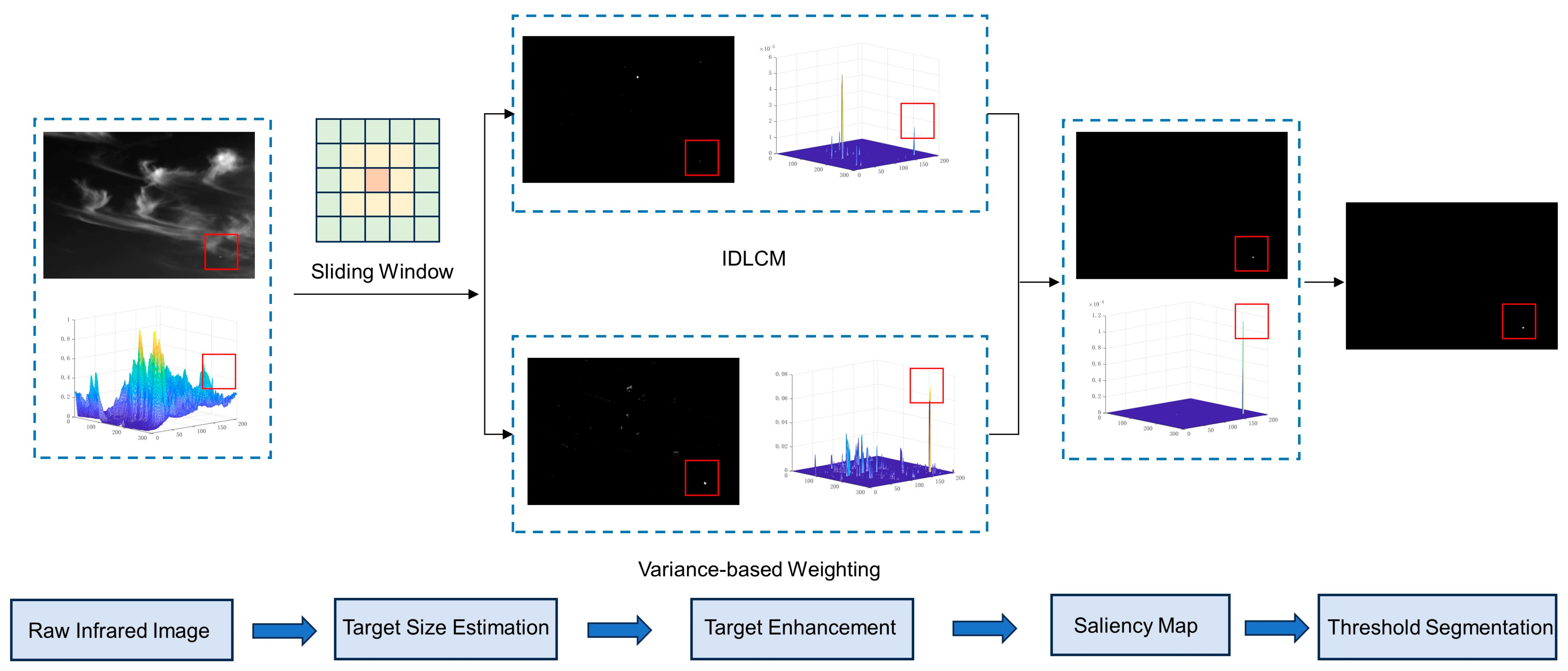
The rest of this paper is organized as follows. In Section 2, we introduce the proposed WIDLCM in detail. Extensive experimental results and comparisons with several other state-of-the-art methods are presented in Section 3. In Section 4, we demonstrate ablation experiments to validate the necessity of each part of the algorithm and demonstrate the robustness of our algorithm through validation experiments. The conclusion is presented in Section 5.

2. Proposed Method

The flowchart of the WIDLCM algorithm proposed is shown in Figure 1. The algorithm consists of two main steps, target size estimation and target enhancement. We used a fixed-scale three-layer sliding window to screen candidate target pixels and estimate target size according to the comparison of the double neighborhood gray difference. The target enhancement module included an improved double local contrast measure and a variance-based weighting coefficient. The design of the former was based on the difference between the gray values of the target and the background, while the latter was based on the structural difference between them. Clutter was suppressed in the saliency map obtained by target enhancement, and the target was segmented by a simple adaptive threshold.

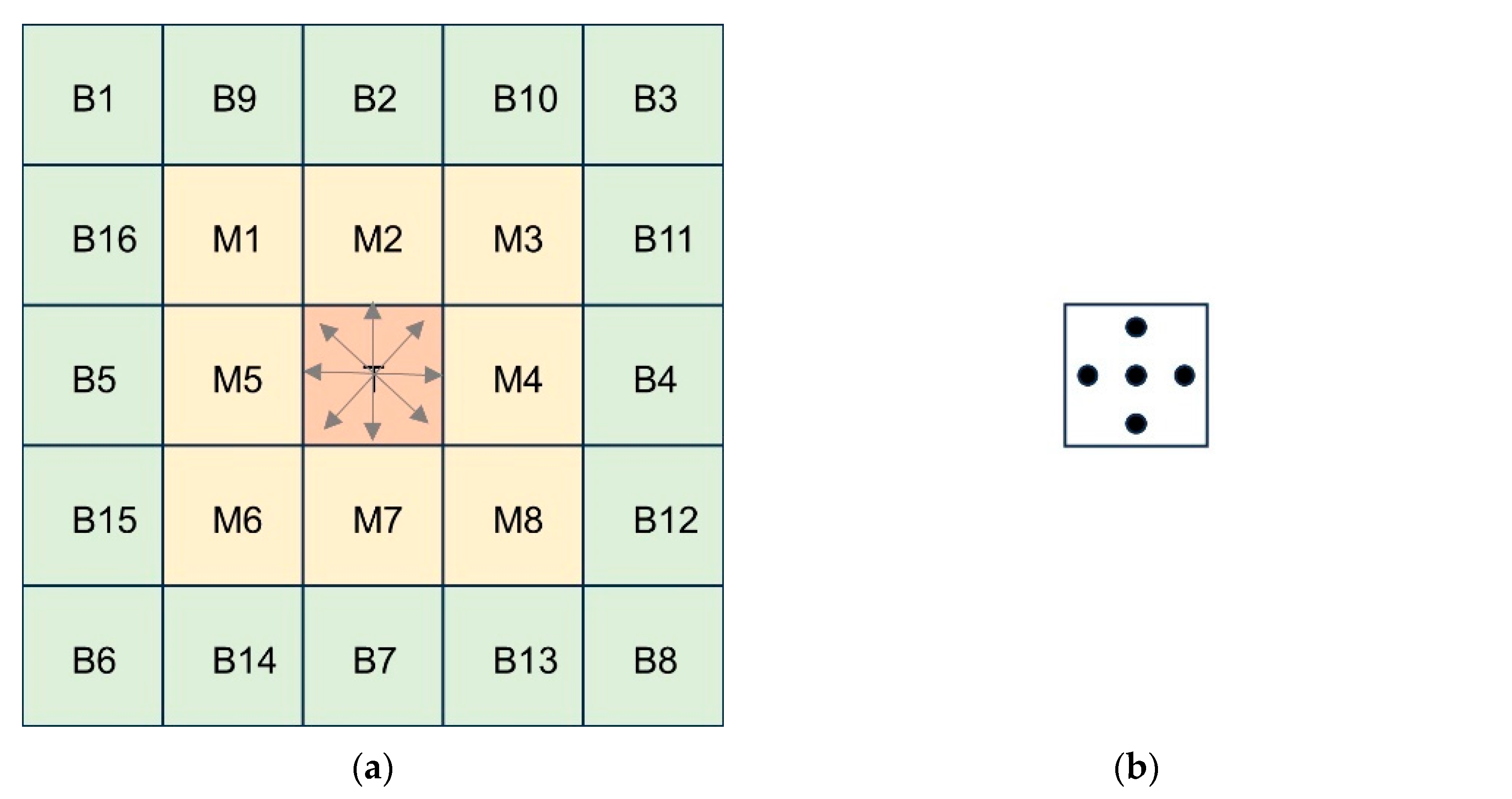
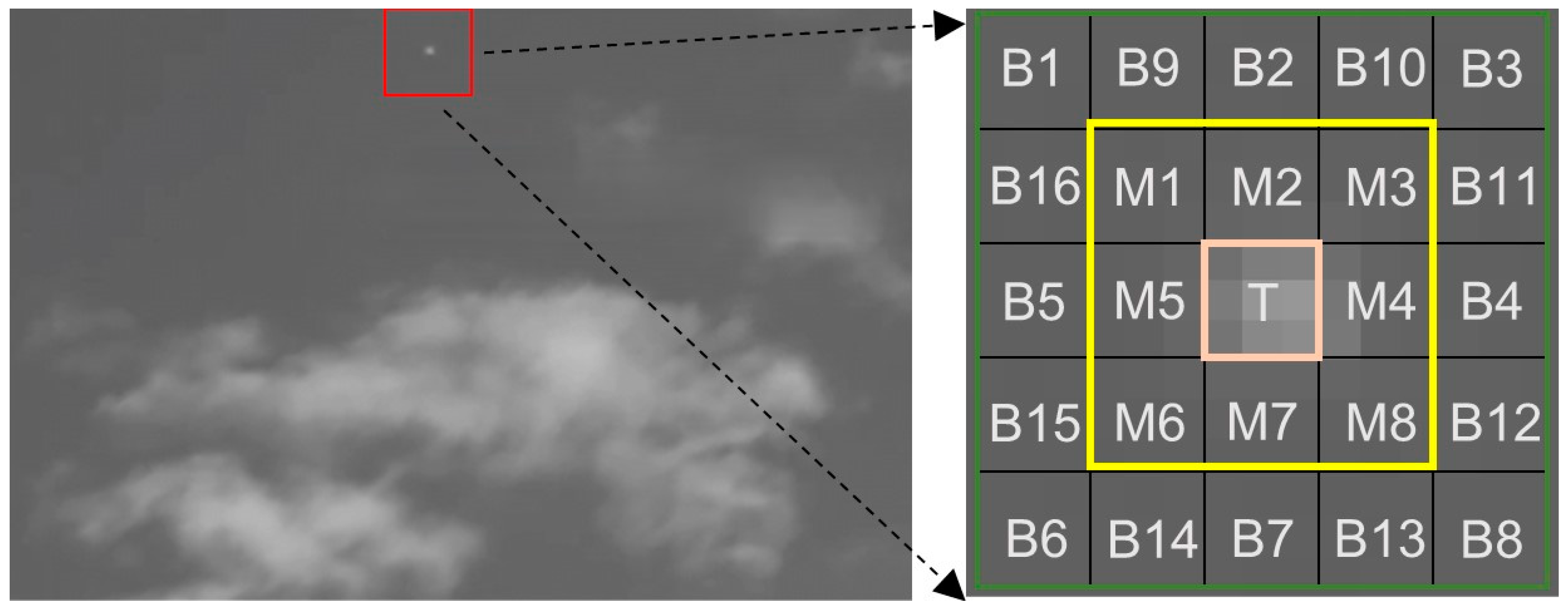
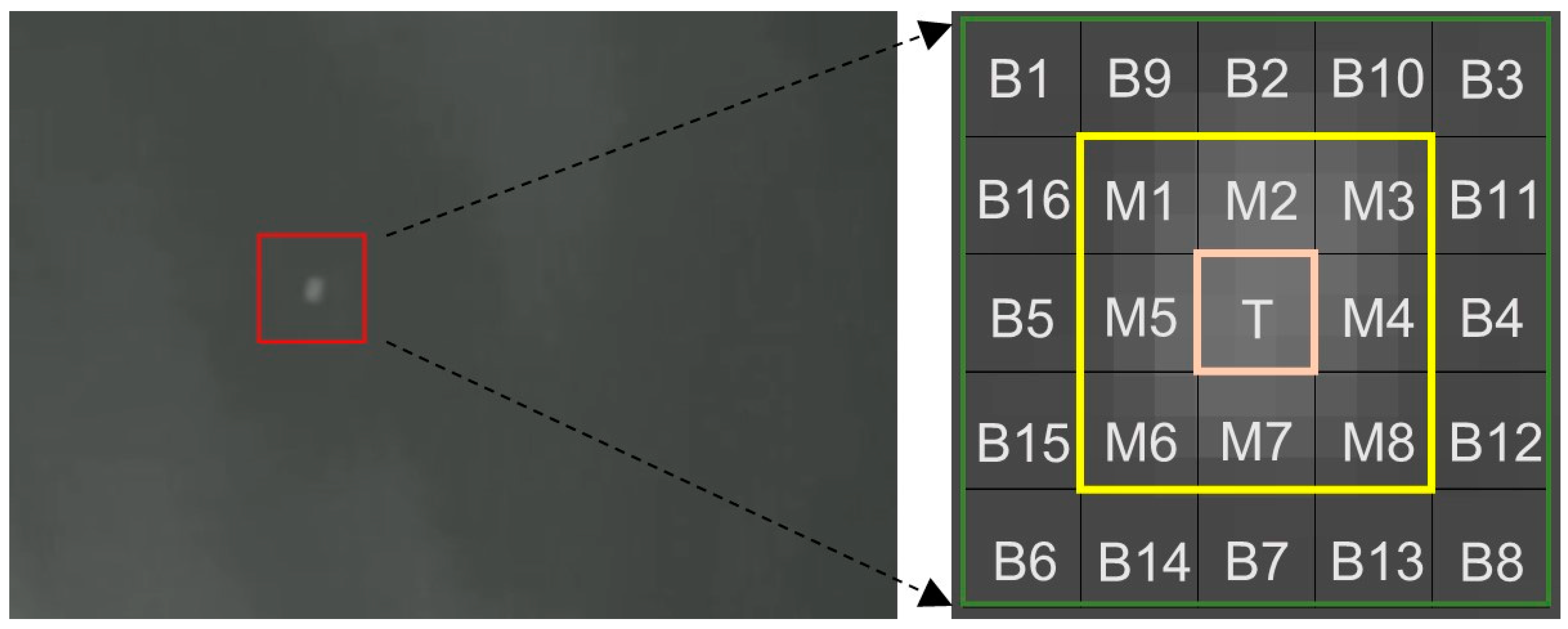
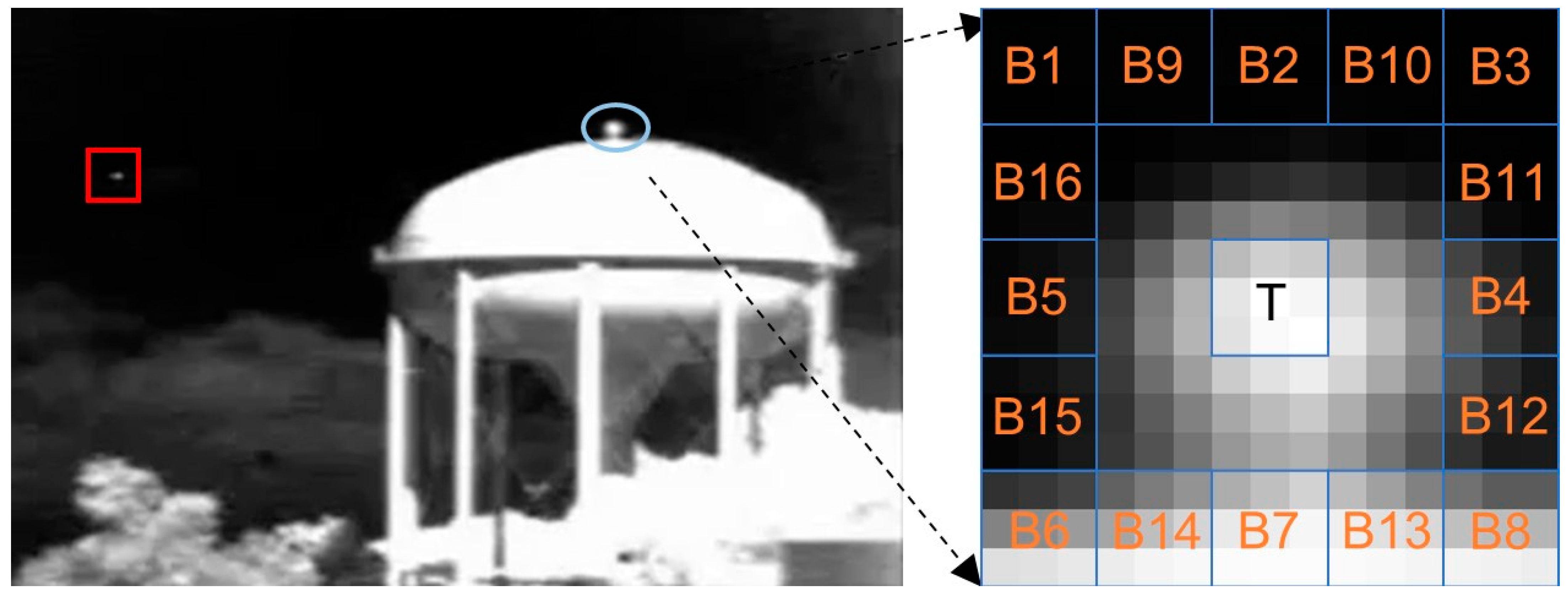
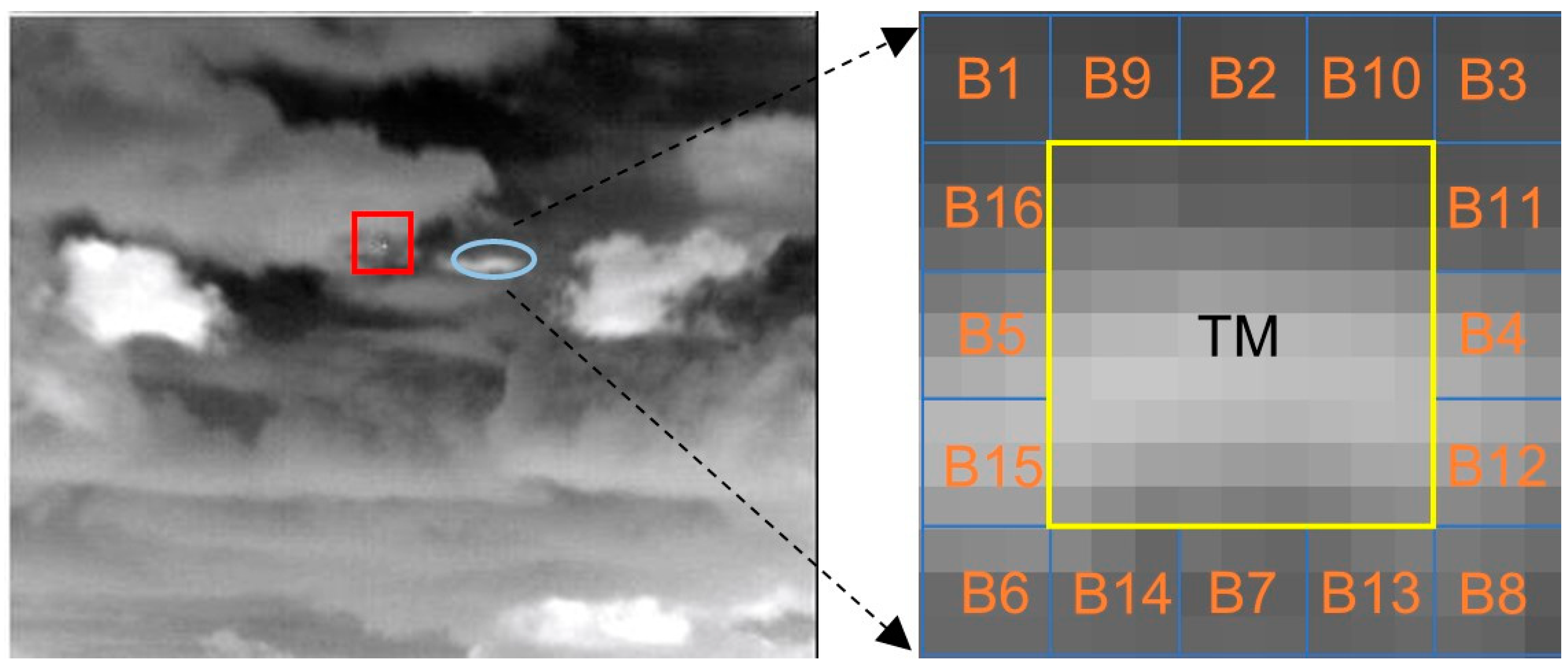
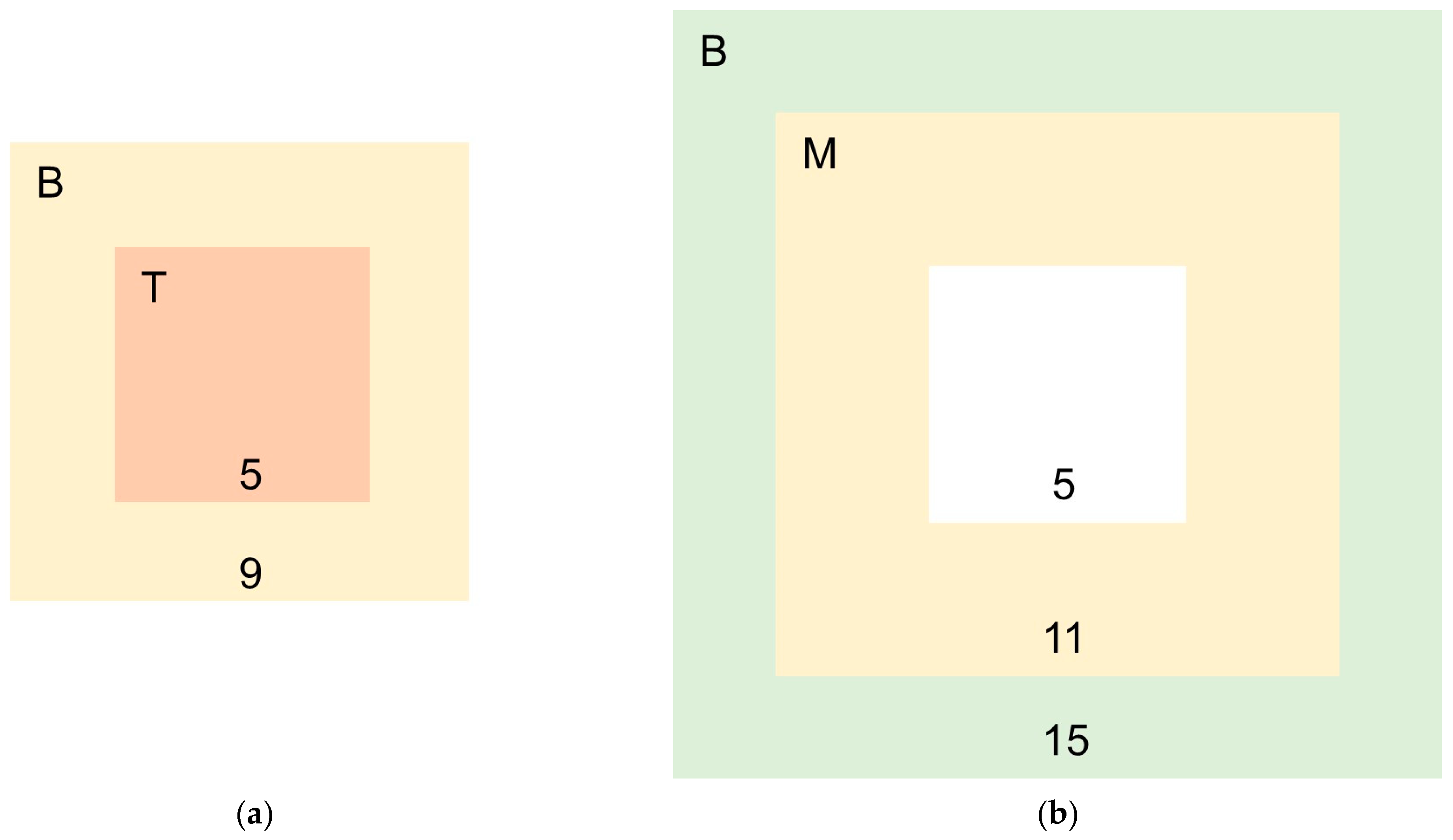
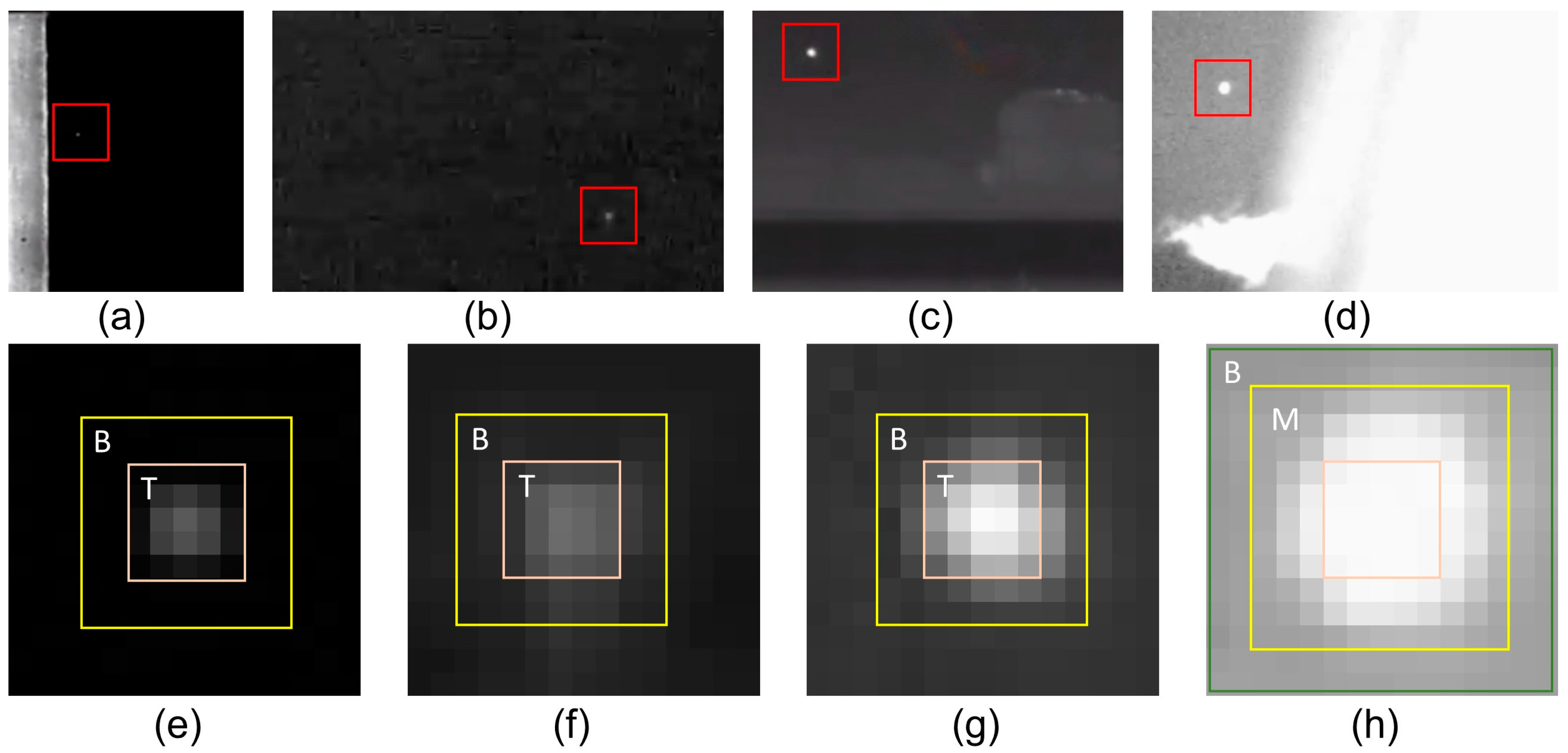
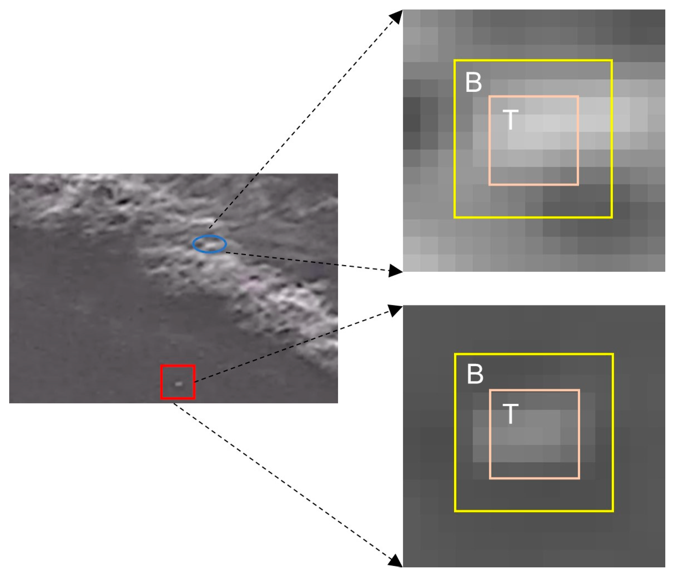
2.1. Candidate Target Pixels’ Screening and Size Estimation

A small target is usually defined to have a total spatial extent of less than 80 pixels [17], ranging from 2 × 2 to about 9 × 9 pixels [37]. The early local contrast methods [17,18,31] use a two-layer window to calculate the contrast measure of the gray difference between the central cell and background cells in the neighborhood and determine the target size by a multi-scale operation. A multi-scale operation is often time consuming, and to avoid this problem, many researchers adopted a fixed-scale three-layer window [19,20,26]. But they did not further consider the size of the target. We used a similar fixed-scale three-layer window and further divided the small target into larger or smaller targets through a simple gray difference comparison method.

The three-layer sliding window we used is shown in Figure 2a. The central layer, middle layer, and outermost layer were composed of 1, 8, and 16 cells with a size of 3 × 3 pixels, respectively. The central cell captured the central part of the target that may be present in the current location. The eight cells in the middle layer may be the edge of the target or the adjacent background of the target due to the different sizes of the target. The sixteen outermost cells describe the background properties around the target. Most studies used all pixels in a cell for gray difference measure calculation. We only used five pixels instead of all pixels to measure the gray characteristics of the cell, as shown in Figure 2b, to prevent small targets with a size of approximately 2 × 2 from being weakened.

Previously, the multi-scale technique typically used four scales (i.e., 3, 5, 7, 9) to represent the target size. We divided the first two scales into smaller targets and the last two scales into larger targets. Based on the assumption that the target was isotropic and there was usually a significant difference in the gray value between the target edge and the background, we determined the candidate target pixels and whether the target was a larger target or a smaller target by the double neighborhood gray difference in eight directions.

We first calculated the double neighborhood gray difference in eight directions, defined as follows.

$$\left\{\begin{array}{c}d{TM}_i=mT-m{M}_i,(i=1,\dots \dots ,8)\\ d{MB}_j=m{M}_j-m{B}_j,(j=1,\dots \dots ,8)\end{array}\right. ,$$

(1)

where $mT$, $m{M}_i$, $m{M}_j$, $and m{B}_j$ are the average of the gray values of the five pixels of the central cell, the $i$th middle layer cell, the $j$th middle layer cell, and the $j$th outermost layer cell; $d{TM}_i$ represents the difference between the average gray value of the central cell and the average gray value of the $i$th middle layer cell; $d{MB}_j$ represents the difference between the average gray value of the $j$th middle layer cell and the $j$th outermost layer cell. Then we calculated the minimum values of $d{TM}_i$ and $d{MB}_j$ and judged the target size by comparing them.

For each pixel in the image, if $min$($d{TM}_i$) > $min$($d{MB}_j$) and $min$($d{TM}_i$) > 0, the pixel was a candidate for smaller targets. For smaller targets, this judgement condition was clearly true, as shown in Figure 3. If $min$($d{MB}_j$) > $min$($d{TM}_i$) and $min$($d{MB}_j$) > 0, the pixel was a candidate for larger targets. If neither condition was met, it was not a candidate target pixel. For larger targets, the gray value change from the center to the edge of the target may be smaller than the gray difference between the target edge and background, as shown in Figure 4. Therefore, we calculated the difference in gray values between the middle layer cells and the outermost layer cells as a judgment.

2.2. Calculation of IDLCM

Based on the size information of the potential target pixels and the gray difference in the adjacent cells in eight directions obtained in Section 2.1, we defined the first local contrast measure similar to [19], which used the product of the gray difference in the diagonal direction for target enhancement.

For smaller target candidate pixels, the first local contrast measure was calculated using the following equation:

$${LCM}_1=\underset{i=\mathrm{1,2},\mathrm{3,4}}{\min }(d{TM}_i\times d{TM}_{9-i}),$$

(2)

For larger target candidate pixels, the first local contrast measure was defined as follows:

$${LCM}_1=\underset{j=\mathrm{1,2},\mathrm{3,4}}{\min }(d{MB}_j\times d{MB}_{9-j}),$$

(3)

The first local contrast measure of IDLCM only utilized the gray values of the adjacent two layers, while in the second local contrast measure, the gray values of the other layer in the three-layer window were used to further eliminate interference.

For smaller target candidate pixels, the second local contrast measure was calculated using the following equation:

$${\mathit{LCM}}_2=\underset{j=1,\dots \dots ,16}{\min }\left(\left|mT-m{B}_j\right|\right),$$

(4)

The definitions of $mT$ and $m{B}_j$ are consistent with those in Section 2.1. We used the absolute value of the gray difference between the central cell and the outermost background cell to avoid missing detection when the target was close to the high-brightness background. In addition, it can also eliminate some clutter interference. As shown in Figure 5, during the first local contrast measure calculation process, the top of the building was mistakenly identified as a smaller target. After the first enhancement, it was much brighter than the real target. However, through the second local contrast measure calculation, the similarity of the gray values between the outermost and central cells was taken into account, resulting in a significant reduction in brightness at the top of the building and effective enhancement of the real target.

For larger target candidate pixels, the second local contrast measure was calculated using the following equation:

$${LCM}_2=\left\{\begin{array}{c}\underset{j=1,\dots \dots ,16}{\min }\left(mTM-m{B}_j\right), if\underset{j=1,\dots \dots ,16}{\min }\left(mTM-m{B}_j\right)>0\\ 0, else\end{array}\right. ,$$

(5)

The definition of $m{B}_j$ is the same as in Section 2.1. The $mTM$ is the average gray value of all pixels (i.e., 81 pixels) in the central cell and middle layer. In the process of determining candidate pixels for larger targets in Section 2.1, we did not consider the gray values of the central cells. For real larger targets, the average gray value of the central cell and the middle layer should be greater than the outermost layer. As shown in Figure 6, the cloud edge was mistakenly identified as a larger target, and after calculating the second local contrast measure, it was successfully eliminated.

For larger and smaller target candidate pixels, by combining their respective ${LCM}_1$ and ${LCM}_2$, the improved double local contrast measure (IDLCM) was defined as follows:

$$IDLCM={{LCM}_1\times LCM}_2,$$

(6)

2.3. Calculation of Variance-Based Weighting Coefficient

The definition of IDLCM takes full advantage of the gray value difference between the target and background, but interferences in the background may also have this characteristic. In general, the target edge is closed and circular. The gray values change significantly at the edge, and the adjacent background is relatively uniform. However, interference, such as buildings, is usually large and continuous. Even if there are gray differences similar to the target in some areas, the adjacent regions are not entirely the background, resulting in notable gray value variations. Variance can be used to describe the distribution of gray values. Thus, we proposed the variance-based weighting coefficient to further eliminate clutter.

Mu et al. [25] proposed a variance difference measure that assumes that the variance of the central and middle layers is greater than the variance of the outermost layer when the target is present. However, this variance difference measure cannot effectively suppress clutter, and its enhancement effect on smaller targets is poor. Figure 7a shows an infrared image containing a 2 × 2-sized target, and Figure 7b shows the corresponding variance difference measure. Due to the small size of the target and its proximity to high-brightness interference, the variance difference measure at the target position was less than 0, resulting in the missed detection of the target.

According to the target size estimation steps in Section 2.1, we could roughly determine the edge position. Then, we designed two new windows for smaller and larger targets to calculate weighting coefficients, as shown in Figure 8a,b.

For smaller target candidate pixels, using the two-layer window in Figure 8a, the inner window size is 5 pixels, the outer window size is 9 pixels, and the variance-based weighting coefficient is defined as follows:

$$WV=V_T-V_B,$$

(7)

$V_T$ and $V_B$ are the variances of the gray values of all pixels in the inner and outer layers, respectively.

For larger target candidate pixels, using the window in Figure 8b, the inner window size is 5 pixels, the middle window size is 11 pixels, and the outermost window size is 15 pixels. The weighting coefficient is defined as follows:

$$WV=V_M-V_B,$$

(8)

$V_M$ and $V_B$ are the variances of the gray values of all pixels in the middle and outermost layers, respectively. We did not consider the pixels in the central layer because, according to our previous judgment of larger targets, the gray values from the central layer to the middle layer of the target did not change much, as shown in Figure 9h. In the weighting coefficient calculation window designed for larger targets, the gray values of the target in the central layer and the background in the outermost layer were relatively uniform, and the edge of the target with changes in gray values was located in the middle layer. Therefore, $V_M$ > $V_B$, $WV$ > 0.

Figure 9 shows the weighting coefficient calculation windows for targets of different sizes. Figure 9e,f show the windows for targets with sizes of 3 × 3 (Figure 9a) and 5 × 5 (Figure 9b), respectively. For smaller targets, it can be seen that the gray value of the target changed mainly in the inner window, while the background around the target in the outer window was relatively uniform. Therefore, $V_T$ > $V_B$, $WV$ > 0.

Figure 9g shows the calculation window for the 7 × 7-sized target in Figure 9c. In the process of target size estimation, the gray value change in the target from the central cell to the middle layer was greater than the change from the middle layer to the outermost layer, so it was judged as a smaller target rather than a larger one. In this case, the weighting coefficient calculation window designed for smaller targets also performed well. Figure 9h shows the calculation window for the 9 × 9-sized target in Figure 9d. The large area of high-brightness interference on the right side in Figure 9d can be easily suppressed by our gray difference measure. The weighting coefficient can further suppress the interference of these fragmented bright cloud edges, as their continuity leads to close variances between the two layers in the weighting coefficient calculation window.

Figure 10 shows the clutter suppression effect of the weighting coefficient we designed. There were many interferences in the background that were similar to the target, and their gray values were higher than the surrounding background. Therefore, it was difficult to suppress clutter by the gray value difference measure. However, the background around a target is usually homogeneous, while the background of clutter varies greatly. As shown in Figure 10, for the target, $V_T>V_B$, $WV>0$, and for clutter, $V_T\approx V_B$, $WV\approx 0$.

2.4. Calculation of WIDLCM

After calculating the improved double local contrast measure and variance-based weighting coefficient, the WIDLCM of a pixel is defined as

$$WIDLCM\left(x,y\right)=\left\{\begin{array}{ll}IDLCM\left(x,y\right)\times WV\left(x,y\right),& for candidate target pixels\\ 0,& else\end{array}\right.$$

(9)

For each pixel, $IDLCM(x,y)$ and $WV(x,y)$ are calculated based on the estimated target size information of that pixel.

2.5. Threshold Operation

In the final WIDLCM saliency map, the target was greatly enhanced and most clutter was eliminated. Therefore, a simple adaptive threshold was used to segment the real target. The threshold was defined as:

$$Th=\mathrm{m}\mathrm{e}\mathrm{a}\mathrm{n}\left(\mathrm{W}\mathrm{I}\mathrm{D}\mathrm{L}\mathrm{C}\mathrm{M}\right)+k\times \mathrm{s}\mathrm{t}\mathrm{d}\left(\mathrm{W}\mathrm{I}\mathrm{D}\mathrm{L}\mathrm{C}\mathrm{M}\right)$$

(10)

where $\mathrm{m}\mathrm{e}\mathrm{a}\mathrm{n}\left(\mathrm{W}\mathrm{I}\mathrm{D}\mathrm{L}\mathrm{C}\mathrm{M}\right)$ and $\mathrm{s}\mathrm{t}\mathrm{d}\left(\mathrm{W}\mathrm{I}\mathrm{D}\mathrm{L}\mathrm{C}\mathrm{M}\right)$ are the mean and standard deviation of the WIDLCM map, respectively, and $k$ is a parameter; our experiments showed that a $k$ between 20 and 60 will be proper. A value of $k$ higher than this range can easily lead to the missed detection of the target, while a value lower than this range can result in more false alarms.

3. Experimental Results

To verify the effectiveness of our proposed method, we chose eight advanced local contrast methods for comparison, including MPCM [18], WSLCM [34], ADMD [38], DLCM [19], DNGM [20], WTLLCM [35], TLLDM [25], and DLPC [26]. Qualitative and quantitative experimental results proved the superiority of our method. All experiments were conducted in MATLAB 2021a on a laptop with 3.2-GHz AMD R7 CPU and 16-GB RAM.

3.1. Datasets

Our experiment used eight real infrared image sequences that are publicly available for small target detection research. Sequence 1, Sequence 2, and Sequence 3 are from [39]. The three sequences cover different backgrounds, with each image containing a bright aircraft target. Sequence 1 contains 396 images, with the main interference in the background being high-brightness ground. Sequence 2 and Sequence 3 consist of 600 and 260 images, respectively. Note that there are many buildings with strong radiation in the background of these two image sequences, which can easily cause false alarms. Sequence 4 is a subset of the SIRST dataset [13]. The SIRST dataset contains 427 images, of which we only used images containing a single target and removed some images with target sizes larger than the defined small targets mentioned earlier. The final Sequence 4 has a total of 279 single-target images, including aircraft, vehicles, ships, and other targets, covering the sky, sea, and ground background. The remaining four sequences are from the IST-A dataset [40]. These four datasets focus on aircraft targets in the sky. Figure 11 shows a typical scene for each image sequence. Detailed information on the eight datasets is presented in

Table 1. Details of the eight test sequences.

Sequence	Frames	Target Type	Target Size	Target Number	Background Description
1	396	aircraft	2 × 2 to 3 × 3	1	Ground background, forests, high-brightness ground
2	600	aircraft	2 × 2 to 4 × 3	1	Ground background, forests, high-brightness buildings, high-voltage towers
3	260	aircraft	3 × 3 to 3 × 4	1	Ground-sky background, forests, high-brightness buildings
4	279	aircraft, vehicle, ship, others	2 × 2 to 9 × 9	1	Various backgrounds, heavy cloud, high-brightness buildings, heavy noise
5	70	aircraft	3 × 3 to 5 × 4	1	Sky background, cloud, high-brightness trees
6	125	aircraft	4 × 4 to 11 × 5	1	Sky background, cloud, high-brightness trees, buildings
7	60	aircraft	4 × 4 to 5 × 4	1	Sky background, cloud, high-brightness buildings
8	55	aircraft	4 × 3 to 7 × 6	1	Sky background, cloud, high-brightness trees

.

3.2. Evaluation Metrics

We quantitatively compared the performance of each algorithm using four commonly used evaluation metrics: signal-to-clutter ratio gain (SCRG), background suppression factor (BSF), receiver operating characteristic curve (ROC), and consumption time.

The SCRG and BSF characterize the ability of the algorithm to enhance the target and suppress the background; we used the definitions in [41] and made some improvements.

The SCRG in this paper is defined as follows:

$$SCRG={\displaystyle \frac{{SCR}_{out}}{{SCR}_{in}}},{SCR}_{in}={\displaystyle \frac{|{\mu }_t-{\mu }_b|}{{\sigma }_b}},{SCR}_{out}={\displaystyle \frac{|{\mu }_t-{\mu }_b|}{{\sigma }_b+\epsilon }}$$

(11)

where ${\mu }_t$ is the average gray value of the target, ${\mu }_b$ is the average gray value of the background surrounding the target, and ${\sigma }_b$ is the standard deviation of the background surrounding the target. ${SCR}_{in}$ and ${SCR}_{out}$ are the signal-to-clutter ratios of the original infrared image and the saliency map after being processed by the algorithm, respectively. In general, ${\sigma }_b$ of the original image is unlikely to be 0, but ${\sigma }_b$ of the saliency map may be 0. To avoid infinity (Inf), we added a small constant $\epsilon$ to the denominator of the signal-to-clutter ratio calculation formula of the saliency map. The value of $\epsilon$ in the experiment was set as 0.0001.

The BSF is defined as

$$BSF={\displaystyle \frac{{\delta }_{in}}{{\delta }_{out}+\epsilon }}$$

(12)

where ${\delta }_{in}$ and ${\delta }_{out}$ are the standard deviations of the background in the original infrared image and the saliency map, respectively. We also added the same constant $\epsilon$ to the denominator to prevent the result from being infinity (Inf).

The larger the values of BSF and SCRG, the stronger the algorithm’s ability to enhance the target and eliminate background clutter was.

The ROC curve can show the detection ability of the algorithm more intuitively. The true-positive rate (TPR) and the false-positive rate (FPR) are two key parameters for plotting the ROC curve. TPR and FPR represent the detection probability $P_d$ and false-alarm rate $F_a$, respectively, which are defined as follows:

$$P_d={\displaystyle \frac{number of true targets detected}{total number of true targets}}$$

(13)

$$F_a={\displaystyle \frac{number of false detected pixels}{total number of pixels in the whole image}}$$

(14)

The ROC curve is plotted with a false-alarm rate as the horizontal axis and a detection probability as the vertical axis. The closer the curve is to the upper left corner, the stronger the detection ability of the algorithm is.

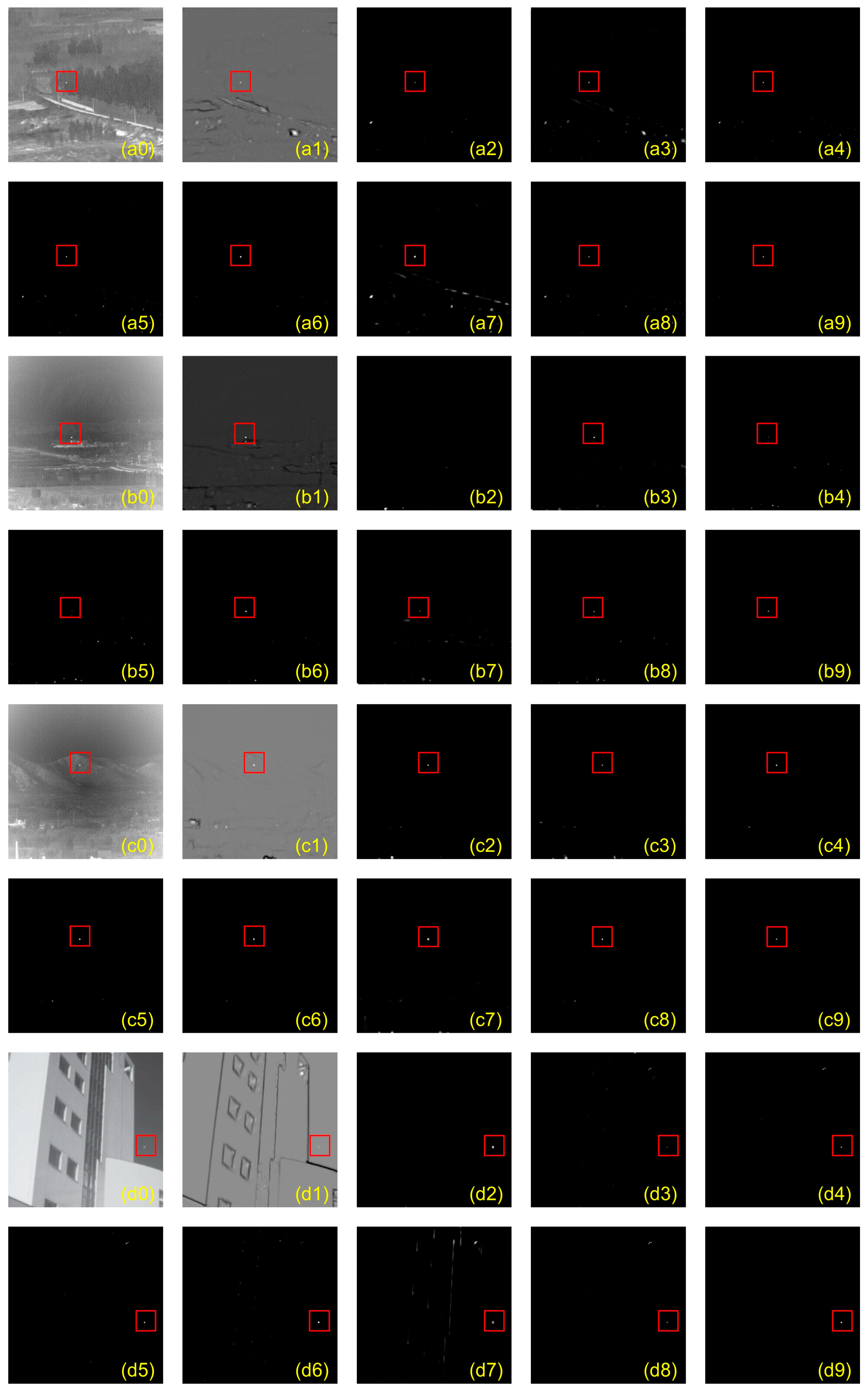
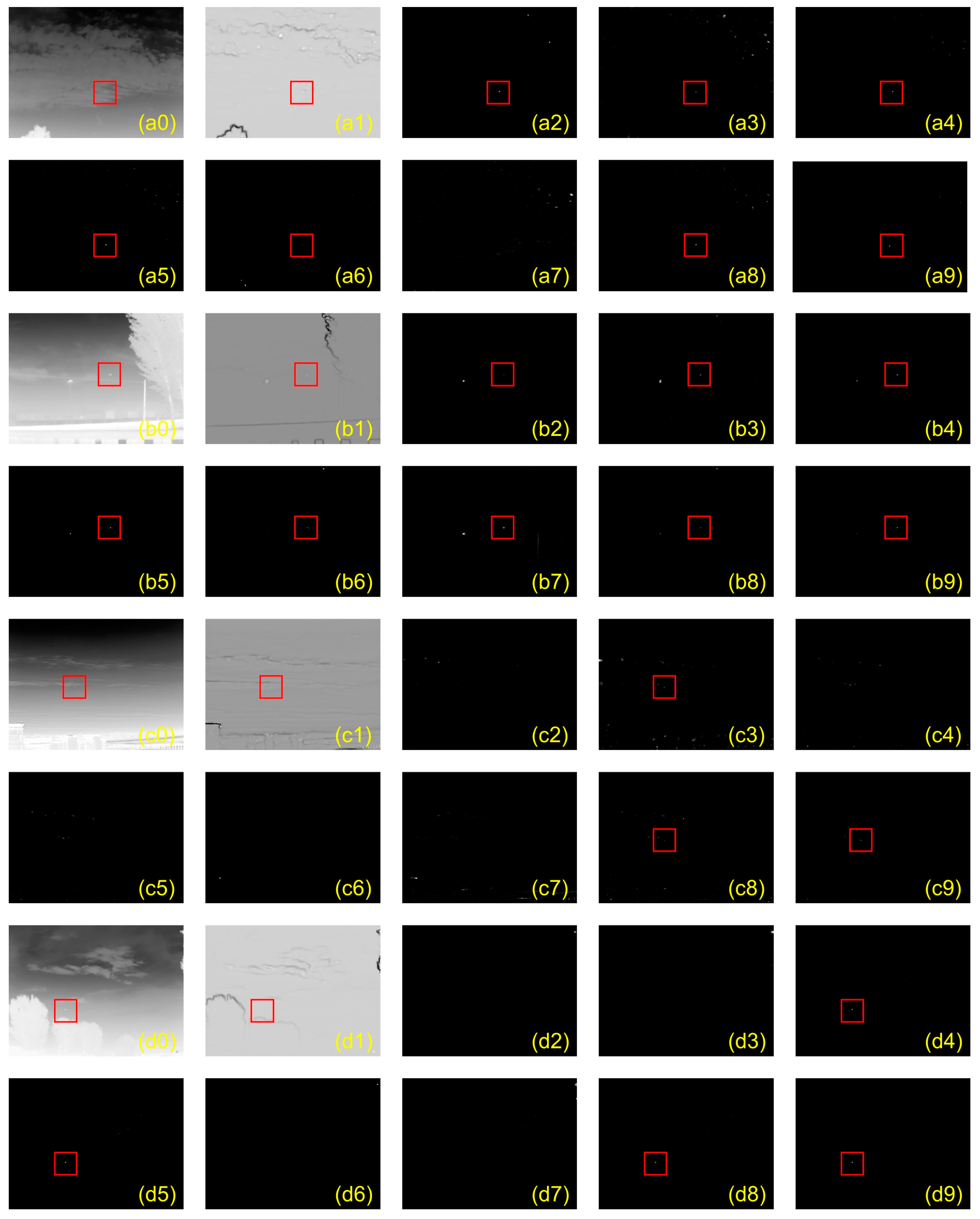
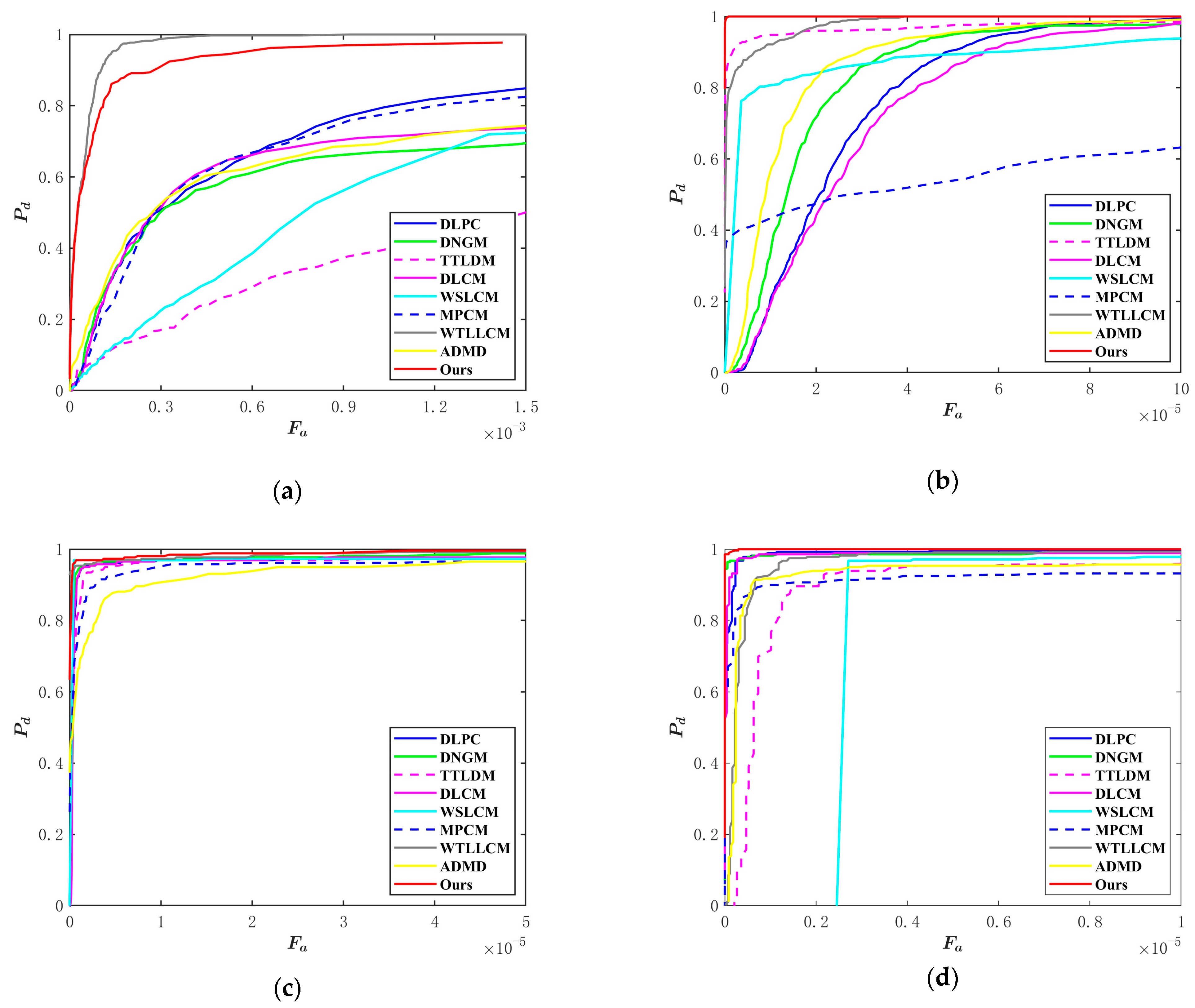
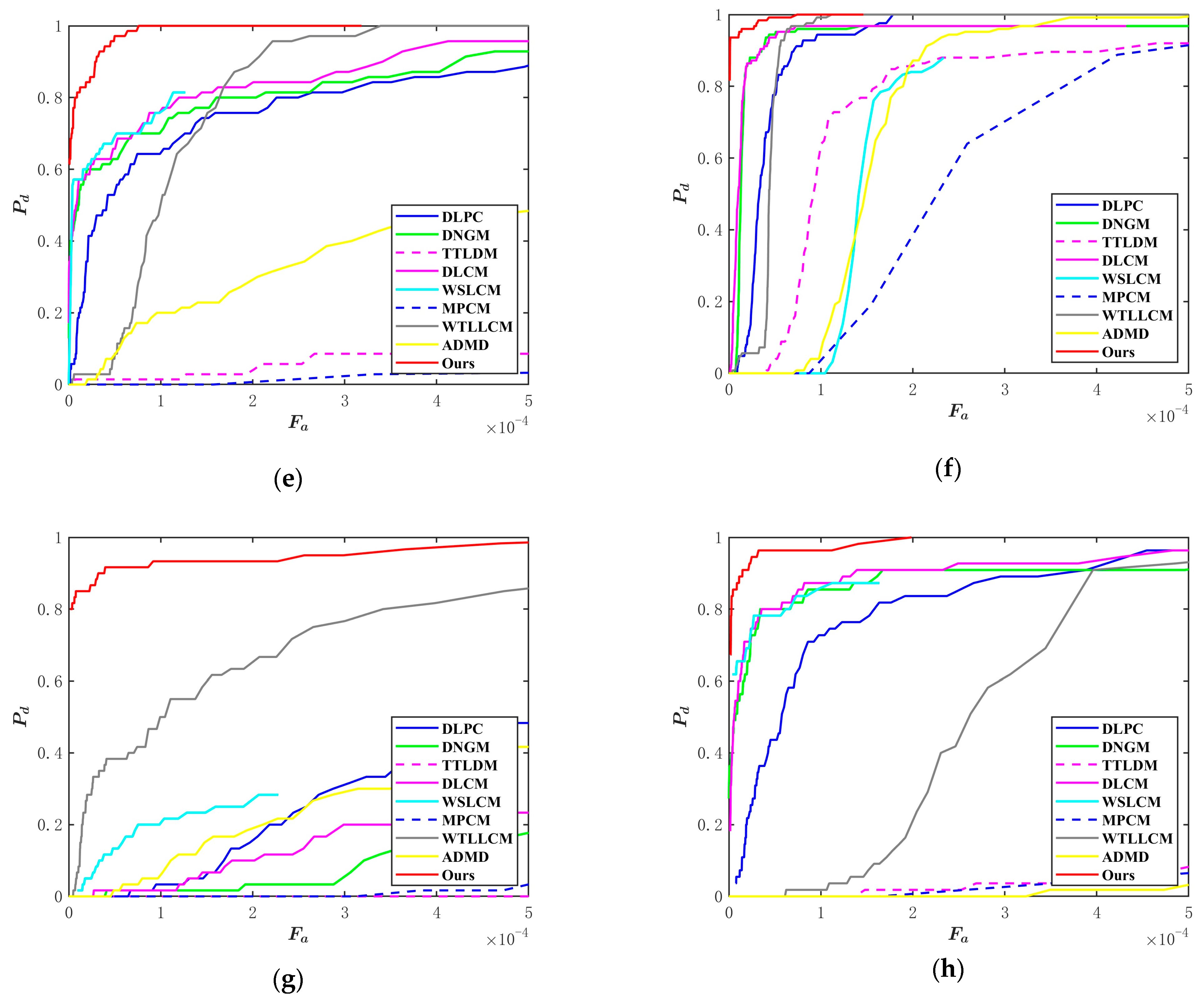
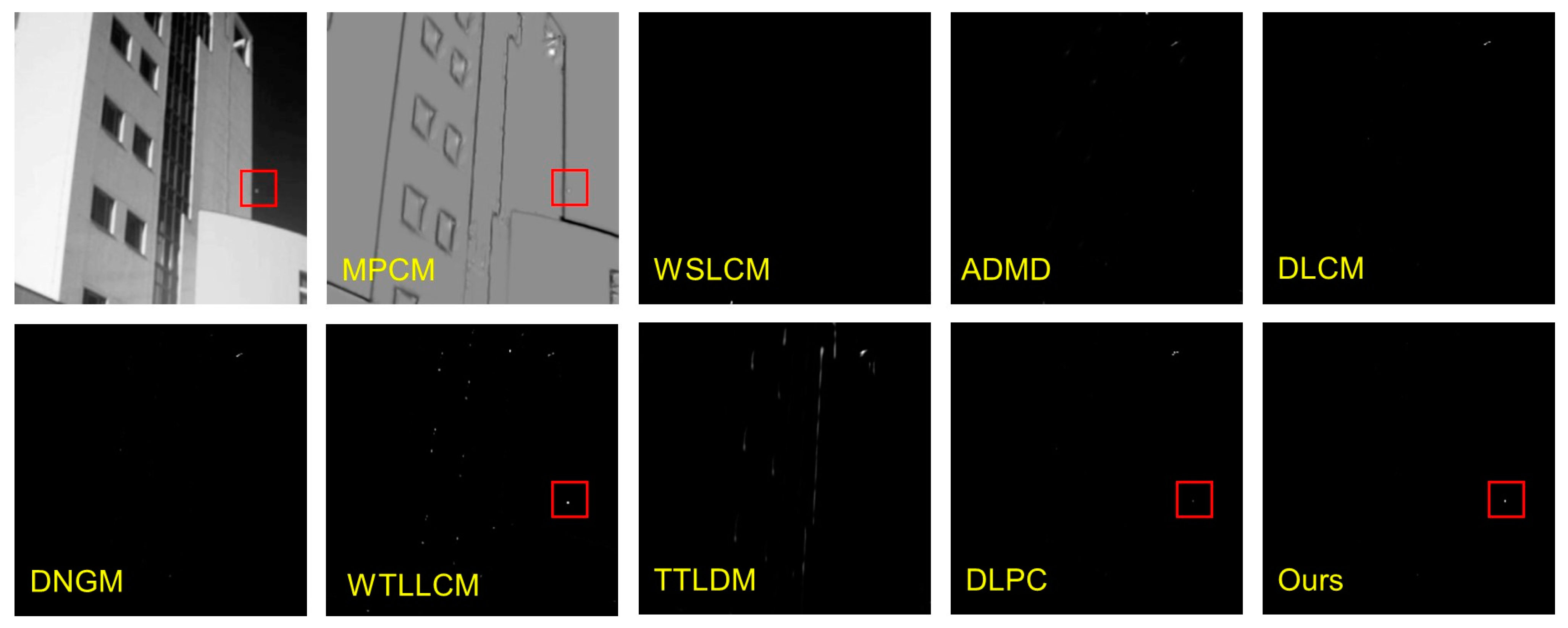
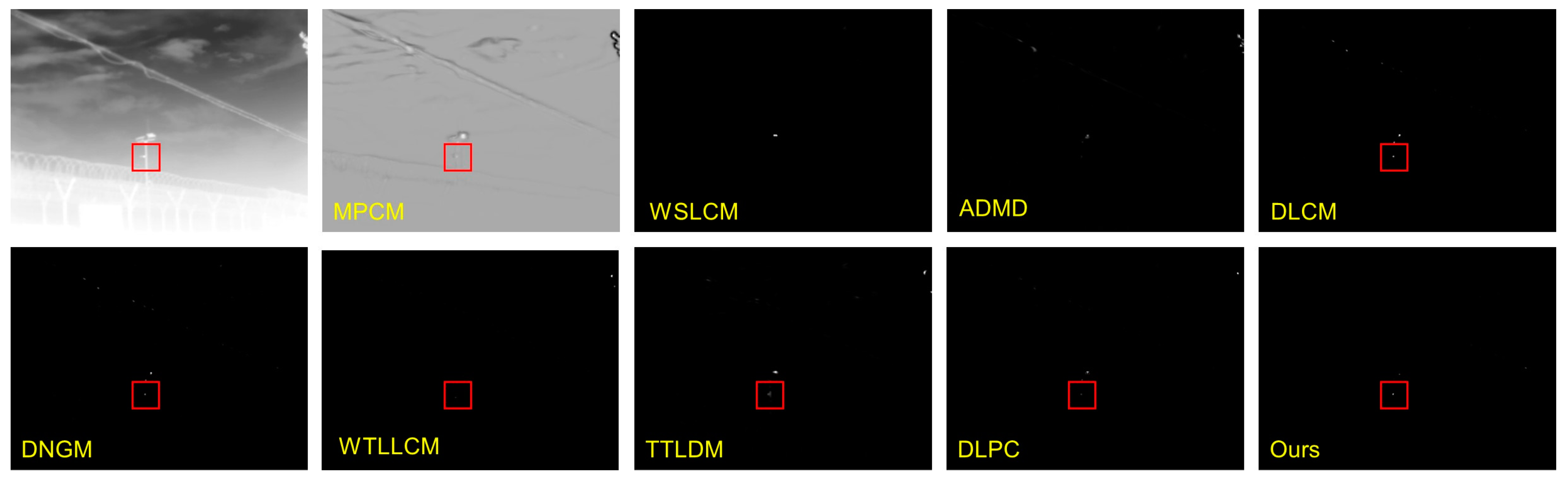
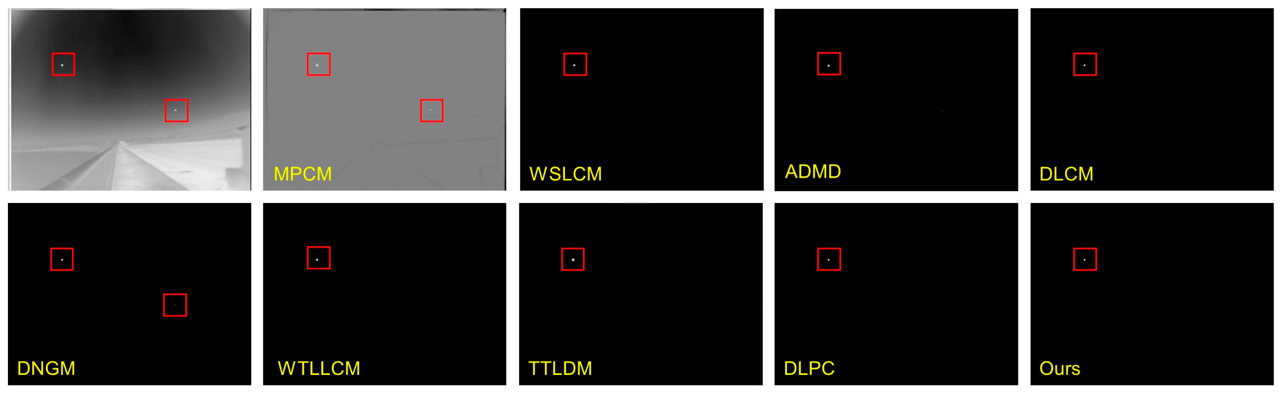
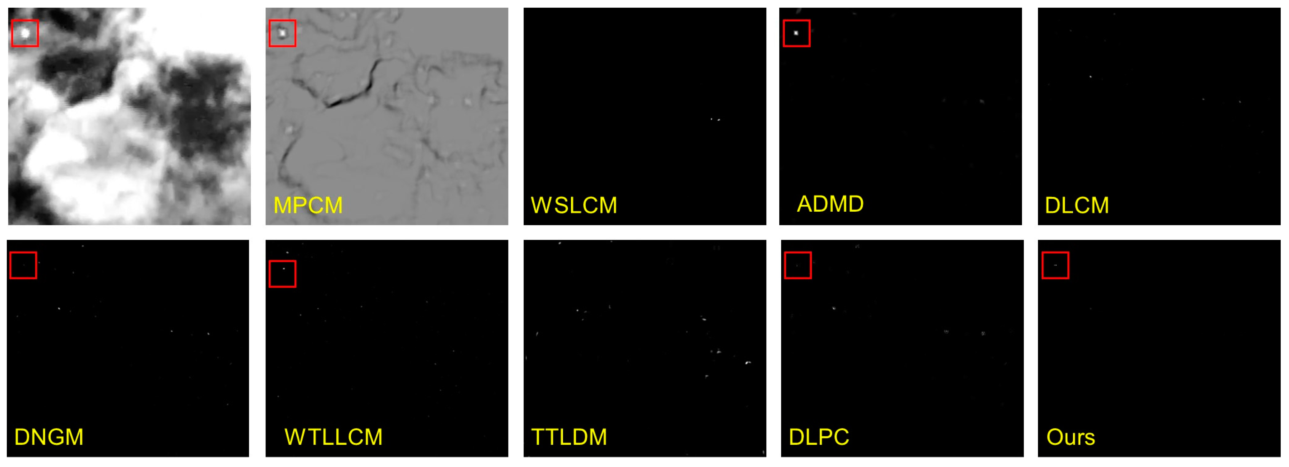
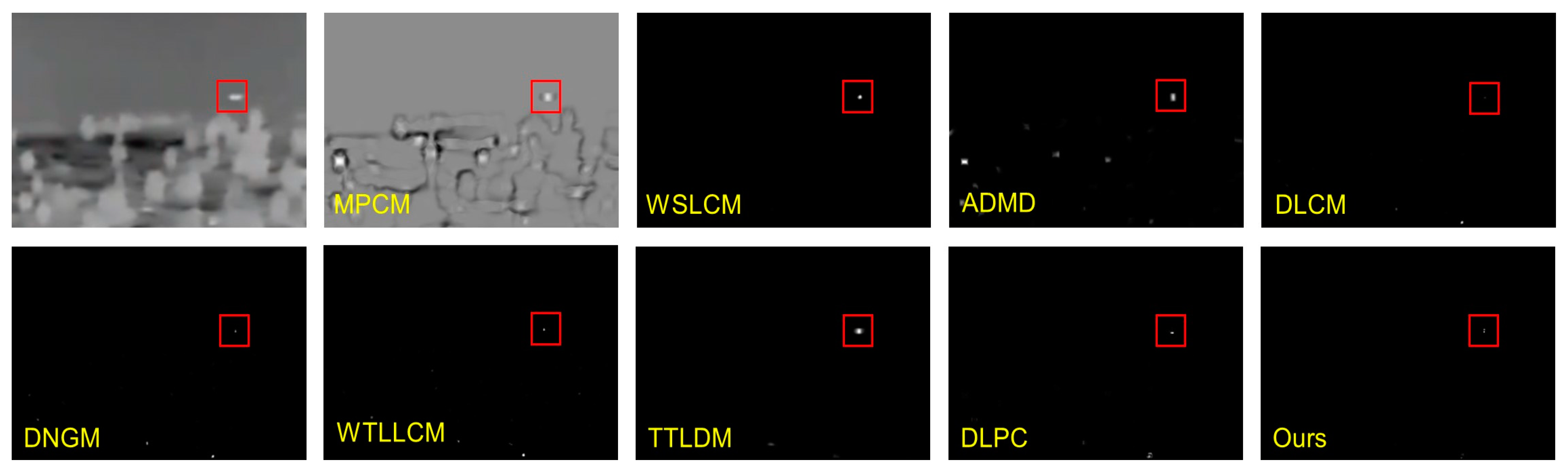
3.3. Qualitative and Quantitative Comparison Results

For this section, we qualitatively and quantitatively compared our algorithm with eight other state-of-the-art algorithms on the eight datasets.

Figure 12 and Figure 13 show the detection results of different algorithms on sample images from the eight datasets. The target is marked with a red rectangular box, and the unmarked rectangular box represents the missed target. In Sequence 1, except for our method and WTLLCM, all other methods erroneously enhanced the high-brightness ground interference, causing its brightness to be close to or even higher than the real target. In the sample image of Sequence 2, the target was adjacent to high-brightness interference. WSLCM missed the real target. DLCM, DNGM, and TLLDM had weak enhancement effects on the target. Compared with the remaining four methods, our method was more effective in suppressing the background. In Sequence 3, all methods successfully enhanced the target, but the other eight methods still had residual clutter. In Sequence 4, compared to the other seven algorithms, WSLCM and our method could eliminate interference from the high-brightness building in the background. In Sequence 5, the target was submerged in bright clouds. The fragmented bright clouds caused a lot of interference, which can be seen in the results of MPCM, WSLCM, ADMD, and TTLDM. And WTLLCM erroneously enhanced the tree in the bottom left corner. In Sequences 6, 7, and 8, there was high-brightness interference from buildings and trees in the background. Only our method enhanced the target while eliminating these interferences.

Among the methods mentioned above, MPCM, ADMD, DLCM, DNGM, and DLPC only considered the gray difference between the target and background, making it easy to enhance high-brightness background interference. TTLDM designed a rough variance difference measure that can easily enhance clutter. WSLCM designed a sophisticated weighting function that can effectively suppress clutter in certain situations. WTLLCM used a 5 × 5 layered gradient kernel for filtering and performed local contrast calculation on the filtered image. Without using the information from the original infrared image, it was easy to mistakenly identify the high-brightness areas of buildings and trees as targets. Our method considered the size of the target and designed the corresponding gray difference measure and weighting coefficient, achieving better target detection performance.

The quantitative experimental results also demonstrated the superiority of the proposed algorithm.

Table 2. Average BSF of different algorithms.

Sequence	MPCM	WSLCM	ADMD	DLCM	DNGM	WTLLCM	TTLDM	DLPC	Ours
1	5.092	11.534	6.697	13.964	11.389	17.318	6.374	13.146	28.064
2	8.527	45.144	15.619	27.025	22.404	39.710	18.488	26.686	133.774
3	18.936	71.731	22.410	81.677	49.188	62.628	24.035	79.157	264.270
4	64.801	649.941	108.470	1025.176	583.508	888.913	219.631	585.364	1295.452
5	6.924	188.473	16.147	43.573	33.999	35.790	19.783	36.764	186.746
6	11.562	38.832	29.420	60.389	59.629	46.942	29.638	54.500	198.082
7	16.597	49.607	26.668	50.195	36.296	64.373	19.713	45.090	259.731
8	10.379	287.512	25.399	89.992	50.595	48.914	31.947	86.308	455.925

and

Table 3. Average SCRG of different algorithms.

Sequence	MPCM	WSLCM	ADMD	DLCM	DNGM	WTLLCM	TTLDM	DLPC	Ours
1	2.603	21.412	5.772	22.178	14.105	93.389	3.381	11.613	96.219
2	5.030	26.757	9.727	88.520	68.345	96.105	5.214	43.879	139.744
3	5.172	8.712	7.434	84.331	61.507	112.061	2.851	22.194	74.232
4	11.854	202.296	25.688	197.243	157.745	288.923	23.279	82.363	209.836
5	6.443	948.813	257.987	812.916	788.141	371.758	12.754	356.311	1532.261
6	5.395	178.174	74.126	415.472	307.996	207.333	154.366	204.305	490.933
7	36.234	8470.301	3795.154	896.055	1037.347	17,459.412	255.534	2636.521	12,815.916
8	5.039	1516.150	288.563	817.380	892.670	94.176	50.259	362.949	1218.086

show the average BSF and SCRG of each algorithm for the eight datasets. For most sequences, our algorithm obtained the highest BSF value and SCRG value, which indicated that our algorithm has strong background suppression and target enhancement capabilities. WTLLCM achieved good SCRG values on Sequence 1–Sequence 4, but lower BSF values. MPCM, ADMD, and TTLDM showed poor results. Among them, MPCM and ADMD both used multi-scale operation and gray difference contrast to enhance the target, making it easy to enhance clutter with similar gray characteristics. The variance contrast calculation in TTLDM uses a fixed-scale three-layer window, which was difficult to adapt to targets of different sizes.

The ROC curves of different algorithms on the eight test datasets are shown in Figure 14. In Sequence 1, the target was small and there were many small pieces of high-brightness ground in the background causing interference. WTLLCM exhibited better performance than our algorithm because it used a 5 × 5 layered gradient kernel filter, which enhanced smaller targets hidden in clutter better than directly using the average gray difference between the target and the surrounding background. The variance difference measure design of TTLDM lacked consideration for small targets, resulting in poor performance. In Sequence 2, there was high-brightness building interference in the background, which is usually a continuous large area. TTLDM can suppress this kind of clutter, thus achieving better detection performance. In Sequence 3, the presence of buildings with similar target sizes and brightness in the background caused false alarms. The performance of different algorithms on this dataset was similar, and our algorithm achieved a slightly higher detection probability at a low false-alarm rate, followed by WTLLCM and DNGM. In Sequence 4, the size of the target ranged from 2 × 2 to 9 × 9. The background interference was complex and diverse, including high-brightness sea clutter, broken bright clouds, cloud cover, and severe noise. Our method still achieved the best detection results despite these challenges. Among the remaining eight algorithms, MPCM, TTLDM, and WSLCM had poor detection performance on this dataset In Sequences 5 and 7, the targets were small and weak, with broken clouds, bright trees, and buildings causing interference. The proposed algorithm was far superior to the other algorithms. In Sequences 6 and 8, as the size of the target increased, our algorithm still performed well.

Table 4. Average consumption time per frame for different algorithms (in seconds).

Sequence	MPCM	WSLCM	ADMD	DLCM	DNGM	WTLLCM	TTLDM	DLPC	Ours
1	0.028	1.858	0.006	0.021	0.015	0.095	0.006	0.019	0.028
2	0.028	1.865	0.006	0.021	0.014	0.093	0.006	0.019	0.028
3	0.028	1.839	0.006	0.021	0.015	0.093	0.007	0.019	0.028
4	0.027	1.373	0.006	0.020	0.014	0.098	0.007	0.018	0.029
5	0.040	2.379	0.007	0.033	0.020	0.160	0.009	0.026	0.046
6	0.041	2.231	0.007	0.033	0.020	0.153	0.009	0.026	0.045
7	0.041	2.554	0.008	0.033	0.020	0.158	0.010	0.026	0.045
8	0.041	2.239	0.008	0.031	0.020	0.154	0.009	0.026	0.046

shows the average consumption time per frame for each algorithm on four test datasets. It can be seen that ADMD had the shortest running time, followed by TTLDM. WSLCM ran the slowest due to its multi-scale operation and complex weighting function calculation. WTLLCM consumed more than three times the time of our algorithm. Overall, our algorithm performed the best, achieving a good balance between computational efficiency and detection accuracy.

4. Ablation and Validation Experiments

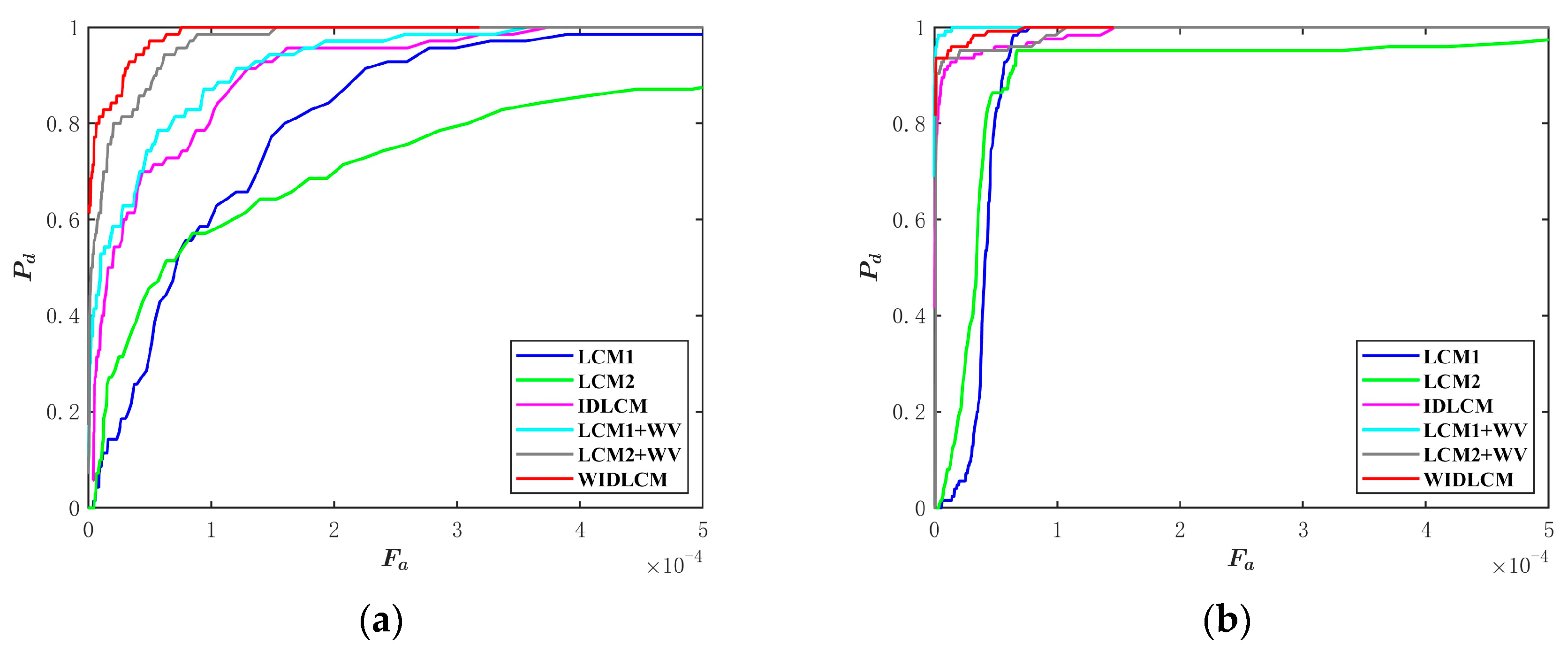
4.1. Ablation Experiments

To demonstrate the effectiveness of each part of the proposed algorithm, we conducted ablation experiments on two datasets with different target sizes (Sequence 5 and Sequence 6). We conducted experiments using LCM1, LCM2, IDLCM, weighted LCM1, weighted LCM2, and WIDLCM, respectively. Figure 15 shows the corresponding ROC curves, while

Table 5. Ablation analysis of our method on Sequence 5 and Sequence 6.

		LCM1	LCM2	IDLCM	LCM1 + WV	LCM2 + WV	WIDLCM
BSF	Seq. 5 Seq. 6	24.377	17.958	53.405	52.998	75.340	186.746
		53.372	32.149	80.076	124.285	82.408	198.082
SCRG	Seq. 5	380.688	486.758	478.025	1424.573	1859.793	1532.261
	Seq. 6	78.363	22.835	302.626	406.900	203.348	490.933

displays the average BSF and SCRG values. It can be seen that each part of the proposed algorithm was effective, especially in the design of the weighting coefficient.

4.2. Validation Experiments

To further validate the robustness of our algorithm, we tested it in three different scenarios. The first scenario was when the target approached the high-brightness edge. As shown in Figure 16, the small dim target was very close to the bright building. WSLCM, ADMD, DLCM, DNGM, and TTLDM missed the target, while MPCM and DLPC did not significantly enhance the target. WTLLCM enhanced both the real target and background interference. Our method successfully detected the target and eliminated high-brightness background interference. The reason is that the second local contrast of the smaller target we designed was not like DNGM, which directly subtracted the gray value of the outermost background from the gray value of the target in the central layer so that the target would not be eliminated. Our weighting coefficient was very effective in suppressing structural interference such as windows in the background. Even if the target was partially submerged by interference, our algorithm was still effective, as shown in Figure 17.

Then, we tested our algorithm’s ability to detect multiple targets. In the raw infrared image of Figure 18, there are three targets with similar brightness, and the two targets in the upper right corner are slightly larger. WSLCM and WTLLCM completely missed the two targets in the upper right corner. DLCM and DLPC had weak enhancement on one of the targets. Our method and the remaining four algorithms had good detection performance. However, when there were significant differences in brightness between multiple targets or the surrounding background in the scene, our algorithm could not successfully detect all targets. As shown in Figure 19, the brightness of the target in the upper left corner is higher than that in the lower right corner, and the surrounding background is darker. Our algorithm missed the latter one. Most of the remaining detection methods also had difficulty in handling this situation.

Finally, for targets larger than 9 × 9, our method can also work well. The target size in Figure 20 is 13 × 13. There are many bright fragmented clouds in the background. The brightness of the target varies uniformly in all directions. The gray values of the middle layer are similar to those of the inner layer; directly using the difference in gray values between the two for target enhancement resulted in poor performance, such as DNGM. It can be seen that MPCM, ADMD, and our method could better suppress clutter while enhancing the target. Figure 21 shows an anisotropic target with a size of 5 × 13, whose gray values vary from the center to various directions. And there is interference with similar target characteristics in the background. WSLCM, TTLDM, and our method could better eliminate clutter compared to the other six methods. The main problem with our method when detecting large targets was the loss of many target pixels.

Although our detection algorithm is designed for a single small target with a size not exceeding 9 × 9, it has the potential to detect a target larger than that size, regardless of whether the target is isotropic or not. When the brightness and background of multiple targets are close, our algorithm can successfully detect all targets. In addition, our algorithm works well when the target approaches bright edges.

5. Conclusions

In this paper, we propose an infrared small target detection algorithm WIDLCM based on local contrast measure. The algorithm consists of two parts: target size estimation and target enhancement. Firstly, we use a simple double neighborhood gray difference comparison method to screen candidate target pixels and determine the approximate size of the target, rather than using a multi-scale operation. Then, for targets of different sizes, we design corresponding gray difference measure IDLCM to enhance the target and suppress the background, taking into account the situation where the small target is adjacent to high-brightness edges. To further eliminate clutter, new windows are designed to calculate the variance-based weighting coefficient. The final WIDLCM has strong background suppression ability, especially for structural interference such as high-brightness buildings and edges. Compared with the other eight state-of-the-art local contrast methods, the experimental results on eight datasets confirm the superiority of the proposed method. Further experiments show that our method also has the potential to detect multiple targets and targets larger than 9 × 9. However, further research is needed on how to retain more target pixels for larger targets.

References

1. Deshpande, S.D.; Er, M.H.; Venkateswarlu, R.; Chan, P. Max-mean and Max-median filters for detection of small-targets. In Proceedings of the Signal and Data Processing of Small Targets, Orlando, FL, USA, 20–22 July 1999; Volume 3809, pp. 74–83. [Google Scholar]
2. Bai, X.; Zhou, F. Analysis of New Top-Hat Transformation and the Application for Infrared Dim Small Target Detection. Pattern Recognit. 2010, 43, 2145–2156. [Google Scholar] [CrossRef]
3. Deng, L.; Zhang, J.; Xu, G.; Zhu, H. Infrared Small Target Detection via Adaptive M-Estimator Ring Top-Hat Transformation. Pattern Recognit. 2021, 112, 107729. [Google Scholar] [CrossRef]
4. Wang, C.; Wang, L. Multidirectional ring top-hat transformation for infrared small target detection. IEEE J. Sel. Top. Appl. Earth Obs. Remote Sens. 2021, 14, 8077–8088. [Google Scholar] [CrossRef]
5. Li, Y.; Li, Z.; Li, J.; Yang, J.; Siddique, A. Robust Small Infrared Target Detection Using Weighted Adaptive Ring Top-Hat Transformation. Signal Process. 2023, 217, 109339. [Google Scholar] [CrossRef]
6. Gao, C.; Meng, D.; Yang, Y.; Wang, Y.; Zhou, X.; Hauptmann, A.G. Infrared Patch-Image Model for Small Target Detection in a Single Image. IEEE Trans. Image Process. 2013, 22, 4996–5009. [Google Scholar] [CrossRef]
7. Dai, Y.; Wu, Y. Reweighted Infrared Patch-Tensor Model with Both Nonlocal and Local Priors for Single-Frame Small Target Detection. IEEE J. Sel. Top. Appl. Earth Obs. Remote Sens. 2017, 10, 3752–3767. [Google Scholar] [CrossRef]
8. Kong, X.; Yang, C.; Cao, S.; Li, C.; Peng, Z. Infrared Small Target Detection via Nonconvex Tensor Fibered Rank Approximation. IEEE Trans. Geosci. Remote Sens. 2022, 60, 5000321. [Google Scholar] [CrossRef]
9. Zhao, E.; Dong, L.; Shi, J. Infrared Maritime Target Detection Based on Iterative Corner and Edge Weights in Tensor Decomposition. IEEE J. Sel. Top. Appl. Earth Obs. Remote Sens. 2023, 16, 7543–7558. [Google Scholar] [CrossRef]
10. Xu, Y.; Wan, M.; Zhang, X.; Wu, J.; Chen, Y.; Chen, Q.; Gu, G. Infrared Small Target Detection Based on Local Contrast-Weighted Multidirectional Derivative. IEEE Trans. Geosci. Remote Sens. 2023, 61, 5000816. [Google Scholar] [CrossRef]
11. Zhang, X.; Ru, J.; Wu, C. An Infrared Small Target Detection Method Based on Gradient Correlation Measure. IEEE Geosci. Remote Sens. Lett. 2022, 19, 7507605. [Google Scholar] [CrossRef]
12. Liu, J.; Zhang, J.; Wei, Y.; Zhang, L. Infrared Small Target Detection Based on Multidirectional Gradient. IEEE Geosci. Remote Sens. Lett. 2023, 20, 6500205. [Google Scholar] [CrossRef]
13. Dai, Y.; Wu, Y.; Zhou, F.; Barnard, K. Attentional Local Contrast Networks for Infrared Small Target Detection. IEEE Trans. Geosci. Remote Sens. 2021, 59, 9813–9824. [Google Scholar] [CrossRef]
14. Hou, Q.; Zhang, L.; Tan, F.; Xi, Y.; Zheng, H.; Li, N. ISTDU-Net: Infrared Small-Target Detection U-Net. IEEE Geosci. Remote Sens. Lett. 2022, 19, 7506205. [Google Scholar] [CrossRef]
15. Chen, Y.; Li, L.; Liu, X.; Su, X. A Multi-Task Framework for Infrared Small Target Detection and Segmentation. IEEE Trans. Geosci. Remote Sens. 2022, 60, 5003109. [Google Scholar] [CrossRef]
16. Li, B.; Xiao, C.; Wang, L.; Wang, Y.; Lin, Z.; Li, M.; An, W.; Guo, Y. Dense Nested Attention Network for Infrared Small Target Detection. IEEE Trans. Image Process. 2023, 32, 1745–1758. [Google Scholar] [CrossRef]
17. Chen, C.L.P.; Li, H.; Wei, Y.; Xia, T.; Tang, Y.Y. A Local Contrast Method for Small Infrared Target Detection. IEEE Trans. Geosci. Remote Sens. 2014, 52, 574–581. [Google Scholar] [CrossRef]
18. Wei, Y.; You, X.; Li, H. Multiscale Patch-Based Contrast Measure for Small Infrared Target Detection. Pattern Recognit. 2016, 58, 216–226. [Google Scholar] [CrossRef]
19. Pan, S.D.; Zhang, S.; Zhao, M.; An, B.W. Infrared Small Target Detection Based on Double-layer Local Contrast Measure. Acta Photonica Sin. 2020, 49, 110003. [Google Scholar]
20. Wu, L.; Ma, Y.; Fan, F.; Wu, M.; Huang, J. A Double-Neighborhood Gradient Method for Infrared Small Target Detection. IEEE Geosci. Remote Sens. Lett. 2021, 18, 1476–1480. [Google Scholar] [CrossRef]
21. Lu, X.; Bai, X.; Li, S.; Hei, X. Infrared Small Target Detection Based on the Weighted Double Local Contrast Measure Utilizing a Novel Window. IEEE Geosci. Remote Sens. Lett. 2022, 19, 7507305. [Google Scholar] [CrossRef]
22. Chen, C.; Xia, R.; Liu, Y.; Liu, Y. A Simplified Dual-Weighted Three-Layer Window Local Contrast Method for Infrared Small-Target Detection. IEEE Geosci. Remote Sens. Lett. 2023, 20, 6003705. [Google Scholar] [CrossRef]
23. Zhou, D.; Wang, X. Research on High Robust Infrared Small Target Detection Method in Complex Background. IEEE Geosci. Remote Sens. Lett. 2023, 20, 6007705. [Google Scholar] [CrossRef]
24. Du, P.; Hamdulla, A. Infrared Small Target Detection Using Homogeneity-Weighted Local Contrast Measure. IEEE Geosci. Remote Sens. Lett. 2020, 17, 514–518. [Google Scholar] [CrossRef]
25. Mu, J.; Li, W.; Rao, J.; Li, F.; Wei, H. Infrared small target detection using tri-layer template local difference measure. Opt. Precis. Eng. 2022, 30, 869–882. [Google Scholar] [CrossRef]
26. Liu, L.; Wei, Y.; Wang, Y.; Yao, H.; Chen, D. Using Double-Layer Patch-Based Contrast for Infrared Small Target Detection. Remote Sens. 2023, 15, 3839. [Google Scholar] [CrossRef]
27. Wei, H.; Ma, P.; Pang, D.; Li, W.; Qian, J.; Guo, X. Weighted Local Ratio-Difference Contrast Method for Detecting an Infrared Small Target against Ground–Sky Background. Remote Sens. 2022, 14, 5636. [Google Scholar] [CrossRef]
28. Qiu, Z.; Ma, Y.; Fan, F.; Huang, J.; Wu, L. Global Sparsity-Weighted Local Contrast Measure for Infrared Small Target Detection. IEEE Geosci. Remote Sens. Lett. 2022, 19, 7507405. [Google Scholar] [CrossRef]
29. Han, J.; Liu, C.; Liu, Y.; Luo, Z.; Zhang, X.; Niu, Q. Infrared Small Target Detection Utilizing the Enhanced Closest-Mean Background Estimation. IEEE J. Sel. Top. Appl. Earth Obs. Remote Sens. 2021, 14, 645–662. [Google Scholar] [CrossRef]
30. Han, J.; Liu, S.; Qin, G.; Zhao, Q.; Zhang, H.; Li, N. A Local Contrast Method Combined with Adaptive Background Estimation for Infrared Small Target Detection. IEEE Geosci. Remote Sens. Lett. 2019, 16, 1442–1446. [Google Scholar] [CrossRef]
31. Guan, X.; Peng, Z.; Huang, S.; Chen, Y. Gaussian Scale-Space Enhanced Local Contrast Measure for Small Infrared Target Detection. IEEE Geosci. Remote Sens. Lett. 2020, 17, 327–331. [Google Scholar] [CrossRef]
32. Jiang, Y.; Xi, Y.; Zhang, L.; Wu, Y.; Tan, F.; Hou, Q. Infrared Small Target Detection Based on Local Contrast Measure with a Flexible Window. IEEE Geosci. Remote Sens. Lett. 2024, 21, 7001805. [Google Scholar] [CrossRef]
33. Qiu, Z.; Ma, Y.; Fan, F.; Huang, J.; Wu, M. Adaptive Scale Patch-Based Contrast Measure for Dim and Small Infrared Target Detection. IEEE Geosci. Remote Sens. Lett. 2022, 19, 7000305. [Google Scholar] [CrossRef]
34. Han, J.; Moradi, S.; Faramarzi, I.; Zhang, H.; Zhao, Q.; Zhang, X.; Li, N. Infrared Small Target Detection Based on the Weighted Strengthened Local Contrast Measure. IEEE Geosci. Remote Sens. Lett. 2021, 18, 1670–1674. [Google Scholar] [CrossRef]
35. Cui, H.; Li, L.; Liu, X.; Su, X.; Chen, F. Infrared Small Target Detection Based on Weighted Three-Layer Window Local Contrast. IEEE Geosci. Remote Sens. Lett. 2022, 19, 7505705. [Google Scholar] [CrossRef]
36. Tang, Y.; Xiong, K.; Wang, C. Fast Infrared Small Target Detection Based on Global Contrast Measure Using Dilate Operation. IEEE Geosci. Remote Sens. Lett. 2023, 20, 8000105. [Google Scholar] [CrossRef]
37. Qin, Y.; Li, B. Effective Infrared Small Target Detection Utilizing a Novel Local Contrast Method. IEEE Geosci. Remote Sens. Lett. 2016, 13, 1890–1894. [Google Scholar] [CrossRef]
38. Moradi, S.; Moallem, P.; Sabahi, M.F. Fast and Robust Small Infrared Target Detection Using Absolute Directional Mean Difference Algorithm. Signal Process. 2020, 177, 107727. [Google Scholar] [CrossRef]
39. Hui, B.W.; Song, Z.Y.; Fan, H.Q.; Zhong, P.; Hu, W.D.; Zhang, X.F.; Lin, J.G.; Su, H.Y.; Jin, W.; Zhang, Y.J.; et al. A dataset for infrared image dim-small aircraft target detection and tracking under ground/air background. China Sci. Data 2020, 5, 291–302. [Google Scholar]
40. Xu, H.; Zhong, S.; Zhang, T.; Zou, X. Multiscale Multilevel Residual Feature Fusion for Real-Time Infrared Small Target Detection. IEEE Trans. Geosci. Remote Sens. 2023, 61, 5002116. [Google Scholar] [CrossRef]
41. Gao, C.; Wang, L.; Xiao, Y.; Zhao, Q.; Meng, D. Infrared Small-Dim Target Detection Based on Markov Random Field Guided Noise Modeling. Pattern Recognit. 2018, 76, 463–475. [Google Scholar] [CrossRef]
Figure 1. Flowchart of the proposed WIDLCM. The red rectangular box marks the position of the target.
Remotesensing 16 04030 g001
Figure 2. Three-layer sliding window of the WIDLCM. (a) Structure of the three-layer sliding window. The arrows in the central cell indicate the eight directions in which to calculate the double neighborhood gray difference. (b) Active pixels in each cell.
Remotesensing 16 04030 g002
Figure 3. The three-layer nested window detects a 3 × 4-sized target. The red rectangular box marks the position of the target.
Remotesensing 16 04030 g003
Figure 4. The three-layer nested window detects an 8 × 7-sized target. The red rectangular box marks the position of the target.
Remotesensing 16 04030 g004
Figure 5. Calculation of the second local contrast measure for interference similar to smaller targets. The red rectangular box marks the position of the target, and the blue circle marks the interference.
Remotesensing 16 04030 g005
Figure 6. Calculation of the second local contrast measure for interference similar to larger targets. The red rectangular box marks the position of the target, and the blue circle marks the interference.
Remotesensing 16 04030 g006
Figure 7. An example of a 2 × 2-sized target and its variance difference measure. (a) Infrared image with a 2 × 2-sized target. (b) Variance difference measure. The red rectangular box marks the position of the target, and the blue circle represents the failed variance difference measure of the target.
Remotesensing 16 04030 g007
Figure 8. Windows to calculate the variance-based weighting coefficient. (a) Window for smaller targets. (b) Window for larger targets.
Remotesensing 16 04030 g008
Figure 9. Weighting coefficient calculation windows for targets of different sizes (in red boxes): (a) 3 × 3, (b) 5 × 5, (c) 7 × 7, (d) 9 × 9. (e) Window for 3 × 3-sized targets. (f) Window for 5 × 5-sized targets. (g) Window for 7 × 7-sized targets. (h) Window for 9 × 9-sized targets.
Remotesensing 16 04030 g009
Figure 10. Calculation of weighting coefficients of target and clutter.
Remotesensing 16 04030 g010
Figure 11. Typical scenes in each image sequence. (a) Sequence 1. (b) Sequence 2. (c) Sequence 3. (d) Sequence 4. (e) Sequence 5. (f) Sequence 6. (g) Sequence 7. (h) Sequence 8. The red rectangular box marks the position of the target.
Remotesensing 16 04030 g011
Figure 12. Raw infrared images and experimental results of different algorithms. (a0d0) Raw infrared images of Sequences 1–4. (a1d1) MPCM, (a2d2) WSLCM, (a3d3) ADMD, (a4d4) DLCM, (a5d5) DNGM, (a6d6) WTLLCM, (a7d7) TTLDM, (a8d8) DLPC, (a9d9) Ours.
Remotesensing 16 04030 g012
Figure 13. Raw infrared images and experimental results of different algorithms. (a0d0) Raw infrared images of Sequences 5–8. (a1d1) MPCM, (a2d2) WSLCM, (a3d3) ADMD, (a4d4) DLCM, (a5d5) DNGM, (a6d6) WTLLCM, (a7d7) TTLDM, (a8d8) DLPC, (a9d9) Ours.
Remotesensing 16 04030 g013
Figure 14. ROC curves of different algorithms. (a) Sequence 1. (b) Sequence 2. (c) Sequence 3. (d) Sequence 4. (e) Sequence 5. (f) Sequence 6. (g) Sequence 7. (h) Sequence 8.
Remotesensing 16 04030 g014aRemotesensing 16 04030 g014b
Figure 15. Ablation experiments. (a) ROC curves of Sequence 5 for different parts of the algorithm. (b) ROC curves of Sequence 6 for different parts of the algorithm.
Remotesensing 16 04030 g015
Figure 16. Processing results of different algorithms on an image containing a target adjacent to the high-brightness edge. The red rectangular box marks the position of the target, and the unmarked rectangular box represents the missed target.
Remotesensing 16 04030 g016
Figure 17. Processing results of different algorithms on an image containing a target partially submerged by high-brightness background interference. The red rectangular box marks the position of the target, and the unmarked rectangular box represents the missed target.
Remotesensing 16 04030 g017
Figure 18. Processing results of different algorithms on an image containing three targets with similar brightness and background. The red rectangular box marks the position of the target, and the unmarked rectangular box represents the missed target.
Remotesensing 16 04030 g018
Figure 19. Processing results of different algorithms on an image containing two targets with different brightness and background. The red rectangular box marks the position of the target, and the unmarked rectangular box represents the missed target.
Remotesensing 16 04030 g019
Figure 20. Processing results of different algorithms on an image containing a 13 × 13-sized target. The red rectangular box marks the position of the target, and the unmarked rectangular box represents the missed target.
Remotesensing 16 04030 g020
Figure 21. Processing results of different algorithms on an image containing a 5 × 13-sized target. The red rectangular box marks the position of the target, and the unmarked rectangular box represents the missed target.
Remotesensing 16 04030 g021