Abstract
Ubiquitous radar has significant advantages over traditional radar in detecting and identifying low, slow, and small (LSS) targets in a strong clutter environment. It effectively addresses challenges faced in low-altitude target monitoring within the low-altitude economy (LAE). The working mode of ubiquitous radar, which tracks first and identifies later, provides high-resolution Doppler data to the target identification module. Utilizing high-resolution Doppler data allows for the effective identification of LSS targets. To meet the needs of real-time classification, this paper first designs a real-time classification process based on sliding window Doppler data. This process requires the classifier to classify targets based on multiple rows of high-resolution Doppler spectra within the sliding window. Secondly, a multi-channel parallel perception network based on a 1D ResNet-SE network is designed. This network captures features within the rows of sliding window data and integrates inter-row features. Experiments show that the designed real-time classification process and multi-channel parallel perception network meet real-time classification requirements. Compared to the 1D CNN-MLP multi-channel network, the proposed 1D ResNet-MLP multi-channel network improves the classification accuracy from 98.71% to 99.34%. Integrating the 1D Squeeze-and-Excitation (SE) module to form the 1D ResNet-SE-MLP network further enhances accuracy to 99.58%, with drone target accuracy, the primary focus of the LAE, increasing from 97.19% to 99.44%.
1. Introduction
The LAE refers to the utilization of low-altitude airspace (typically ranging from the ground to an altitude of 1000 m) for various economic activities. Currently, it faces challenges such as insufficient low-altitude communication capabilities, limitations in sensing and navigation technologies, and inadequate airspace management and services. To address the safety and management challenges in the development of the LAE and to effectively monitor and manage various dynamic factors within low-altitude airspace, radar detection technology has begun to be applied in the LAE field, especially in the following key areas: agriculture [1], security monitoring and protection [2], traffic management [3,4], environmental monitoring [5,6], and logistics and delivery [7,8].
Ubiquitous radar can enhance the detection and identification capabilities of LSS targets in a strong cluttered environment. Compared to the traditional phased array radar, ubiquitous radar does not require beam scanning, has a longer accumulation time, and offers higher Doppler resolution, which allows for effective separation of LSS targets from clutter [9]. This makes it more suitable for applications in the LAE, where it can effectively detect targets in complex backgrounds.
In radar systems, target identification is a crucial module whose effectiveness directly impacts the overall system performance. It is one of the core technologies for achieving precise monitoring and automated decision-making. In the tracking-then-identifying operational mode of ubiquitous radar, the identification module is provided with both track information and Doppler information. Due to the poor robustness of track data, it is challenging to reliably represent different target types. However, high-resolution Doppler data of different target types exhibit distinct features, making it more suitable for target identification. To meet the requirements for real-time classification, where the system needs to immediately output target identification results as the tracks extend frame by frame, the target identification module of ubiquitous radar must utilize not only the high-resolution Doppler data of the current frame but also perform a comprehensive analysis of the high-resolution Doppler data from the current and several preceding frames [10]. This approach significantly enhances the accuracy and reliability of target identification.
The use of one-dimensional data for classification is primarily focused on three fields: radar, medicine, and semantic recognition, with particularly extensive applications in the medical field. Below is a summary of recent classification work in each of these three fields [11,12].
First, in the radar field, document [13] uses a lightweight 1D ResNet network with 1D GPS data to successfully detect GPS spoofing attacks on a mobile platform. Document [14] employs a 1D CNN-BiLSTM network using vehicle sound signals processed with wavelet transform to remove high-frequency noise, achieving a 96% accuracy rate in identifying four types of vehicles: two-wheelers, light vehicles, medium vehicles, and heavy vehicles. Document [15] employs a 1D CNN network using one-dimensional data from the upper and lower envelopes of the μ-range and μ-Doppler spectra to recognize four types of targets: fans, trees, plants, and drones. The identification accuracy reaches 95%. Document [16] employs a 1D CNN–GRU network using one-dimensional dynamic RCS waveforms to recognize six different scales of missiles, achieving a 95% accuracy rate. Document [17] proposes a group-fusion one-dimensional convolutional neural network that uses multi-group convolution techniques with High-Resolution Range Profile (HRRP) data to classify six types of targets: warheads, spherical decoys, motherships, high-imitated decoys, and simple targets, achieving a classification accuracy of 97.48%. Document [18] introduces a 1D Extreme Learning Machine with Local Receptive Fields Autoencoder (1D ELM-LRF-AE) network that utilizes HRRP data to recognize five types of targets, achieving an identification accuracy of 92.98%.
Secondly, in the field of long text recognition, reference [19] employs an ABLG-CNN network, which combines CNN and Bidirectional Long Short-Term Memory (BiLSTM) networks and integrates an attention module. Experiments conducted on two Chinese news long text datasets achieved identification accuracies of 98.06% and 98.60%, respectively. Reference [20] utilizes the word-embedding generation model FastText in conjunction with a 1D CNN for text classification. Experiments were conducted on seven datasets, and the results showed improvements over existing models. Reference [21] combines a BiLSTM, a Bidirectional Gated Recurrent Unit (BiGRU), and a CNN model to classify sentiment types (positive and negative) based on text sequences, achieving an accuracy of 93.89%.
Finally, in the medical field, reference [22] uses an improved residual neural network, Self-ResNet18, which integrates a Multihead Attention (MHA) module in the residual blocks to form the network Self-ResAttentionNet18. After binarizing and extracting the spectrogram envelope of Transcranial Doppler (TCD) signals, the spectrogram envelope is used to determine whether the state is healthy or not, achieving a classification accuracy of 96.05%. Reference [23] employs a 1D CNN-LSTM network, using 16-channel electroencephalographic (EEG) one-dimensional signals. CNN is used to extract features within channels, and LSTM is used to integrate features between channels. The final identification accuracy reaches 99.58%. Reference [24] optimizes the convolutional kernels, activation functions, and pooling layers of the traditional 1D CNN network to form the SB 1D CNN network. By using the optimal channel of one-dimensional EEG signals, the network effectively identifies epileptic EEG signals, achieving an identification accuracy of 98.22%.
From the summary of work in the three fields, the following conclusions can be drawn: To meet the real-time classification requirements of ubiquitous radar, we designed a real-time classification process based on sliding window Doppler data. We applied multi-channel neural networks, commonly used in medical monitoring and long text recognition, to the real-time classification tasks of ubiquitous radar. Building on this, we creatively replaced the feature extraction module with a 1D ResNet-SE, forming a multi-channel parallel network based on 1D ResNet-SE, named 1D ResNet-SE-MLP.
Combining the above progress in target classification based on Doppler radar, the advantages of this paper are as follows: Based on the real-time classification requirements of ubiquitous radar, a real-time classification process based on sliding window Doppler data is designed. Multi-channel neural networks, used in medical monitoring and long text recognition, are applied to the real-time classification tasks of ubiquitous radar. On this basis, the feature extraction module is creatively replaced with a 1D ResNet-SE, forming a 1D ResNet-SE-MLP multi-channel parallel network.
The arrangement of this work is as follows: In the second part, the feature distributions of different targets are summarized through Doppler waveform graph and Doppler waterfall graph; the third part designs the real-time classification process based on sliding window Doppler data; the fourth part designs the 1D ResNet-SE-MLP multi-channel parallel network; the fifth part firstly concludes through comparative experiments that the 1D ResNet-SE-MLP multi-channel parallel network is more suitable for the real-time classification process, secondly determines the optimal sliding window size and step length, and finally demonstrates the classification results using Amap; the sixth part summarizes the achievements of this work and provides prospects for future work.
2. Data Analysis
2.1. Feature Description
The track Doppler (TD) data of ubiquitous radar contain track information (such as speed, distance, elevation, etc.) and Doppler information (Doppler 1D data) for all track points in the track. The Doppler 1D data of all track points in each track constitute Doppler 2D data, which can also be referred to as a Doppler waterfall graph.
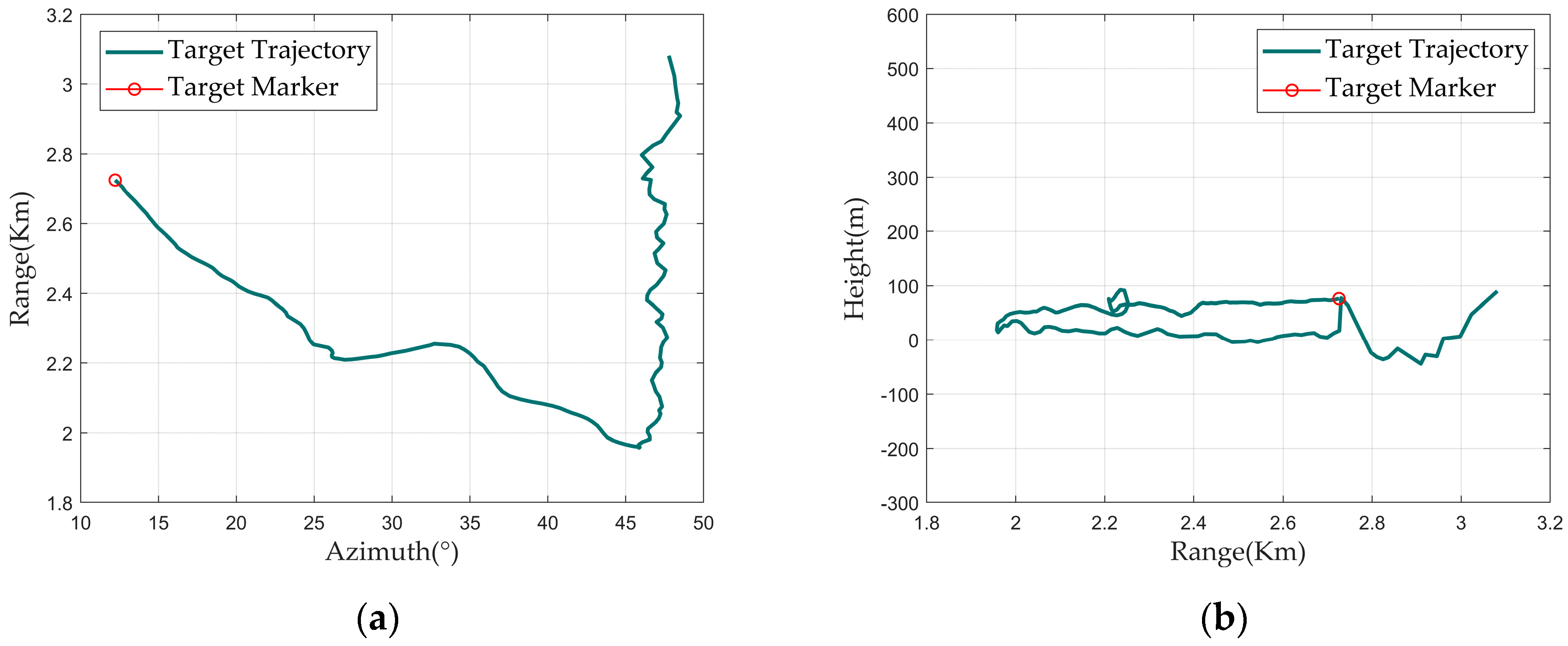
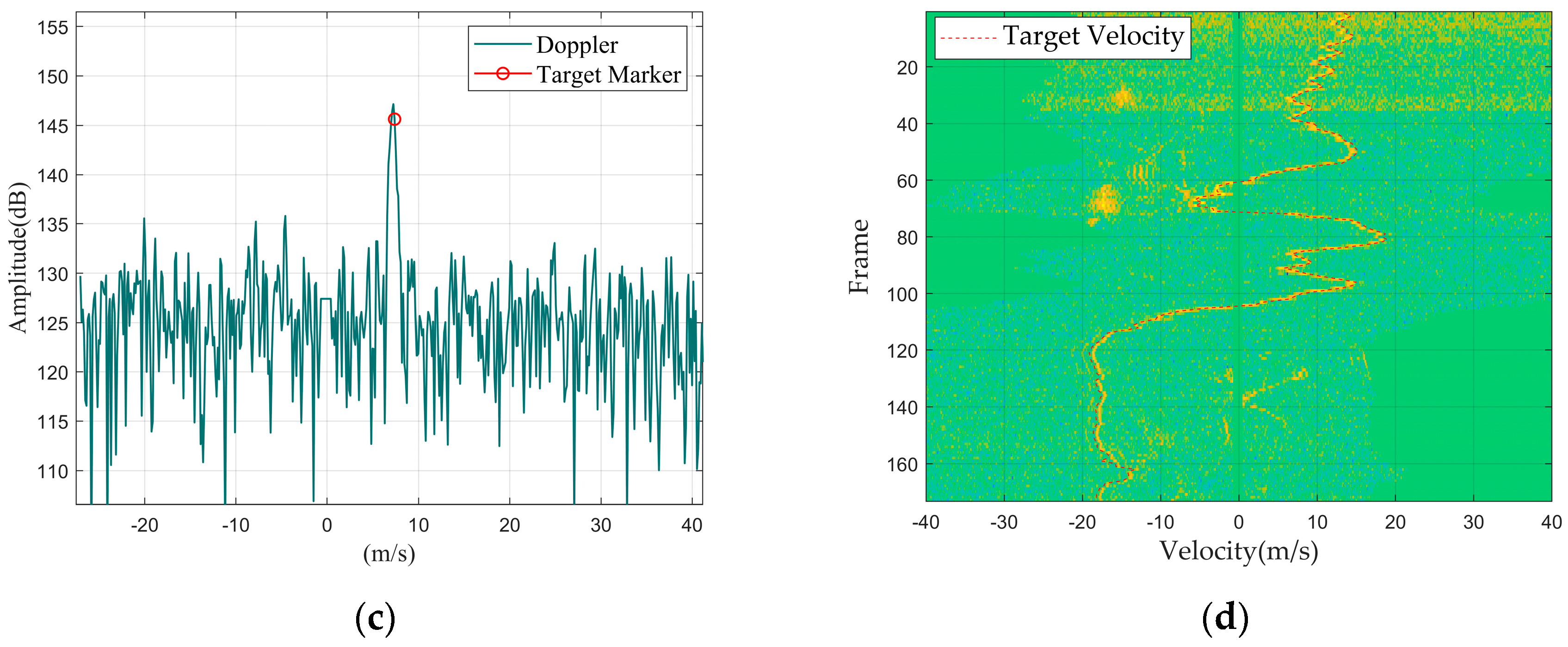
For TD data, the TD diagram can be used for intuitive visualization. The TD diagram includes the Doppler waveform graph, the Doppler waterfall graph, the range–azimuth graph, and the range–height graph, as shown in Figure 1.
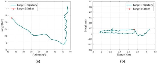

Figure 1.
TD diagram: (a) range-azimuth graph; (b) range-height graph; (c) Doppler waveform graph; and (d) Doppler waterfall graph.
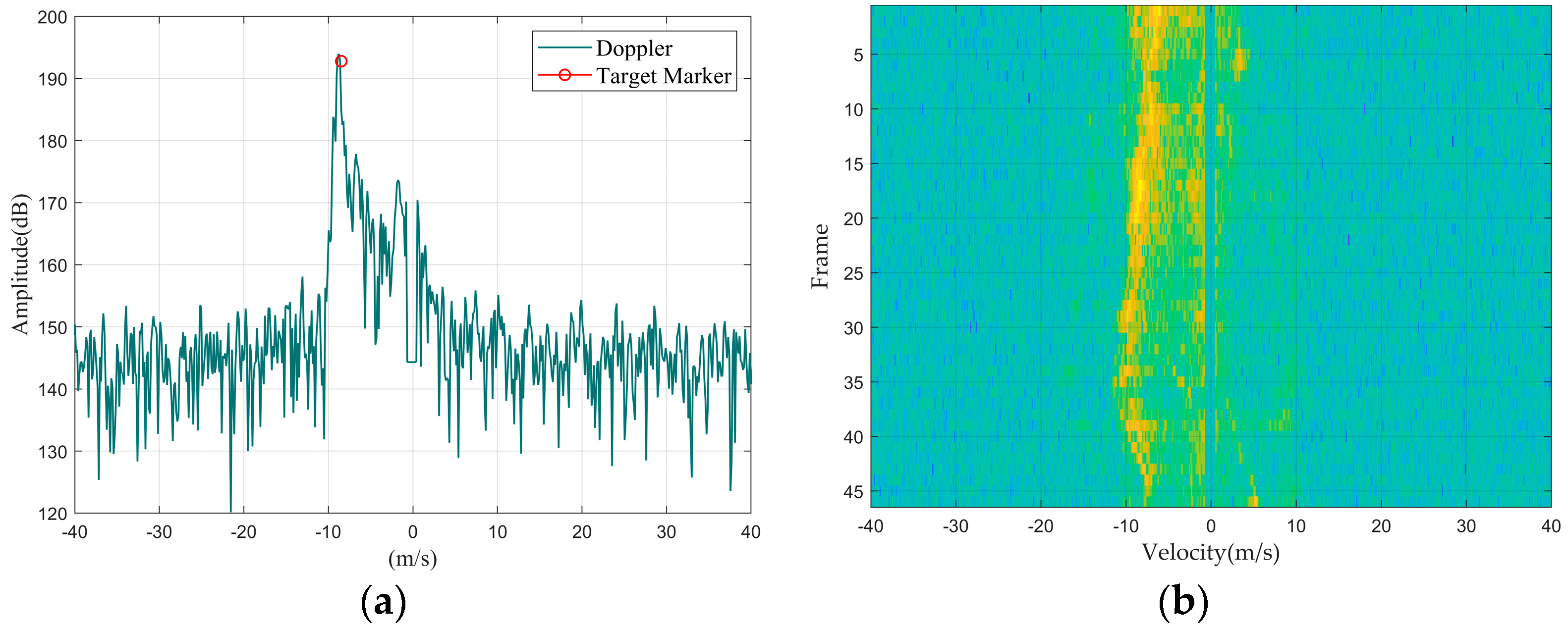
The X-axis of the Doppler waveform graph represents the radial velocity, and the Y-axis represents the amplitude. The value on the X-axis corresponding to the red circle indicates the current track point’s velocity.
The Doppler 1D data of all track points in a track form a Doppler 2D data. After conversion using an RGB color mapping matrix, a Doppler waterfall graph is formed. In this graph, the X-axis represents the target’s radial velocity, and the Y-axis represents the track point index, which can also be understood as the frame number or time. The brightness of the color in the Doppler waterfall graph indicates the amplitude of the corresponding Doppler 1D data. The red dashed line overlaid on the main Doppler spectrum connects the velocity values from the track information of each track point.
This section provides a detailed introduction to the composition of TD data using the TD diagram. The next section will provide a detailed introduction to the feature distribution of different targets within single-row Doppler data and between multiple rows of Doppler data.
2.2. Track Doppler of Different Targets
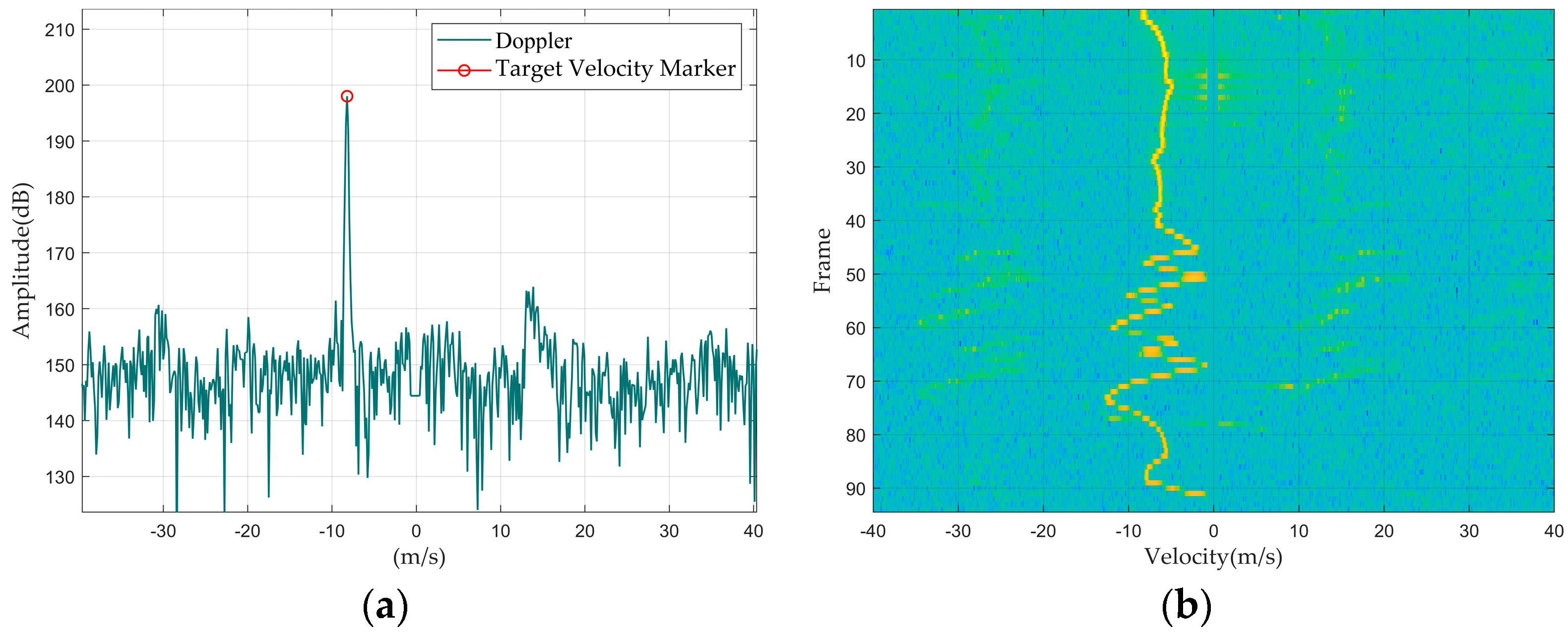
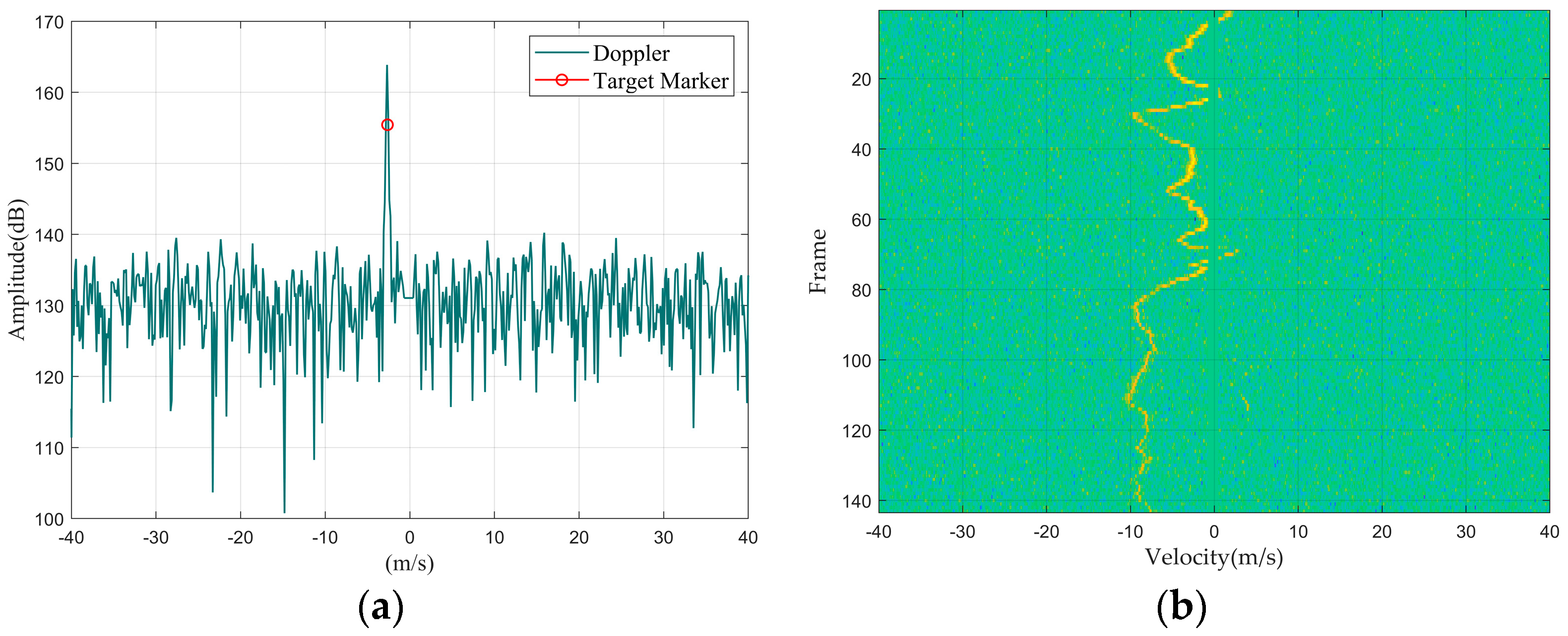
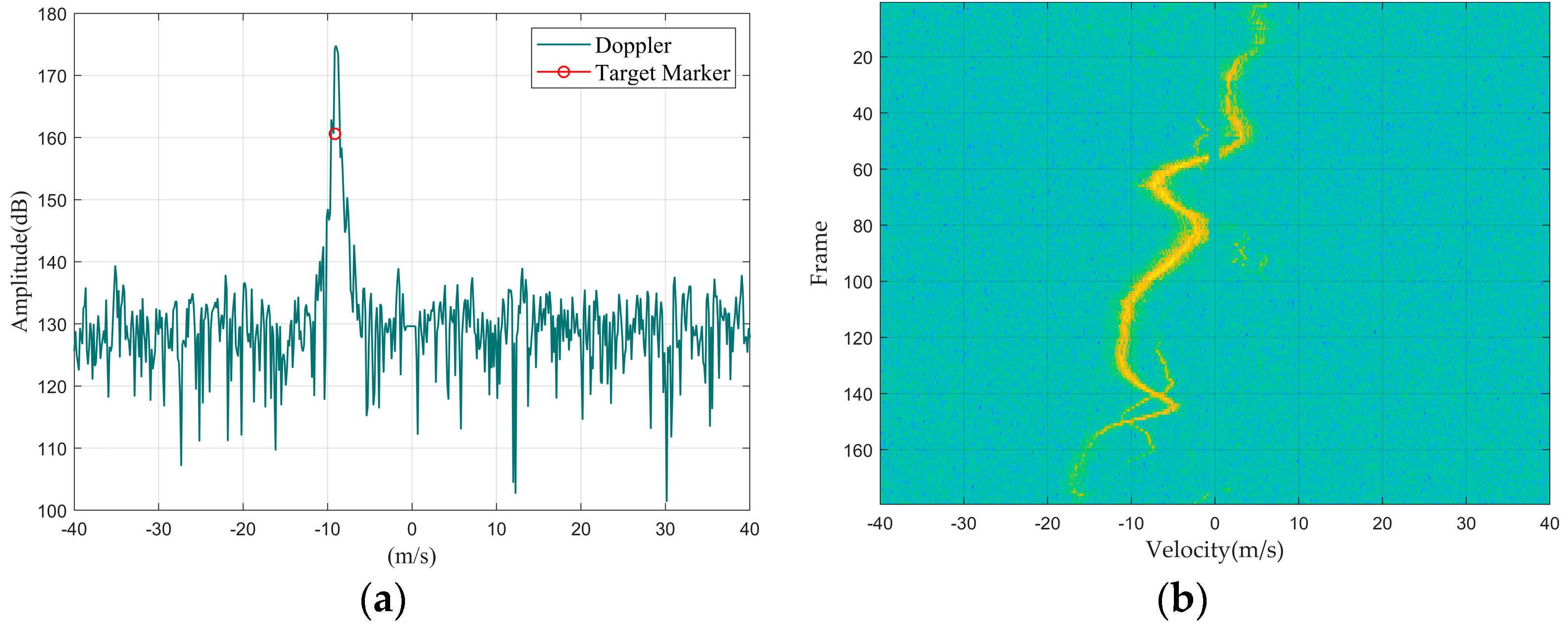
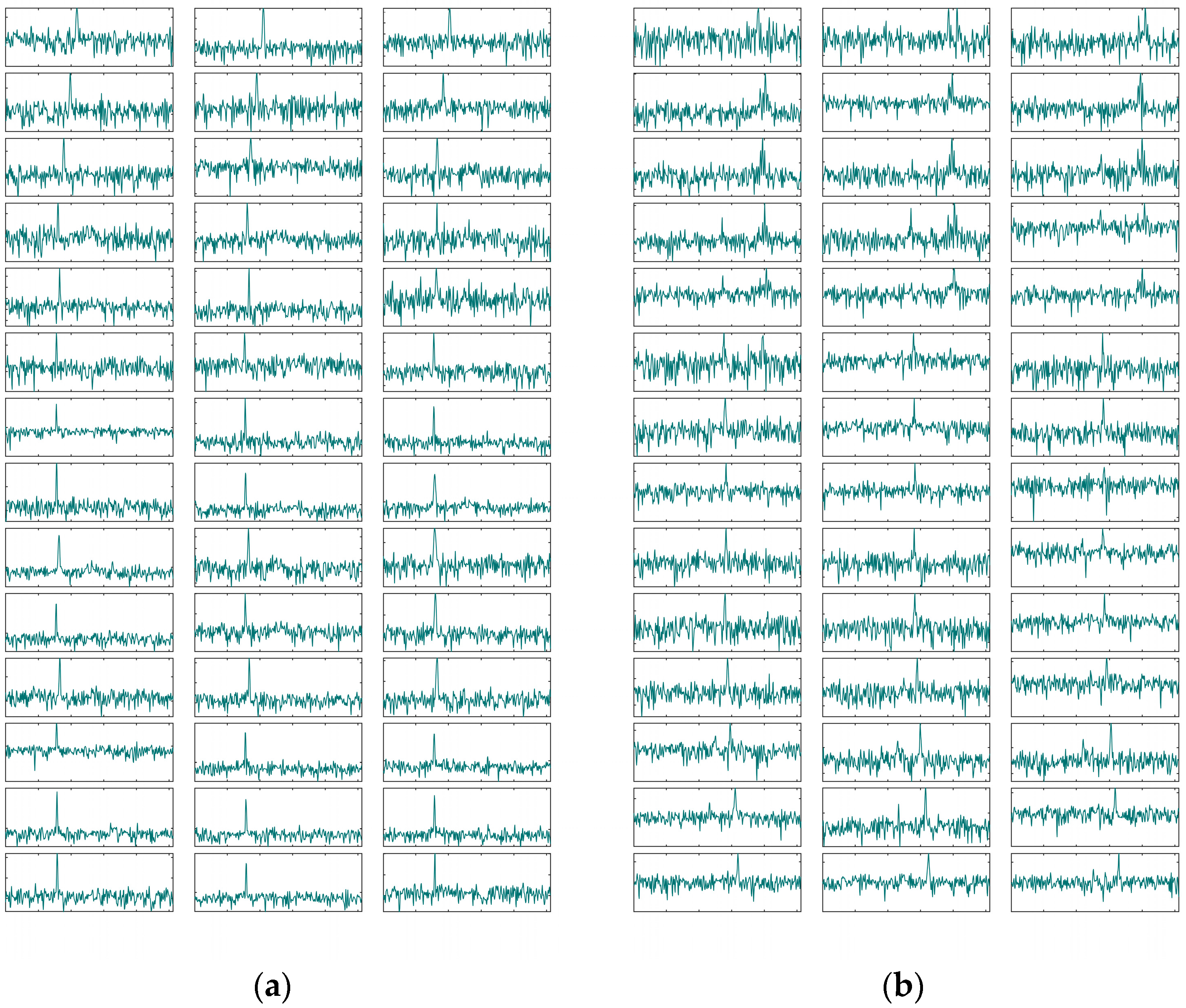
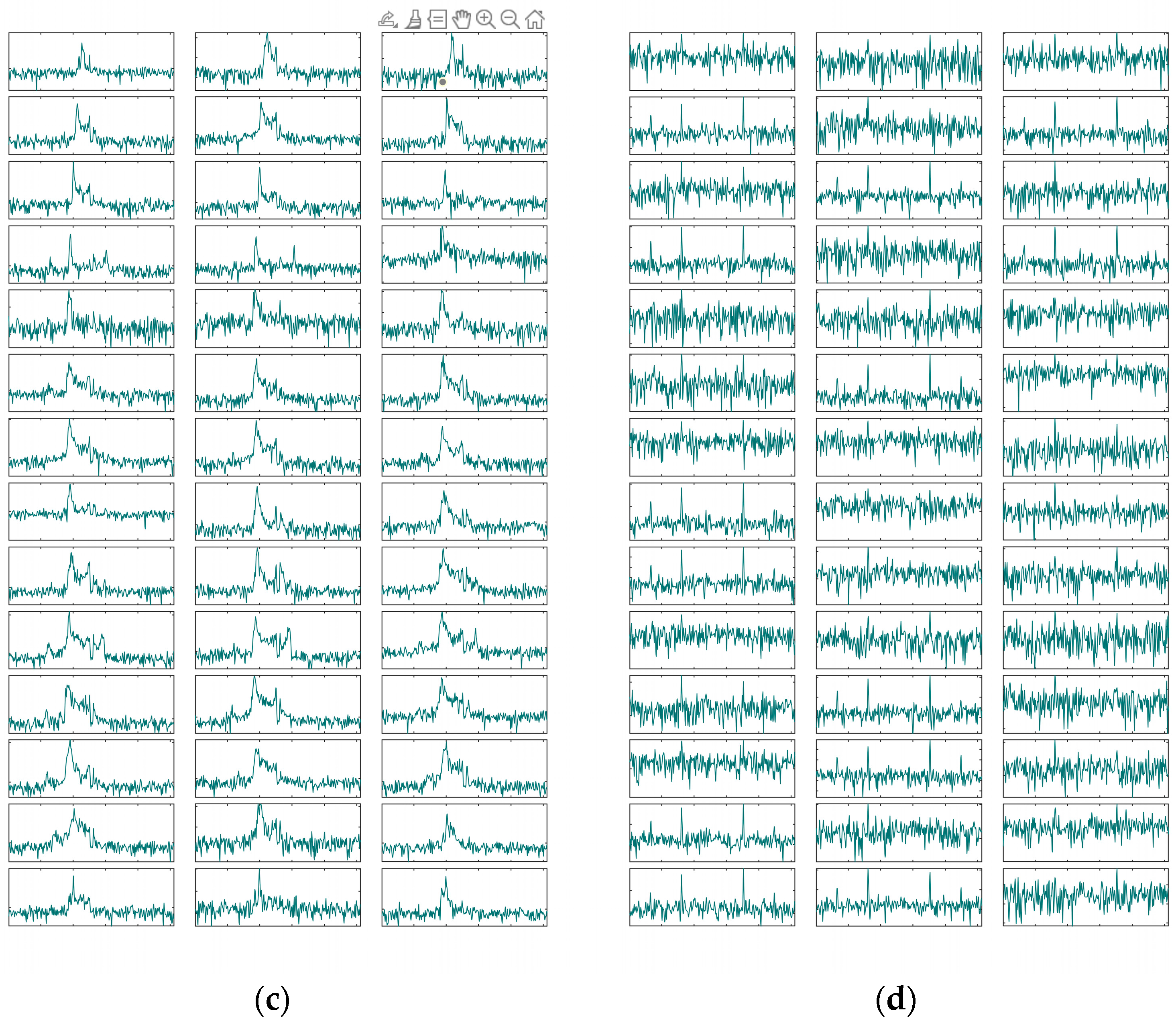
Since the classification in this paper uses sliding window Doppler data, this section will first present the Doppler waveform graphs and Doppler waterfall graphs of drones, birds, cars, and rotating targets. Based on this, this section will summarize the feature distribution within single-row Doppler 1D data for these four types of targets using the Doppler waveform graph and introduce the feature distribution between multiple rows of Doppler 1D data using the Doppler waterfall graph.
Summarizing Figure 2, Figure 3, Figure 4, Figure 5 and Figure 6, we identified the main features that comprise the four objectives categories.
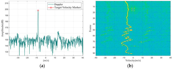
Figure 2.
Drone DJI Mavic 2: (a) Doppler waveform graph; (b) Doppler waterfall graph.

Figure 3.
Single bird: (a) Doppler waveform graph; (b) Doppler waterfall graph.
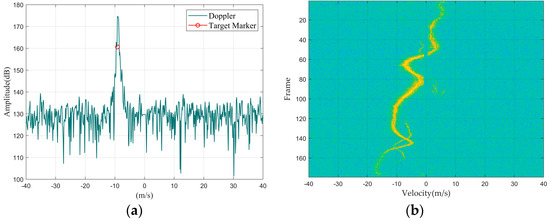
Figure 4.
Flock of birds: (a) Doppler waveform graph; (b) Doppler waterfall graph.
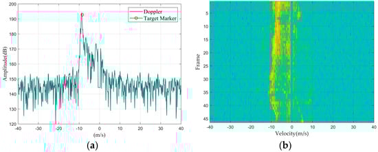
Figure 5.
Car: (a) Doppler waveform graph; (b) Doppler waterfall graph.
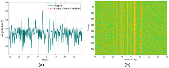
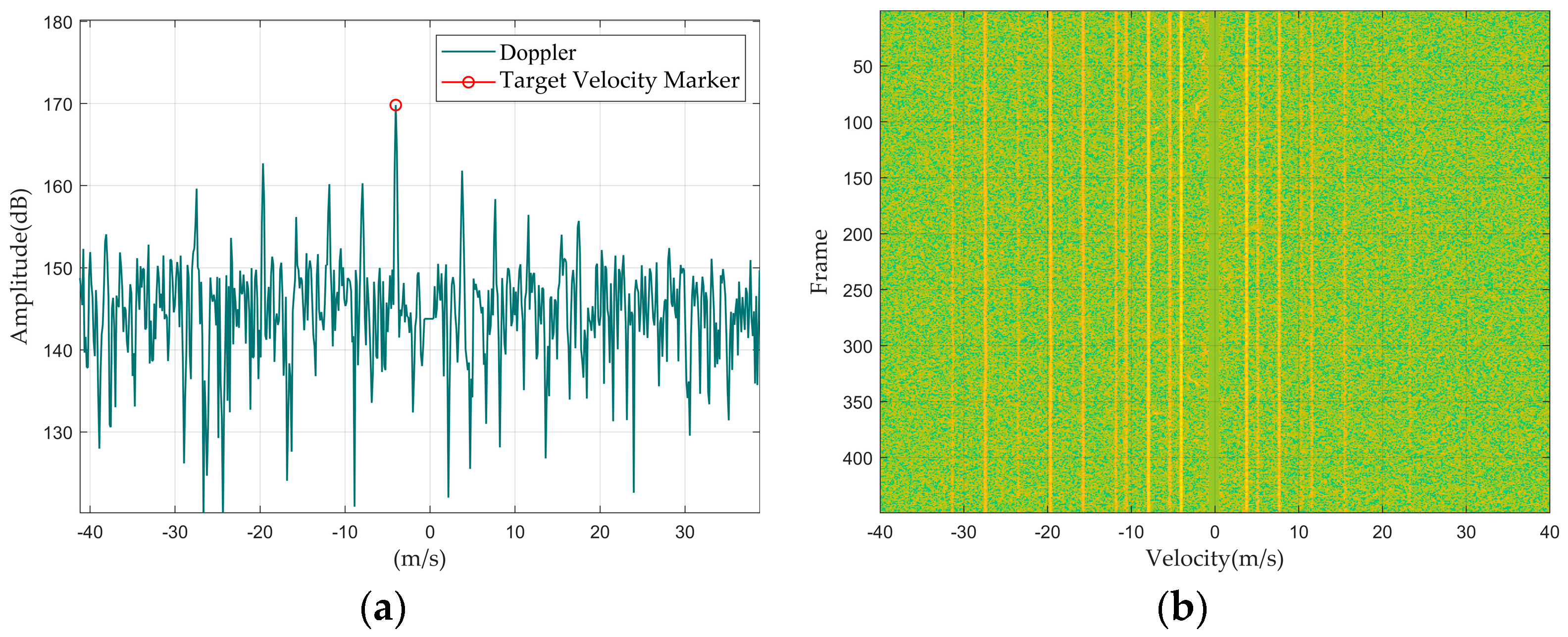
Figure 6.
Rotating target: (a) Doppler waveform graph; (b) Doppler waterfall graph.
First, we summarized the feature distribution of different targets from the perspective of Doppler 1D data, mainly discussing the amplitude, width, and shape of the main Doppler spectrum and the presence or absence of the micro-Doppler spectrum.
Regarding the main Doppler spectrum width, since the main Doppler spectrum width of multiple targets is greater than that of a single large target, the following situations can occur: the main Doppler spectrum width of a drone and a single bird are similar, but both are narrower than those of a bird flock and a vehicle; rotating targets do not have a main Doppler spectrum because the main body of the target is stationary.
In terms of the main Doppler spectrum amplitude, since a larger Radar Cross-Section (RCS) results in stronger reflected energy, the amplitude of the main Doppler spectrum will be larger. Therefore, the normalized signal-to-noise ratio of a vehicle and a drone is usually greater than that of a bird and a bird flock. Furthermore, in terms of the stability of the main Doppler spectrum amplitude over time, targets with relatively stable structures can generate stable reflection signals; so, the main Doppler spectrum amplitude of a vehicle and a drone tends to be more stable over time compared to that of a bird or bird flock.
As for the shape of the main Doppler spectrum, due to the large structural volume of a vehicle, different parts can generate different velocity states, resulting in spectral spreading around its main Doppler spectrum. Additionally, the closer the vehicle is to the radar, the more pronounced the spectral spreading becomes compared to other small targets.
As for micro-Doppler, since micro-Doppler is generated by rotating parts of the target and is symmetrically distributed relative to the main Doppler spectrum, the amplitude of the micro-Doppler spectrum is related to the target’s distance from the radar and the radar reflection capability of the rotating parts. For the dataset in this paper, medium to large drones within a distance of 1 km from the radar will exhibit a micro-Doppler spectrum, such as the DJI Inspire 2 and the DJI Mavic 2. Fixed objects like wind turbines or weather vanes will also produce a micro-Doppler spectrum; and since the fans of wind turbines or weather vanes are made of iron, the amplitude of their micro-Doppler spectrum will be significantly greater than that of drones.
Secondly, by summarizing the characteristic distributions of different targets from the Doppler waterfall graphs, since the position of the main Doppler spectrum represents the target’s velocity, the changes in the main Doppler spectrum position across multiple lines of Doppler 1D data represent the target’s maneuverability. Among the four types of targets, the speed variations in drones and vehicles are relatively stable, whereas bird targets, due to their agile movement patterns, exhibit relatively larger fluctuations in speed variation. Therefore, it can be concluded that the maneuverability of drones and vehicles is lower than that of birds.
This section first presents the one-dimensional Doppler spectrum and Doppler waterfall diagram for four types of targets, summarizing their characteristic distributions in these two aspects. Firstly, different targets show distinctions in terms of the main Doppler spectrum width, main Doppler spectrum amplitude, presence or absence of main Doppler spectrum extension, and presence or absence of micro-Doppler signatures within the one-dimensional Doppler data. Secondly, since the changes in the position of the main Doppler spectrum across multiple lines represent the target’s maneuverability, different targets will also exhibit differences in maneuverability.
The subsequent two sections will design a real-time processing workflow for ubiquitous radar data based on the characteristic distributions within and across lines and will design a classifier that can simultaneously capture both intra-line and inter-line features.
3. Data Preprocessing
3.1. Radar Operating Modes
The radar operating modes of a ubiquitous radar are shown as follows:
From Figure 7, it can be seen that the ubiquitous radar belongs to a track-then-identify (TTI) radar system. This means that, after associating plot tracks and forming the trajectory, it then performs target identification. By adopting this TTI operating mode, the system can extend the trajectory points frame by frame. Using the distance information of the trajectory points, it obtains a one-dimensional high-resolution Doppler spectrum of the range cell on the range–Doppler (RD) plane, thereby greatly enhancing target identifiability [25]. Based on the radar operating mode described in this section, the next section will detail the data processing flow of the ubiquitous radar.
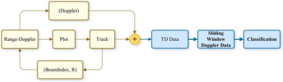
Figure 7.
Ubiquitous radar tracking and identification process.
3.2. Real-Time Classification Process
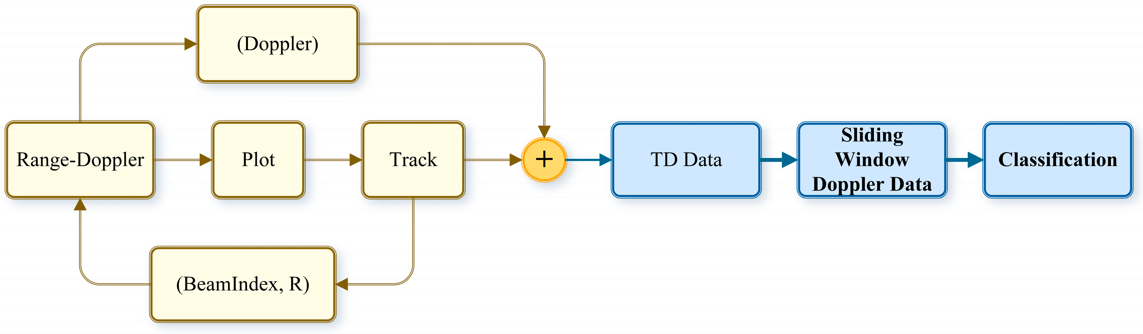
The real-time classification process for the ubiquitous radar based on sliding window Doppler data is shown in Figure 8.
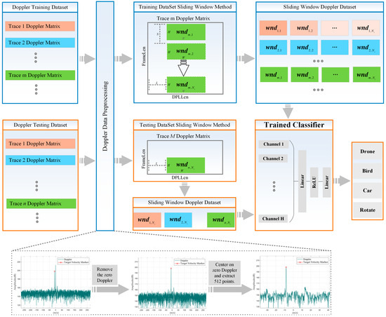
Figure 8.
Real−time classification process of ubiquitous radar.
From Figure 8, it can be seen that the data processing flow of the ubiquitous radar mainly consists of three parts: training set data processing flow, test set data processing flow, and Doppler data preprocessing. In what follows, we explain each part in detail:
First is the Doppler data preprocessing, which includes two parts: zero Doppler smoothing and Doppler clipping. Both the training set data and the test set data need to experience this process. In zero Doppler smoothing, the mean amplitude value of the high-frequency region is taken and then used to replace the amplitude values near the zero Doppler. For Doppler clipping, since this paper focuses on LSS targets whose speeds generally fall within a specific speed range , the Doppler 1D data are clipped according to this speed range.
Secondly, the data processing flow for the training set is as follows: After preprocessing the Doppler 2D data of all tracks in the dataset, the length of the x-axis of each track’s Doppler 2D data is , and the length of the y-axis is . The sliding window size on the x-axis and the size on the y-axis are defined. The window is symmetric about zero Doppler and traverses the entire track with a step size . Using the same method to traverse all tracks in the training dataset, a training dataset is ultimately formed, and a classification network is trained using the testing dataset.
The processing flow for the test dataset is similar to that of the training set, with the only difference being the parameters of the sliding window. To more accurately simulate the actual operation of the radar, the sliding window needs to gradually move forward as the track extends; so, the step size of the sliding window is set to 1. The test dataset includes the Doppler data of the sliding window corresponding to the latest track points of all tracks. Once the test dataset is formed, it is fed into the trained classifier, which ultimately outputs the target categories of all the latest track points.
In this section, we detail the data processing flow for real-time classification based on the working mode of the ubiquitous radar. The core of this process is to ensure that the network receives sufficient feature input while minimizing the number of Doppler rows fed into the network, all while meeting real-time classification requirements. Since the ubiquitous radar primarily focuses on low-speed targets, Doppler 1D data are truncated and processed. Based on these principles, Doppler sliding window technology is used to generate data. This real-time classification process not only reduces the amount of data required for classification but also significantly improves the efficiency of real-time classification, ensuring the high performance of the system with a low latency.
4. Classifier Design
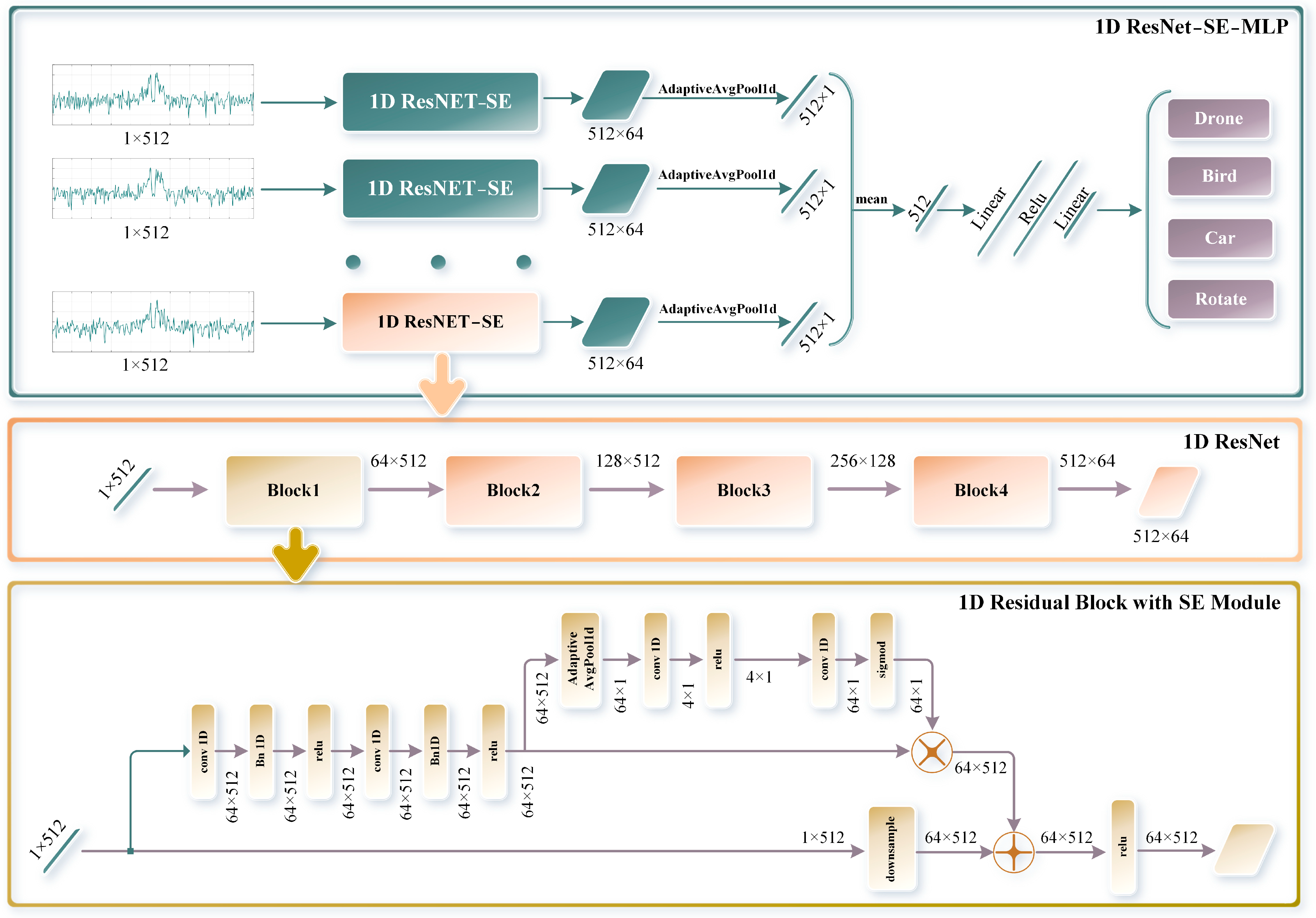
The multi-channel parallel network, as shown in Figure 9, uses sliding window Doppler data for target classification. The network structure is illustrated in the figure, progressing from overall to specific details: the overall diagram of the 1D ResNet-SE-MLP multi-channel network, the diagram of the single-channel 1D ResNet network [26], and the diagram of the residual block with the 1D SE attention module [27].
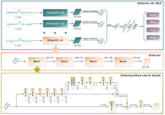
Figure 9.
Multi-channel parallel network architecture diagram.
- Overall Diagram of the 1D ResNet-SE-MLP Multi-channel Network:
The multi-channel network is composed of multiple feature extraction channels based on 1D ResNet-SE, each processing one row of high-resolution Doppler data within a sliding window, with each row having a length of 512. The feature extraction results from each channel are dimensionally reduced through adaptive average pooling. All channel features are then merged into a one-dimensional vector by averaging, which is subsequently passed to the classifier. The classifier, composed of multiple linear layers and ReLU activation functions, forms a multi-layer perceptron (MLP) capable of outputting four classification results: drone, bird, car, and rotating target.
- Overall Diagram of the Single-channel 1D ResNet-SE Network:
Each channel contains an independent 1D ResNet-SE network that extracts features from the input one-dimensional high-resolution Doppler data of length 512. The 1D ResNet-SE network extracts features through multiple residual blocks. These residual blocks utilize 1D convolutional layers to perform convolution operations on the input data and adjust the inter-channel weights through the SE module, enhancing the feature representation capability and network robustness.
- Overall Diagram of the Residual Block with 1D SE Attention Module:
Each residual block consists of multiple 1D convolutional layers, a 1D SE module, and skip connections, enabling the network to more effectively learn features. The 1D SE module operates in two main steps: ‘Squeeze’ and ‘Excitation’.
Squeeze: Global average pooling is used to compress the spatial information of each feature channel into a scalar, obtaining a global description for each channel.
Excitation: A 1D convolutional layer reduces the number of channels, followed by ReLU activation. Another 1D convolutional layer then restores the original number of channels. The sigmoid activation function is used to normalize the weight coefficients for each channel. Finally, these weight coefficients are applied to the original feature map to enhance important features and suppress less important ones, thereby improving the classification performance.
Specifically, the residual block performs convolution operations on the input data through 1D convolutional layers and retains the original information of the input features via skip connections. With the additional weighted processing of the 1D SE module, the residual block can more effectively capture and represent key features.
5. Results and Discussion
5.1. Experimental Environment
5.1.1. Ubiquitous Radar Parameters
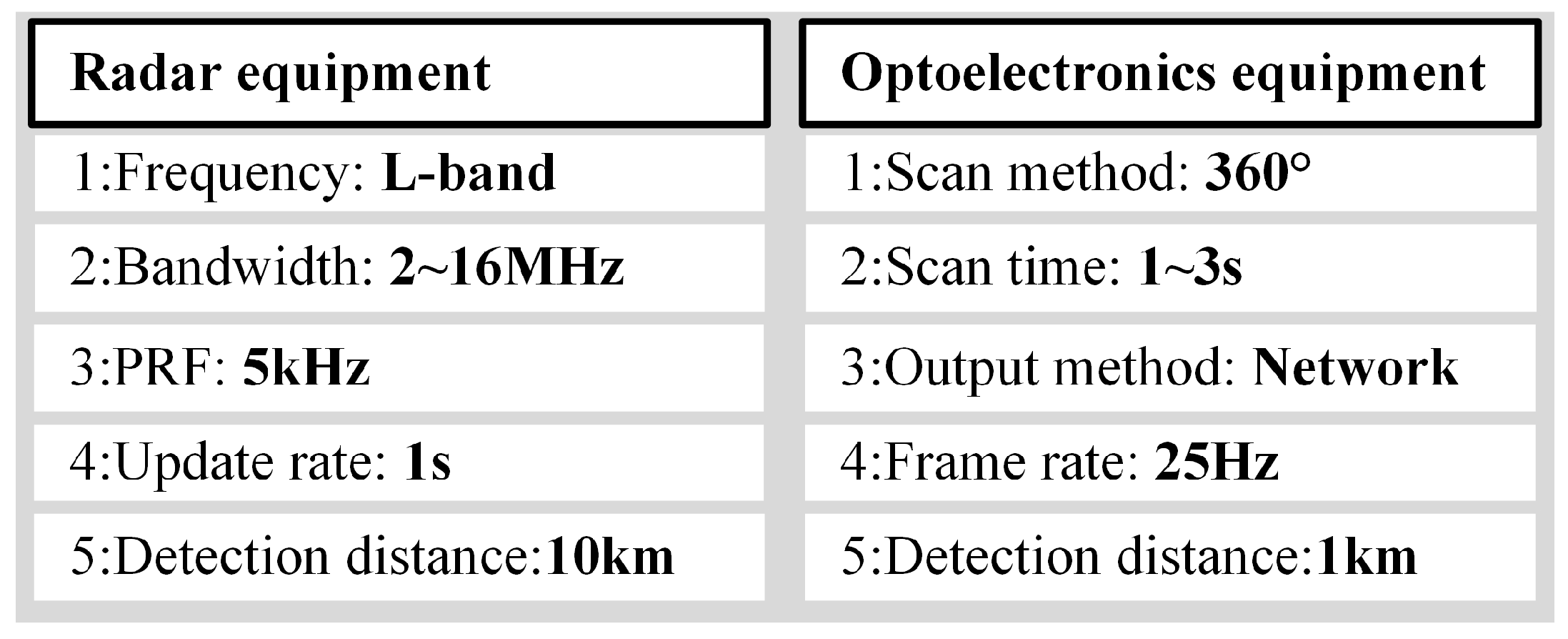
The main parameters of the ubiquitous radar are shown in Figure 10.

Figure 10.
Radar parameters.
The radar equipment employs a wide-beam transmitting antenna, which can cover a 90° azimuth sector centered on the antenna’s line of sight. The receiving antenna consists of multiple grid-structured sensors [28,29]. Digital beamforming technology is utilized to create multiple receiving beams while capturing echo data, covering the entire monitored scene. The electro-optical equipment can receive guidance from the radar equipment and detect and track targets. When used in conjunction, these systems can efficiently detect, warn, and provide evidence for LSS targets [30,31].
5.1.2. Computer Specifications
The computer used for training the network was sourced from Lenovo, located in Guangzhou, China. It was equipped with an Intel i7-13700KF CPU, 32 GB of memory running at 4400 MHz, and 1 TB of storage. It featured an NVIDIA GeForce RTX 4090D GPU. The development environment included PyCharm version 2023.3.6 as the integrated development environment (IDE), PyTorch version 2.2.1 for the deep learning library, and CUDA version 11.8.
5.2. Dataset Composition
The dataset used in this paper mainly comprises four types of objects: drones, birds, cars, and rotating targets. The specific composition of the dataset is shown in Table 1. It is important to note that different sliding window parameters can lead to variations in dataset quantities. The table below illustrates the composition of the dataset with the optimal window parameters selected for this study (window size of 10 and sliding step size of 6).

Table 1.
Dataset composition.
To ensure dataset diversity, the target categories included four drone models (DJI AVATA, DJI Air, DJI Mavic, and DJI Inspire), three bird types (single birds, flocks of birds, and flapping birds), common vehicle targets from the test site’s roads, and several fixed-position rotating targets. The data collection sites for drones, cars, and rotating targets were the same, while bird targets were collected from different locations. Additionally, the data collection occurred at different periods for each target type.
To better understand the dataset composition, thumbnails are displayed in Figure 11.
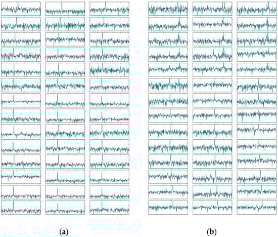
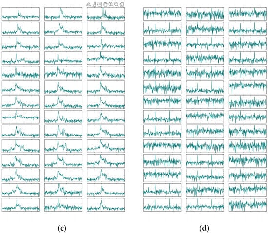
Figure 11.
Dataset thumbnails: (a) drones; (b) birds; (c) cars; (d) rotating targets.
5.3. Backbone Network Selection for Feature Extraction Module
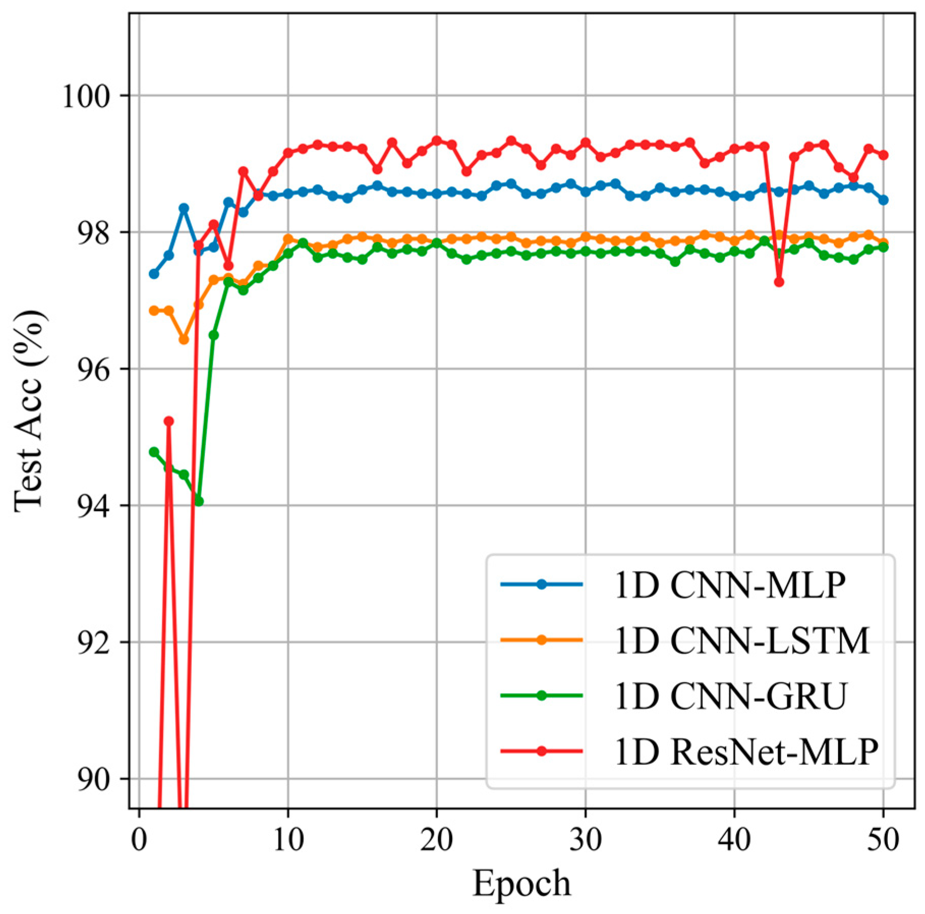
Based on the dataset introduction in the previous section, this section compares the classification results of four commonly used multi-channel classification networks to select a suitable feature extraction module for sliding window Doppler data. The four networks are 1D CNN-MLP [15], 1D CNN-LSTM [23], 1D CNN-GRU [16], and 1D ResNet-MLP. The classification results of the four networks are shown in Figure 12 and Table 2.
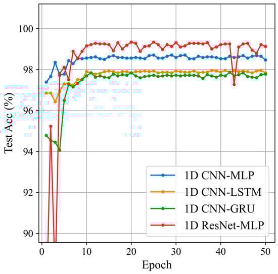
Figure 12.
Classification results of the different feature extraction modules.
Table 2.
Classification results of the different feature extraction modules.
The 1D ResNet-MLP network achieved the highest classification accuracy, reaching 99.34%, and also excelled in precision, recall, and F1 score, demonstrating its superior performance and stability in feature extraction and classification tasks. Although the other models (1D CNN-MLP, 1D CNN-LSTM, and 1D CNN-GRU) performed well, they did not match the performance of the 1D ResNet-MLP. The comparison between 1D CNN-MLP and 1D ResNet-MLP networks clearly shows the significant advantage of using 1D ResNet as the backbone network for the feature extraction module.
5.4. Feature Fusion Module Selection
Building on the previous section, this section will compare two different feature fusion modules to select the one most suitable for sliding window Doppler data. The feature fusion modules are MLP, GRU, and LSTM [32]. The classification results are shown in Figure 13 and Table 3.
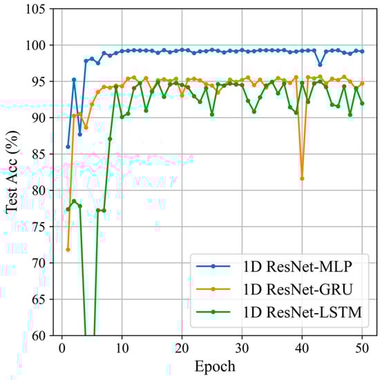
Figure 13.
Classification results of the different feature fusion modules.
Table 3.
Classification results of the different feature fusion modules.
The experimental results indicate that, using 1D ResNet as the base network, the model with MLP as the feature fusion module performs the best, achieving an accuracy of 99.34%. It also excels in precision, recall, and F1 score, demonstrating superior performance and stability in feature extraction and classification tasks. In comparison, models using GRU and LSTM as feature fusion modules also perform well but fall short of MLP in all metrics. This indicates that using MLP as the feature fusion module on the 1D ResNet base network has significant advantages.
5.5. Window Parameter Selection
Based on the network structure determined in the previous section, this section will select the optimal parameter combination by changing the sliding window parameters, specifically the window size and the sliding window step size.
- Sliding Window Length Selection
Firstly, we set the window size to 10 and started with a sliding window step size of 2, incrementing by 2 up to 10. We compared the classification results with different sliding window step sizes. The classification results are shown in Figure 14 and Table 4.

Figure 14.
Classification results by sliding window step sizes.
Table 4.
Classification results by sliding window step sizes.
From the classification results, it can be seen that, compared to sliding window step lengths of 6, 8, and 10, the step lengths of 2 and 4 have higher accuracy. However, the standard deviation indicates that the stability and consistency of step lengths 2 and 4 are relatively poor. Among the step lengths of 6, 8, and 10, a step length of 6 offers higher stability and consistency, and also achieves the highest accuracy among the three. Considering both stability and accuracy, this paper selected a window size of 10 and a sliding window step length of 6.
- Sliding Window Size Selection
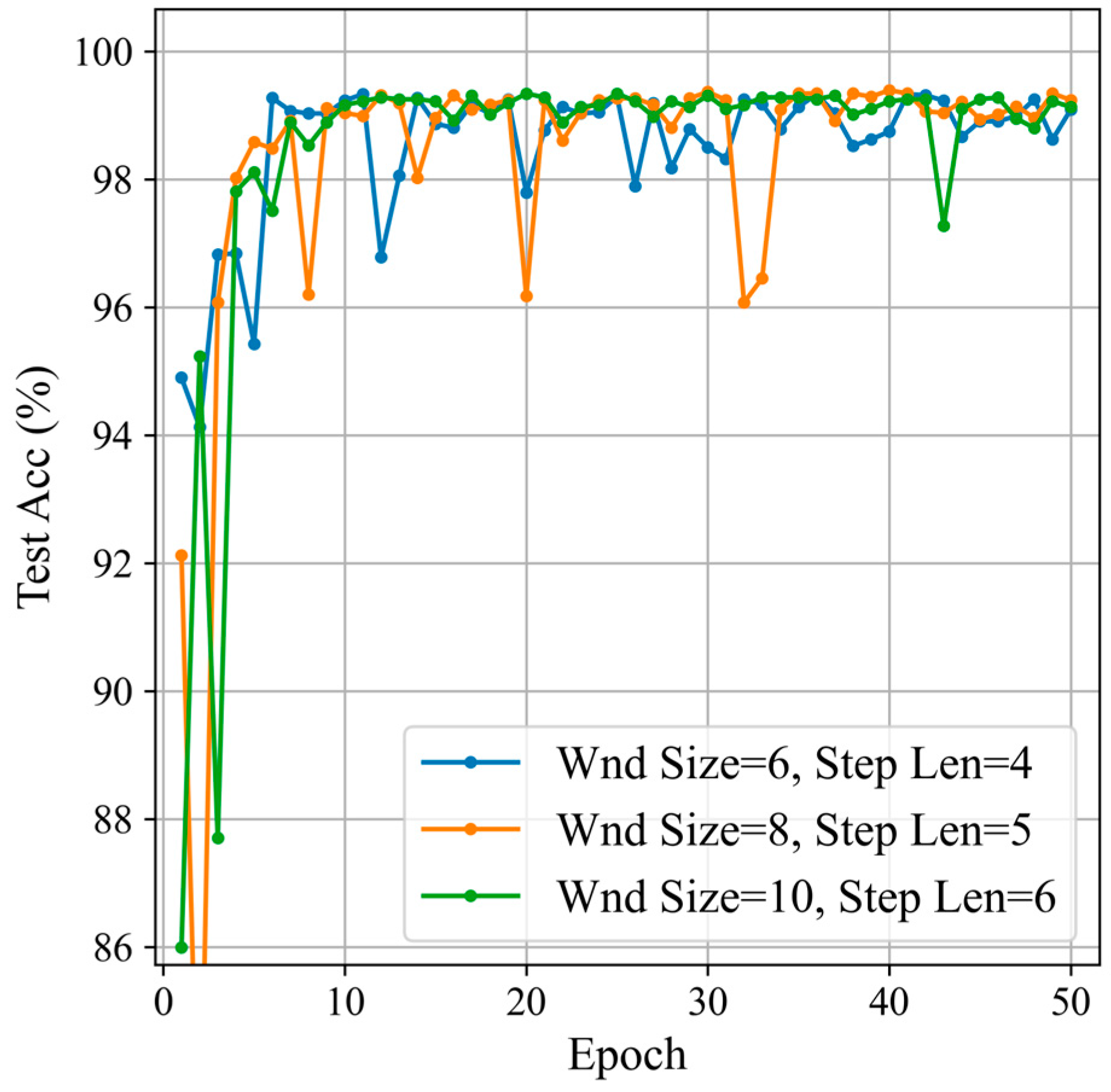
Based on the optimal sliding window step length and size ratio determined in the previous section, this section sets three groups of parameters with window sizes of 10, 8, and 6, respectively. The classification results are compared to select the best smaller window size, as shown in Figure 15 and Table 5.
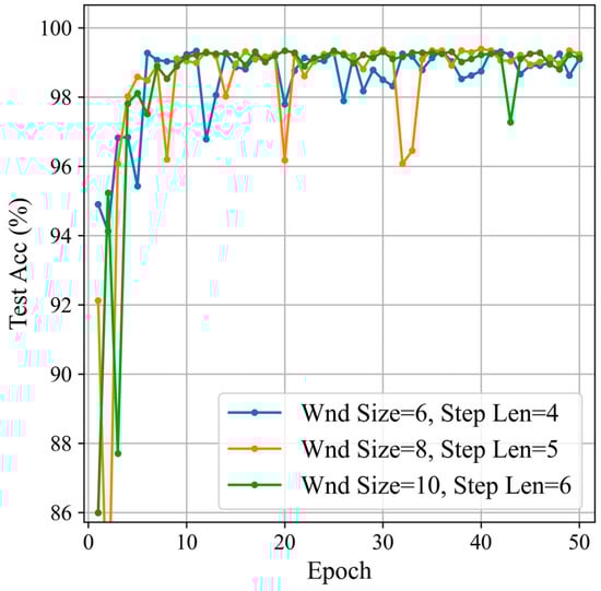
Figure 15.
Classification results for different window sizes.
Table 5.
Classification results for different window sizes.
By comparing the classification performance of different sliding window sizes and step length combinations, it can be seen that, when the window size is 8 and the step length is 5, the precision, recall, and F1 score are the highest, but the standard deviation is also the largest, indicating a greater variability in model performance across different training epochs. When the window size is 10 and the step length is 6, although the precision, recall, and F1 score are not as high as with the window size of 8 and step length of 5, the standard deviation is the smallest, indicating the best model stability. Considering both accuracy and stability, the combination of a window size of 10 and a step length of 6 performs the best.
5.6. Attention Module Selection
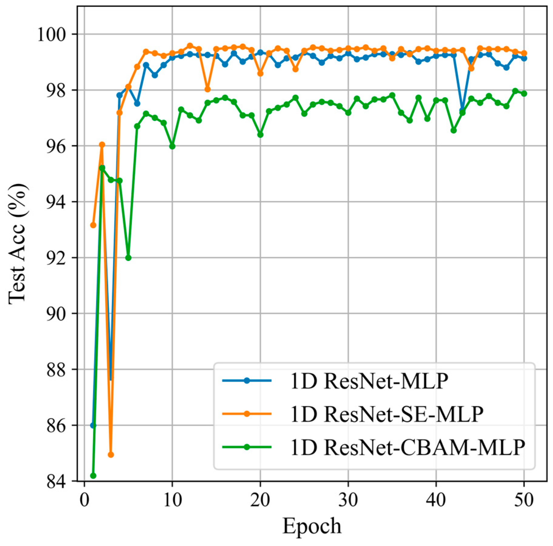
Based on the optimal sliding window parameters from the previous section, this section will compare the impact of different attention modules on the classification results. The attention modules being compared are 1D CBAM [33] and 1D SE, as shown in Figure 16 and Table 6.

Figure 16.
Classification results for the different attention modules.
Table 6.
Classification results for the different attention modules.
Based on these results, we can conclude that introducing the 1D SE module into the 1D ResNet network significantly improves classification performance. This indicates that the 1D SE module has considerable advantages in feature extraction. The SE module enhances the model’s attention to important features through the “Squeeze” and “Excitation” operations, adaptively reweighting each feature channel.
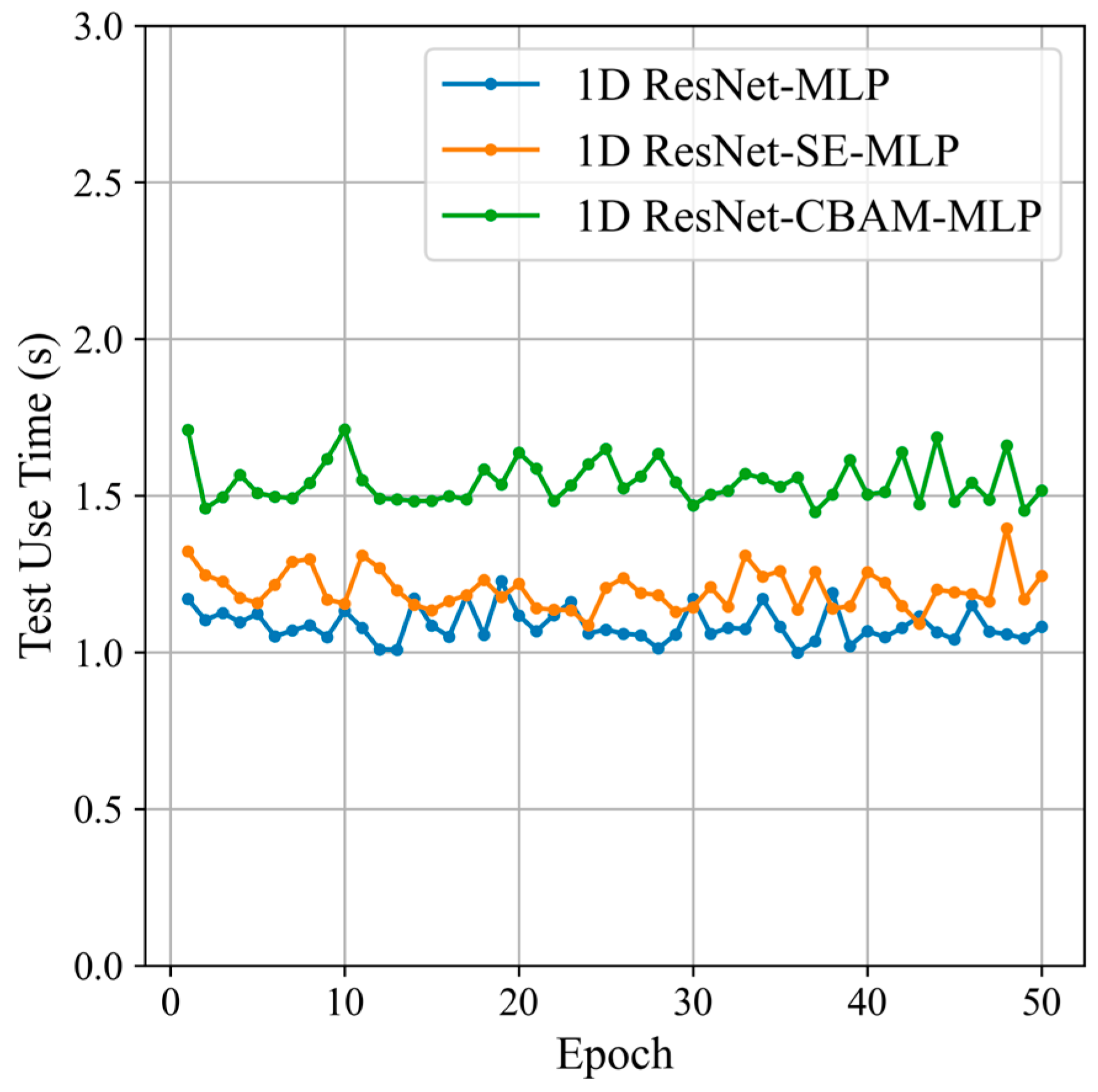
Based on the computer specifications in Section 5.1.2 and the size of the test set in Table 1, we recorded the classification times of three types of networks on the test set, as shown in Figure 17.
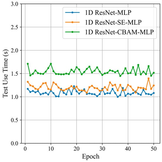
Figure 17.
Classification time of the different attention modules.
Figure 17 shows that the average classification time of the 1D ResNet-SE-MLP network on the test set is approximately 1.3 s. Compared to the 1D ResNet-CBAM-MLP network, the 1D ResNet-SE-MLP network achieves higher accuracy with shorter classification time. Furthermore, since the number of samples in the test set far exceeds the number of samples processed per frame update, all three networks meet the real-time classification requirements regarding classification time under the computer specifications used in this experiment. Considering both classification accuracy and time, the 1D ResNet-SE-MLP network demonstrates the best overall performance. The target recognition module generated by this network can provide an extended processing time for other radar signal processing functions, such as data preprocessing, target detection, and track association, within a single data update cycle.
Next, we will further demonstrate the impact of adding the 1D SE module on target classification through confusion matrices and class curves, as shown in Figure 18.
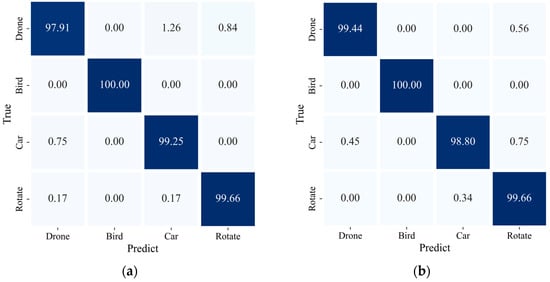
Figure 18.
Confusion matrices for the different attention modules: (a) 1D ResNet-MLP; (b) 1D ResNet-SE-MLP.
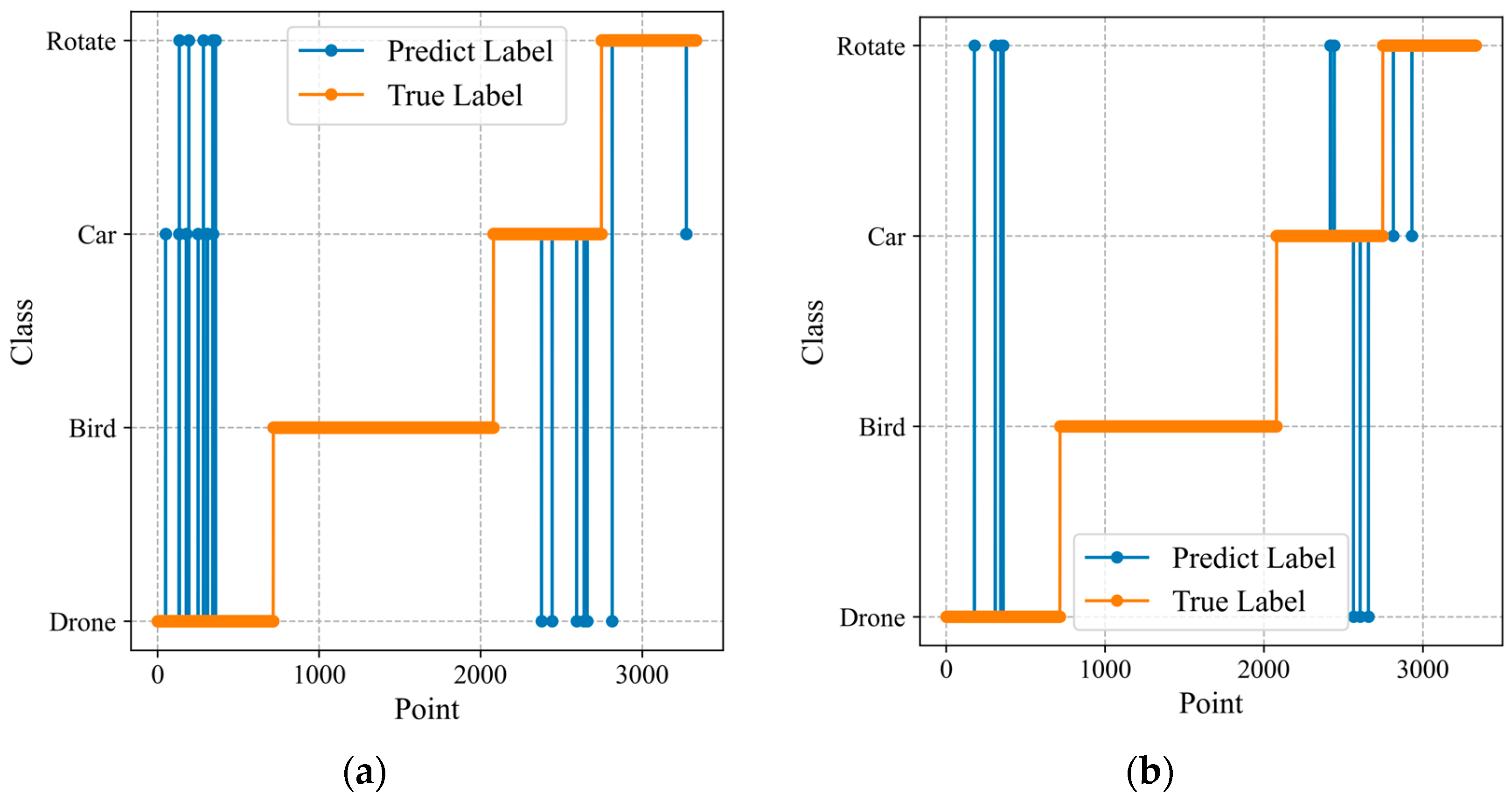
From the confusion matrix, it can be seen that the addition of the 1D SE module significantly improves the classification accuracy for drone targets, which are of particular concern in the LAE, from 97.91% to 99.44%. This improvement in the classification performance is also evident in the class curves, as shown in Figure 19.
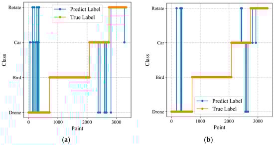
Figure 19.
The accuracy curves for different attention modules: (a) 1D ResNet-MLP; (b) 1D ResNet-SE-MLP.
Comparing the class curves of the two types of networks, it is evident that, after adding the 1D SE attention module, especially for the drone category, the number of false alarms and the number of missed detections significantly decreased.
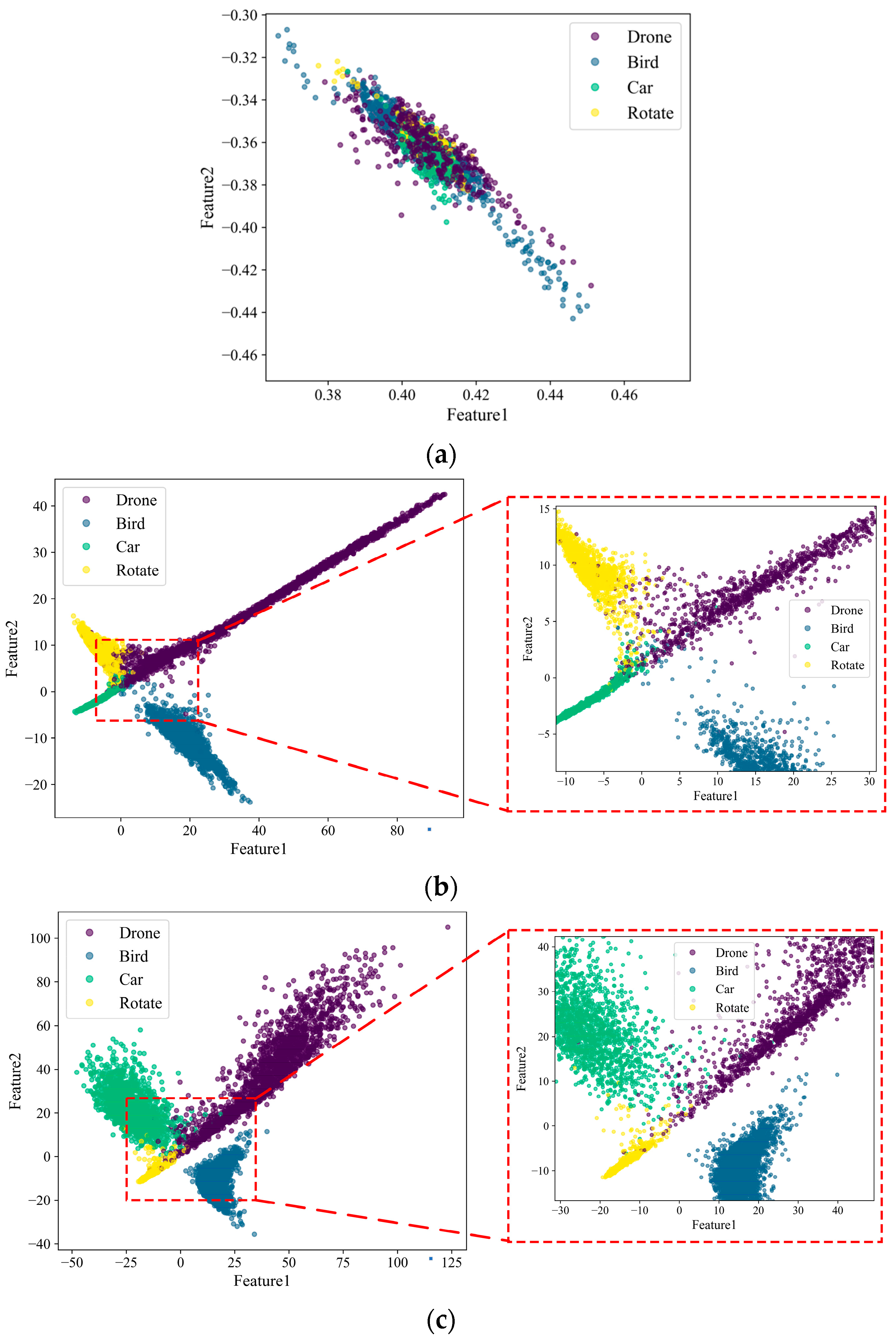
Finally, feature distribution diagrams are used to demonstrate the impact of adding the 1D SE module on target classification results. After the initial fully connected layer outputs of both networks, a fully connected layer with an output dimension of 2 is added to further compress the initial features into a two-dimensional space for ease of visualization and analysis. As shown in Figure 20, the feature distributions of the two networks, 1D ResNet-MLP and 1D ResNet-SE-MLP, are compared.
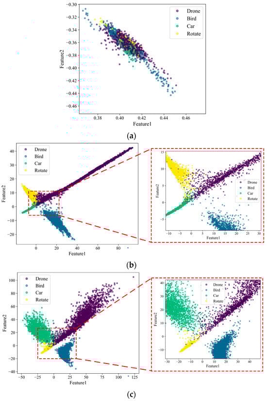
Figure 20.
The feature distribution for different attention modules: (a) Before training; (b) 1D ResNet-MLP; (c) 1D ResNet-SE-MLP.
Figure 20 shows that the feature distribution of the 1D ResNet-MLP is relatively dispersed, with a certain degree of overlap between different categories in the two-dimensional space, especially among drones, cars, and rotating targets. In contrast, the feature distribution of the 1D ResNet-SE-MLP is more concentrated, with different categories of feature points being more clearly separated and with less overlap. The network with the attention mechanism shows significant advantages in feature extraction and classification tasks. The attention mechanism not only improves the separability and concentration of features but also reduces the overlap between different categories, thereby enhancing the accuracy and robustness of classification.
In summary, this section discusses the classification performance of the 1D ResNet-MLP and 1D ResNet-SE-MLP networks from four perspectives: overall accuracy, confusion matrix, class curves, and feature distribution. Based on these analyses, it is concluded that the 1D SE attention module can enhance the model’s focus on important features, thereby improving classification accuracy.
5.7. Classification Results’ Presentation
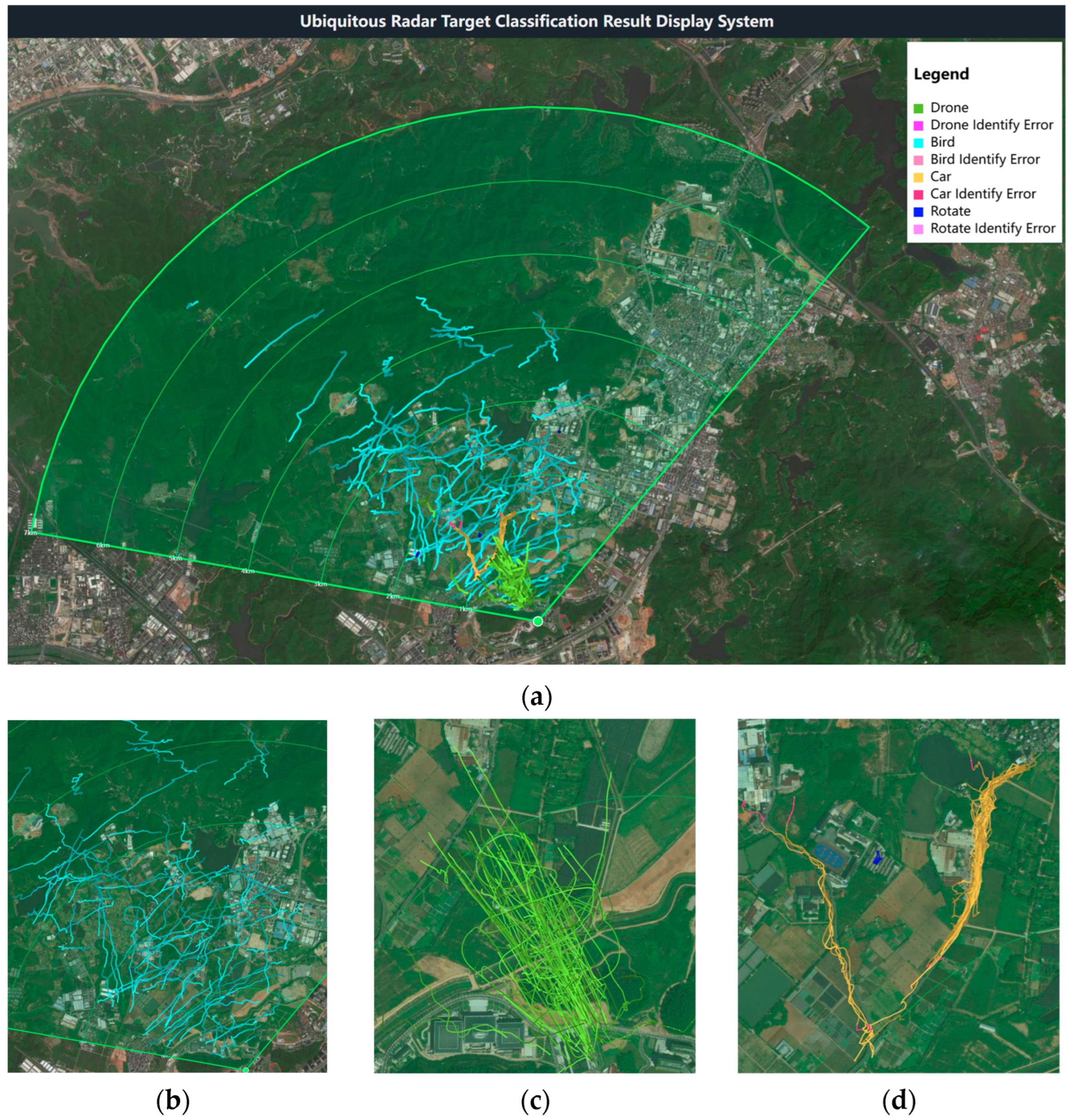
Finally, using the Amap API and Python, the target trajectories of the test set were parsed into map path data and embedded into an HTML static page for visualization, as shown in Figure 21.
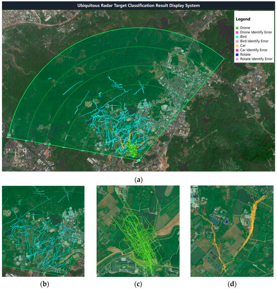
Figure 21.
Classification results: (a) overall; (b) birds; (c) drones; (d) cars and rotating targets.
The green color represents drones, light blue represents birds, yellow represents cars, and dark blue represents rotating targets. Misclassified targets in each category are indicated by different shades of red. Each trajectory uses a gradient of the same color from dark to light, with the direction of the gradient representing the direction of the target’s movement. Notably, the trajectories of rotating targets are concentrated in several fixed areas on the image.
Meanwhile, to validate the real-time classification results, the designed 1D ResNet-SE-MLP network was deployed on the system’s GPU server using TensorRT, and the DJI Mavic3 was employed with a pre-planned flight path, completing a total of 10 flights. The real-time classification results were then statistically analyzed and presented using bar charts, as shown in Figure 22.
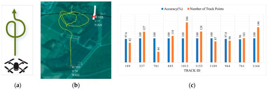
Figure 22.
Real-time classification results: (a) planned flight path; (b) real-time results; (c) statistical results.
In Figure 22a, the planned flight path is shown, starting with a straight flight followed by a circular trajectory. Figure 22b presents the real-time display results, and Figure 22c shows the accuracy and number of track points statistics after 10 flights. From the statistical chart, it can be observed that the real-time recognition accuracy for the drone is over 96% for all flights.
6. Conclusions
The concept of the LAE emphasizes the importance of radar as a critical tool for dynamic target detection. Ubiquitous radar, with its advantage of effectively detecting LSS targets in the cluttered urban environment, is particularly well-suited for applications in the LAE. This paper proposes a real-time classification process based on sliding window Doppler data, designed to meet the requirement for real-time classification (i.e., completing target classification using limited data as the trajectory extends frame by frame) and leveraging the high-resolution Doppler spectrum provided by the ubiquitous radar. Based on this process, a parallel multi-channel network using 1D ResNet-SE for target classification is designed. The network employs multiple channels to extract features from one-dimensional Doppler data within the window and uses an MLP for feature fusion. The incorporation of the 1D SE network further enhances the classification accuracy for drone targets, which are of significant concern in the LAE. Ultimately, the 1D ResNet-SE-MLP multi-channel parallel network achieved an overall classification accuracy of 99.58%, with the accuracy for drones reaching 99.44%. The experimental results demonstrate that the proposed classification process and multi-channel network perform well and can be effectively integrated into the real-time classification tasks of ubiquitous radar systems.
Author Contributions
Conceptualization, Q.S. and Z.D.; methodology, Y.Z.; software, Q.S.; validation, Q.S. and Y.Z.; formal analysis, Q.S.; investigation, Q.S.; resources, Y.Z.; data curation, Q.S.; writing—original draft preparation, Q.S.; writing—review and editing, Q.S., X.Z., X.C., Z.D., and Y.Z.; visualization, Q.S., S.H., X.Z., and W.L.; supervision, Y.Z.; project administration, Y.Z.; funding acquisition, Y.Z. All authors have read and agreed to the published version of the manuscript.
Funding
This research was funded by the National Natural Science Foundation of China under Grant U2133216 and the Science and Technology Planning Project of Key Laboratory of Advanced IntelliSense Technology, Guangdong Science and Technology Department under Grant 2023B1212060024.
Data Availability Statement
The datasets presented in this article are not readily available because they are generated from proprietary equipment and are subject to commercial confidentiality.
Conflicts of Interest
The authors declare no conflicts of interest.
References
- Zhang, H.; Wang, L.; Tian, T.; Yin, J. A Review of Unmanned Aerial Vehicle Low-Altitude Remote Sensing (UAV-LARS) Use in Agricultural Monitoring in China. Remote Sens. 2021, 13, 1221. [Google Scholar] [CrossRef]
- Björklund, S.; Johansson, T.; Petersson, H. Target Classification in Perimeter Protection with a Micro-Doppler Radar. In Proceedings of the 2016 17th International Radar Symposium (IRS), Krakow, Poland, 10–12 May 2016; pp. 1–5. [Google Scholar]
- Ślesicki, B.; Ślesicka, A. A New Method for Traffic Participant Recognition Using Doppler Radar Signature and Convolutional Neural Networks. Sensors 2024, 24, 3832. [Google Scholar] [CrossRef] [PubMed]
- Lee, U.-J.; Ahn, S.-J.; Choi, D.-Y.; Chin, S.-M.; Jang, D.-S. Airspace Designs and Operations for UAS Traffic Management at Low Altitude. Aerospace 2023, 10, 737. [Google Scholar] [CrossRef]
- Schneider, M.; Oestreicher, N.; Ehrat, T.; Loew, S. Rockfall Monitoring with a Doppler Radar on an Active Rockslide Complex in Brienz/Brinzauls (Switzerland). Nat. Hazards Earth Syst. Sci. 2023, 23, 3337–3354. [Google Scholar] [CrossRef]
- Reale, F.; Pugliese Carratelli, E.; Di Leo, A.; Dentale, F. Wave Orbital Velocity Effects on Radar Doppler Altimeter for Sea Monitoring. J. Mar. Sci. Eng. 2020, 8, 447. [Google Scholar] [CrossRef]
- Zhao, X.; Zhao, X.; Liu, Z.; Zhang, W. A Method to Track Moving Targets Using a Doppler Radar Based on Converted State Kalman Filtering. Electronics 2024, 13, 1415. [Google Scholar] [CrossRef]
- Tran, V.P.; Al-Jumaily, A.A.; Islam, S.M.S. Doppler Radar-Based Non-Contact Health Monitoring for Obstructive Sleep Apnea Diagnosis: A Comprehensive Review. Big Data Cogn. Comput. 2019, 3, 3. [Google Scholar] [CrossRef]
- Guo, R.; Zhang, Y.; Chen, Z. Design and Implementation of a Holographic Staring Radar for UAVs and Birds Surveillance. In Proceedings of the 2023 IEEE International Radar Conference (RADAR), Sydney, Australia, 6–10 November 2023; pp. 1–4. [Google Scholar]
- Jiang, W.; Wang, Y.; Li, Y.; Lin, Y.; Shen, W. Radar Target Characterization and Deep Learning in Radar Automatic Target Recognition: A Review. Remote Sens. 2023, 15, 3742. [Google Scholar] [CrossRef]
- Kiranyaz, S.; Avci, O.; Abdeljaber, O.; Ince, T.; Gabbouj, M.; Inman, D.J. 1D Convolutional Neural Networks and Applications: A Survey. Mech. Syst. Signal Process. 2021, 151, 107398. [Google Scholar] [CrossRef]
- Kiranyaz, S.; Ince, T.; Abdeljaber, O.; Avci, O.; Gabbouj, M. 1-D Convolutional Neural Networks for Signal Processing Applications. In Proceedings of the ICASSP 2019—2019 IEEE International Conference on Acoustics, Speech and Signal Processing (ICASSP), Brighton, Great Britain, 12–17 May 2019; pp. 8360–8364. [Google Scholar]
- Sung, Y.-H.; Park, S.-J.; Kim, D.-Y.; Kim, S. GPS Spoofing Detection Method for Small UAVs Using 1D Convolution Neural Network. Sensors 2022, 22, 9412. [Google Scholar] [CrossRef]
- Mohine, S.; Bansod, B.S.; Bhalla, R.; Basra, A. Acoustic Modality Based Hybrid Deep 1D CNN-BiLSTM Algorithm for Moving Vehicle Classification. IEEE Trans. Intell. Transp. Syst. 2022, 23, 16206–16216. [Google Scholar] [CrossRef]
- Yanik, M.E.; Rao, S. Radar-Based Multiple Target Classification in Complex Environments Using 1D-CNN Models. In Proceedings of the 2023 IEEE Radar Conference (RadarConf23), San Antonio, TX, USA, 1–5 May 2023; pp. 1–6. [Google Scholar]
- Kim, A.R.; Kim, H.S.; Kang, C.H.; Kim, S.Y. The Design of the 1D CNN–GRU Network Based on the RCS for Classification of Multiclass Missiles. Remote Sens. 2023, 15, 577. [Google Scholar] [CrossRef]
- Xiang, Q.; Wang, X.; Lai, J.; Song, Y.; Li, R.; Lei, L. Group-Fusion One-Dimensional Convolutional Neural Network for Ballistic Target High-Resolution Range Profile Recognition with Layer-Wise Auxiliary Classifiers. Int. J. Comput. Intell. Syst. 2023, 16. [Google Scholar] [CrossRef]
- Wang, X.; Li, R.; Wang, J.; Lei, L.; Song, Y. One-Dimension Hierarchical Local Receptive Fields Based Extreme Learning Machine for Radar Target HRRP Recognition. Neurocomputing 2020, 418, 314–325. [Google Scholar] [CrossRef]
- Deng, J.; Cheng, L.; Wang, Z. Attention-Based BiLSTM Fused CNN with Gating Mechanism Model for Chinese Long Text Classification. Comput. Speech Lang. 2021, 68, 101182. [Google Scholar] [CrossRef]
- Umer, M.; Imtiaz, Z.; Ahmad, M.; Nappi, M.; Medaglia, C.; Choi, G.S.; Mehmood, A. Impact of Convolutional Neural Network and FastText Embedding on Text Classification. Multimedia. Tools Appl. 2023, 82, 5569–5585. [Google Scholar] [CrossRef]
- Gupta, B.; Prakasam, P.; Velmurugan, T. Integrated BERT Embeddings, BiLSTM-BiGRU and 1-D CNN Model for Binary Sentiment Classification Analysis of Movie Reviews. Multimed. Tools Appl. 2022, 81, 33067–33086. [Google Scholar] [CrossRef]
- Nisha, N.N.; Podder, K.K.; Chowdhury, M.E.H.; Rabbani, M.; Wadud, M.S.I.; Al-Maadeed, S.; Mahmud, S.; Khandakar, A.; Zughaier, S.M. A Deep Learning Framework for the Detection of Abnormality in Cerebral Blood Flow Velocity Using Transcranial Doppler Ultrasound. Diagnostics 2023, 13, 2000. [Google Scholar] [CrossRef] [PubMed]
- Sun, Y.; Lo, F.P.-W.; Lo, B. EEG-Based User Identification System Using 1D-Convolutional Long Short-Term Memory Neural Networks. Expert Syst. Appl. 2019, 125, 259–267. [Google Scholar] [CrossRef]
- Moghadam, A.D.; Karami Mollaei, M.R.; Hassanzadeh, M. A Signal-Based One-Dimensional Convolutional Neural Network (SB 1D CNN) Model for Seizure Prediction. Circuits Syst. Signal Process. 2024, 43, 5211–5236. [Google Scholar] [CrossRef]
- Gong, Y.; Ma, Z.; Wang, M.; Deng, X.; Jiang, W. A New Multi-Sensor Fusion Target Recognition Method Based on Complementarity Analysis and Neutrosophic Set. Symmetry 2020, 12, 1435. [Google Scholar] [CrossRef]
- He, K.; Zhang, X.; Ren, S.; Sun, J. Deep Residual Learning for Image Recognition. In Proceedings of the 2016 IEEE Conference on Computer Vision and Pattern Recognition (CVPR), Las Vegas, NV, USA, 27–30 June 2016; pp. 770–778. [Google Scholar]
- Hu, J.; Shen, L.; Sun, G. Squeeze-and-Excitation Networks. In Proceedings of the 2018 IEEE/CVF Conference on Computer Vision and Pattern Recognition, Salt Lake City, UT, USA, 18–22 June 2018; pp. 7132–7141. [Google Scholar]
- Yang, C.; Yang, W.; Qiu, X.; Zhang, W.; Lu, Z.; Jiang, W. Cognitive Radar Waveform Design Method under the Joint Constraints of Transmit Energy and Spectrum Bandwidth. Remote Sens. 2023, 15, 5187. [Google Scholar] [CrossRef]
- Zheng, Z.; Zhang, Y.; Peng, X.; Xie, H.; Chen, J.; Mo, J.; Sui, Y. MIMO Radar Waveform Design for Multipath Exploitation Using Deep Learning. Remote Sens. 2023, 15, 2747. [Google Scholar] [CrossRef]
- Chen, H.; Ming, F.; Li, L.; Liu, G. Elevation Multi-Channel Imbalance Calibration Method of Digital Beamforming Synthetic Aperture Radar. Remote Sens. 2022, 14, 4350. [Google Scholar] [CrossRef]
- Gaudio, L.; Kobayashi, M.; Caire, G.; Colavolpe, G. Hybrid Digital-Analog Beamforming and MIMO Radar with OTFS Modulation. arXiv 2020, arXiv:2009.08785. [Google Scholar]
- Hochreiter, S.; Schmidhuber, J. Long Short-Term Memory. Neural Comput. 1997, 9, 1735–1780. [Google Scholar] [CrossRef]
- Woo, S.; Park, J.; Lee, J.-Y.; Kweon, I.S. CBAM: Convolutional Block Attention Module. In Proceedings of the European Conference on Computer Vision (ECCV), Munich, Germany, 8–14 September 2018; volume 11211. pp. 3–19. [Google Scholar] [CrossRef]


Disclaimer/Publisher’s Note: The statements, opinions and data contained in all publications are solely those of the individual author(s) and contributor(s) and not of MDPI and/or the editor(s). MDPI and/or the editor(s) disclaim responsibility for any injury to people or property resulting from any ideas, methods, instructions or products referred to in the content. |
© 2024 by the authors. Licensee MDPI, Basel, Switzerland. This article is an open access article distributed under the terms and conditions of the Creative Commons Attribution (CC BY) license (https://creativecommons.org/licenses/by/4.0/).