Attribution of Vegetation Dynamics in the Yellow River Water Conservation Area Based on the Deep ConvLSTM Model

Abstract

Climate change and human activities have significantly impacted the long-term growth of vegetation, thereby altering the ecosystem’s response mechanisms. The Yellow River Water Conservation Area (YRWCA) is a critical ecological functional zone in China. Since 1982, the vegetation in the YRWCA has changed significantly, and the primary drivers of vegetation which changed before and after 2000 were identified as climate change and human activities, respectively. However, the extent to which different drivers contribute to the vegetation dynamics of the YRWCA remains uncertain. In this study, we introduced a modified deep Convolutional Long Short-Term Memory (ConvLSTM) model to quantify the contributions of climate change and human activities to vegetation change while considering the spatiotemporal heterogeneity. We identified areas with minimal human activity before 2000 using the residual trend method, and used the regional data from these areas to train the model. Subsequently, we applied the trained deep ConvLSTM model to perform an attribution analysis after 2000. The results show that the deep ConvLSTM effectively captures the impacts of climate change on vegetation growth and outperforms the widely used Random Forest model (RF). Despite the fact that the input data of RF were optimized, ConvLSTM still distinctly outperformed RF, achieving R², MAE, and RMSE values of 0.99, 0.013, and 0.018, respectively, compared to RF’s corresponding values of 0.94, 0.038, and 0.045. Since 2000, the regional normalized difference vegetation index (NDVI) has shown a broad increasing trend, particularly in dryland, primarily induced by human activities from 2006 to 2015. Furthermore, an analysis of changes in regional land use, particularly in drylands, revealed that the highest magnitude of conversion of farmland back to forest or grass was recorded from 2000 to 2005. However, the most significant contributions from human activities occurred from 2006 to 2015, indicating a time lag in vegetation recovery from these ecological programs. The attribution results provide valuable insights for the implementation of ecological programs, and the introduced deep ConvLSTM proves the suitability of deep learning models that capture spatiotemporal features in vegetation growth simulations, allowing for broader applications.

1. Introduction

Ecological restoration practices based on scientific evidence and proper planning and management practices are crucial for the protection and regeneration of terrestrial ecosystems [1,2]. China is a leader in afforestation [3,4], benefiting from government-financed ecological programs implemented within the country to address ecosystem degradation, including the Natural Forest Conservation Program (NFCP), the Grain to Green Program (GTGP), and the Three-North Shelterbelt Program (TSP), which have significantly enhanced ecosystem services [5,6]. The Yellow River Water Conservation Area (YRWCA), designated for ecological services, accounting for 38.3% of the Yellow River basin area and 84.1% of its natural runoff, has undergone severe climate changes and human activities (e.g., over-farming and ecological engineering) over recent decades [7]. Water conservation is considered a crucial ecological service function [8], and ecological programs have been implemented in the YRWCA to enhance regional ecological services. As the largest land retirement program globally in terms of its spatial extent, magnitude of payments, and duration, initiated in 1999, the GTGP [9] includes the YRWCA, which encompasses provinces such as Sichuan, Gansu, and Shaanxi, where the GTGP was initially pilot-tested. Since its implementation, the program has significantly promoted ecological restoration, including the greening of regional vegetation [6], resulting in notable variations in vegetation dynamics and vegetation influencing factors around the year 2000, with human activities playing an important role in the post-2000 era. In addition, climate change has significantly impacted this region [10], which has affected vegetation growth and ecosystem stability. Increasing temperatures and shifting precipitation patterns have led to changes to the vegetation growing seasons and water availability, further complicating the ecological dynamics of the YRWCA [7]. The climatic changes, in conjunction with human activities, underscore the complexity of managing and restoring ecosystems in the face of multiple, interacting environmental conditions.

Climate change and human activities lead to the widespread transformation and depletion of ecosystems [11] and are the main drivers affecting ecosystem services. Separating the impacts of climate change and human activities on ecosystem dynamics is of significant importance [12]. Process-based ecosystem models [13] and statistical methods [14,15] have been used to quantify their contributions, and the results of these attributions are of significant importance for the assessment and development of regional ecosystems [16]. However, the extent to which different drivers contribute to the vegetation dynamics of the YRWCA remains uncertain.

Vegetation is a critical component of terrestrial ecosystems, playing an important role in the carbon and nitrogen cycles and energy flows between the land and atmosphere [17,18]. Vegetation plays an important role in ecological services such as water conservation, soil conservation, and flood and drought mitigation [19]. As a key factor representing ecological restoration, the impact of ecological programs implemented at the YRWCA on vegetation remains unclear. The residual trend method is a fundamental widespread approach using statistical methods for attribution [20], which can effectively separate the impact of climate change and human activities on vegetation dynamics. This method entails regressing vegetation against climate factors, with the trend of the regression results over several years representing the impact of climate change [21]. The trend of the difference between the actual values and the regression values is considered to reflect the impact of human activities. Temperature, precipitation, and solar radiation are considered the three main factors influencing vegetation growth [22,23,24], which are always frequently empirically represented climate factors in regression. Additionally, considering the time-lag and cumulative effects of climate factors on vegetation [23,25], accounting for the climate factors from previous months, can better express the impact of the climate on vegetation when using statistical analysis.

The residual trend method can separate multi-year outcomes [20], whereas it cannot effectively distinguish between the contributions of climate change and human activities to vegetation growth over shorter time periods. The statistical forecasting of vegetation variations and scenario simulations using process-based ecosystem models are different approaches, but they are compatible [26]. With the advancement of machine learning models, the prediction of vegetation indices has evolved from traditional methods such as an Auto-Regressive Integrated Moving Average (ARIMA) [27] and boosted regression trees [28] to the use of complex neural networks [29], resulting in an improved predictive performance. Current research shows that process-based ecosystem models excel in comprehensive simulations and fundamental physical mechanisms [30]. However, they still exhibit biases over shorter time scales in certain instances [31]. This study explores the application of the novel deep learning method to assess the impact of various factors on vegetation changes across different time periods.

To study the response characteristics of vegetation growth to climate and surface factors, we introduced a modified deep Convolutional Long Short-Term Memory (ConvLSTM) model to construct a model for predicting vegetation growth. Originally proposed for real-time precipitation forecasting [32], ConvLSTM has been widely applied in various fields. In the field of the environment, ref. [33] proposed a PM2.5 prediction model based on ConvLSTM, which effectively captures spatiotemporal features and improves long-term trend predictions. For ENSO forecasting, ref. [34] presented a modified ConvLSTM model that captures spatiotemporal dependencies in sea-surface temperature data, significantly enhancing the long-term prediction accuracy. In ecology, ref. [35] explored deep learning models, particularly ConvLSTM, to forecast vegetation dynamics in open ecosystems, demonstrating that the mean winter precipitation significantly improves the prediction accuracy. The suitability of the ConvLSTM model for vegetation prediction is high theoretically because it can capture the time-lag and cumulative effects presented in vegetation [23,36], as well as spatial patterns [37]. To the best of our knowledge, the application of ConvLSTM in predicting vegetation growth and disentangling the effects of climate change and human activities is rare.

To validate the simulation performance, we used the Random Forest (RF) model for comparison. RF [38] is a basic machine learning method known for its simple structure and good performance, widely used across various fields. For instance, ref. [39] optimized a RF to predict the corn yield. A Support Vector Machine and RF were used [40] to analyze the vegetation dynamics and greenness in China’s ecological restoration zones from 1990 to 2015, revealing that human activities contributed by over 100% to NDVI increases. Considering that traditional statistical models for studying vegetation responses to climate change often fail to adequately account for the influence of various climatic factors, static terrestrial factors, as well as spatial and temporal heterogeneity, we introduced a modified deep ConvLSTM model to quantify the contributions of climate change and human activities to vegetation changes while considering the aforementioned factors.

In light of the complex impacts of regional climate change and human activities on vegetation dynamics around 2000 in the YRWCA, we investigated the applicability of both deep ConvLSTM and RFs for predicting vegetation growth, and applied them to attribute the impacts of climate change and human activities on vegetation growth. Our study includes: (1) Analyzing the multi-year dynamics of regional NDVI, climate factors, and human activities, and obtaining the time-lag characteristics of vegetation in response to different climate factors. (2) Using the residual trend method with climate factors considering the time-lag and cumulative effects to separate the differences in the impact of regional climate change and human activities before and after 2000. (3) Constructing a deep ConvLSTM model and comparing its performance with the RF model. (4) Applying the deep ConvLSTM to separate the contributions of climate change and human activities in the years following 2000 and to assess the effects of ecological programs implemented in the region.

2. Materials and Methods

2.1. Study Area

The Yellow River Water Conservation Area, designated for ecological services, contains much of the river’s natural runoff. Located in Figure 1, it encompasses basins above Lanzhou on the main Yellow River, the Wei River (excluding the Jing and Bei-Luo Rivers), and the Yi-Luo River basins (hereafter referred to as A, B, and C, respectively). It serves as a primary source of water for the Yellow River basin, covering six provinces: Qinghai, Gansu, Ningxia, Sichuan, Shaanxi, and Henan. Geographically, according to the topography in Figure 1, area A is characterized by plateaus and mountains, while areas B and C are predominantly plains, with A and B separated by China’s first- and second-order terrain boundary lines; the northern part of A is semi-arid, while other areas are semi-humid. The western part of area B encompasses the upper reaches of the Wei River, and the eastern lower part reaches includes the Guanzhong Plain; the south of areas B and C covers the Qinling Mountains. The long-term mean precipitation, temperature, and radiation data for the YRWCA are shown in the spatial distribution map in Figure S1 of the Supplementary Materials.

2.2. Data

2.2.1. NDVI Data

The NDVI is a recognized indicator of vegetation productivity with extensive time series and data availability from different remote sensing products [41] and is often used to study regional vegetation changes and their relationships with environmental factors [42]. We use the NDVI as the indicator of vegetation growth.

The NDVI used here is obtained from the GIMMS NDVI 3g.v1 [43]. This dataset spans from July 1981 to December 2015 on a global scale, with a 15-day temporal resolution and a spatial resolution of 1/12°. The product created by the National Aeronautics and Space Administration (NASA) using images from the Advanced Very-High-Resolution Radiometer (AVHRR) on-board the National Oceanic and Atmospheric Administration (NOAA) series satellites. The GIMMS NDVI3g.v1 dataset underwent radiometric calibration, atmospheric correction, and coordinate transformation. The data had a high signal-to-noise ratio.

To ensure temporal and spatial resolution consistency for our study, NDVI data were resampled by bilinear interpolation and processed using the Maximum Value Composite (MVC) method to a spatial resolution of 0.1° on a monthly scale [44]. Vegetation indices in the growing season can better reflect vegetation dynamics. There are multiple methodologies for defining the start and end of the vegetation growing season [45]; here, the vegetation growing season is simply empirically defined using multi-year monthly average temperatures above 0 °C and multi-year monthly NDVI values above 0.2 [46], while other data are masked. The spatial results of the calculated growing season, as shown in the spatial distribution map in Figure S2, indicate that the duration of the growing season generally increases from west to east. This change is correlated with variations in the topography, climate, and vegetation.

2.2.2. Climate Data

Climate factor data are derived from the European Center for Medium-Range Weather Forecasts (ECMWF) Reanalysis 5-Land (ERA5-Land) dataset [47]. ERA5 is the ECMWF’s fifth-generation global atmospheric reanalysis dataset, covering from January 1950 to the present. Compared to ERA5, ERA5-Land provides several decades of land variables at a higher resolution at about 0.1°. ERA5-Land data are widely used in research due to their effectiveness on a monthly scale.

The monthly average temperature (t2m), maximum temperature (tmax), minimum temperature (tmin), total precipitation (tp), radiation (ssrd), dew point temperature (d2m), zonal wind (u10), meridional wind (v10), and pressure (sp) were selected as climate factors due to their proven direct or indirect impacts on vegetation growth [13,48]. Climate factors were also resampled to the same spatiotemporal resolution as the NDVI.

2.2.3. Land Use Data

Land use data are derived from the China Land Use [49], which is a remote sensing monitoring database and covers seven periods: the late 1980s, 1990, 1995, 2000, 2005, 2010, and 2015. Data production is primarily based on Landsat TM/ETM remote sensing images, created through manual visual interpretation. Data land use types include six primary categories: cropland, forestland, grassland, water bodies, residential areas, and unused land, along with 25 secondary types.

The land use data are maintained at a spatial resolution of 1 km for calculating the proportions of different land types at a 0.1° resolution. Within the 0.1° range, areas where the predominant land cover type exceeds 1/3 are assigned the corresponding land use type (points with less than 1/3 coverage are masked) in the pixels. For the study of natural vegetation dynamics, irrigated fields, water bodies, residential areas, and unused land (except wetlands) are masked. Residual vegetation types are then classified into 6 distinct categories, including dryland, forest, shrubland, meadow, grassland, and wetland. To analyse the dynamics in different vegetation classifications, the 2015 results are used as the distribution of vegetation types in the region.

2.2.4. Topographic and Soil Data

Digital Elevation Model (DEM) data for China [49] are derived from the Shuttle Radar Topography Mission (SRTM) conducted by the US Space Shuttle Endeavour. We used the resampled data with a 1 km resolution for our analysis. The soil data are derived from the Chinese Soil Texture Spatial Distribution dataset and are classified according to the proportion of sand, silt, and clay particles.

Using the ArcGIS 10.2 toolkit, DEM and soil data are aggregated and resampled to derive 0.1° spatial resolution surface elevation (dem), slope, aspect, elevation coefficient of variation (ecv), and the percent of sand, silt, and clay.

2.3. Method

2.3.1. Time-Lag Weighted Climate Factors

Given the time-lag and the cumulative effects of climate factors on vegetation, the use of time-lag weighted climate factors to analyse vegetation dynamics allows a more accurate reflection of the impact of climate on vegetation [23]. The current study empirically shows that vegetation indices were generally correlated with climate factors in the last four months, including the present month. Referring to [25], the method in our study to quantify the time-lag of individual climate factors is transformed into an optimization problem:

$$\begin{array}{l}{\max }_{la{g}_0,la{g}_1,la{g}_2,la{g}_3}\\ |corr(la{g}_0\cdot x_0+la{g}_1\cdot x_1+la{g}_2\cdot x_2+la{g}_3\cdot x_3,y)|\end{array}$$

(1)

$$\begin{array}{ll}s.t.& la{g}_0,la{g}_1,la{g}_2,la{g}_3\ge 0,\\ & la{g}_0+la{g}_1+la{g}_2+la{g}_3=1\end{array}$$

(2)

where $x_0,x_1,x_2,x_3$ denote the values of climate factors in the current and the previous 1, 2, and 3 months, respectively; $y$ denotes the NDVI of the current month; $corr$ denotes the Pearson correlation value; and $la{g}_0,la{g}_1,la{g}_2,la{g}_3$ are the time-lag factors to be optimized under constraint (2). Subsequently, the optimized results are used to calculate the time-lag weighted factor by the following calculations:

$$x=la{g}_0\cdot x_0+la{g}_1\cdot x_1+la{g}_2\cdot x_2+la{g}_3\cdot x_3$$

(3)

where $x$ is the climate factor; $x_0,x_1,x_2,x_3$ are the climate factor for the current month and the previous 1, 2, and 3 months; and $la{g}_x$ is the previously computed time-lag weight. Meanwhile, we could obtain the average time-lag of different climate factors by the obtained weighted factors through the following equation:

$$T=la{g}_0\cdot 0+la{g}_1\cdot 1+la{g}_2\cdot 2+la{g}_3\cdot 3$$

(4)

where $T$ indicates the average time-lag of various climate factors; integers 0, 1, 2, and 3 mean the current and previous months; and $la{g}_x$ is as mentioned above. Pearson correlations [50] are calculated between various weighted factors and NDVI as the following:

$$r={\displaystyle \frac{{\displaystyle \sum _{i=1}^n(}{X}_i-\overline{X})(Y_i-\overline{Y})}{\sqrt{{\displaystyle \sum _{i=1}^n(}{X}_i-\overline{X}{)}^2}\sqrt{{\displaystyle \sum _{i=1}^n(}{Y}_i-\overline{Y}{)}^2}}}$$

(5)

where $r$ is the Pearson correlation value; $n$ is the whole number of months in the growing season; $X_i$ and $\overline{X}$ are the weighted climate factor in a certain month value and multi-year average, respectively; $Y_i$ and $\overline{Y}$ represent the NDVI at the same scale. A T-test is used for the Pearson correlation significance test.

2.3.2. Residual Trend Method

The residual trend method [51] is calculated as:

$$NDV{I}_{cc}=a\times T+b\times P+c\times S+d$$

(6)

$$NDV{I}_{hh}=NDV{I}_{obs}-NDV{I}_{cc}$$

(7)

where $NDV{I}_{cc}$ denotes the NDVI of the multiple linear regression, characterizing the impact of climate change; $T,P,S$ are the time-lag weighted temperature, precipitation, and solar radiation, respectively; $a,b,c,d$ are the regression coefficients and the residual of the temperature, precipitation, and radiation in the linear regression, respectively; $NDV{I}_{hh}$ characterizes the impact of human activities; and $NDV{I}_{obs}$ is the actual observed value of the NDVI. The reason for utilizing temperature, precipitation, and radiation as regression independent variables is that they have been empirically demonstrated to be the crucial climate factors influencing vegetation growth [52]. Linear trends [53] were calculated for the obtained $NDV{I}_{cc}$ and $NDV{I}_{hh}$:

$$S={\displaystyle \frac{n{\displaystyle \sum _{i=1}^{n}i}\times N_i-{\displaystyle \sum _{i=1}^{n}i}{\displaystyle \sum _{i=1}^n{N}_i}}{n{\displaystyle \sum _{i=1}^n{i}^2}-{\left({\displaystyle \sum _{i=1}^{n}i}\right)}^2}}$$

(8)

where $S$ is the calculated trend; $n$ is the number of years of calculation; $N_i$ is the value of the variable in different years; and $i$ is the ordinal number of different years. $S>0$ indicates an upward trend. Linear trends were also calculated in the multi-year NDVI and different climate factors. The F-test was then performed on the trend calculation results.

2.3.3. ConvLSTM and RF

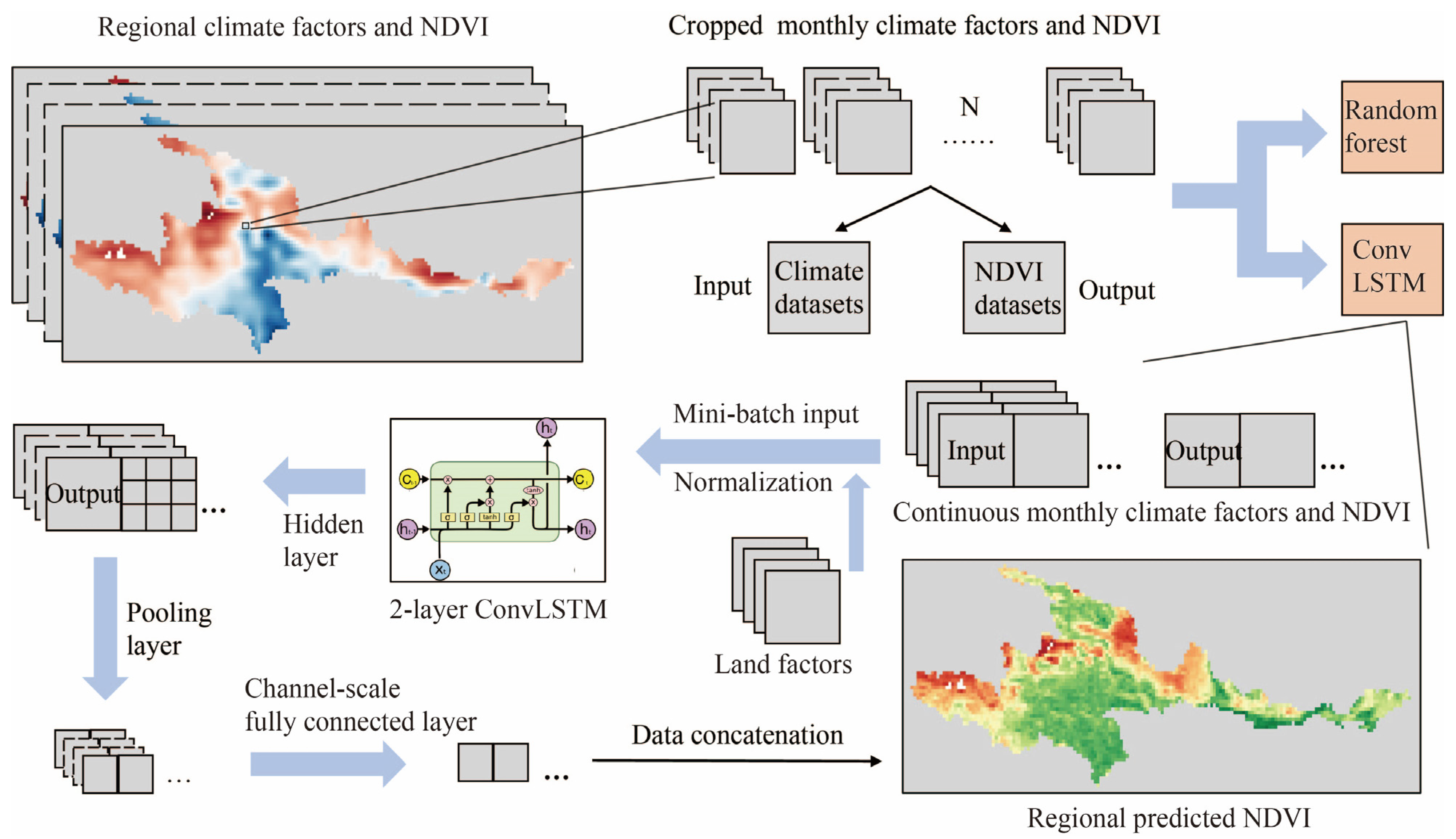
ConvLSTM is a hybrid model comprising a convolutional network and a LSTM model [32]. Given that vegetation growth responds to the climate with a time-lag and cumulative effects and exhibits spatial correlations, we introduced the deep ConvLSTM model to capture these characteristics. For the prediction of the NDVI, the model takes climate factors and certain terrestrial variables during the growing period as the input and the NDVI as the output. To increase the amount of data and model applicability, the specific structure of the model application is shown in Figure 2.

In contrast to the normal ConvLSTM structure, the deep ConvLSTM in our study takes into account the static terrestrial factors, refer to [54]. We also added a pooling layer after the convolution layer, which takes into account the spatial influences. The final fully-connected layer characterizes the combined effects of the different factors on vegetation. In order to ensure adequate training data, a cropping scheme was utilized to process the raw spatial data.

To improve the applicability of the model, for the output of the NDVI for a given month, the input data are the climate factors and certain static terrestrial variables for the previous three months and the present month. The use of four months of climate data as the input to analyse the vegetation dynamics allows for a more accurate reflection of the impact of the climate on vegetation, which is due to the time-lag effect in the response of vegetation to the climate [23]. The time-lag effect exhibits a dependence on the time scale, not only at the interannual scale, but also at the seasonal and monthly scales [25,55,56]. On a monthly scale, a large number of the literature is obtained through linear regression and correlation analyses of vegetation and climate data from different data sources: there are differences in the time-lag of vegetation growth in response to different climate factors [42], and the time-lag on the monthly scale is mainly reflected within three months [25]. For example, [56] pointed out that there was a time-lag of about three months between the strongest change in temperature and the appearance of the trend-maximum change in the NDVI. The authors of [57] showed that for temperate grassland and temperate desert steppe, both the spring and autumn NDVI were positively correlated with the precipitation of the previous season (non-growing season and summer), which indicated that there was a time-lag of about three months. Furthermore, [41] observed that the NDVI in the U.S. Great Plains region had a time lag of two to four weeks for precipitation changes. These results reveal that the time-lag of vegetation is concentrated within four months. Using the spatial time-lag characteristics from Section 2.3.1, we found that the time-lag within the previous 3 months is a bit weaker. This explains why we chose to use four months of data as the input in this study.

RF is an integrated learning method [38], which is the basic machine learning method. An RF model with time-lag weighted factors as the input and the NDVI as the output is constructed to compare the performance of the deep ConvLSTM construction.

The input factors of both models include climate factors, t2m, tmax, tmin, tp, ssrd, d2m, u10, v10, and sp, and terrestrial factors, dem, slope, aspect, ecv, sand, silt, and clay, amounting to 16 variables. In order to ensure the model performance, both models were cross-validated 10-fold (see Text S1) to obtain the respective model optimal parameters. The constructed deep ConvLSTM model performs better than RF (see Section 3.4) and can better capture the impact of climate change on the NDVI. Given the structural characteristics of deep ConvLSTM and its excellent performance, this study employs deep ConvLSTM for subsequent attribution.

The constructed deep ConvLSTM model performs better than RF (see Section 3.4) and can better capture the impact of climate change on the NDVI. Given the structural characteristics of the deep ConvLSTM and its excellent performance, this study employs the ConvLSTM model for subsequent attribution.

The human activities in the YRWCA were intense after 2000. To better quantify the contribution of human activities to vegetation growth in the growing season after 2000, we utilized the results obtained before 2000 through the residual trend method. The data from grid points where human activities were deemed insignificant were then selected as the input for model training. The trained model is applied to post-2000 predictions to separate the contributions of climate change and human activities.

2.3.4. Attributional Analysis

The de-trended results [58] of all climate factors after 2000, alongside the actual climate factors, are used as inputs for the deep ConvLSTM model, and the corresponding NDVI values are subsequently calculated:

$$\begin{array}{l}NDV{I}_{all}=NDV{I}_{obs}-NDV{I}_{basep}\\ NDV{I}_c=NDV{I}_{truep}-NDV{I}_{basep}\\ NDV{I}_h=NDV{I}_{obs}-NDV{I}_{truep}\end{array}$$

(9)

where $NDV{I}_{basep}$ is the output using the de-trended climate factors as the input, which represents the unchanged baseline result of the climate factors; $NDV{I}_{obs}$ is the observed NDVI value; $NDV{I}_{truep}$ is the output using the actual climate factors as the input; and $NDV{I}_{all},NDV{I}_c,NDV{I}_h$ are the total change value of the NDVI, the change of the NDVI caused by climate change, and the change of the NDVI caused by human activities, respectively. Then, the ratios of changes in the NDVI to the baseline NDVI, associated with climate change and human activities, were calculated:

$$\begin{array}{l}NDV{I}_{RC}={\displaystyle \frac{NDV{I}_c}{\overline{NDV{I}_{basep}}}}\\ NDV{I}_{RH}={\displaystyle \frac{NDV{I}_h}{\overline{NDV{I}_{basep}}}}\end{array}$$

(10)

where $\overline{NDV{I}_{basep}}$ is the mean value of the baseline results after 2000; $NDV{I}_{RC}$ and $NDV{I}_{RH}$ are denoted as the climate-based ratio and human-based ratio, respectively.

2.3.5. Anthropogenic Magnitude

Referring to [59], the anthropogenic activities in our study are categorized into ecological restoration and over-farming. Areas converted from unused land or farmland into forest, grassland, or wetlands are classified as ecological restoration areas. Conversely, areas where unused land, forest, grassland, or wetlands have been converted into farmland are designated as over-farming areas. Based on this classification, data on anthropogenic activities for six periods were obtained and expressed as percentages in pixels. The anthropogenic magnitude is calculated based on the proportions of ecological restoration and over-farming areas at a 0.1° resolution:

$$A=R-O$$

(11)

where $A$ denotes the anthropogenic magnitude and $A>0$ indicates that the area is ecologically restored, and $R$ and $O$ denote ecological restoration and the over-farming area, respectively.

3. Results

3.1. Dynamics in NDVI and Environmental Factors

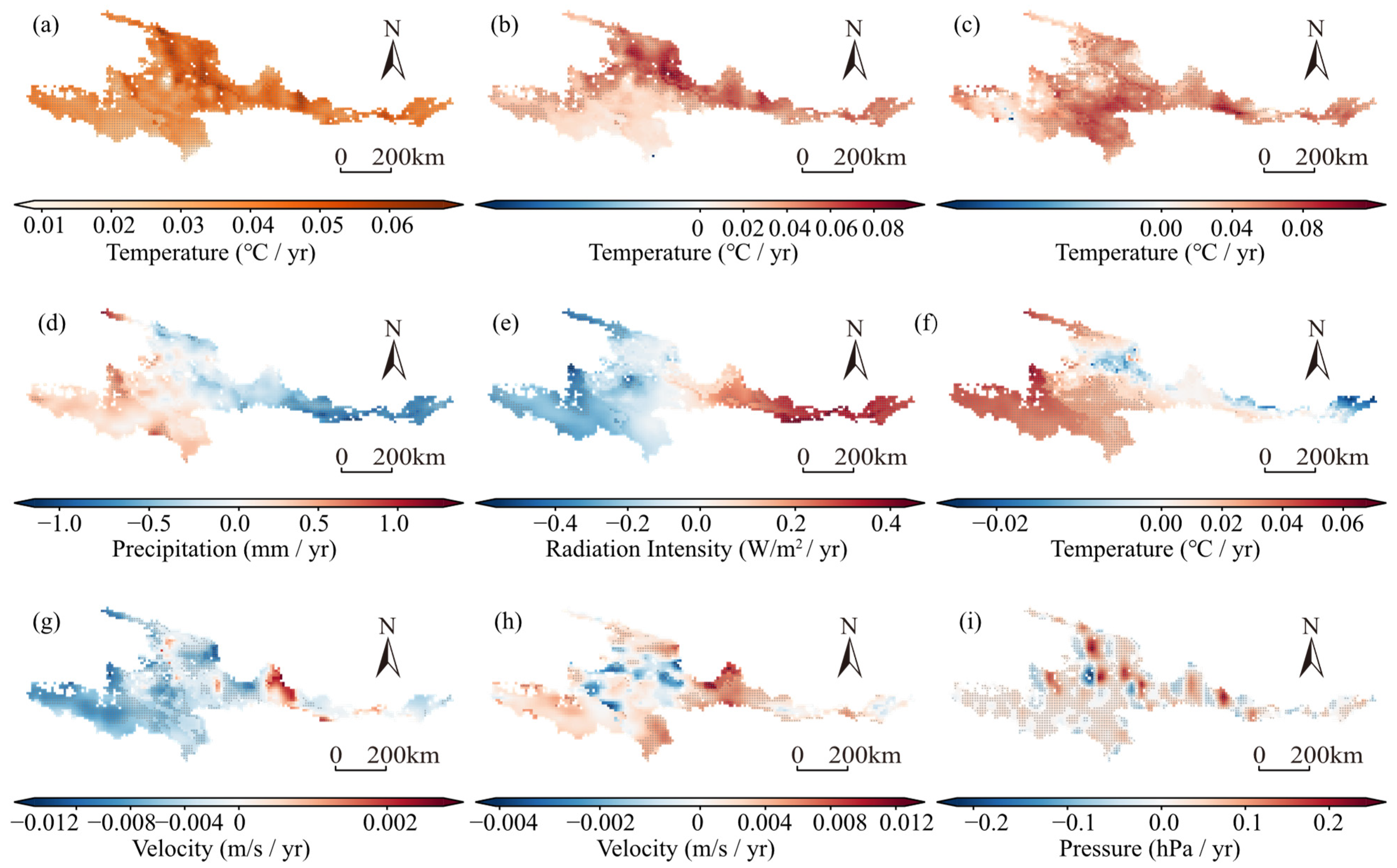
The type of natural vegetation is determined by climatic conditions [60], and there is a consistent relationship between the NDVI, vegetation type, and climatic conditions, as shown in Figure 3. For instance, meadows have more adequate precipitation conditions than grassland (refer to the spatial distribution maps in Figures S1 and S3). The vegetation in areas B and C is mainly composed of dryland, forest, and shrubland, while the western part of the YRWCA is dominated by meadow, grassland, and wetland. A lot of areas in the YRWCA have shown a significantly increasing trend of the NDVI over the years. Figure 4 and Figure 5 give the spatial distribution maps of climate factor changes during the growing season of vegetation and the intensity change of human activities, respectively. The NDVI shows the strongest growing trend in the upper Wei River, area C and northeast area A, which were also the areas with the highest levels of over-farming before 2000.

Different climate factors and human activities have also changed over the years. As shown in Figure 4, the regional temperature and humidity have shown a broadly increasing trend over the years, while precipitation and radiation show different trends over the eastern and western parts of the YRWCA, with more significant changes in regions B and C. Multi-year trends in climate factors such as precipitation, temperature, and radiation could significantly affect vegetation dynamics.

Figure 5 shows the intensity of human activities across three different time periods, highlighting the differences between the east and west of the YRWCA. In the west, there is less cultivated land, and a significant portion of unused land was converted to vegetation before 2000. In the east, there was extensive cultivated land and notable over-farming before 2000, followed by ecological restoration efforts after 2000. The implementation of ecological projects such as the GTGP after 2000 has significantly impacted human activities in the east, where the strongest NDVI growth trend is observed.

Different vegetation types in the YRWCA have different characteristics (see

Table 1. Characteristics of different vegetation types in the YRWCA.

	Area Proportion	NDVI Multi-Year Average	NDVI Multi-Year Trend	Significant Area	Growing Season Duration
Units	(%)		(yr−1·10−3)	(%)	(month)
Region		0.53	0.85	52.1	6.3
Dryland	17.1	0.43	1.59	80.6	9.0
Forest	6.2	0.64	1.18	71.0	8.8
Shrubland	2.7	0.63	0.58	41.7	6.3
Meadow	32.0	0.62	0.46	35.8	6.0
Grassland	40.9	0.46	0.81	50.5	4.9
Wetland	1.1	0.61	0.66	56.7	5.9

). Drylands and forestlands exhibit the strongest NDVI increasing trends, with rates of 0.00159 yr⁻¹ and 0.00118 yr⁻¹, respectively, while they also have the largest areas of significant change. Meadows have the lowest growth trend at 0.00046 yr⁻¹. We also assessed the impacts of human activities on different vegetation types (Table S1). The results show that drylands are the only vegetation type significantly affected by over-farming before 2000 and ecological restoration after 2000.

3.2. Response of Different Vegetation Types to Climate Factors

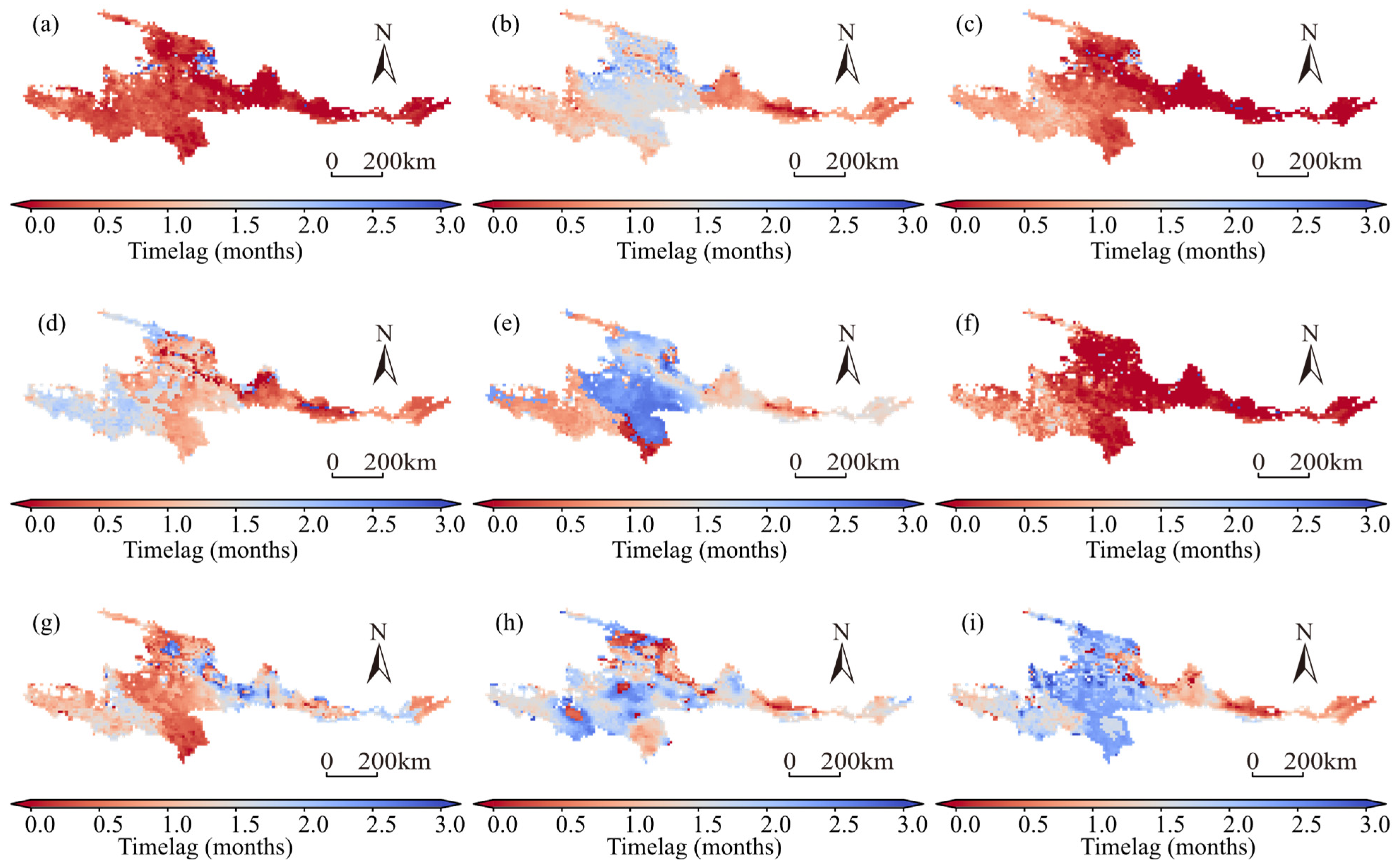
The spatial distribution of the mean time-lag of each climatic factor on vegetation was obtained using the calculated weights of different climate factors over the past four months (see Figure 6). The mean time-lag for different vegetation types is shown in

Table 2. Mean time-lag of various climate factors on different vegetation species.

	t2m	tmax	tmin	tp	ssrd	d2m	u10	v10	sp
Time-Lag	(month)
Region	0.28	1.22	0.44	1.09	1.58	0.30	1.08	1.53	1.67
Dryland	0.08	0.76	0.11	0.60	1.28	0.06	1.32	1.31	0.94
Forest	0.16	1.00	0.09	0.84	1.64	0.10	1.43	1.39	1.43
Shrubland	0.20	1.42	0.32	1.27	1.92	0.23	1.01	1.65	1.96
Meadow	0.23	1.36	0.45	1.16	1.82	0.27	0.85	1.64	2.01
Grassland	0.45	1.31	0.64	1.28	1.48	0.45	1.14	1.56	1.72
Wetland	0.17	1.47	0.32	1.15	2.06	0.16	0.49	1.29	1.82

. Wind speed and air pressure, which drive the flow of atmospheric matter and energy, exhibit a relatively high time-lag. Excluding wind speed and air pressure, for the whole region, vegetation has the highest time-lag for tmax, tp, and ssrd, each exceeding one month, while other factors have time-lags of less than one month. For drylands specifically, the time-lags for tmax, tp, and ssrd are the highest at 0.76, 0.60, and 1.60 months, respectively, with lower time-lags for other factors.

According to the correlation analysis results in

Table 3. Pearson correlation results of NDVI with each weighted climate factor for different vegetation types.

	t2m	tmax	tmin	tp	ssrd	d2m	u10	v10	sp
Region	0.81 *	0.78 *	0.77 *	0.65 *	0.32 *	0.80	−0.53 *	−0.23	0.33
Dryland	0.75 *	0.72	0.68 *	0.45 *	0.72	0.69	−0.22	0.29	−0.47
Forest	0.87 *	0.87 *	0.81	0.58	0.83 *	0.82	−0.34	0.32 *	−0.37
Shrubland	0.89 *	0.86 *	0.87 *	0.74	0.63 *	0.88 *	−0.64 *	−0.28	0.56 *
Meadow	0.88	0.83 *	0.85	0.75 *	0.37	0.88 *	−0.68	−0.44 *	0.63 *
Grassland	0.77	0.73	0.73 *	0.66 *	0.02	0.76	−0.56 *	−0.36 *	0.50 *
Wetland	0.88 *	0.85 *	0.87	0.79 *	0.39 *	0.88 *	−0.78 *	−0.66	0.78

“*” indicates that the test of significance is less than 0.05.

, the main factors affecting the NDVI for the entire study area are t2m, tmax, tmin, and d2m. For dryland and woodland, the key factors are t2m, tmax, tmin, ssrd, and d2m. In contrast, shrubs, grassland, meadows, and wetlands are primarily influenced by t2m, tmax, tmin, tp, and d2m. Wind speed and air pressure, being indirect influences, have lower impact values compared to other climate factors. However, their impact is more significant for shrublands, meadows, grasslands, and wetlands than for drylands and forests, which thrive in wetter conditions. These findings justify the use of the past four months of data as training inputs for the deep learning model.

The discrepancy in Pearson’s correlation outcomes for diverse vegetation types can be attributed to the fact that different vegetation growth has different hydrothermal conditions [61]. Furthermore, precipitation is adequate to ensure that moisture will not exert a controlling influence on vegetation growth [62]. In drier conditions, moisture becomes a limiting factor for vegetation [63]. Meanwhile, wind speed and air pressure affect vegetation growth indirectly, through their impact on evapotranspiration [64], particularly in sparsely vegetated areas. Consequently, the correlation for precipitation and wind speed is heightened in shrub, meadow, grassland, and wetland vegetation.

The analysis of the time-lag effect of each climatic factor on vegetation may have limitations because such a result does not take into account the covariance of different climate factors [65]. Therefore, this method tends to produce higher Pearson correlation values, as it seeks the optimal Pearson value. However, the results in Table 3 are still representative. For example, the NDVI of grassland and meadows grown in drier areas shows a high correlation with precipitation, as water is a limiting factor for the growth of these vegetations.

3.3. Residual Trend Analysis

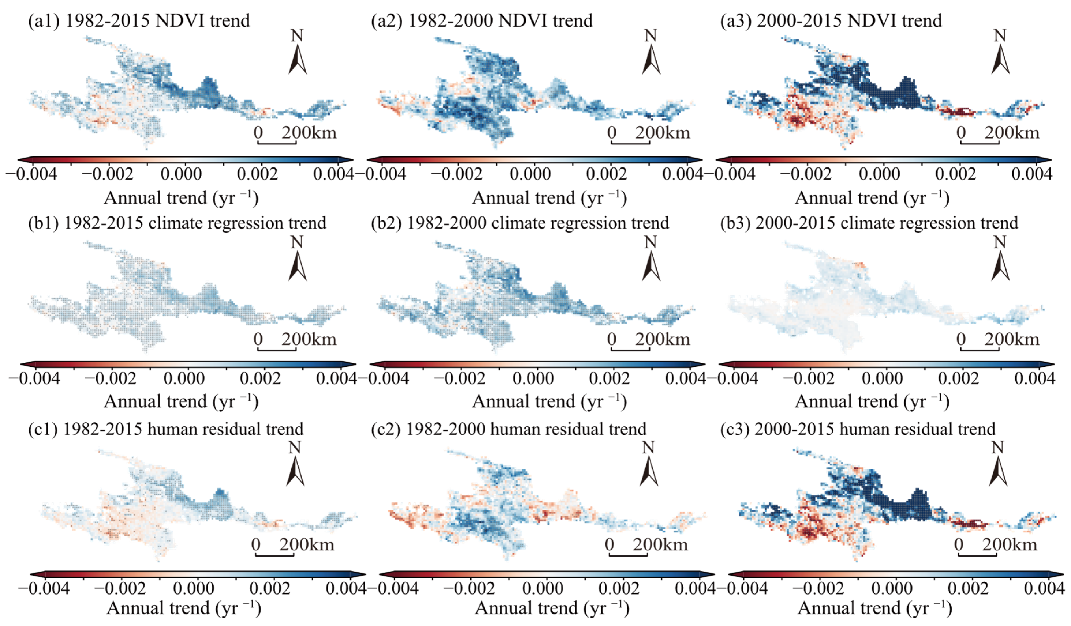
The implementation of ecological programs since 2000 has shifted the drivers of vegetation growth. Based on the results by the residual trend method (Figure 7), the NDVI trends in the Wei River basin, Yi-Luo River basin, and the northeast and western parts of Area A were driven by climate changes before 2000 and by human activities after 2000, while the growth trend in the southern part of Area A was driven by climate changes both before and after 2000. The declining vegetation trends in the Guanzhong Plain and the south-western part of area A are attributed to climate changes before 2000 and the suppressive effects of human activities after 2000.

In the plain areas, where dryland is the predominant land use, there was widespread over-farming before 2000 and ecological restoration afterward, corresponding to the changes in vegetation trends caused by human activities. The significant decrease in vegetation in the Guanzhong Plain was due to the detrimental impact of human activities on vegetation growth after 2000. The data in areas where human activities were not significant before 2000 were used as training data for the two machine learning models.

3.4. Contributions of Climate Change and Human Activities on NDVI Since 2000

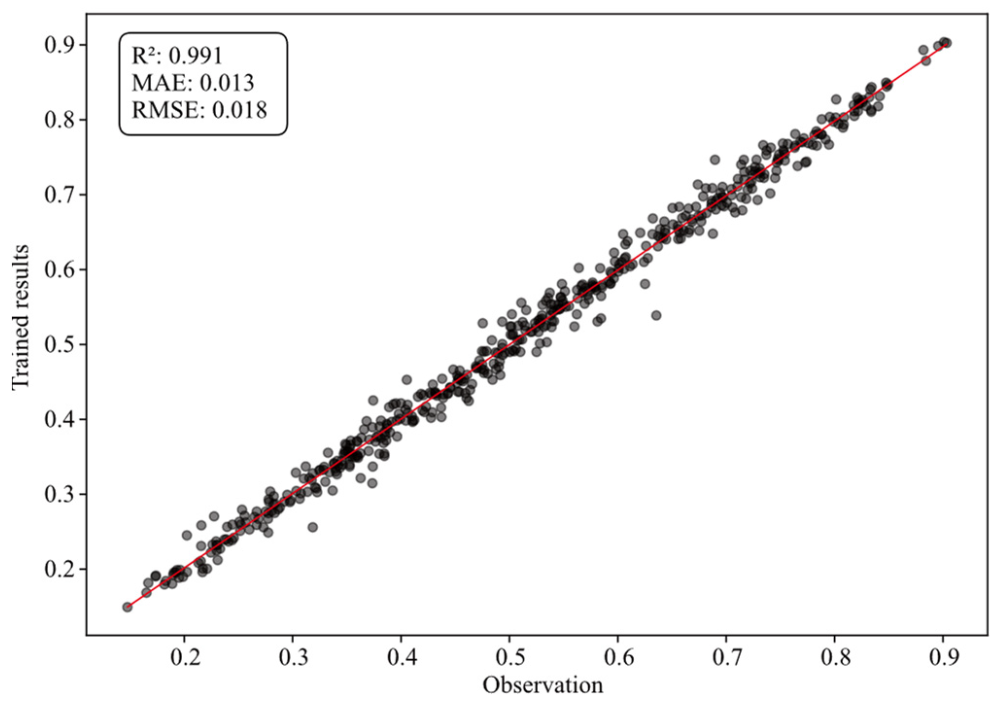
The ConvLSTM model performs very well in predicting the NDVI (Figure 8) and has a better performance than the widely used RF model (

Table 4. Comparison of the deep ConvLSTM and RF results based on three evaluation metrics.

Metrics		R2	MAE (10−3)	RMSE (10−3)
RF	training period	0.9860	16.3	22.1
	validation period	0.9430	33.7	44.7
Modified deep ConvLSTM	training period	0.9995	3.3	4.2
	validation period	0.9910	13.0	17.7

). The spatial trends of $NDV{I}_c$ and $NDV{I}_h$ show similarities (spatial distribution map in Figure S4) with the results in Figure 7(a3,b3,c3), demonstrating that the model captured the post-2000 vegetation trends influenced by climate change and human activities, indicating that the model can capture vegetation dynamics.

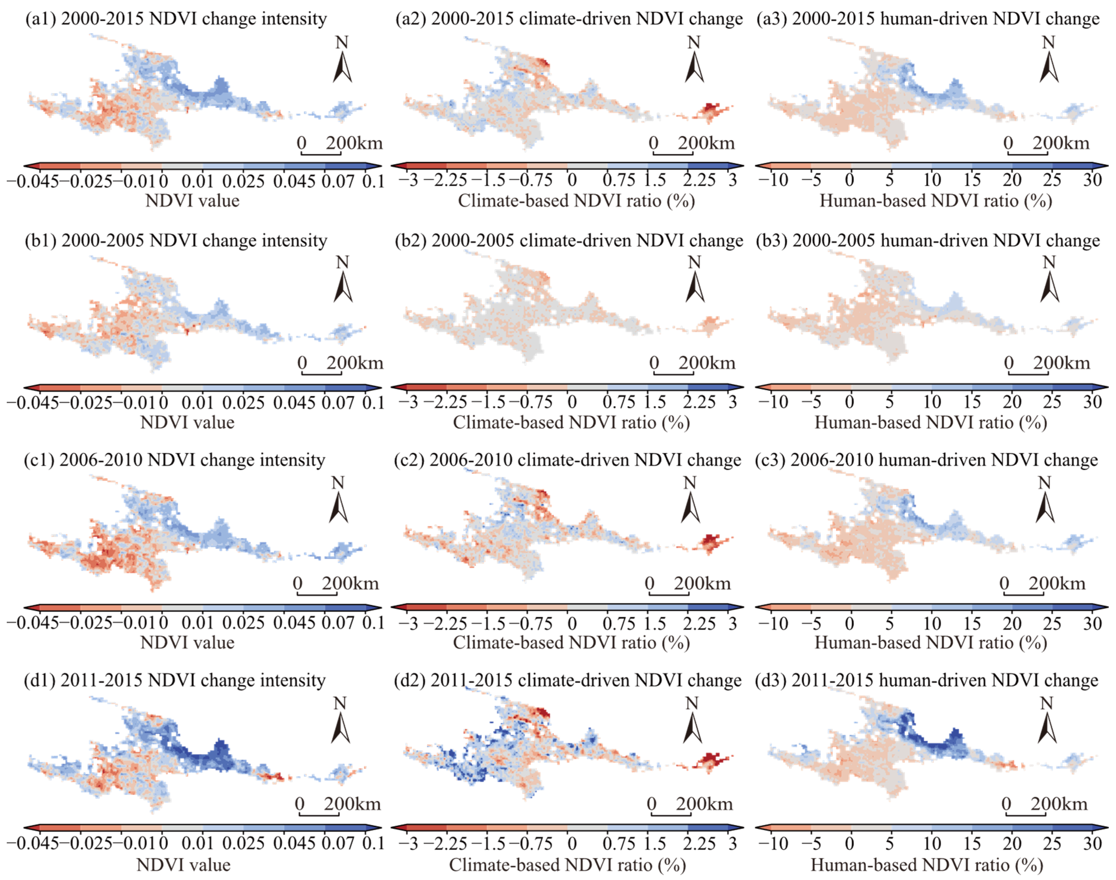
After 2000, the contribution of climate change on the NDVI in the study area is relatively weaker compared to the influence of human activities on the NDVI. Human activities exerted an increasing influence on the NDVI in the YRWCA over time (Figure 9). Spatial vegetation changes vary due to the different impacts of human activities and climate change. The NDVI in the Yi-Luo River basin exhibited an increasing change due to human activities from 2006 to 2015, despite climate change partially mitigating the intensity of human activities. In the Guanzhong Plain, the decreasing NDVI change from 2011 to 2015 was due to the increasing trend of human activities causing damage to vegetation. The increase in the NDVI in the upper-middle Wei River and the northeast and western parts of area A is due to the increasing promotion of human activities from 2006 to 2015. Conversely, the observed decline in the vegetation NDVI in the southwestern part of area A between 2006 and 2015 can be attributed to the suppressive effects of human activities on vegetation growth, which is consistent with the findings of [66,67]. During this period, grassland degradation was caused by human grazing, rodent infestations, and the spread of black-soil patches. However, climate change has mitigated the destructive intensity of human activities to some extent.

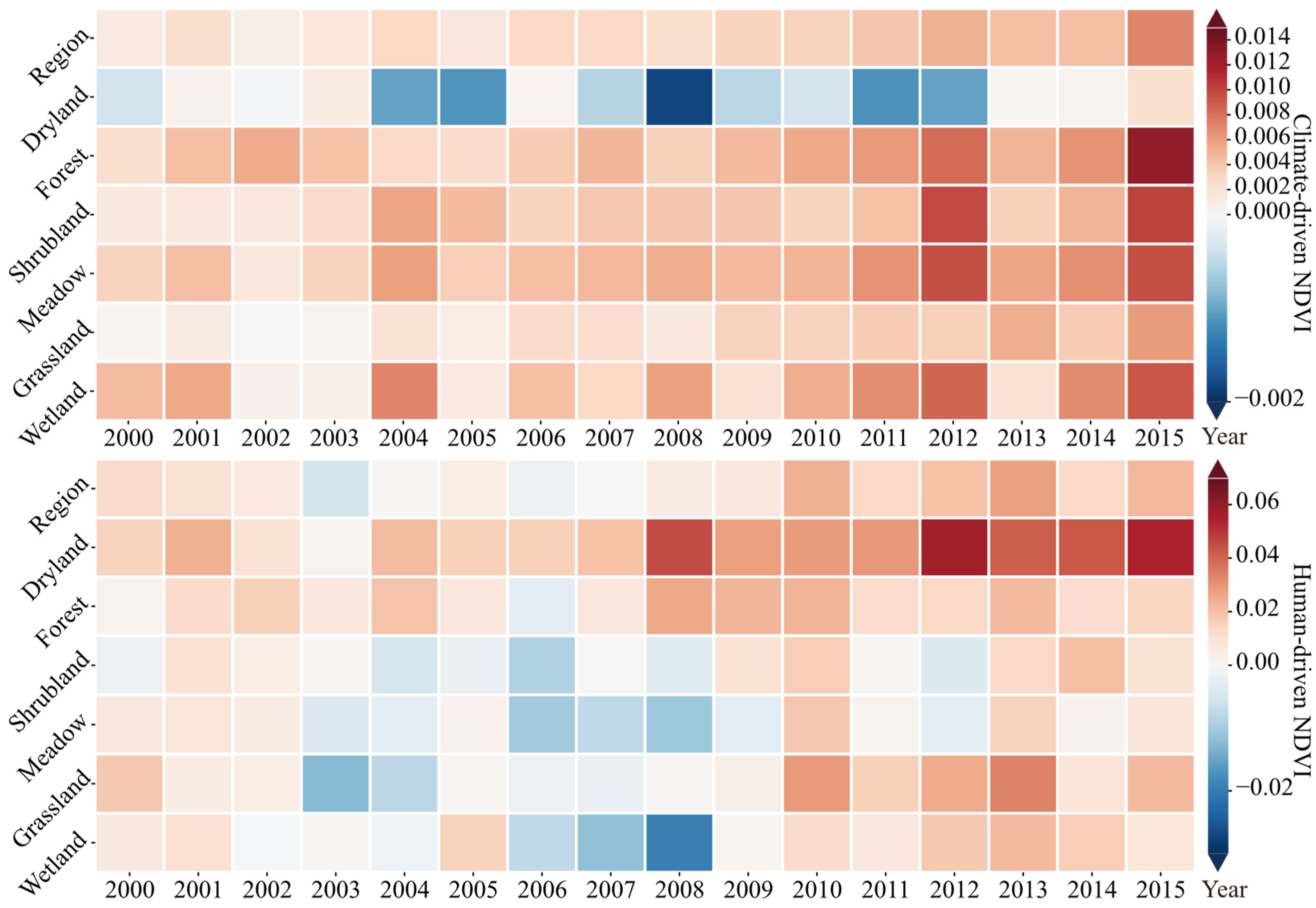
Overall, since the 2000s, human activities have generally enhanced the NDVI of different vegetation types (Figure 10). The results indicate that human activities had a negative contribution to the NDVI of shrub, grassland, meadow, and wetland types from 2003 to 2008. However, in subsequent years, human activities have again promoted vegetation growth.

3.5. Effects of Regional Ecological Programs

After 2000, the impact of climate change on vegetation growth is weaker than the impact of human activities, indicating that the main source of vegetation trends in the YRWCA is the implementation of human ecological programs. Post-2000, the vegetation trend, from strongest to weakest, is observed in drylands, grasslands, shrubs, forests, wetlands, and meadows. The NDVI growth trend in the study area post-2000 is 0.0015 yr⁻¹.

According to Figure 9, drylands received the strongest human activity contributions after 2000. Referring to the anthropogenic magnitude in different periods post-2000 (spatial distribution map in Figure S5), it is noted that extensive land was reforested from farmland between 2000 and 2005. From 2006 to 2015, the intensity of ecological restoration weakened, displaying a mixed pattern of restoration and over-farming. However, the human contribution on NDVI change, especially in drylands, has increased annually post-2000, indicating that the programs to convert farmland back to forest or grassland also have a delayed effect on ecosystem restoration. The results also demonstrate that the implementation of human ecological engineering in the YRWCA has shifted from initial farmland conversion to more optimized management schemes.

Despite the widespread implementation of regional ecological programs, the results from Figure 9 indicate that human activities, particularly in the south-western part of area A from 2000–2015, had a significant destructive impact on vegetation growth. However, the overall inhibitory effect of human activities on vegetation is insignificant, and this result was due to the combined influence of various factors, as the residual results do not solely represent the impact of human activities.

4. Discussion

Given that ConvLSTM is suitable for capturing spatiotemporal features [32], the deep ConvLSTM model is adept at capturing the impact of climate change on vegetation due to its ability to handle the time-lag and the cumulative effects of vegetation and the spatial patterns associated with vegetation. Although the performance of the RF is slightly inferior to that of deep ConvLSTM, it is still of a high standard because we use weighted climate factors for training. The achievement of this level of performance by the RF needs the implementation of complex data processing techniques and the undertaking of lengthy training periods (Table S2). For the inputs of models, we considered the last four months of data because the time-lag of vegetation has been empirically confirmed to be basically within four months [68] and also, according to Table 2 and Figure 6, it is valid to use four months of input data. Furthermore, the deep ConvLSTM model trained by cropping spatial data to expand the data volume shows superior training results due to its ability to accurately fit vegetation features.

In regard to the structure of the model illustrated in Figure 2, the inputs are climate factors and static terrestrial factors, while the output is the NDVI. Static terrestrial factors [69] are used as inputs because the same climatic conditions may have different effects on the vegetation in different areas [23] and, based on the importance of the different factors obtained by the RF (Figure S6), also proves that there is an effect of terrestrial factors on vegetation growth, especially dem. The superior training results obtained through this method have demonstrated the potential for the construction of deep learning models to be applied in a wider range of scenarios, including the simulation of future scenarios [70]. For example, ref. [45] demonstrated that machine learning models are more effective than process-based ecosystem models in capturing vegetation sensitivity. This advantage is also one of the reasons why deep learning models are used for the simulations in this paper.

Although the constructed model performs well, as evidenced by the training and validation results of vegetation dynamics changes before 2000 (Figure 8 and Table 4) and the prediction of NDVI trends driven by climate change and human activities after 2000 (spatial distribution map in Figure S4), it may also have model biases, which could lead to uncertainties in the simulation results. Furthermore, it is important to note that although the residual results are presented as human activities, the residuals may include factors that are not directly influenced by humans. For example, during the period from 2006 to 2010, the negative impact of residual results in the south-western part of area A may be attributed not only to potential model biases and human overgrazing, but also to other factors such as rodent infestations and the expansion of black-soil patches [71]. It can be observed that the degradation of vegetation in this area has improved in recent years.

Furthermore, ecological engineering might also have negative effects [72]. For instance, ref. [73] noted that large-scale tree planting by humans could exacerbate water shortages in semi-arid areas, thereby hindering vegetation restoration, which might partly explain the negative impacts of human activities in the south-western part of area A. Additionally, the negative impact on vegetation in the Guanzhong Plain stems from urbanization [74].

Climate differences are the dominant factors causing spatial heterogeneity in natural vegetation cover changes [75], indicating that ecological restoration has certain thresholds [16]. Therefore, ecological engineering might enable quicker restoration in drylands, while changes in other cover types are less pronounced. Meanwhile, due to the characteristics of different ecosystems, ecosystem restoration does have a certain time lag with the implementation of ecological programs [76], which is also consistent with the results we obtained in Section 3.5.

The results of the analysis of different vegetation types are somewhat uncertain due to the fact that the vegetation types are classified based on the largest area of vegetation per point in 2015. Consequently, the main vegetation types in some areas may have undergone significant changes. For instance, in the west of area A, where grassland is distributed, Figure 5 illustrates that a significant area underwent ecological restoration prior to 2000, largely due to the conversion of unused land to vegetation [77]. Additionally, Figure 7 indicates that human activities in the region were minimal before 2000, suggesting that this transformation was driven by climate change. Before 2000, climate change was extensive and had profound effects in the YRWCA.

It should be noted that land use data and satellite observation data inherently possess some uncertainties, which could introduce errors into the results [59]. And in our study, we aim to explore the performance of the modified deep ConvLSTM construction and the general characteristics of vegetation dynamics after 2000, so only a few data products were used for modeling and analysis, and the attribution results obtained can only basically reflect the regional situation. Moreover, vegetation types are classified based on the largest area of vegetation per point in 2015, and the definition of human activities also carries some uncertainty.

5. Conclusions

Since the implementation of ecological programs in the YRWCA, there has been a widespread and significant change in vegetation growth trends. Using the residual trend method to separate the vegetation dynamics before and after 2000, and selecting pre-2000 data without human disturbances to train the deep ConvLSTM model, the following conclusions are drawn:

(1)

Vegetation in the YRWCA has undergone extensive and significant growth trends in response to climate change and human activities over the decades, with a regional NDVI growth trend of 0.00085 yr⁻¹. This is especially most significant in the Wei River basin, the Yi-Luo River basin, and the northeast part of the A, which are predominantly dryland areas and where there was extensive over-farming human activities pre-2000.

(2)

Changes in the drivers of vegetation variation around 2000 are due to human ecological programs implemented after 2000. NDVI trends in the Wei River basin, Yi-Luo River basin, and the northeast part of Area A were driven by climate changes before 2000 and by human activities after 2000, while the declining vegetation trend in the Guanzhong Plain is mainly attributed to the suppressive effects of human activities after 2000.

(3)

The deep ConvLSTM model demonstrates superiority over the RF model in simulating the impact of climate change on vegetation growth. The model, which uses climate and terrestrial factors as inputs and the NDVI as the output, can be broadly applied to other scenarios.

(4)

Anthropogenic contributions to the NDVI have been particularly significant in the drylands, especially in 2006–2015. Ecological restoration processes have a lagging effect on promoting vegetation growth, and returning farmland to forest and grassland has a stronger restoring effect on vegetation.

References

1. Dobson, A.P.; Bradshaw, A.D.; Baker, A.J.M. Hopes for the Future: Restoration Ecology and Conservation Biology. Science 1997, 277, 515–522. [Google Scholar] [CrossRef]
2. Young, T.P. Restoration Ecology and Conservation Biology. Biol. Conserv. 2000, 92, 73–83. [Google Scholar] [CrossRef]
3. Chen, C.; Park, T.; Wang, X.; Piao, S.; Xu, B.; Chaturvedi, R.K.; Fuchs, R.; Brovkin, V.; Ciais, P.; Fensholt, R.; et al. China and India Lead in Greening of the World through Land-Use Management. Nat. Sustain. 2019, 2, 122–129. [Google Scholar] [CrossRef] [PubMed]
4. Delang, C.O.; Yuan, Z. China’s Reforestation and Rural Development Programs. In China’s Grain for Green Program: A Review of the Largest Ecological Restoration and Rural Development Program in the World; Delang, C.O., Yuan, Z., Eds.; Springer International Publishing: Cham, Switzerland, 2015; pp. 19–35. ISBN 978-3-319-11505-4. [Google Scholar]
5. Zhang, Y.; Peng, C.; Li, W.; Tian, L.; Zhu, Q.; Chen, H.; Fang, X.; Zhang, G.; Liu, G.; Mu, X.; et al. Multiple Afforestation Programs Accelerate the Greenness in the ‘Three North’ Region of China from 1982 to 2013. Ecol. Indic. 2016, 61, 404–412. [Google Scholar] [CrossRef]
6. Zhao, A.; Zhang, A.; Liu, J.; Feng, L.; Zhao, Y. Assessing the Effects of Drought and “Grain for Green” Program on Vegetation Dynamics in China’s Loess Plateau from 2000 to 2014. CATENA 2019, 175, 446–455. [Google Scholar] [CrossRef]
7. Cuo, L.; Zhang, Y.; Gao, Y.; Hao, Z.; Cairang, L. The Impacts of Climate Change and Land Cover/Use Transition on the Hydrology in the Upper Yellow River Basin, China. J. Hydrol. 2013, 502, 37–52. [Google Scholar] [CrossRef]
8. Piao, S.; Wang, X.; Park, T.; Chen, C.; Lian, X.; He, Y.; Bjerke, J.W.; Chen, A.; Ciais, P.; Tømmervik, H.; et al. Characteristics, Drivers and Feedbacks of Global Greening. Nat. Rev. Earth Environ. 2020, 1, 14–27. [Google Scholar] [CrossRef]
9. Wang, B.; Gao, P.; Niu, X.; Sun, J. Policy-Driven China’s Grain to Green Program: Implications for Ecosystem Services. Ecosyst. Serv. 2017, 27, 38–47. [Google Scholar] [CrossRef]
10. Zhang, W.; Wang, L.; Xiang, F.; Qin, W.; Jiang, W. Vegetation Dynamics and the Relations with Climate Change at Multiple Time Scales in the Yangtze River and Yellow River Basin, China. Ecol. Indic. 2020, 110, 105892. [Google Scholar] [CrossRef]
11. Reid, W.V.; Mooney, H.A.; Cropper, A.; Capistrano, D.; Carpenter, S.R.; Chopra, K.; Dasgupta, P.; Dietz, T.; Duraiappah, A.K.; Hassan, R.; et al. Ecosystems and Human Well-Being—Synthesis: A Report of the Millennium Ecosystem Assessment; Island Press: Washington, DC, USA, 2005; ISBN 978-1-59726-040-4. [Google Scholar]
12. Thuiller, W. Climate Change and the Ecologist. Nature 2007, 448, 550–552. [Google Scholar] [CrossRef]
13. Piao, S.; Yin, G.; Tan, J.; Cheng, L.; Huang, M.; Li, Y.; Liu, R.; Mao, J.; Myneni, R.B.; Peng, S.; et al. Detection and Attribution of Vegetation Greening Trend in China over the Last 30 Years. Glob. Chang. Biol. 2015, 21, 1601–1609. [Google Scholar] [CrossRef] [PubMed]
14. Lü, Y.; Zhang, L.; Feng, X.; Zeng, Y.; Fu, B.; Yao, X.; Li, J.; Wu, B. Recent Ecological Transitions in China: Greening, Browning and Influential Factors. Sci. Rep. 2015, 5, 8732. [Google Scholar] [CrossRef] [PubMed]
15. Peng, S.; Piao, S.; Shen, Z.; Ciais, P.; Sun, Z.; Chen, S.; Bacour, C.; Peylin, P.; Chen, A. Precipitation Amount, Seasonality and Frequency Regulate Carbon Cycling of a Semi-Arid Grassland Ecosystem in Inner Mongolia, China: A Modeling Analysis. Agric. For. Meteorol. 2013, 178–179, 46–55. [Google Scholar] [CrossRef]
16. Yang, Q.; Liu, G.; Casazza, M.; Dumontet, S.; Yang, Z. Ecosystem Restoration Programs Challenges under Climate and Land Use Change. Sci. Total Environ. 2022, 807, 150527. [Google Scholar] [CrossRef] [PubMed]
17. Chu, H.; Venevsky, S.; Wu, C.; Wang, M. NDVI-Based Vegetation Dynamics and Its Response to Climate Changes at Amur-Heilongjiang River Basin from 1982 to 2015. Sci. Total Environ. 2019, 650, 2051–2062. [Google Scholar] [CrossRef]
18. Wu, D.; Piao, S.; Zhu, D.; Wang, X.; Ciais, P.; Bastos, A.; Xu, X.; Xu, W. Accelerated Terrestrial Ecosystem Carbon Turnover and Its Drivers. Glob. Chang. Biol. 2020, 26, 5052–5062. [Google Scholar] [CrossRef]
19. Tang, Z.; Zhou, Z.; Wang, D.; Luo, F.; Bai, J.; Fu, Y. Impact of Vegetation Restoration on Ecosystem Services in the Loess Plateau, a Case Study in the Jinghe Watershed, China. Ecol. Indic. 2022, 142, 109183. [Google Scholar] [CrossRef]
20. Jiang, L.; Jiapaer, G.; Bao, A.; Guo, H.; Ndayisaba, F. Vegetation Dynamics and Responses to Climate Change and Human Activities in Central Asia. Sci. Total Environ. 2017, 599–600, 967–980. [Google Scholar] [CrossRef]
21. Zhang, Y.; Ye, A. Quantitatively Distinguishing the Impact of Climate Change and Human Activities on Vegetation in Mainland China with the Improved Residual Method. GIScience Remote Sens. 2021, 58, 235–260. [Google Scholar] [CrossRef]
22. Chen, Z.; Wang, W.; Fu, J. Vegetation Response to Precipitation Anomalies under Different Climatic and Biogeographical Conditions in China. Sci. Rep. 2020, 10, 830. [Google Scholar] [CrossRef]
23. Ding, Y.; Li, Z.; Peng, S. Global Analysis of Time-Lag and -Accumulation Effects of Climate on Vegetation Growth. Int. J. Appl. Earth Obs. Geoinf. 2020, 92, 102179. [Google Scholar] [CrossRef]
24. Zhang, Y.; Song, C.; Band, L.E.; Sun, G.; Li, J. Reanalysis of Global Terrestrial Vegetation Trends from MODIS Products: Browning or Greening? Remote Sens. Environ. 2017, 191, 145–155. [Google Scholar] [CrossRef]
25. Sun, Q.; Liu, C.; Chen, T.; Zhang, A. A Weighted-Time-Lag Method to Detect Lag Vegetation Response to Climate Variation: A Case Study in Loess Plateau, China, 1982–2013. Remote Sens. 2021, 13, 923. [Google Scholar] [CrossRef]
26. Funk, C.C.; Brown, M.E. Intra-Seasonal NDVI Change Projections in Semi-Arid Africa. Remote Sens. Environ. 2006, 101, 249–256. [Google Scholar] [CrossRef]
27. Cui, C.; Zhang, W.; Hong, Z.; Meng, L. Forecasting NDVI in Multiple Complex Areas Using Neural Network Techniques Combined Feature Engineering. Int. J. Digit. Earth 2020, 13, 1733–1749. [Google Scholar] [CrossRef]
28. Vidal-Macua, J.J.; Nicolau, J.M.; Vicente, E.; Moreno-de Las Heras, M. Assessing Vegetation Recovery in Reclaimed Opencast Mines of the Teruel Coalfield (Spain) Using Landsat Time Series and Boosted Regression Trees. Sci. Total Environ. 2020, 717, 137250. [Google Scholar] [CrossRef]
29. Wu, T.; Fu, H.; Feng, F.; Bai, H. A New Approach to Predict Normalized Difference Vegetation Index Using Time-Delay Neural Network in the Arid and Semi-Arid Grassland. Int. J. Remote Sens. 2019, 40, 9050–9063. [Google Scholar] [CrossRef]
30. Wilkinson, D.M. The Fundamental Processes in Ecology: Life and the Earth System; Oxford University Press: Oxford, UK, 2023; ISBN 978-0-19-288466-4. [Google Scholar]
31. Xu, X.; Trugman, A.T. Trait-Based Modeling of Terrestrial Ecosystems: Advances and Challenges under Global Change. Curr. Clim. Chang. Rep. 2021, 7, 1–13. [Google Scholar] [CrossRef]
32. Shi, X.; Chen, Z.; Wang, H.; Yeung, D.-Y.; Wong, W.; WOO, W. Convolutional LSTM Network: A Machine Learning Approach for Precipitation Nowcasting. In Proceedings of the Advances in Neural Information Processing Systems, Montreal, QC, Canda, 7–12 December 2015; Volume 28. [Google Scholar]
33. Xu, Z.; Lv, Y. Att-ConvLSTM: PM2.5 Prediction Model and Application. In Advances in Natural Computation, Fuzzy Systems and Knowledge Discovery, Proceedings of the 15th International Conference on Natural Computation, Fuzzy Systems and Knowledge Discovery, Kunming, China, 20–22 July 2019; Liu, Y., Wang, L., Zhao, L., Yu, Z., Eds.; Springer International Publishing: Cham, Switzerland, 2020; pp. 30–40. [Google Scholar]
34. Mu, B.; Peng, C.; Yuan, S.; Chen, L. ENSO Forecasting over Multiple Time Horizons Using ConvLSTM Network and Rolling Mechanism. In Proceedings of the 2019 International Joint Conference on Neural Networks (IJCNN), Budapest, Hungary, 14–19 July 2019; pp. 1–8. [Google Scholar]
35. Ma, Y.; Hu, Y.; Moncrieff, G.R.; Slingsby, J.A.; Wilson, A.M.; Maitner, B.; Zhou, R.Z. Forecasting Vegetation Dynamics in an Open Ecosystem by Integrating Deep Learning and Environmental Variables. Int. J. Appl. Earth Obs. Geoinf. 2022, 114, 103060. [Google Scholar] [CrossRef]
36. Anderegg, W.R.L.; Schwalm, C.; Biondi, F.; Camarero, J.J.; Koch, G.; Litvak, M.; Ogle, K.; Shaw, J.D.; Shevliakova, E.; Williams, A.P.; et al. Pervasive Drought Legacies in Forest Ecosystems and Their Implications for Carbon Cycle Models. Science 2015, 349, 528–532. [Google Scholar] [CrossRef]
37. Lawrence Lodge, R.H.E.; Anderson, B.J.; de Groot, A.; Bill, A.; McQueen, A.A.M.; Steel, J.B.; Mistral, M.; Mason, N.W.H.; Bastow Wilson, J. Spatial Autocorrelation in Plant Communities: Vegetation Texture versus Species Composition. Ecography 2007, 30, 801–811. [Google Scholar] [CrossRef]
38. Breiman, L. Random Forests. Mach. Learn. 2001, 45, 5–32. [Google Scholar] [CrossRef]
39. Marques Ramos, A.P.; Prado Osco, L.; Elis Garcia Furuya, D.; Nunes Gonçalves, W.; Cordeiro Santana, D.; Pereira Ribeiro Teodoro, L.; Antonio da Silva Junior, C.; Fernando Capristo-Silva, G.; Li, J.; Henrique Rojo Baio, F.; et al. A Random Forest Ranking Approach to Predict Yield in Maize with Uav-Based Vegetation Spectral Indices. Comput. Electron. Agric. 2020, 178, 105791. [Google Scholar] [CrossRef]
40. Shi, Y.; Jin, N.; Ma, X.; Wu, B.; He, Q.; Yue, C.; Yu, Q. Attribution of Climate and Human Activities to Vegetation Change in China Using Machine Learning Techniques. Agric. For. Meteorol. 2020, 294, 108146. [Google Scholar] [CrossRef]
41. Wang, J.; Rich, P.M.; Price, K.P. Temporal Responses of NDVI to Precipitation and Temperature in the Central Great Plains, USA. Int. J. Remote Sens. 2003, 24, 2345–2364. [Google Scholar] [CrossRef]
42. Li, P.; Wang, J.; Liu, M.; Xue, Z.; Bagherzadeh, A.; Liu, M. Spatio-Temporal Variation Characteristics of NDVI and Its Response to Climate on the Loess Plateau from 1985 to 2015. CATENA 2021, 203, 105331. [Google Scholar] [CrossRef]
43. The National Center for Atmospheric Research. Global GIMMS NDVI3g v1 Dataset (1981–2015); The National Center for Atmospheric Research: Boulder, CO, USA, 2018. [Google Scholar]
44. An, S.; Zhu, X.; Shen, M.; Wang, Y.; Cao, R.; Chen, X.; Yang, W.; Chen, J.; Tang, Y. Mismatch in Elevational Shifts between Satellite Observed Vegetation Greenness and Temperature Isolines during 2000–2016 on the Tibetan Plateau. Glob. Chang. Biol. 2018, 24, 5411–5425. [Google Scholar] [CrossRef]
45. Wang, X.; Ciais, P.; Wang, Y.; Zhu, D. Divergent Response of Seasonally Dry Tropical Vegetation to Climatic Variations in Dry and Wet Seasons. Glob. Chang. Biol. 2018, 24, 4709–4717. [Google Scholar] [CrossRef]
46. Wen, Y.; Liu, X.; Yang, J.; Lin, K.; Du, G. NDVI Indicated Inter-Seasonal Non-Uniform Time-Lag Responses of Terrestrial Vegetation Growth to Daily Maximum and Minimum Temperature. Glob. Planet. Chang. 2019, 177, 27–38. [Google Scholar] [CrossRef]
47. European Centre for Medium-Range Weather Forecasts. ERA5-Land Hourly Data from 1950 to Present; European Centre for Medium-Range Weather Forecasts: Reading, UK, 2019. [Google Scholar]
48. Guan, Q.; Yang, L.; Guan, W.; Wang, F.; Liu, Z.; Xu, C. Assessing Vegetation Response to Climatic Variations and Human Activities: Spatiotemporal NDVI Variations in the Hexi Corridor and Surrounding Areas from 2000 to 2010. Theor. Appl. Climatol. 2019, 135, 1179–1193. [Google Scholar] [CrossRef]
49. Chinese Academy of Sciences. Resource and Environmental Science Data Center Landuse Dataset in China (1980–2015); Chinese Academy of Sciences: Beijing, China, 2019. [Google Scholar]
50. Benesty, J.; Chen, J.; Huang, Y.; Cohen, I. Pearson Correlation Coefficient. In Noise Reduction in Speech Processing; Springer Topics in Signal Processing; Springer: Berlin/Heidelberg, Germany, 2009; Volume 2, pp. 1–4. ISBN 978-3-642-00295-3. [Google Scholar]
51. McDowell, J.J.; Calvin, O.L.; Klapes, B. A Survey of Residual Analysis and a New Test of Residual Trend. J. Exp. Anal. Behav. 2016, 105, 445–458. [Google Scholar] [CrossRef] [PubMed]
52. Wu, D.; Zhao, X.; Liang, S.; Zhou, T.; Huang, K.; Tang, B.; Zhao, W. Time-Lag Effects of Global Vegetation Responses to Climate Change. Glob. Chang. Biol. 2015, 21, 3520–3531. [Google Scholar] [CrossRef] [PubMed]
53. Hess, A.; Iyer, H.; Malm, W. Linear Trend Analysis: A Comparison of Methods. Atmos. Environ. 2001, 35, 5211–5222. [Google Scholar] [CrossRef]
54. Wu, X.; Wu, Z.; Zhang, J.; Ju, L.; Wang, S. SalSAC: A Video Saliency Prediction Model with Shuffled Attentions and Correlation-Based ConvLSTM. Proc. AAAI Conf. Artif. Intell. 2020, 34, 12410–12417. [Google Scholar] [CrossRef]
55. Sala, O.E.; Gherardi, L.A.; Reichmann, L.; Jobbágy, E.; Peters, D. Legacies of Precipitation Fluctuations on Primary Production: Theory and Data Synthesis. Phil. Trans. R. Soc. B 2012, 367, 3135–3144. [Google Scholar] [CrossRef]
56. Piao, S.; Fang, J.; Zhou, L.; Guo, Q.; Henderson, M.; Ji, W.; Li, Y.; Tao, S. Interannual Variations of Monthly and Seasonal Normalized Difference Vegetation Index (NDVI) in China from 1982 to 1999. J. Geophys. Res. Atmos. 2003, 108, 1–13. [Google Scholar] [CrossRef]
57. Piao, S.; Mohammat, A.; Fang, J.; Cai, Q.; Feng, J. NDVI-Based Increase in Growth of Temperate Grasslands and Its Responses to Climate Changes in China. Glob. Environ. Chang. 2006, 16, 340–348. [Google Scholar] [CrossRef]
58. Bunde, A.; Ludescher, J.; Franzke, C.L.E.; Büntgen, U. How Significant Is West Antarctic Warming? Nat. Geosci. 2014, 7, 246–247. [Google Scholar] [CrossRef]
59. Yang, L.; Guan, Q.; Lin, J.; Tian, J.; Tan, Z.; Li, H. Evolution of NDVI Secular Trends and Responses to Climate Change: A Perspective from Nonlinearity and Nonstationarity Characteristics. Remote Sens. Environ. 2021, 254, 112247. [Google Scholar] [CrossRef]
60. Beigaitė, R.; Tang, H.; Bryn, A.; Skarpaas, O.; Stordal, F.; Bjerke, J.W.; Žliobaitė, I. Identifying Climate Thresholds for Dominant Natural Vegetation Types at the Global Scale Using Machine Learning: Average Climate versus Extremes. Glob. Chang. Biol. 2022, 28, 3557–3579. [Google Scholar] [CrossRef]
61. Li, C.; Zhou, M.; Dou, T.; Zhu, T.; Yin, H.; Liu, L. Convergence of Global Hydrothermal Pattern Leads to an Increase in Vegetation Net Primary Productivity. Ecol. Indic. 2021, 132, 108282. [Google Scholar] [CrossRef]
62. He, L.; Li, Z.-L.; Wang, X.; Xie, Y.; Ye, J.-S. Lagged Precipitation Effect on Plant Productivity Is Influenced Collectively by Climate and Edaphic Factors in Drylands. Sci. Total Environ. 2021, 755, 142506. [Google Scholar] [CrossRef] [PubMed]
63. Zhang, S.; Bai, X.; Zhao, C.; Tan, Q.; Luo, G.; Cao, Y.; Deng, Y.; Li, Q.; Li, C.; Wu, L.; et al. Limitations of Soil Moisture and Formation Rate on Vegetation Growth in Karst Areas. Sci. Total Environ. 2022, 810, 151209. [Google Scholar] [CrossRef] [PubMed]
64. Shi, S.; Wang, P.; Yu, J. Vegetation Greening and Climate Change Promote an Increase in Evapotranspiration across Siberia. J. Hydrol. 2022, 610, 127965. [Google Scholar] [CrossRef]
65. Abatzoglou, J.T.; Dobrowski, S.Z.; Parks, S.A. Multivariate Climate Departures Have Outpaced Univariate Changes across Global Lands. Sci. Rep. 2020, 10, 3891. [Google Scholar] [CrossRef]
66. Jiang, W.; Yuan, L.; Wang, W.; Cao, R.; Zhang, Y.; Shen, W. Spatio-Temporal Analysis of Vegetation Variation in the Yellow River Basin. Ecol. Indic. 2015, 51, 117–126. [Google Scholar] [CrossRef]
67. Ren, Z.; Tian, Z.; Wei, H.; Liu, Y.; Yu, Y. Spatiotemporal Evolution and Driving Mechanisms of Vegetation in the Yellow River Basin, China during 2000–2020. Ecol. Indic. 2022, 138, 108832. [Google Scholar] [CrossRef]
68. Zhao, A.; Yu, Q.; Feng, L.; Zhang, A.; Pei, T. Evaluating the Cumulative and Time-Lag Effects of Drought on Grassland Vegetation: A Case Study in the Chinese Loess Plateau. J. Environ. Manag. 2020, 261, 110214. [Google Scholar] [CrossRef]
69. Zhang, L.; Cai, Y.; Huang, H.; Li, A.; Yang, L.; Zhou, C. A CNN-LSTM Model for Soil Organic Carbon Content Prediction with Long Time Series of MODIS-Based Phenological Variables. Remote Sens. 2022, 14, 4441. [Google Scholar] [CrossRef]
70. Borowiec, M.L.; Dikow, R.B.; Frandsen, P.B.; McKeeken, A.; Valentini, G.; White, A.E. Deep Learning as a Tool for Ecology and Evolution. Methods Ecol. Evol. 2022, 13, 1640–1660. [Google Scholar] [CrossRef]
71. Li, J.; Li, X.; Gao, J.; Shi, Y.; Ma, G. Influences of Pika and Simulated Grazing Disturbances on Bare Patches of Alpine Meadow in the Yellow River Source Zone. J. Mt. Sci. 2021, 18, 1307–1320. [Google Scholar] [CrossRef]
72. Qian, C.; Shao, L.; Hou, X.; Zhang, B.; Chen, W.; Xia, X. Detection and Attribution of Vegetation Greening Trend across Distinct Local Landscapes under China’s Grain to Green Program: A Case Study in Shaanxi Province. CATENA 2019, 183, 104182. [Google Scholar] [CrossRef]
73. Cao, S.; Chen, L.; Yu, X. Impact of China’s Grain for Green Project on the Landscape of Vulnerable Arid and Semi-arid Agricultural Regions: A Case Study in Northern Shaanxi Province. J. Appl. Ecol. 2009, 46, 536–543. [Google Scholar] [CrossRef]
74. Mu, W.; Zhu, X.; Ma, W.; Han, Y.; Huang, H.; Huang, X. Impact Assessment of Urbanization on Vegetation Net Primary Productivity: A Case Study of the Core Development Area in Central Plains Urban Agglomeration, China. Environ. Res. 2023, 229, 115995. [Google Scholar] [CrossRef]
75. Cao, S.; Ma, H.; Yuan, W.; Wang, X. Interaction of Ecological and Social Factors Affects Vegetation Recovery in China. Biol. Conserv. 2014, 180, 270–277. [Google Scholar] [CrossRef]
76. Li, R.; Zheng, H.; O’Connor, P.; Xu, H.; Li, Y.; Lu, F.; Robinson, B.E.; Ouyang, Z.; Hai, Y.; Daily, G.C. Time and Space Catch up with Restoration Programs That Ignore Ecosystem Service Trade-Offs. Sci. Adv. 2021, 7, eabf8650. [Google Scholar] [CrossRef]
77. Wang, Z.; Song, W.; Yin, L. Responses in Ecosystem Services to Projected Land Cover Changes on the Tibetan Plateau. Ecol. Indic. 2022, 142, 109228. [Google Scholar] [CrossRef]
78. Niu, M.; Li, Y.; Wang, C.; Han, K. RFAmyloid: A Web Server for Predicting Amyloid Proteins. Int. J. Mol. Sci. 2018, 19, 2071. [Google Scholar] [CrossRef]
Figure 1. Spatial location and topographic characteristics of the Yellow River Water Conservation Area (YRWCA).
Remotesensing 16 03875 g001
Figure 2. The construction process of the deep Convolutional Long Short-Term Memory (ConvLSTM) model. For a given spatial point, climate factors are cropped into a 5 × 5 dataset, while normalized difference vegetation index (NDVI) is cropped into a 1 × 1 dataset. Subsequently, four consecutive months of climate factors and NDVI data for the last month are, respectively, used as inputs and outputs, with the inclusion of certain terrestrial variables factors as inputs to ensure the model’s robustness. The data are fed into a two-layer ConvLSTM, where the output from the hidden layers undergoes pooling across channels before being passed to a fully connected layer to obtain NDVI data. The predicted NDVI data can then be concatenated to form the predicted NDVI distribution.
Remotesensing 16 03875 g002
Figure 3. Vegetation characteristics of the YRWCA.
Remotesensing 16 03875 g003
Figure 4. Multi-year trends of various climate factors in growing season. (ai) denote the trends of the variables: t2m, tmax, tmin, tp, ssrd, d2m, u10, v10, sp, respectively.
Remotesensing 16 03875 g004
Figure 5. Changes in human activity intensity during different time periods.
Remotesensing 16 03875 g005
Figure 6. Mean time-lag spatial distribution of vegetation by different climate factors. (ai) denote the mean time-lag of the variables: t2m, tmax, tmin, tp, ssrd, d2m, u10, v10, and sp, respectively.
Remotesensing 16 03875 g006
Figure 7. Results of the residual trend method before and after 2000: (a1a3) Shows the NDVI trends over different years. (b1b3) Depicts the climate regression trends. (c1c3) Illustrates residual trends due to human activities.
Remotesensing 16 03875 g007
Figure 8. The scatter plot of the NDVI using the trained deep ConvLSTM model during the validation period.
Remotesensing 16 03875 g008
Figure 9. Effects of climate change and human activity on NDVI since 2000: (a1a3) 2000–2015, (b1b3) 2000–2005, (c1c3) 2006–2010, and (d1d3) 2011–2015. NDVI change intensity refers to the difference between observed NDVI values and baseline NDVI predictions. Climate-driven NDVI and human-driven NDVI, respectively, represent the ratios of NDVI change caused by climate change and human activity compared to the baseline period, expressed in percentage.
Remotesensing 16 03875 g009
Figure 10. Annual magnitude of climate change and human activity impacts on different vegetation types annually from 2000 to 2015, categorized by the entire region, dryland, forest, shrubland, meadow, grassland, and wetland.
Remotesensing 16 03875 g010