1. Introduction
With the increase in observational data from satellites, research on the topside ionosphere has received more and more attention and has made significant progress. Plasma temperature is a critical parameter in ionospheric research in that it significantly affects photochemical, transport, and kinetic processes. The in situ measurement of plasma temperature in the ionosphere, using spacecraft instruments, has a history of several decades [
1,
2,
3,
4,
5,
6,
7]. Studying the ionospheric temperature is essential for understanding the energy balance in the ionosphere and its other physical processes.
Many scientists have developed empirical models of the ionosphere based on observations to describe the variations in plasma temperature [
1,
2,
5,
8,
9,
10,
11]. Solar extreme ultraviolet (EUV) radiation produces high-energy photoelectrons during the process of photoelectric ionization. Most of the remaining energy of photoelectrons is transferred to the background thermal electrons during collisions. The thermal electrons are heated and the temperature rises. The electrons then transfer energy to the ions, which collide with the neutral gas, transferring heat in the process. Therefore, the electron temperature (Te) is significantly higher than the neutral gas temperature (Tn), while the ion temperature (Ti) is usually somewhere in between [
12].
Photoelectrons are the primary heat source in the ionosphere. Rapid cross-hemisphere transport of photoelectrons along magnetic field lines can cause some exciting changes, such as the conjugated hemispherical ionospheric response during eclipses [
3,
4,
13,
14,
15] and the predawn ionospheric heating effect [
16,
17]. Predawn heating refers to the scenario where, in certain longitudinal sectors, the winter hemisphere experiences a temperature increase before sunrise. The first report of predawn heating in the topside ionosphere was based on observations at the Arecibo Ionospheric Observatory using incoherent scatter radar [
18]. Chao et al. observed the ion predawn heating by analyzing data from the Rocsat-1 satellite [
19]. Kakinami et al. utilized the data from the Hinotori satellite to study the predawn heating of the topside ionosphere under conditions of high solar activity and moderate geomagnetic disturbances [
12]. They calculated the start time and the rate of the predawn ionospheric heating. Their findings indicated that the rate of predawn ionospheric heating decreased with an increasing field line length. The heating rate remained relatively constant when the field line length increased to approximately 5000 km. Based on these studies, Chao et al. utilized the SAMI2 ionospheric model to reconstruct the temperature distribution and the local time variations at an altitude of 600 km [
20]. The SAMI2 model suggests that photoelectrons flowing along magnetic field lines that originate from the solar-illuminated magnetic conjugated ionosphere are the primary heat source for the predawn plasma heating region.
Previous studies focused on the influence of the length of the magnetic field line (hereinafter referred to as an LMF) between the magnetic conjugated points of the northern and southern hemispheres on predawn heating. The relative position between the horizontal projection of the magnetic field line and the sunrise line should be another essential factor. It is known that the Earth’s magnetic field is not a simple tilted dipole field but has a more complex structure. Large magnetic declinations exist in some longitudinal sectors. Therefore, there is a significant difference in the geographical longitude of the magnetic field lines between the north and the south magnetic conjugated points in different longitude sectors; that is, there is an angle between the horizontal projection of the magnetic field lines and the geographic longitude lines. The sunrise line also forms different angles with the geographical longitude lines throughout the different seasons. At the equinoxes, this angle is zero, meaning that the sun rises at the same time in the northern and the southern hemispheres at the same geographic latitude. This angle reaches its maximum either during the December solstice or the June solstice, and the sunrise in the winter hemisphere occurs significantly later than in the summer hemisphere within the same meridian plane. Suppose the magnetic field lines approach parallelism with the sunrise line. In that case, no significant predawn heating will occur because the north and south hemispheres located on the same magnetic field line experience sunrise simultaneously, and the photoelectrons are generated simultaneously in both hemispheres. Conversely, suppose a significant angle exists between the horizontal projection of the magnetic field line and the sunrise line (hereinafter referred to as an AMFS). In that case, the photoelectrons generated in the hemisphere that experiences sunrise first can be transported along the magnetic field lines to the conjugated hemisphere that has not yet experienced sunrise, thereby causing predawn heating.
In this study, we first constructed an ionospheric ion temperature model based on the Rocsat-1 ion temperature data using the gridding method. Then, based on this model, we studied how the length of the magnetic field line (LMF) and the angle between the horizontal projection of the magnetic field line and the sunrise line (AMFS) affect the predawn heating.
2. Materials and Methods
In this study, the satellite data from Rocsat-1 served as the primary material for our research. The Rocsat-1 satellite dataset spans a period of six years, from 1999 to 2004. The satellite’s orbital inclination is approximately 35 degrees, covering a latitude range of ±35 degrees, and its orbital altitude is 560–660 km. Concurrently, the Rocsat-1 satellite data achieved full longitudinal coverage, and the satellite has accumulated over 15 million data points in six years. In order to conduct a more in-depth and refined quantitative analysis, we established an empirical model based on the satellite data.
Because there are so many data points, we used a grid modeling method to build a more accurate ion temperature model. All data were placed at fixed latitude and longitude grid points, which were 2 degrees apart in latitude and 7.5 degrees apart in longitude. We developed an ion temperature model for each grid section that varied according to solar flux F107, local time, season, and altitude. By assembling these grid models, we constructed an ion temperature model covering the global middle and low latitudes.
We conducted some preprocessing of the observational data to establish a more accurate ion temperature model. First, to mitigate the influence of geomagnetic activity, we only utilized observational data with Kp < 3. Then, we cleansed the data collected during geomagnetically quiet periods (Kp < 3), eliminating values of low ion density (LogNi < 3) and those with missing or significantly anomalous values attributable to instrumental issues of the satellite. A total of 17.3% of the raw observational data were removed, with exclusions primarily due to the geomagnetic activity levels. The cleansed portion constituted an extremely minor fraction of the removed dataset. There were also some irregularities in the topside ionosphere where the ion density and the temperature varied dramatically. Modeling of the ionosphere necessitated the exclusion of data with these irregularities. We employed a method based on ion density gradient detection and eliminated data points with large gradients [
21], thereby reducing the impact of these irregularities. Finally, we segmented the data into 2 h intervals in local time, namely 00:00–02:00, 02:00–04:00, …, 22:00–24:00. Within each interval, outliers were identified and removed based on a criterion of two standard deviations from the mean. This step accounted for the removal of approximately 3.34% of the remaining data.
After data processing, we allocated the ion temperature data to regular grids corresponding to their latitude and longitude coordinates. On average, over nine thousand data points were used to establish an ion temperature model for every grid point. The model grid central points were divided latitudinally from −35° to 35° with a 2° interval and longitudinally from 0° to 360° with a 7.5° interval. Therefore, the global middle and the low latitudes were divided into 1728 (36 × 48) grid points. Each grid had a latitudinal width of ±2° and a longitudinal width of ±7.5°. Separate ion temperature models that vary with solar activity, season, local time, and altitude were established for each grid point. In this paper, the unit for F107 is the solar flux unit (SFU), the day of the year (Doy) is unitless, the unit for local time (LT) is an hour, and the unit for altitude is kilometers (km). The model equation is as follows:
The
is an ion temperature model built on a fixed latitude and longitude grid (latitude i, i = 1, … 36; longitude j, j = 1, … 48).
, respectively, represent the solar cycle variation, seasonal variation, local time variation, and altitude variation [
22,
23,
24,
25,
26]. For each grid model, we fit the ion temperature model described above using non-linear least squares and calculated 20 coefficients. Our model has 34,560 (1728 × 20) coefficients in total. Based on our model and these calculated coefficients, the global distribution of ion temperature for a given solar activity, season, local time/universal time, and altitude could be established.
To evaluate the model’s performance, we compared the model values with the observations and calculated the error between the model results and the observations.
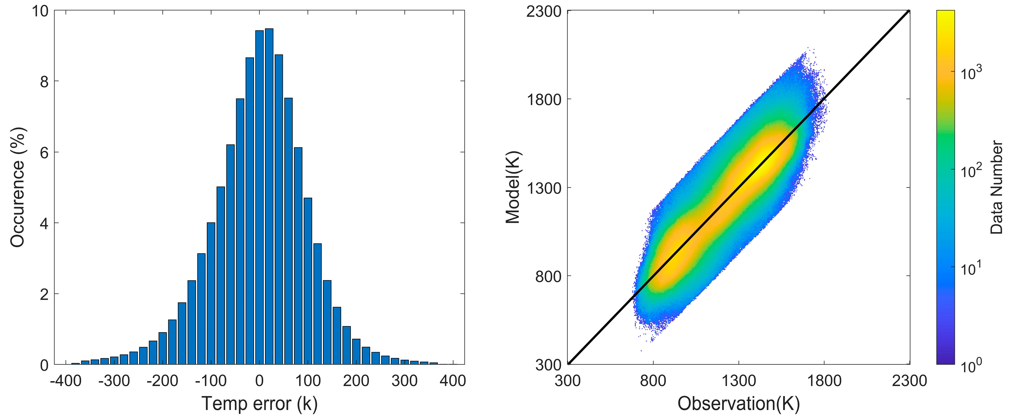
Figure 1 illustrates the distribution of errors and the comparison of the model values with the observed values. The median error of the model was 58.6 K. The slope of the fitting line between the observed and the model results was 1.0041. These results show that the empirical model fits the observed dataset very well. Subsequent model calculations were carried out to determine the results at an altitude of 600 km under a moderate solar activity condition (F107 = 140).
In this study, the Angle between the horizontal projection of the Magnetic Field line and the Sunrise line (AMFS) was defined as the difference in geographical longitude between the origins of the magnetic field lines in the northern and southern hemispheres, minus the difference in geographical longitude between the sunrise lines at the corresponding geomagnetic latitudes, i.e.,
wherein
represents the difference in geographical longitude between the origins of the magnetic field lines,
and
denote the corresponding geographical longitudes in the northern and southern hemispheres,
represents the difference in geographical longitude between the sunrise lines at the corresponding geomagnetic latitudes, and
and
denote the corresponding geographical longitudes in the northern and southern hemispheres.
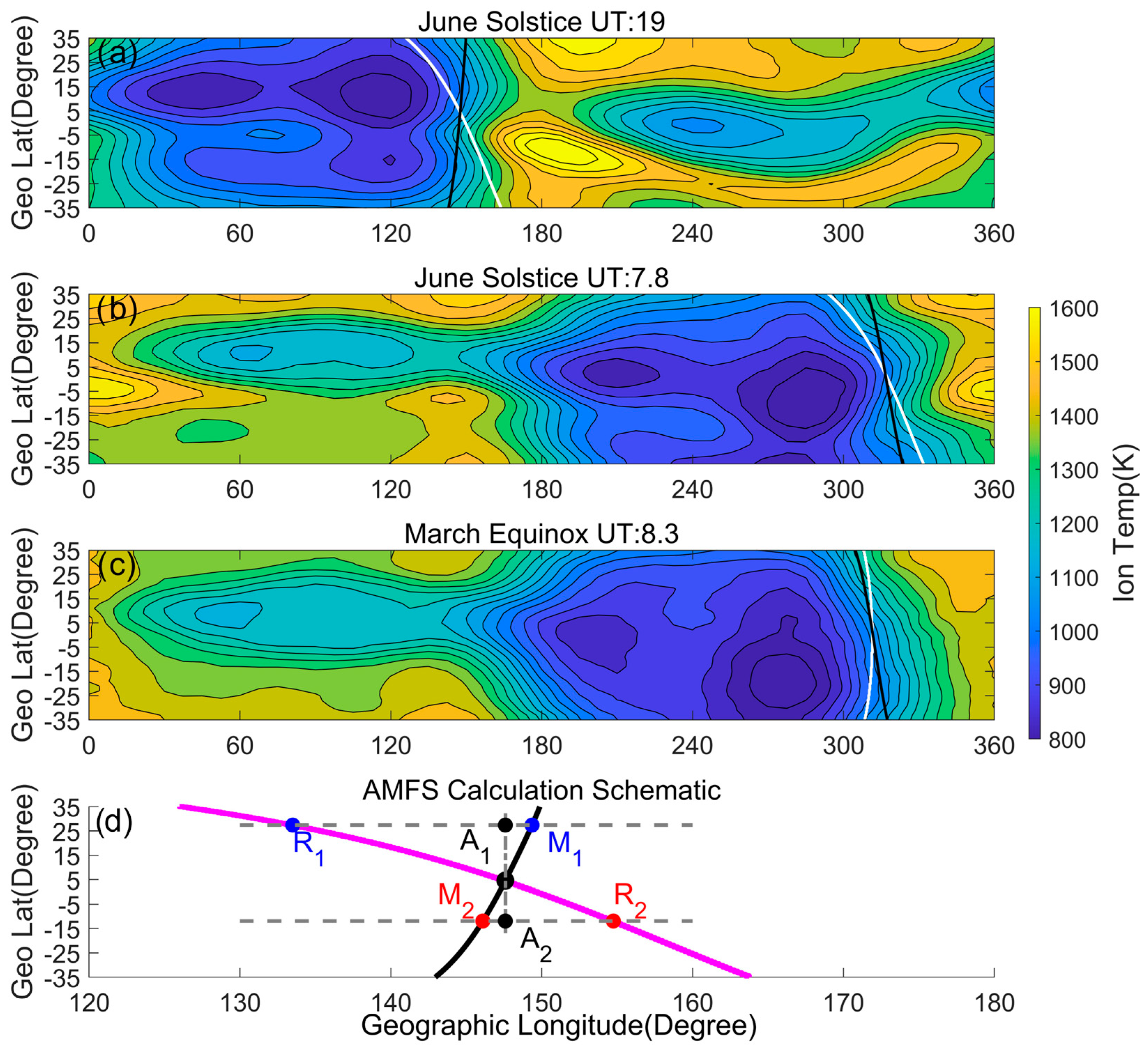
Figure 2d illustrates the definition and the calculation of the AMFS. Using the International Geomagnetic Field model [
27], we first traced the magnetic field lines originating from different geomagnetic latitudes (ranging from 3° to 30°) in various longitudinal sectors at an altitude of 600 km. After that, we traced the magnetic field line to an altitude of 200 km, so that the horizontal projection of the magnetic field line and the sunrise line were on the same plane, obtaining the values of L
M1 and L
M2. Then, we computed the position of the sunrise lines at an altitude of 200 km at the corresponding geomagnetic latitudes, obtaining the values of L
R1 and L
R2. Then, we could finally calculate the value of the AMFS. At the same time, we also calculated the lengths of the magnetic field lines (LMFs) from different magnetic latitudes. Since the photoelectrons are mainly transported along the magnetic field line at altitudes above 300 km, the calculation of the length of the magnetic field lines is based on the segment from 300 km in the anterior sunrise hemisphere to 600 km in the posterior sunrise hemisphere.
The intensity of predawn heating is defined as the difference between the ion temperature of the posterior sunrise hemisphere at sunrise and the anterior sunrise hemisphere at sunrise.
Figure 2d illustrates the positions of the two calculated points in the northern and southern conjugated hemispheres. The intensity of predawn heating was calculated as
, where T
A2 represents the ion temperature at the A2 point at sunrise and T
A1 represents the ion temperature at the A1 point at sunrise.
Figure 2a–c illustrate some examples of predawn heating of ion temperatures during the June solstice and the March equinox. The relative positions of the magnetic field lines in the horizontal projection (black lines) and the sunrise lines (white lines) are also shown in the figure. As shown in
Figure 2a, the magnetic field line has a significant angle with the sunrise line, which means the AMFS is considerably high. Thus, we can see a significant increase in the ion temperature at sunrise in the southern hemisphere. However, if the angle is significantly reduced, as shown in
Figure 2b, the predawn heating effect is significantly reduced. The northern and southern hemispheres have the same sunrise time during the March and September equinoxes. Therefore, in this situation, it is not easy to produce the predawn heating effect. However, if the magnetic field line has a large enough deflection angle in some longitudinal sectors, such as in the 315–330° sector, the predawn heating effect can still be produced, as shown in
Figure 2c.
3. Data Analysis and Result
The above results suggest that the AMFS is indeed an essential factor affecting predawn heating. Therefore, based on the empirical ion temperature model constructed above, we conducted a quantitative study to investigate the effect of the AMFS on predawn heating. Previous studies on the intensity of the predawn heating effect have primarily focused on the length of the magnetic field lines, suggesting that the heating rate decreases with the increase in the LMF [
20]. Utilizing the ion temperature model constructed above, we have also quantitatively investigated the impact of the LMF on the predawn heating effect. By employing the ion temperature model, we simulated the ion temperature in the global middle and the low-latitude topside ionosphere at an altitude of 600 km under moderate solar activity conditions on different days, with day numbers ranging from 5 to 365, at intervals of 5 days.
Firstly, we examined the impact of the AMFS.
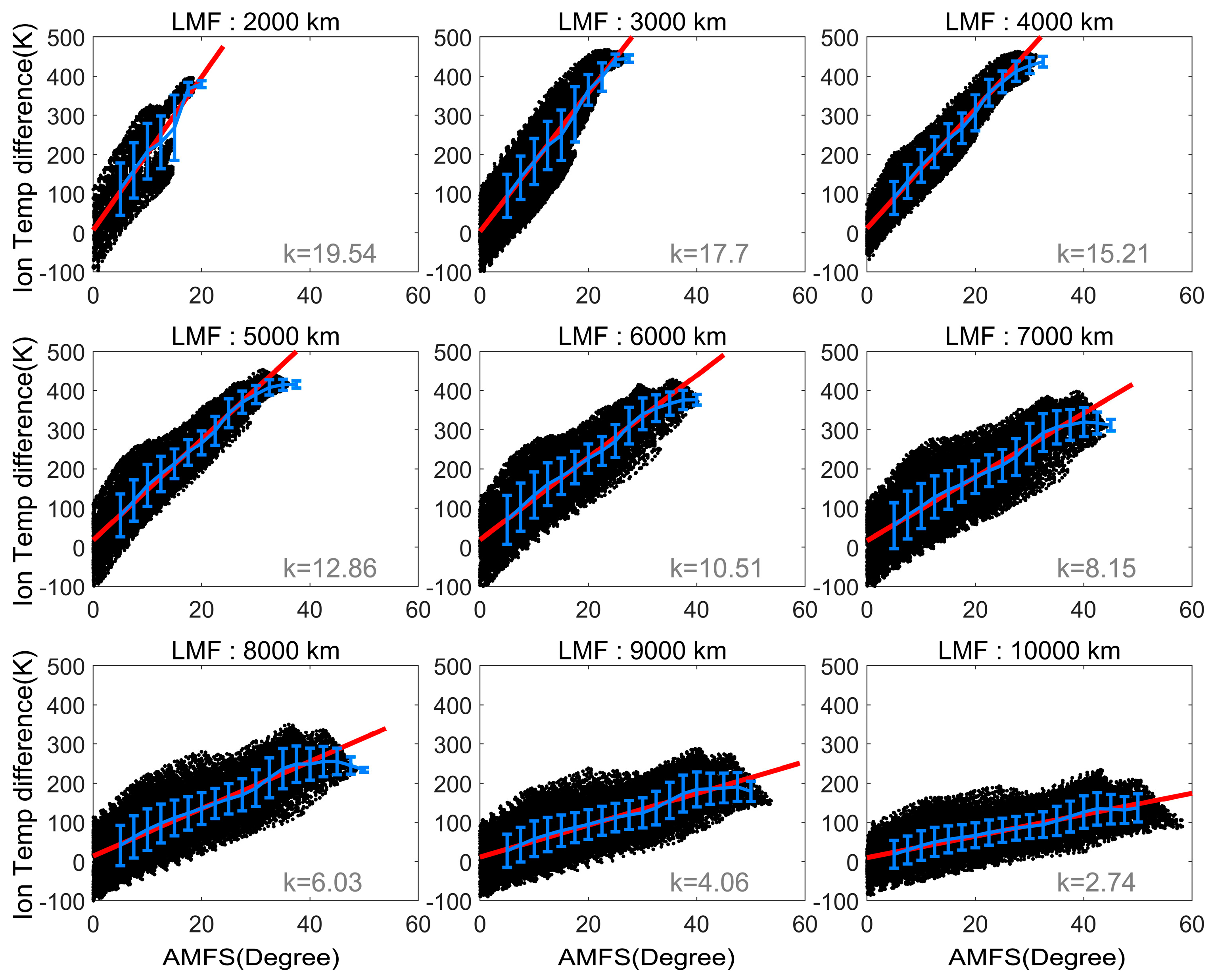
Figure 3 illustrates the variation in ion temperature increase with the AMFS at approximately the same LMF value. For each panel, the data include results within ±10% of the center LMF value. The red line in the figure represents the fitting line for the scatter points, with k being the slope of the fitting line. We separately calculated their relationship with the LMF values ranging from 2000 km to 10,000 km. The statistical results indicate that the AMFS has a significant impact on the predawn enhancement in ion temperature. For the same LMF, the larger AMFS results in a greater ion temperature increase, and thus a stronger effect on predawn heating. The k value reflects the efficiency of AMFS in influencing the predawn heating effect. As the LMF increases, the k value gradually decreases. That is, for regions with longer magnetic field lines at higher latitudes, a larger AMFS would be required to achieve the same predawn ion temperature increase. This implies that the influence of the AMFS on the predawn ion temperature increase is reduced as the LMF increases.
We further investigated the impact of the LMF on predawn heating.
Figure 4 illustrates the variation of predawn heating with varying LMFs, with the AMFS values ranging from 5 degrees to 45 degrees with a span of plus or minus 2.5 degrees. The statistical results indicate that under conditions where the AMFS is approximately the same, the longer the LMF is, the weaker the predawn heating effect is. The k absolute value reflects the efficiency of the LMF in blocking predawn heating. As the AMFS increases, the k absolute value gradually increases. That is, for longitudinal sectors and seasons with smaller AMFS, a shorter LMF would be required to achieve the same predawn ion temperature increase. This implies that the effect of the LMF on the predawn ion temperature rise increases with increases in the AMFS. By comparing
Figure 3 and
Figure 4, we can observe that the correlations between the predawn heating effect and LMF and between the predawn heating effect and AMFS are strong, which suggests that the predawn heating effect is jointly controlled by the AMFS and the LMF.
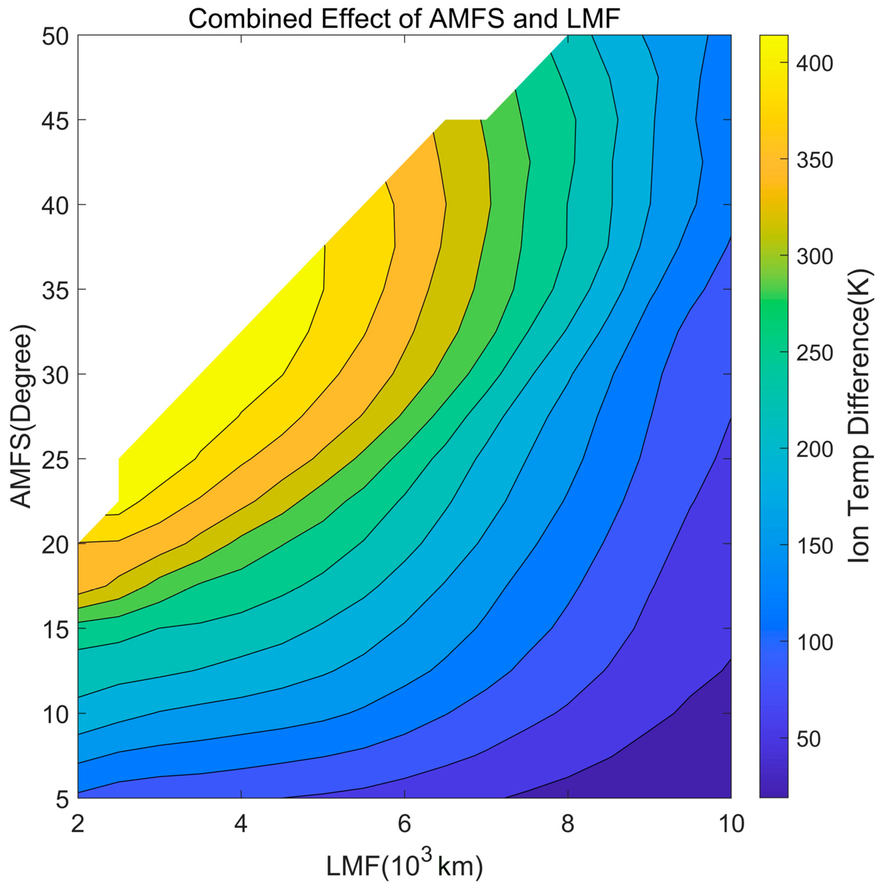
As mentioned above, the predawn heating effect is influenced by both the LMF and the AMFS. An increase in an LMF value decreases the predawn heating effect. Conversely, an increase in the AMFS value increases the predawn heating effect. In addition, with the increase in geomagnetic latitude, the LMF will gradually increase for the same longitude sector; the AMFS will also become larger. To comprehensively consider the combined effects of the LMF and the AMFS on the ion predawn heating effect, we further calculated the average predawn heating effect under different conditions, with the LMF values ranging from 2000 to 10,000 km and the AMFS ranging from 5 to 50°.
Figure 5 presents a contour map showing the predawn heating as a function of the LMF and the AMFS. This result clearly shows how the AMFS and the LMF work together to influence predawn heating. We found that the predawn heating effect is most significant when the AMFS value is about 30 degrees, and the LMF value is around 4000 km. In this scenario, the ion temperature increased by more than 400 K. As the length of the magnetic field lines increases, the strongest predawn heating occurs at larger AMFS values, which can also be seen in the trends in the error bar charts in
Figure 3.
4. Discussion
The AMFS reflects the difference in the sunrise time at the northern and southern ends of the same magnetic field line. When the AMFS approaches zero, the northern and the southern hemispheres of the same magnetic field line experience sunrise simultaneously, regardless of whether the magnetic field line deviates from geographical meridians. Conversely, when the AMFS value is higher, there will be a difference in the sunrise time between the northern and the southern hemispheres of the same magnetic field line. Moreover, the larger the AMFS, the greater the difference in sunrise time between the conjugated northern and southern hemispheres along the magnetic field line. This will cause the photoelectrons from the hemisphere that experiences the sunrise first to travel along the magnetic field line to the conjugated hemisphere earlier, thereby causing earlier and longer-lasting heating and generating a stronger predawn heating effect. Considering the important impact of the AMFS, predawn heating will not only occur near the solstices but can also occur during other seasons, even at the equinoxes with large AMFS values.
The influence of the LMF on predawn heating is primarily due to heat loss, which results from collisions between the photoelectrons and the surrounding plasma during their trans-hemispheric transportation. The longer the LMF is, the greater the integrated electron content along the field line will be, leading to greater loss of photoelectrons during their trans-hemispheric transportation. Consequently, fewer electrons will reach the conjugated hemisphere, resulting in a weaker heating effect.
Although the AMFS can enhance the heating effect, there is a ceiling to this enhancement, which we have called the saturation effect. When the LMF is longer than 8000 km and the AMFS is larger than about 35 degrees, even if the AMFS continues to increase, the heating effect will no longer increase. Similarly, as with the case of a small AMFS, the impediment effect of a longer LMF on predawn heating is also subject to the saturation effect.
5. Summary and Conclusions
In this study, we utilized an extensive dataset of topside ionosphere ion temperatures from the Rocsat-1 satellite to develop a global ion temperature model for middle and low latitudes. Employing a gridded approach, our model demonstrated a median error of 58.6 K when compared to the observational data. Subsequently, we employed an established empirical ion temperature model to simulate the global distribution of topside ionosphere ion temperatures across the different seasons.
Our analysis highlighted the predawn heating effect, focusing on two critical factors: the angle between the horizontal projection of the magnetic field line and the sunrise line (AMFS) and the length of the magnetic field line (LMF). We introduced the AMFS as a novel key factor influencing predawn heating, complementing the previously recognized important factor, the LMF. Through quantitative analysis, we established that the predawn ion heating is significantly influenced by both the AMFS and the LMF. Our findings indicate that an increase in the AMFS enhances predawn heating, while the heating effect weakens with an increasing LMF. Notably, the impact of the LMF on predawn ion temperature is more pronounced at higher AMFS values.
Through comprehensive statistical analyses of ion heating across a range of LMF values spanning 2000 to 10,000 km and the AMFS values from 5° to 50°, we identified an optimal condition for maximum predawn heating. This occurs when the LMF is approximately 4000 km long, and the AMFS is around 30 degrees, where the combined effect of the AMFS and the LMF is most pronounced, reaching more than 400 K. Additionally, we observed that both the AMFS and the LMF exhibit saturation effect.


