Technical Note

Intelligent Recognition of Coastal Outfall Drainage Based on Sentinel-2/MSI Imagery

1
Southern Marine Science and Engineering Guangdong Laboratory (Guangzhou), Guangzhou 511458, China
2
School of Oceanography, Shanghai Jiao Tong University, Shanghai 201100, China
3
State Key Laboratory of Satellite Ocean Environment Dynamics, Second Institute of Oceanography, Ministry of Natural Resources, Hangzhou 310012, China
4
Donghai Laboratory, Zhoushan 316021, China
*
Author to whom correspondence should be addressed.
Remote Sens. 2024, 16(2), 423; https://doi.org/10.3390/rs16020423
Submission received: 18 December 2023 / Revised: 15 January 2024 / Accepted: 16 January 2024 / Published: 22 January 2024

Abstract

:
In this study, we developed an innovative and self-supervised pretraining approach using Sentinel-2/MSI satellite imagery specifically designed for the intelligent identification of drainage at sea discharge outlets. By integrating the geographical information from remote sensing images into our proposed methodology, we surpassed the classification accuracy of conventional models, such as MoCo (momentum contrast) and BYOL (bootstrap your own latent). Using Sentinel-2/MSI remote sensing imagery, we developed our model through an unsupervised dataset comprising 25,600 images. The model was further refined using a supervised dataset composed of 1100 images. After supervised fine-tuning, the resulting framework yielded an adept model that was capable of classifying outfall drainage with an accuracy rate of 90.54%, facilitating extensive outfall monitoring. A series of ablation experiments affirmed the effectiveness of our enhancement of the training framework, showing a 10.81% improvement in accuracy compared to traditional models. Furthermore, the authenticity of the learned features was further validated using visualization techniques. This study contributes an efficient approach to large-scale monitoring of coastal outfalls, with implications for augmenting environmental protection measures and reducing manual inspection efforts.

1. Introduction

Amid swift societal progress and urbanization, issues surrounding aquatic environmental pollution have increasingly attracted attention [1]. Outfalls are recognized as principal conduits for pollutants to infiltrate recipient water bodies, such as oceans or rivers [2], making the monitoring of outfalls an essential and effective tool for water resource pollution surveillance. Oceans concurrently act as the ultimate repository for terrestrial pollutants [3]. In parallel, the discharge of treated domestic and industrial wastewater into oceans emerges as an economically sustainable approach for utilizing marine environments and mitigating the pressures on local environments. This strategy also serves as one of the predominant methods for sewage discharge in coastal regions, which underscores the importance of thorough coastal outfall monitoring.
The adoption of remote sensing technology in coastal outfall monitoring offers the dual advantages of continual surveillance and accessibility to remote or challenging locations, thus delivering temporal and spatial benefits. The successful application of this technology to tasks including river outfall location detection, abnormal water body classification from coastal outfalls, and impact area estimation of coastal outfall pollution signifies the potential for versatile implementation of remote sensing technology in coastal outfall monitoring. The rapid location of outfall positions over extensive areas can be achieved using high-resolution unmanned aerial vehicle (UAV) remote sensing combined with object detection methodologies [4]. To enhance this approach, the integration of geographical location activation and digital terrain models in multisource data fusion substantially boosts detection precision and recall rates. Regarding the classification of coastal outfalls, Anna et al. utilized a random forest algorithm based on SAR imagery to perform binary classifications of outfall plumes in the Gaza region, successfully distinguishing these plumes from other features [5]. Other researchers have developed random forest-based water body classification algorithms using satellite remote sensing imagery from the MultiSpectral Instrument (MSI) onboard the Sentinel-2 satellites to segregate water bodies into 14 distinct categories, thus facilitating the identification of detrimental discharge waters [6]. V. G. Bondur et al., employed band combinations to generate sea surface color indices [7], thereby effectively assessing the extent of impact engendered by coastal outfall discharges. Nevertheless, these methodologies present limitations in determining whether the outfalls are actively discharging wastewater into the ocean. For instance, classification approaches based on water bodies require prior knowledge of whether the coastal outfall is discharging water to further distinguish whether the discharge is sewage. Therefore, the primary objective of this research study is to develop a novel remote sensing methodology that enables precise monitoring of the drainage status of coastal outfalls over extensive areas. Equipped with pre-collected, valid outfall location data, this method is expected to detect whether each outfall site is actively discharging wastewater into the ocean, thus providing rapid alerts for the regulatory authorities.
Deep learning algorithms, specifically convolutional neural networks (CNNs), have gained recognition in the area of complex spatial pattern recognition, thus becoming invaluable in remote sensing applications, including scene classification [8]. Scene classification assigns remote sensing image blocks into land cover or land use types, benefiting from deep learning’s superior feature extraction ability to understand images semantically [9,10]. Despite their potential, deep learning methods rely on substantial, high-quality annotated datasets [11], a requirement that is often challenging to fulfill. Thus, self-supervised learning, which exploits proxy tasks on extensive unlabeled data for the learning of deep features, emerges as a solution, with outcomes that can, in some instances, surpass those of supervised learning [12]. The application of self-supervised learning is widespread in remote sensing image scene classification and methods, such as MoCo [13], Simsiam [14], and BYOL [15], have already proven successful [16]. Strategies incorporating geographical location information have displayed notably good performance, suggesting their potential utility in our proposed method [17,18].
Our main goal is to overcome the limitations of current methods by employing a self-supervised learning model, leveraging Sentinel-2/MSI imagery, to enhance the accuracy of outfall drainage classification, a task that is traditionally hampered by a scarcity of labeled data. In the present study, we assembled both a large-scale unsupervised dataset and a small-scale supervised dataset utilizing Sentinel-2/MSI images. We applied a self-supervised pretraining strategy that incorporates geographical information to enhance the performance of convolutional neural networks (CNNs) in outfall classification tasks. By doing so, we intend to develop a classification model that surpasses supervised methods in performance, thereby addressing the prevalent issue of a limited quantity of labeled images of outfalls.
The remainder of this paper is organized as follows: Section 2 describes the data and methods used in our study, including the details of the data preparation and the establishment of the intelligent recognition model. Section 3 presents the results of our analysis, focusing on the model performance and its evaluation. Finally, Section 4 concludes the paper with a summary of our findings and a discussion of their implications and potential future work.

2. Data and Methods

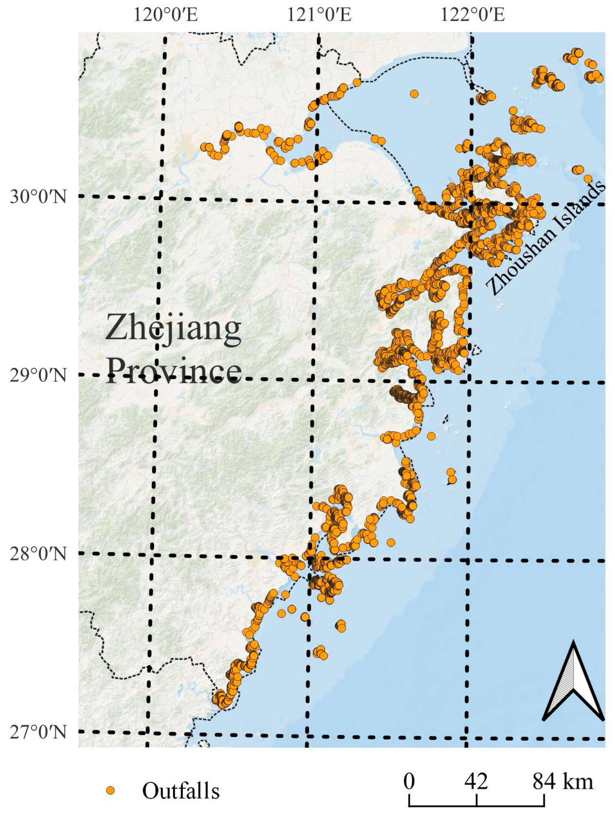
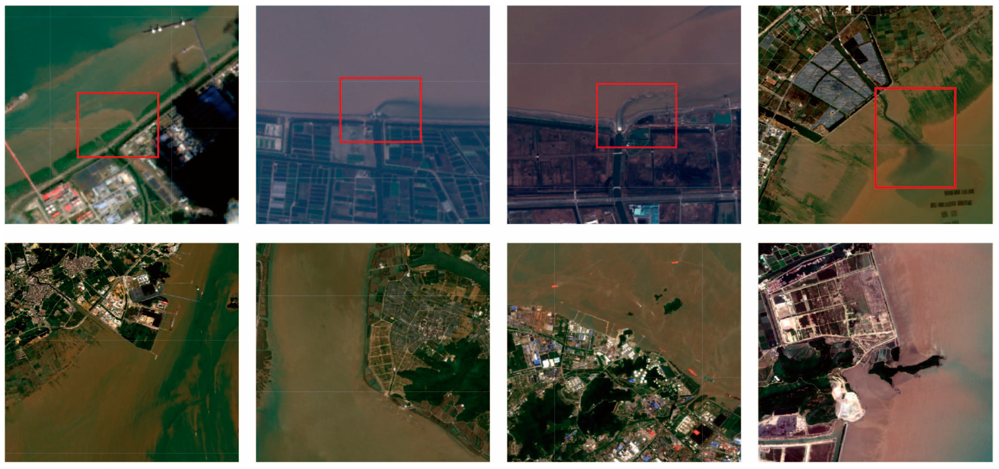
2.1. Data Preparation

This study utilizes true-color images acquired from the Sentinel-2 multispectral imager to construct both supervised and unsupervised datasets. The Sentinel-2A and Sentinel-2B satellites, launched by the European Space Agency on 23 June 2015 and 7 March 2017, respectively, maintain a revisit cycle of up to five days at the equator with the two satellites combined. Both Sentinel-2A and 2B satellite data are used. The MultiSpectral Instrument (MSI) embedded in these satellites offers imaging capabilities across 13 bands, ranging from visible to near-infrared, with the highest resolution of visible light bands reaching 10 m. The superior resolution and complimentary accessibility of Sentinel-2 data have not only led to their widespread utilization in land cover classification but also demonstrated promising applications in climate change, fire monitoring [19], and river pollution monitoring [20], as well as in algal bloom detection [21] and marine water quality assessment [22].
In this research study, the Sentinel-2 data utilized in our study were acquired from the Copernicus Open Access Hub. We used the true-color bands (with wavelengths of 490 nm, 560 nm, and 665 nm) from Level-2A products, which have a spatial resolution of 10 m. Sentinel-2 Level-1C (L1C) data are processed for radiometric calibration and basic geometric corrections, ensuring accurate reflection of captured electromagnetic energy and spatial consistency. Level-2A (L2A) data further enhance this by adding atmospheric correction to adjust for atmospheric effects on reflectance and incorporating cloud detection and masking. Through meticulous investigation and compilation of coastal outfall locations in Zhejiang Province, China, we acquired geographical information pertaining to these outfalls (Figure 1). The supervised dataset was manually annotated through visual interpretation using Google Earth Engine. This process involved categorizing images collected from 2017 to 2022 into two categories: outfall and non-outfall (Figure 2). This dataset comprises a total of 1100 images. The unsupervised dataset was generated by procuring corresponding images predicated on the location information and amalgamating multiple temporal data for the same locations. This step served as the foundation for selecting positive sample pairs in the subsequent steps. The unsupervised dataset comprises 25,600 images. All images were projected onto the UTM Zone 51 N coordinate system, and each image window measures 512 pixels in width and height, corresponding to an actual ground area of 5120 m by 5120 m. In the unsupervised dataset, a distance matrix was generated based on the distances between the different locations and saved as an integral component of the dataset. This matrix offers acceleration for the subsequent distance retrieval process.

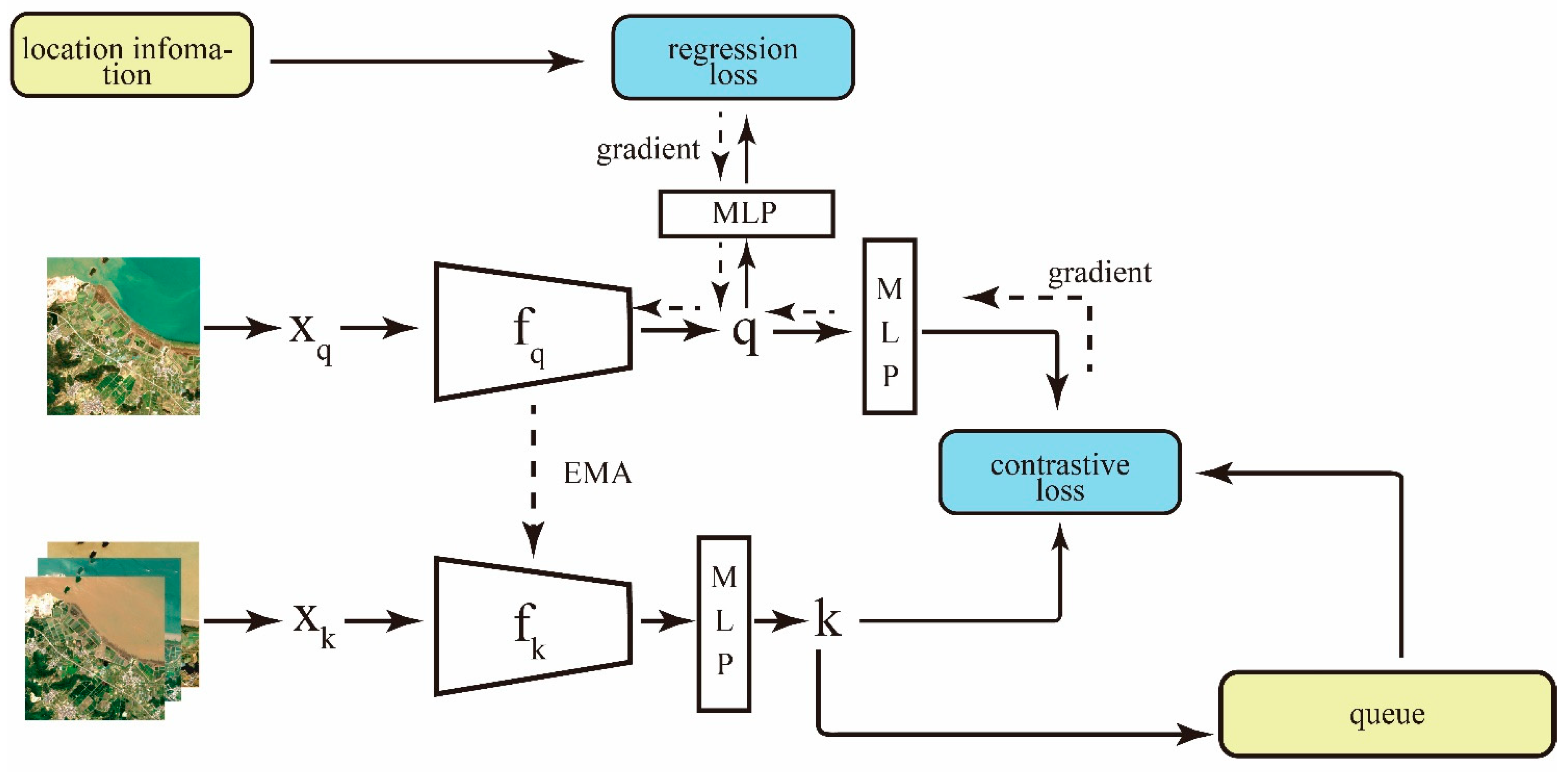
2.2. Establishment of the Intelligent Recognition Model

In the present study, we devised a self-supervised pretraining strategy anchored in contrastive learning while integrating a geographical coordinate prediction head to assist the encoder in the next stage of learning. To identify positive and negative sample pairs, we supplemented conventional image augmentation techniques with a mechanism that accommodates multiple temporal images and overlapping images. Moreover, we employed a dropout method analogous to SimCSE [23] for the generation of positive sample pairs. During the encoder’s parameter updating process, we aimed to conserve more sample encoding features without surpassing the GPU memory limit. To achieve this, we stored prior encoding features in a queue located in memory. This queue has the capacity to retain encoding features for a relatively extended period, and when used in conjunction with the momentum updates of parameters, it ensures the stability of the encoder’s parameters. This concept originated from and found success in the MoCo method [13].
Our training process is illustrated in Figure 3. The process begins with the input of satellite imagery into the ResNet-50 encoder, which is responsible for converting raw data into a sophisticated set of feature representations. These features are then encoded into two distinct formats: ‘q’ (query) and ‘k’ (key), each playing a vital role in the model’s analysis. The encoded features are processed by a projection head, typically comprising a multilayer perceptron, to prepare them for the classification task. A crucial aspect of our model is the simultaneous application of contrastive loss and geolocation loss (Lg). The contrastive loss assesses the similarity between the ‘q’ and ‘k’ encodings, which are crucial for learning discriminative features from the unlabeled data. Concurrently, the geolocation loss integrates geographical context, enabling the model to capture spatial relationships and nuances within the imagery more effectively. This dual-loss approach enhances the model’s ability to recognize and classify drainage patterns accurately. The final output of the model is a classification of the imagery, categorizing it based on the identified drainage patterns and leveraging the enhanced feature representations developed through this comprehensive, dual-loss-informed learning process.
(1)
Training Framework
We define the unsupervised dataset as X = { x i | i = 1 , , N } , where x q and x k form positive sample pairs. Specifically, x q is from the original dataset, while x k is an image selected from X and subjected to image augmentation, which will be explained in detail in the next section. At the initial stage, f q and f k are two identical encoders. The encoder is defined as a function: f θ ( x ) : R H × W × C R d , where H , W , and C represent the width, height, and number of channels of the image, respectively, and d is the dimension of the feature vector. The encoder f q updates its parameters through gradient backpropagation, while the gradient does not propagate to the encoder f k . The encoder f k slowly updates its parameters using an exponential moving average (EMA) based on the encoder f_q, with the update process as follows:
θ q t = β θ q t 1 + ( 1 β ) θ k t 1
where θ e t ( e { k , q } ) represents the parameters of the encoder at time t , and β is a parameter less than 1 that controls the updating speed, which we set to 0.999. After passing through the encoder, we obtain the encodings q and k , which are then fed into a multilayer perceptron (MLP) with two linear layers ( e θ ( x ) : R d R d ). To ensure that the encoder learns meaningful information in the self-supervised task, the contrastive learning proxy task is designed to pull the encoding features of positive sample pairs closer while pushing the encoding features of positive and negative sample pairs further apart. Therefore, we use the InfoNCE function [24] as the contrastive loss, which can be represented as L c :
L c = l o g e x p ( e q ( f q ( x q ) ) e k ( f k ( x k ) ) / λ ) e x p ( e q ( f q ( x q ) ) e k ( f k ( x k ) ) / λ ) + j = 1 M e x p ( e q ( f q ( x q ) ) k j / λ )
The negative samples { k j } j = 1 M are obtained from the queue maintained in memory, where M is a fixed length and the queue follows a first-in-first-out principle, which allows us to maintain a sufficiently large set of negative samples without loading a large amount of data into the GPU’s memory each time. λ is a temperature parameter that controls the width distribution of the function. The encoder q is then passed through another layer of MLP and projected into a two-dimensional vector, i.e., e g ( q ) = [ l x ^ , l y ^ ] . This vector is used to calculate the location loss, which is referred to as ‘regression loss’ in Figure 3, in conjunction with the geographical information from the following labels:
L g = 1 2 [ ( l x l x ^ ) 2 + ( l y l y ^ ) 2 ]
where l x and l y represent the coordinates of the center point of the original image after projection in the projected coordinate system. Finally, we linearly combine the two loss components, where α is a parameter used to indicate the relative importance of the two loss components. The overall objective of this self-supervised learning is represented as follows:
a r g   m i n L θ q , θ k , θ g = α L c + ( 1 α ) L g
(2)
Positive Sample Pair Generation
Standard methodologies for the generation of positive sample pairs typically involve capturing varying perspectives of an identical image, achieved by deploying image augmentation methods, such as rotation, cropping, and color transformations, resulting in images derived from the original [11]. While this approach has seen success in the realm of computer vision, it does not fully exploit the surplus information that is inherent in remote sensing images. Hence, we propose a filtering mechanism underpinned by geographical location and temporal data. During the dataset construction process, we maintained corresponding location data for each point and formulated a distance matrix grounded in these points. This approach facilitates the retrieval of the distance between any two given points. By setting a distance threshold denoted as d , we filter out points that exhibit a certain degree of overlap with a specific image. Furthermore, considering the fact that images of an identical location may display temporal variations, we select images from different timeframes as candidate images from the filtered points. From this candidate pool, we randomly select one image to form a positive sample pair with the original image.
The carefully selected positive sample pairs are subjected to an array of augmentation techniques, encompassing random rotation, cropping, grayscale transformation, Gaussian blur, color modifications, and occlusion. Furthermore, we adopt the random dropout method utilized in SimCSE [23]. This involves applying distinct dropout masks to encoders sharing identical parameters, thereby engendering marginally diverse encodings for the same image. Originally, the dropout strategy was conceived to mitigate overfitting through the deactivation of certain neurons during the training process. This results in slightly varied output features under constrained data conditions, thereby reducing the propensity for overfitting.
Through the strategic deployment of these filtering and augmentation methods, we ascertain that the images, while maintaining similarities in their semantic features, display divergences in both visual appearance and encoding features. Our objective is for the encoder to learn the intrinsic connections between these images in the absence of labeled data via contrastive self-supervised learning. Consequently, this methodology provides a high-quality pre-trained model for subsequent supervised training endeavors.
(3)
Feature Assessment and Visualization
In an effort to visually authenticate the effectiveness of our model and evaluate the learned features during the training phase, we engaged Grad-CAM++ [25] to facilitate the visualization of the convolutional neural network (CNN) model. Grad-CAM++ serves as an enhancement to Grad-CAM [26], offering superior visualization results, particularly for multiple and smaller objects. It computes the weights of each channel in the feature map and subsequently conducts guided backpropagation to acquire the visualization results on the original image. This is achieved by computing derivatives of the specific class output and preserving positive derivatives. For any spatial position ( i , j ) of the saliency map pixel L i j c , which corresponds to class c , the calculation is executed as follows:
L i j c = R e L U ( k w k c A i j k )
w k c = i j α i j k c R e L U ( Y c A i j k )
α i j k c = 2 Y c ( A i j k ) 2 2 2 Y c ( A x j k ) 2 + a b A a b k { 3 Y c ( A i j k ) 3 }
where A i j k denotes the value of the k-th layer in the feature map, Y c signifies the output value corresponding to class c , and the rectified linear unit (ReLU) function serves as an activation function frequently utilized within the framework of neural networks:
R e L U ( x ) = m a x ( 0 , x )
We further adopted the technique of guided backpropagation [27]. Guided backpropagation is a deep learning visualization method that operates by modifying the standard backpropagation process. In conventional backpropagation, error gradients propagate from the output layer back to the input layer, computing contributions to the output. In guided backpropagation, this method is modified to propagate gradients only when both the input and gradient are positive. Thus, the modified gradient propagation rule becomes as follows:
f x = { 1 ,       i f   x > 0   a n d   f x > 0   0 ,       o t h e r w i s e
This means that the gradient is allowed to backpropagate through the layer only if both the input x and the gradient of the layer with respect to the loss function L , L f , are positive. This selective backpropagation helps filter out features that do not positively contribute to the model output, thereby emphasizing those features that are most influential in the model’s decision-making in visualizations.
(4)
Evaluation of Model Performances
In our analysis, we employ two primary metrics to evaluate the performance of our model: accuracy and the F1-score. Accuracy is defined as the proportion of true results (both true positives and true negatives) among the total number of cases examined. Mathematically, it is expressed as follows:
Accuracy   =   True   Positives   ( TP )   +   True   Negatives   ( TN )     TP   +   False   Positives   ( FP )   +   False   Negatives   ( FN )   +   TN  
The F1-score is a measure that combines precision and recall, both of which are critical in scenarios where imbalanced class distribution is present. Precision is the ratio of true positives to all positive predictions, while recall is the ratio of true positives to all actual positives. The F1-score is the harmonic mean of precision and recall, providing a balance between them. It is calculated as follows:
F 1 - score   = 2 ×   Precision   ×   Recall     Precision   +   Recall   ,
where
Precision   = TP TP + FP ,   Recall   = TP TP + FN
We utilize these metrics due to their ability to offer a comprehensive view of the model’s performance. Accuracy provides an overall effectiveness measure, while the F1-score offers insight into the balance between precision and recall.

3. Results and Discussion

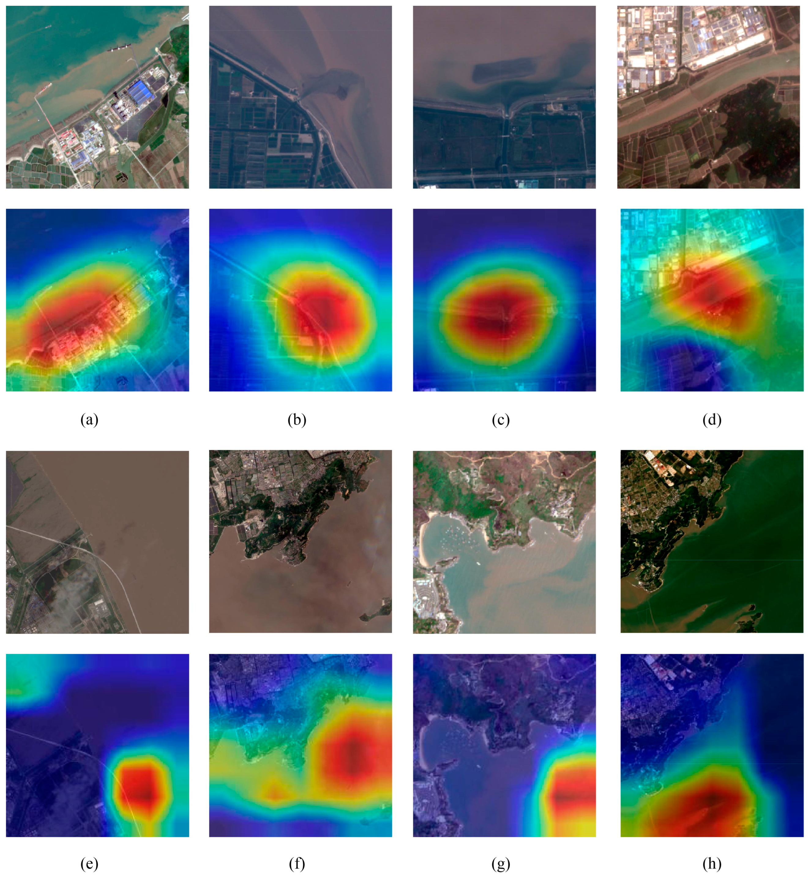
3.1. Visual Results from the Encoding Model

In our study, we also employed ResNet50 [28] as the encoding model. Following the pretraining and supervised fine-tuning processes, we proceeded with sample inference and visualization utilizing the methodology delineated below (Figure 4). The regions depicted in red correspond to areas bearing high weight, which are the key regions of interest from the model’s perspective. The results of guided backpropagation, to a certain extent, reflect the detailed image areas influencing the model’s decision-making process. A clear alignment is observed between these regions and the actual locations of the outfalls, thereby suggesting that the model has effectively learned pertinent features for classification throughout the training phase.

3.2. Pretraining Enhancement and Baseline Model Evaluation

To appraise the enhancements resulting from our pretraining approach, we employed a variety of baseline models for pretraining that were subsequently refined utilizing supervised classification models. A partition of 20% from the supervised dataset was designated as the testing set to evaluate classification accuracy, and the corresponding results are displayed in Table 1. To ensure that the experimental conditions remained consistent, ResNet-50 was adopted as the encoder (i.e., f q and f k ) across all self-supervised methodologies. Detailed descriptions of the various comparison baseline models are as follows:
(1)
Supervised-only: This method involves training the encoder exclusively on supervised data, maintaining complete isolation from the unlabeled dataset.
(2)
Self-sup-only: This self-supervised training method abstains from incorporating geographical information, thereby excluding the parameter update via L g , and geographical location information is not utilized in selecting positive sample pairs. The generation of positive sample pairs adheres to the same strategy as MoCo-V2 [29].
(3)
Selfsup + Geoloss: This method builds upon the previous approach, employing L g for gradient calculation and subsequent parameter updates.
(4)
Selfsup + Geoloss + GeoSelect: This method extends method 3, incorporating the sample pair selection mechanism, as discussed in Section 3.2.
Table 1. Test results with subsequent supervised datasets for models pre-trained with different baseline methods. Values in bold indicate the best performance for each metric.
MethodsEncoderAccuracy (%)F1-Score (%)
Supervised-onlyResnet5079.7375.68
Selfsup-onlyResnet5084.2381.67
Selfsup + GeolossResnet5088.2986.17
Selfsup + Geoloss + GeoSelectResnet5090.5488.52
The experimental results clearly demonstrate that unsupervised pretraining significantly enhances model performance in remote sensing image scene classification tasks compared to supervised training alone. Specifically, a Resnet50 model trained with supervision only achieved an accuracy of 79.73% and an F1 score of 75.68% on the test set. Introducing unsupervised pretraining improved the accuracy to 84.23% and the F1 score to 81.67%, confirming the potential of unsupervised learning in extracting effective feature representations, even without explicit labels. Incorporating geographical loss (Lg) in unsupervised learning further increased the accuracy and F1 score to 88.29% and 86.17%, respectively, indicating the benefits of geographical information in representing remote sensing data by providing additional spatial context. The most significant improvement occurred when introducing a geographically based positive sample selection mechanism into unsupervised learning, resulting in the highest accuracy of 90.54% and F1 score of 88.52% among all methods. This highlights the significant impact of geographically filtering positive samples, likely due to the visual and semantic similarities of geographically proximate images, offering the model more similar yet distinct positive sample pairs for learning highly discriminative features.
Throughout the training process, methods 2–4, which require pretraining, retain consistent parameters. Each method undergoes 200 epochs of training with a batch size of 128. The initial learning rate is designated at 0.001, and it is progressively attenuated to 0.00001 as the experiment advances. The length of the memory queue is uniformly established at 65,536, with the distance threshold d defined as 500. The experimental results demonstrate that the weight parameter α in Equation (4) exerts a negligible influence on training accuracy, although it does modify the rate of convergence. For the purpose of this study, we set α = 0.9 . When compared to other contrastive self-supervised frameworks (Table 2), our method, which is Method 3, demonstrates optimal performance and achieves the most commendable outcomes.

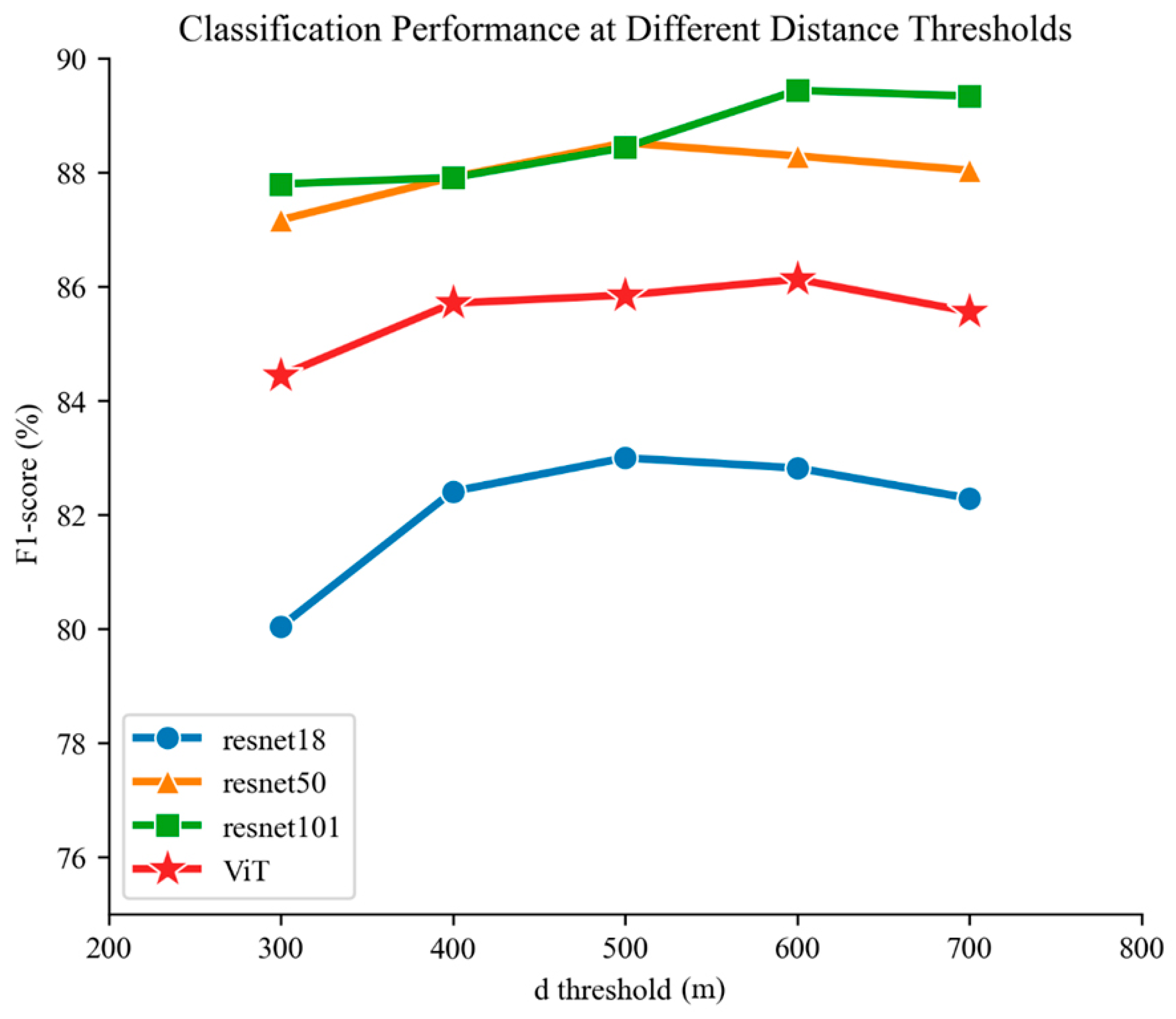
3.3. Impact of Distance Threshold on Encoder Performance

Additionally, the magnitude of the distance threshold d during the selection process can potentially affect the accuracy of the pre-trained model. Figure 5 illustrates the performance of distinct encoders at various threshold values. Among these encoders—ResNet-18, ResNet-50, ResNet101, and ViT [31]—there is an increase in parameter quantities.
Analyzing the F1 scores shown in the graph, we observe that the models based on the Resnet architecture exhibit an initial increase followed by a decrease in performance with rising distance thresholds, while ViT-based models show higher performance at smaller threshold ranges. There is a positive correlation between the number of encoder parameters and accuracy performance, but ViT does not follow this pattern. Thus, our algorithm may not be suitable for transformer-based models. This suggests an optimal balance in the quality of positive sample pairs at certain thresholds, reflecting spatial associations in remote sensing imagery while maintaining sufficient variability for model learning. Notably, the performance of Resnet50 and Resnet101 peaks at medium-distance thresholds, indicating that deeper networks may better capture and utilize complex spatial patterns in remote sensing data.

3.4. Analysis of Classification Outcomes

In Figure 6, we illustrate instances classified by our algorithm as actively draining when applied to real-world imagery that is not included in the training set. Notably, the regions of high relevance in the correctly classified positive samples align precisely with active drainage locations. Regarding the misclassified instances, the emphasized regions in Figure 6e,f correspond to areas with diminished brightness obscured by cloud shadows, while those in Figure 6g,h are situated in turbid water zones enriched with sediment. These two types of scenarios predominantly account for our misclassification outcomes.

4. Summary

Anthropogenic emissions have exerted substantial pressure on the coastal marine environment, requiring rigorous monitoring of coastal outfalls to safeguard the surrounding marine water systems. However, there is a noted deficiency in effective satellite remote sensing mechanisms for large-scale outfall drainage monitoring, compounded by a dearth of annotated data, which escalates the challenge of training effective classification models.
In the current research, we developed a self-supervised pretraining approach tailored for the visible light bands of Sentinel-2 remote sensing imagery, with the primary objective of classifying the drainage conditions of coastal outfalls. Following this, supervised fine-tuning enabled us to refine an efficient outfall classification model, thereby facilitating extensive monitoring of outfall statuses discharging into maritime regions. Notably, our training method effectively utilizes the geographic information embedded in the remote sensing imagery, delivering greater accuracy than methods that exclude such geographic data. Our method demonstrated an accuracy rate of 90.54%, significantly outperforming conventional models. A series of ablation experiments confirmed a 10.81% improvement in accuracy compared to traditional models, showcasing the effectiveness of our training framework. Additionally, through rigorous visualization techniques, we assessed the post-supervised training model, thereby validating the potency of the acquired features.
Our approach offers an innovative perspective on monitoring coastal outfalls. By meticulously tracking the drainage status, we can promptly identify specific drainage locales, subsequently redirecting our monitoring emphasis toward regions of particular interest. This approach not only economizes manual inspection efforts but also supports monitoring on an expansive scale. However, there are many factors that can degrade the performance of the proposed approach, such as cloud shadows and turbid waters. In the future, we will augment the classification precision by implementing preprocessing strategies in regions affected by cloud shadows and incorporating samples with distinct, analogous morphologies. Such advancements will further broaden our monitoring capacity, ensuring exhaustive surveillance of outfall statuses across an even more extensive area.
Currently, our approach focuses on identifying drainage presence without analyzing wastewater treatment status. Future improvements could include integrating additional data, like hyperspectral imagery or water quality measurements, to enhance classification capabilities.

Author Contributions

Conceptualization, X.H.; methodology, H.L. and X.H.; software, H.L. and F.G.; validation, F.G.; formal analysis, H.L. and X.H.; investigation, H.L. and D.W.; resources, X.H.; data curation, H.L. and T.L.; writing—original draft preparation, H.L.; writing—review and editing, X.H., Y.B. and D.W.; visualization, H.L. and T.L.; supervision, X.H.; project administration, X.H. and Y.B.; funding acquisition, X.H. All authors have read and agreed to the published version of the manuscript.

Funding

This research was funded by the “Pioneer” R&D Program of Zhejiang (2023C03011), the National Natural Science Foundation of China (Grants #U23A2037, #U22B2012, and #42176177), and the Zhejiang Provincial Natural Science Foundation of China (Grant #LDT23D06021D06).

Data Availability Statement

The dataset will be made available upon reasonable request.

Acknowledgments

We gratefully acknowledge the European Space Agency (ESA) Copernicus Open Access Hub for offering the Sentinel-2 data from https://scihub.copernicus.eu/dhus/#/home (accessed on 20 June 2022) used in this study. We are also grateful for the help with data collection and processing provided by the SOED/SIO/MNR satellite ground station, satellite data processing, sharing facility, and marine satellite data online analysis platform (SatCO2). Lastly, we express our profound thanks to the reviewers and the editor for their insightful and constructive feedback, which significantly enriched this manuscript.

Conflicts of Interest

The authors declare no conflicts of interest.

References

  1. Wang, Q.; Yang, Z. Industrial water pollution, water environment treatment, and health risks in China. Environ. Pollut. 2016, 218, 358–365. [Google Scholar] [CrossRef]
  2. Zhang, J.; Zou, T.; Lai, Y. Novel method for industrial sewage outfall detection: Water pollution monitoring based on web crawler and remote sensing interpretation techniques. J. Clean. Prod. 2021, 312, 127640. [Google Scholar] [CrossRef]
  3. Huang, Y.; Wu, C.; Yang, H.; Zhu, H.; Chen, M.; Yang, J. An Improved Deep Learning Approach for Retrieving Outfalls Into Rivers From UAS Imagery. IEEE Trans. Geosci. Remote Sens. 2021, 60, 1–14. [Google Scholar] [CrossRef]
  4. Xu, H.; Huang, Q.; Yang, Y.; Li, J.; Chen, X.; Han, W.; Wang, L. UAV-ODS: A Real-time Outfall Detection System Based on UAV Remote Sensing and Edge Computing. In Proceedings of the 2022 IEEE International Conference on Unmanned Systems (ICUS), Guangzhou, China, 28–30 October 2022; pp. 1–9. [Google Scholar]
  5. Ballasiotes, A.D. Mapping Untreated and Semi-Treated Wastewater Effluent off the Coast of Gaza with Sentinel-1 Time Series Data. Master’s Thesis, Oregon State University, Corvallis, OR, USA, 2020. [Google Scholar]
  6. Wang, Y.; He, X.; Bai, Y.; Tan, Y.; Zhu, B.; Wang, D.; Ou, M.; Gong, F.; Zhu, Q.; Huang, H. Automatic detection of suspected sewage discharge from coastal outfalls based on Sentinel-2 imagery. Sci. Total Environ. 2022, 853, 158374. [Google Scholar] [CrossRef]
  7. Bondur, V.; Zamshin, V.; Zamshina, A.S.; Vorobyev, V. Registering from space the features of deep wastewater outfalls into coastal water areas due to discharge collector breaks. Izv. Atmos. Ocean. Phys. 2020, 56, 979–988. [Google Scholar] [CrossRef]
  8. Yuan, Q.; Shen, H.; Li, T.; Li, Z.; Li, S.; Jiang, Y.; Xu, H.; Tan, W.; Yang, Q.; Wang, J. Deep learning in environmental remote sensing: Achievements and challenges. Remote Sens. Environ. 2020, 241, 111716. [Google Scholar] [CrossRef]
  9. Nogueira, K.; Penatti, O.A.; Dos Santos, J.A. Towards better exploiting convolutional neural networks for remote sensing scene classification. Pattern Recognit. 2017, 61, 539–556. [Google Scholar] [CrossRef]
  10. Alhichri, H.; Alswayed, A.S.; Bazi, Y.; Ammour, N.; Alajlan, N.A. Classification of remote sensing images using EfficientNet-B3 CNN model with attention. IEEE Access 2021, 9, 14078–14094. [Google Scholar] [CrossRef]
  11. Berg, P.; Pham, M.-T.; Courty, N. Self-Supervised Learning for Scene Classification in Remote Sensing: Current State of the Art and Perspectives. Remote Sens. 2022, 14, 3995. [Google Scholar] [CrossRef]
  12. Goyal, P.; Caron, M.; Lefaudeux, B.; Xu, M.; Wang, P.; Pai, V.; Singh, M.; Liptchinsky, V.; Misra, I.; Joulin, A. Self-supervised pretraining of visual features in the wild. arXiv 2021, arXiv:2103.01988. [Google Scholar]
  13. He, K.; Fan, H.; Wu, Y.; Xie, S.; Girshick, R. Momentum contrast for unsupervised visual representation learning. In Proceedings of the IEEE/CVF Conference on Computer Vision and Pattern Recognition, Seattle, WA, USA, 13–19 June 2020; pp. 9729–9738. [Google Scholar]
  14. Chen, X.; He, K. Exploring simple siamese representation learning. In Proceedings of the IEEE/CVF Conference on Computer Vision and Pattern Recognition, Nashville, TN, USA, 19–25 June 2021; pp. 15750–15758. [Google Scholar]
  15. Grill, J.-B.; Strub, F.; Altché, F.; Tallec, C.; Richemond, P.; Buchatskaya, E.; Doersch, C.; Avila Pires, B.; Guo, Z.; Gheshlaghi Azar, M. Bootstrap your own latent-a new approach to self-supervised learning. Adv. Neural Inf. Process. Syst. 2020, 33, 21271–21284. [Google Scholar]
  16. Wang, Y.; Albrecht, C.M.; Braham, N.A.A.; Mou, L.; Zhu, X.X. Self-supervised learning in remote sensing: A review. arXiv 2022, arXiv:2206.13188. [Google Scholar] [CrossRef]
  17. Mai, G.; Lao, N.; He, Y.; Song, J.; Ermon, S. CSP: Self-Supervised Contrastive Spatial Pre-Training for Geospatial-Visual Representations. arXiv 2023, arXiv:2305.01118. [Google Scholar]
  18. Ayush, K.; Uzkent, B.; Meng, C.; Tanmay, K.; Burke, M.; Lobell, D.; Ermon, S. Geography-aware self-supervised learning. In Proceedings of the IEEE/CVF International Conference on Computer Vision and Pattern Recognition, Nashville, TN, USA, 19–25 June 2021; pp. 10181–10190. [Google Scholar]
  19. Phiri, D.; Simwanda, M.; Salekin, S.; Nyirenda, V.R.; Murayama, Y.; Ranagalage, M. Sentinel-2 data for land cover/use mapping: A review. Remote Sens. 2020, 12, 2291. [Google Scholar] [CrossRef]
  20. Zhang, Y.; He, X.; Lian, G.; Bai, Y.; Yang, Y.; Gong, F.; Wang, D.; Zhang, Z.; Li, T.; Jin, X. Monitoring and spatial traceability of river water quality using Sentinel-2 satellite images. Sci. Total Environ. 2023, 894, 164862. [Google Scholar] [CrossRef]
  21. Caballero, I.; Fernández, R.; Escalante, O.M.; Mamán, L.; Navarro, G. New capabilities of Sentinel-2A/B satellites combined with in situ data for monitoring small harmful algal blooms in complex coastal waters. Sci. Rep. 2020, 10, 8743. [Google Scholar] [CrossRef] [PubMed]
  22. Hafeez, S.; Wong, M.S.; Abbas, S.; Asim, M. Evaluating landsat-8 and sentinel-2 data consistency for high spatiotemporal inland and coastal water quality monitoring. Remote Sens. 2022, 14, 3155. [Google Scholar] [CrossRef]
  23. Gao, T.; Yao, X.; Chen, D. Simcse: Simple contrastive learning of sentence embeddings. arXiv 2021, arXiv:2104.08821. [Google Scholar]
  24. Oord, A.v.d.; Li, Y.; Vinyals, O. Representation learning with contrastive predictive coding. arXiv 2018, arXiv:1807.03748. [Google Scholar]
  25. Chattopadhay, A.; Sarkar, A.; Howlader, P.; Balasubramanian, V.N. Grad-cam++: Generalized gradient-based visual explanations for deep convolutional networks. In Proceedings of the 2018 IEEE Winter Conference on Applications of Computer Vision (WACV), Lake Tahoe, NV, USA, 12–15 March 2018; pp. 839–847. [Google Scholar]
  26. Selvaraju, R.R.; Cogswell, M.; Das, A.; Vedantam, R.; Parikh, D.; Batra, D. Grad-cam: Visual explanations from deep networks via gradient-based localization. In Proceedings of the IEEE International Conference on Computer Vision, Venice, Italy, 22–29 October 2017; pp. 618–626. [Google Scholar]
  27. Springenberg, J.T.; Dosovitskiy, A.; Brox, T.; Riedmiller, M. Striving for simplicity: The all convolutional net. arXiv 2014, arXiv:1412.6806. [Google Scholar]
  28. He, K.; Zhang, X.; Ren, S.; Sun, J. Deep residual learning for image recognition. In Proceedings of the IEEE Conference on Computer Vision and Pattern Recognition, Las Vegas, NV, USA, 27–30 June 2016; pp. 770–778. [Google Scholar]
  29. Chen, X.; Fan, H.; Girshick, R.; He, K. Improved baselines with momentum contrastive learning. arXiv 2020, arXiv:2003.04297. [Google Scholar]
  30. Chen, T.; Kornblith, S.; Norouzi, M.; Hinton, G. A simple framework for contrastive learning of visual representations. In Proceedings of the International Conference on Machine Learning, Online, 12–18 July 2020; pp. 1597–1607. [Google Scholar]
  31. Dosovitskiy, A.; Beyer, L.; Kolesnikov, A.; Weissenborn, D.; Zhai, X.; Unterthiner, T.; Dehghani, M.; Minderer, M.; Heigold, G.; Gelly, S. An image is worth 16×16 words: Transformers for image recognition at scale. arXiv 2020, arXiv:2010.11929. [Google Scholar]
Figure 1. Distribution of coastal outfalls in the study area. The figure shows a total of 4100 outfalls.
Remotesensing 16 00423 g001
Figure 2. Supervised dataset. The first row represents samples with drainage and the second row represents samples without drainage. A red box has been added to visually highlight the location of the outfall.
Remotesensing 16 00423 g002
Figure 3. Schematic diagram of our self-training framework. Dashed lines represent parameter updates, while solid lines represent direct data transmission.
Remotesensing 16 00423 g003
Figure 4. Visualization results of the encoder after supervised training. From left to right, the first column in the image represents the original visible light wavelength bands imagery, the second column represents the visualization results of Grad-CAM++, and the third column represents the guided backpropagation results. The red areas in the Grad-CAM++ images represent the regions of interest to the model.
Remotesensing 16 00423 g004
Figure 5. F1-scores of different encoders at various thresholds.
Remotesensing 16 00423 g005
Figure 6. Comparative visualization of imagery classified as active drainage alongside their associated GradCAM++ analyses. Subfigures (ad) represent true positive samples, while (eh) denote negative samples with no active drainage. The red areas in the Grad-CAM++ images represent the regions of interest to the model.
Remotesensing 16 00423 g006
Table 2. Comparison with other self-supervised methods. Bold indicates the best result.
MethodsEncoderAccuracy (%)F1-Score (%)
MoCo-v2 [29]Resnet5084.2380.44
BYOL [15]Resnet5088.1786.15
simCLR [30]Resnet5085.3984.62
Our MethodResnet5090.5488.52
Disclaimer/Publisher’s Note: The statements, opinions and data contained in all publications are solely those of the individual author(s) and contributor(s) and not of MDPI and/or the editor(s). MDPI and/or the editor(s) disclaim responsibility for any injury to people or property resulting from any ideas, methods, instructions or products referred to in the content.

