

Flood Risk Assessment of Areas under Urbanization in Chongqing, China, by Integrating Multi-Models

 , ,
, , 
Abstract
1. Introduction
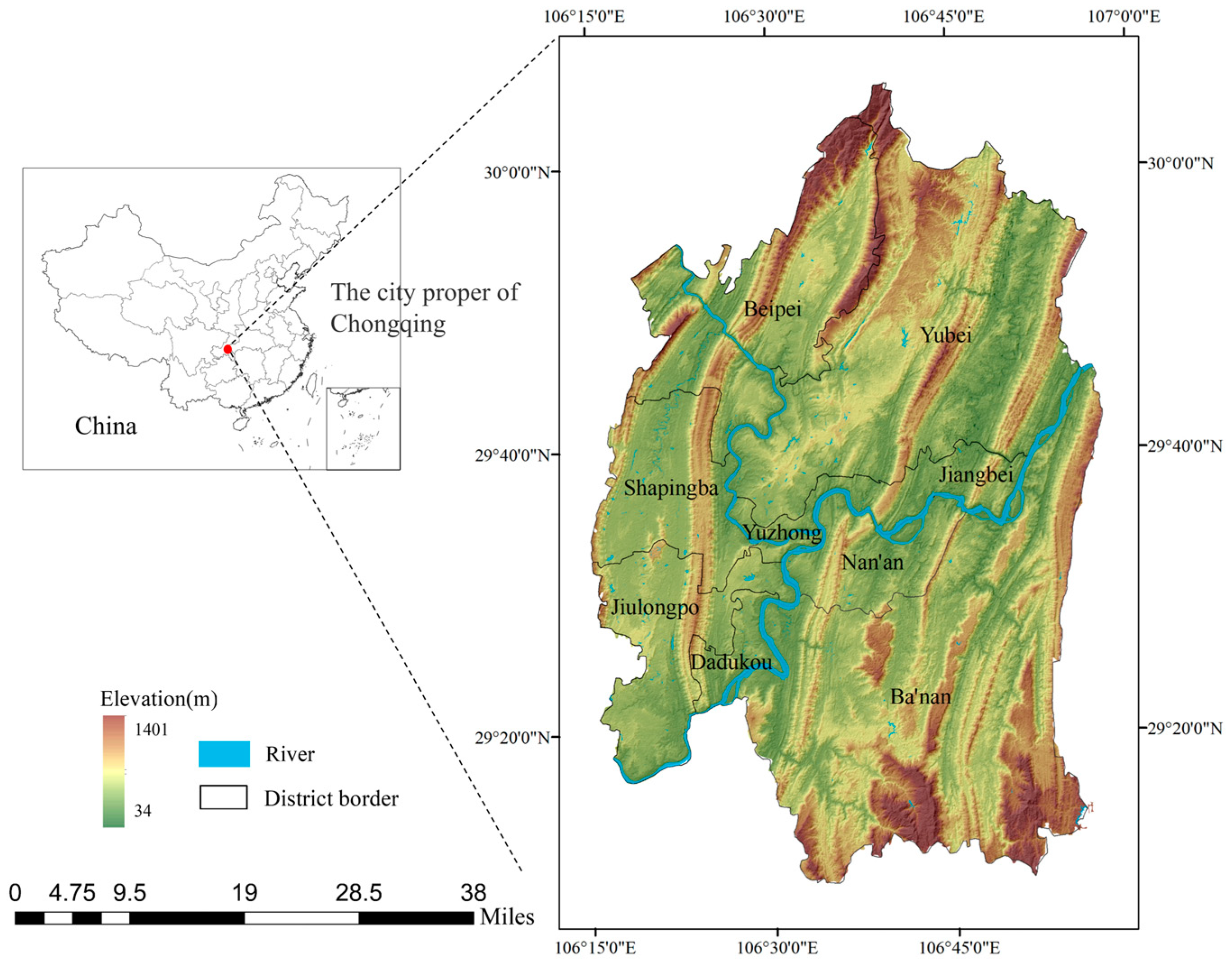
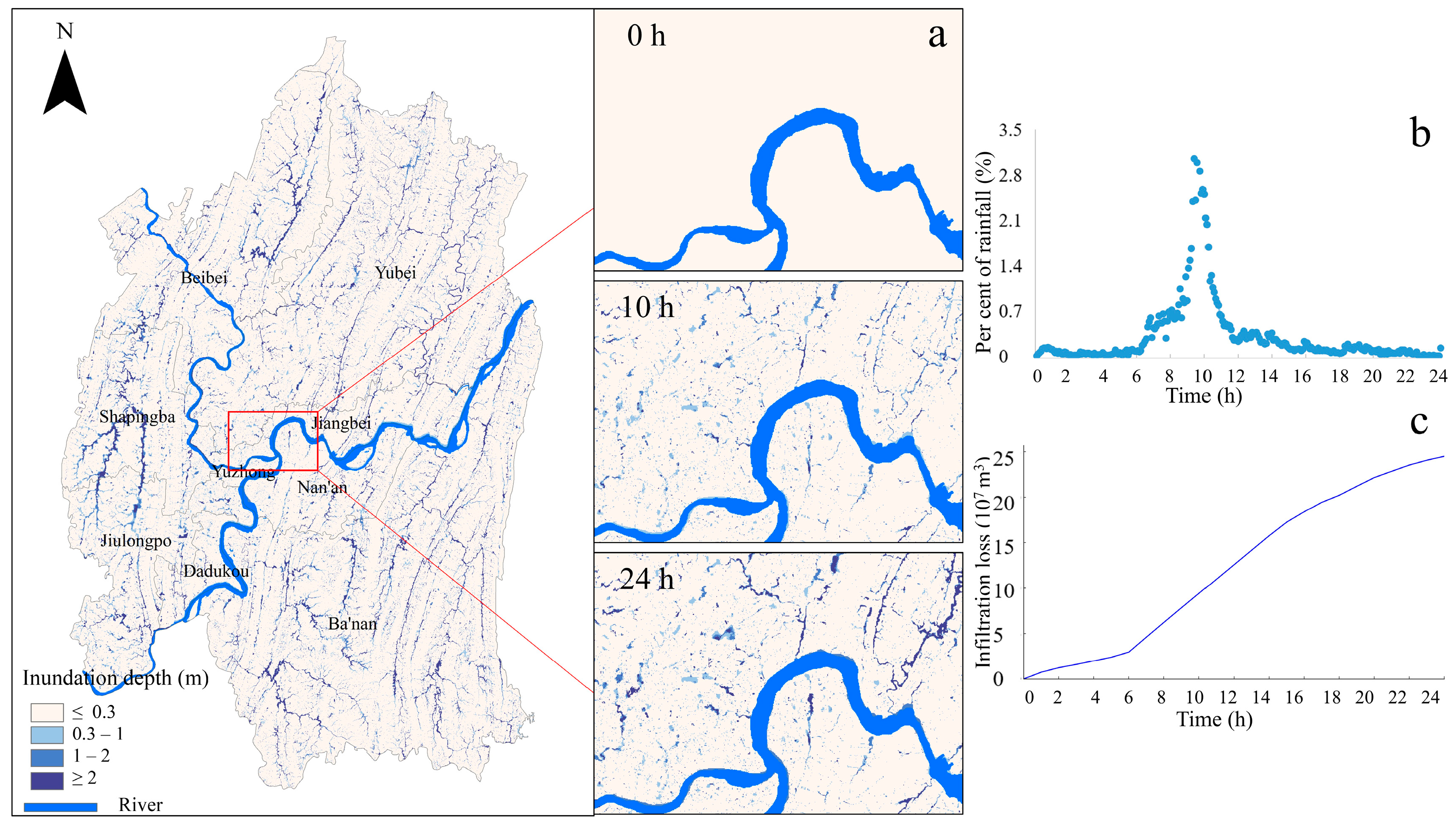
2. Study Area
3. Data and Methods
3.1. Data Sources
3.2. Methods
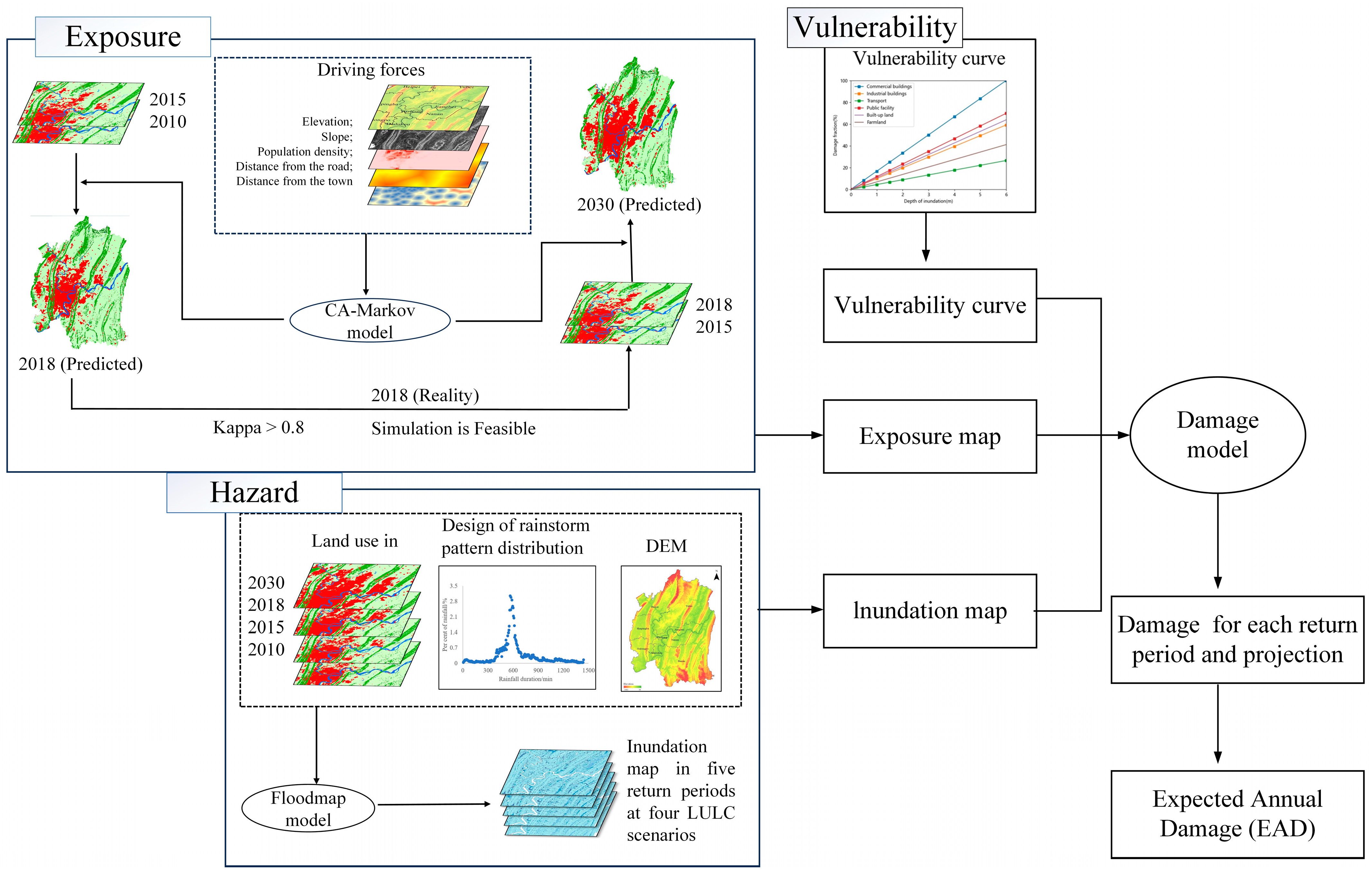
3.2.1. Flood Exposure and Vulnerability Analysis
Flood Exposure
- (1)
- Determining the transition rules
- (2)
- Determining CA filters and the number of iterations
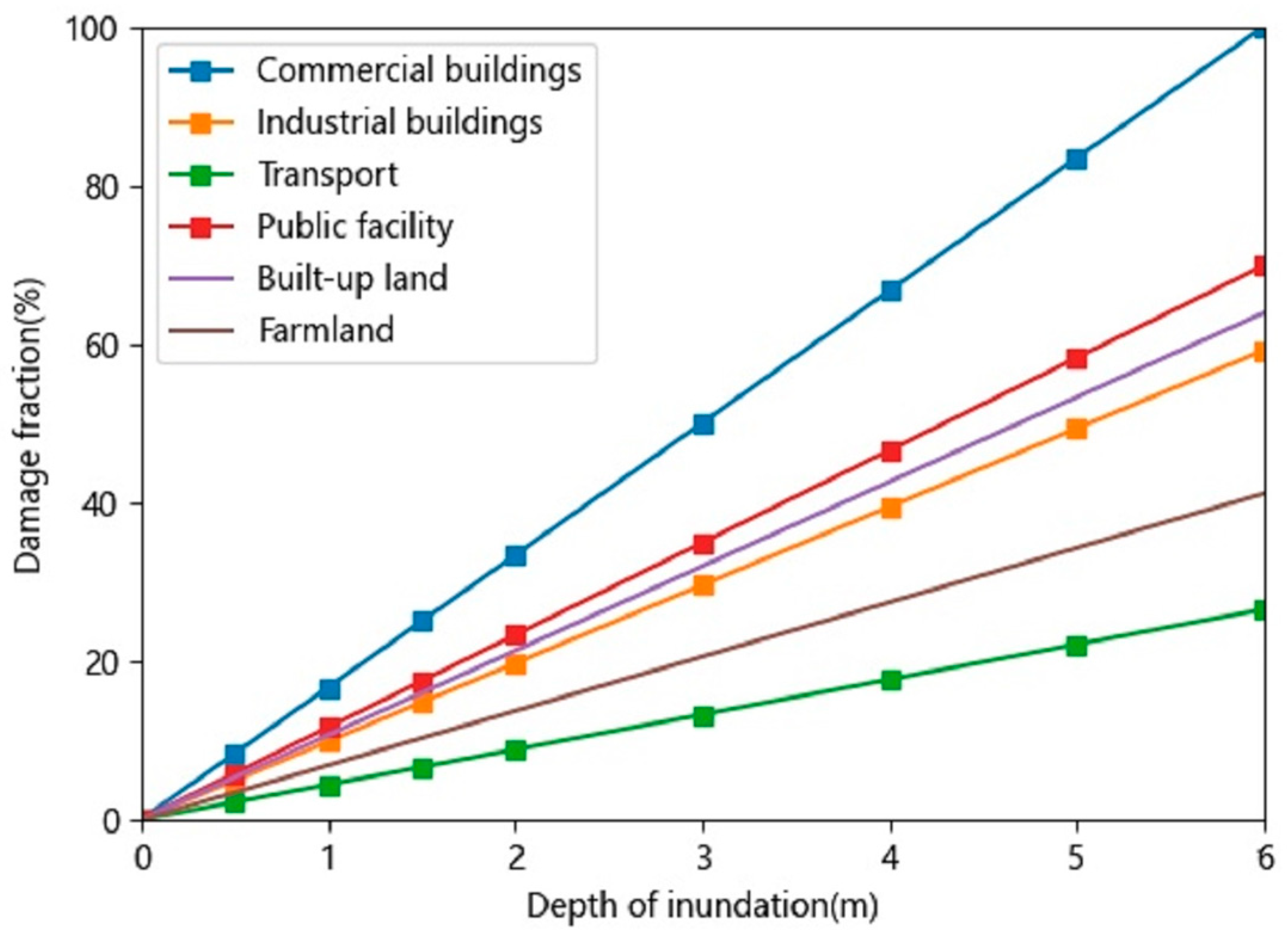
Flood Vulnerability
3.2.2. Flood Inundation Analysis
3.2.3. Flood Risk Assessment
4. Results
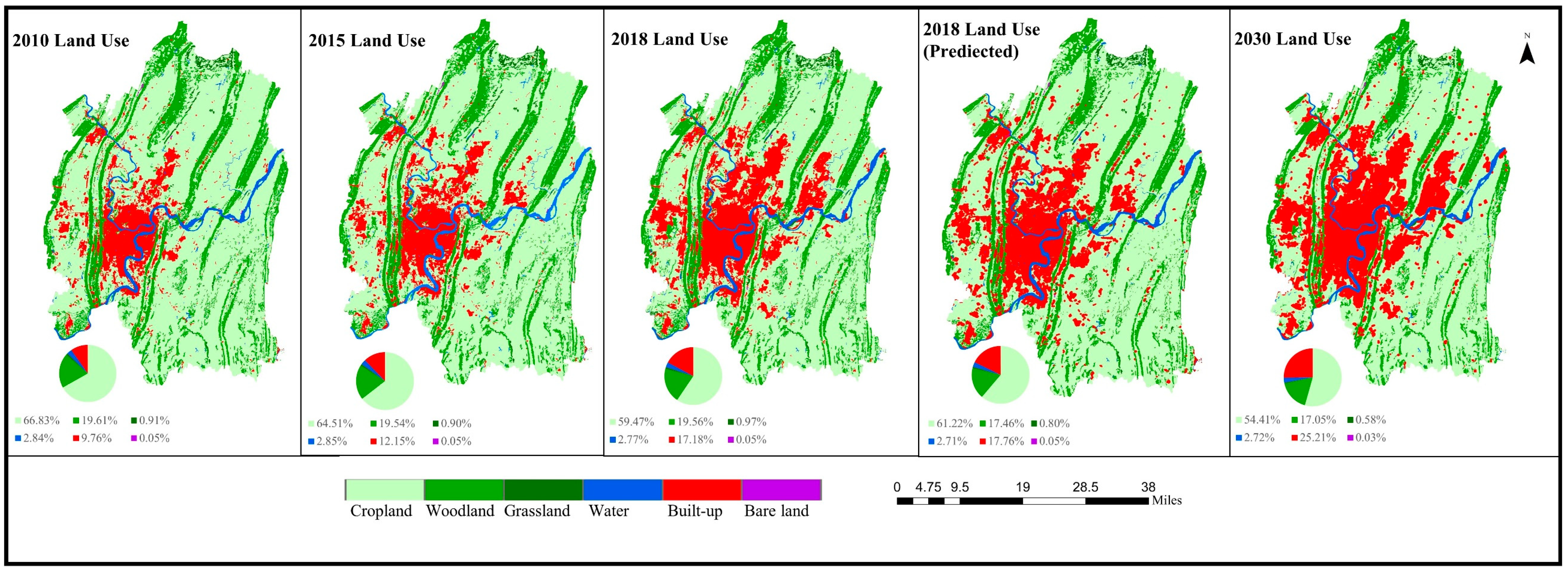
4.1. The Temporal and Spatial Changes in LULC
4.2. The Impacts of Urbanization Changes on Flood Risk
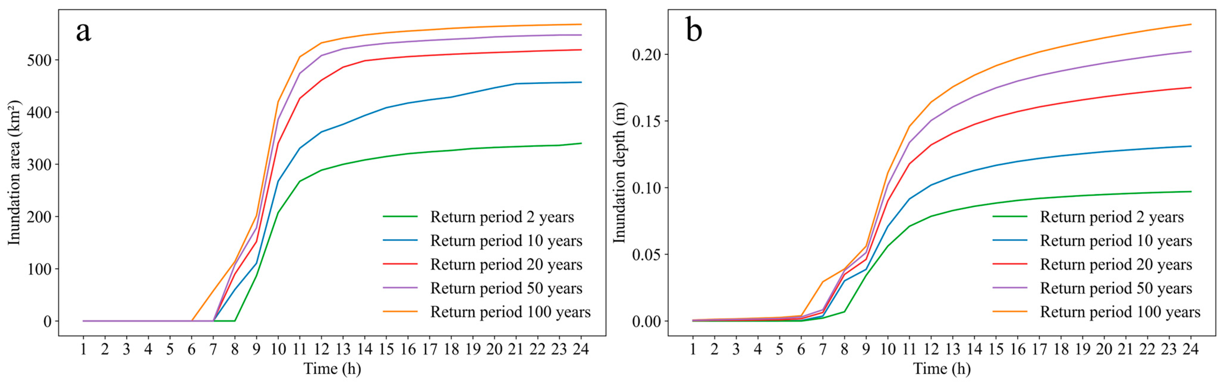
4.2.1. Flood Damage
4.2.2. Flood Risk
4.2.3. The Association of Flood Risk Factors Analysis
5. Discussion
6. Conclusions
Supplementary Materials
Author Contributions
Funding
Data Availability Statement
Acknowledgments
Conflicts of Interest
References
- IPCC. Climate Change 2021: The Physical Science Basis. Contribution of Working Group I to the Sixth Assessment Report of the Intergovernmental Panel on Climate Change; Cambridge University Press: Cambridge, UK; New York, NY, USA, 2021; p. 2391. [Google Scholar]
- Marsooli, R.; Lin, N.; Emanuel, K.; Feng, K. Climate change exacerbates hurricane flood hazards along US Atlantic and Gulf Coasts in spatially varying patterns. Nat. Commun. 2019, 10, 3785. [Google Scholar] [CrossRef] [PubMed]
- United Nations Office for Disaster Risk Reduction (UNISDR) & Centre for Research on the Epidemiology of Disasters (CRED). The Human Cost of Natural Disasters: A Global Perspective. Available online: https://reliefweb.int/report/world/human-cost-natural-disasters-2015-global-perspective (accessed on 22 May 2022).
- He, B.; Huang, X.; Ma, M.; Chang, Q.; Tu, Y.; Li, Q.; Zhang, K.; Hong, Y. Analysis of flash flood disaster characteristics in China from 2011 to 2015. Nat. Hazards 2018, 90, 407–420. [Google Scholar] [CrossRef]
- EM-DAT. The OFDA/CRED International Disaster Database. Available online: https://www.emdat.be/ (accessed on 22 May 2022).
- Xiao, Y.; Yi, S.; Tang, Z. A Spatially Explicit Multi-Criteria Analysis Method on Solving Spatial Heterogeneity Problems for Flood Hazard Assessment. Water Resour. Manag. 2018, 32, 3317–3335. [Google Scholar] [CrossRef]
- Deng, Z.; Wang, Z.; Wu, X.; Lai, C.; Zeng, Z. Strengthened tropical cyclones and higher flood risk under compound effect of climate change and urbanization across China’s Greater Bay Area. Urban Clim. 2022, 44, 101224. [Google Scholar] [CrossRef]
- Zhao, J.; Chen, H.; Liang, Q.; Xia, X.; Xu, J.; Hoey, T.; Barrett, B.; Renaud, F.G.; Bosher, L.; Zhou, X. Large-scale flood risk assessment under different development strategies: The Luanhe River Basin in China. Sustain. Sci. 2022, 17, 1365–1384. [Google Scholar] [CrossRef]
- Guoyi, L.; Liu, J.; Shao, W. Urban flood risk assessment under rapid urbanization in Zhengzhou City, China. Reg. Sustain. 2023, 4, 332–348. [Google Scholar] [CrossRef]
- Yu, I.; Jung, H. Flood Risk Assessment to Enable Improved Decision-Making for Climate Change Adaptation Strategies by Central and Local Governments. Sustainability 2022, 14, 14335. [Google Scholar] [CrossRef]
- Baky, M.A.A.; Islam, M.; Paul, S. Flood Hazard, Vulnerability and Risk Assessment for Different Land Use Classes Using a Flow Model. Earth Syst. Environ. 2020, 4, 225–244. [Google Scholar] [CrossRef]
- Schwarz, I.; Kuleshov, Y. Flood Vulnerability Assessment and Mapping: A Case Study for Australia’s Hawkesbury-Nepean Catchment. Remote Sens. 2022, 14, 4894. [Google Scholar]
- Wu, S.; Liu, L.; Gao, J.; Wang, W. Integrate Risk From Climate Change in China Under Global Warming of 1.5 and 2.0 °C. Earth’s Future 2019, 7, 1307–1322. [Google Scholar] [CrossRef]
- Koks, E.E.; Jongman, B.; Husby, T.G.; Botzen, W.J.W. Combining hazard, exposure and social vulnerability to provide lessons for flood risk management. Environ. Sci. Policy 2015, 47, 42–52. [Google Scholar] [CrossRef]
- Güneralp, B.; Güneralp, İ.; Liu, Y. Changing global patterns of urban exposure to flood and drought hazards. Glob. Environ. Chang. 2015, 31, 217–225. [Google Scholar] [CrossRef]
- Garg, V.; Aggarwal, S.; Gupta, P.K.; Nikam, B.R.; Thakur, P.K.; Srivastav, S.; Senthil Kumar, A. Assessment of land use land cover change impact on hydrological regime of a basin. Environ. Earth Sci. 2017, 76, 635. [Google Scholar] [CrossRef]
- Hemmati, M.; Ellingwood, B.R.; Mahmoud, H.N. The role of urban growth in resilience of communities under flood risk. Earth’s Future 2020, 8, e2019EF001382. [Google Scholar] [CrossRef] [PubMed]
- Mandarino, A.; Faccini, F.; Luino, F.; Bono, B.; Turconi, L. Integrated Approach for the Study of Urban Expansion and River Floods Aimed at Hydrogeomorphic Risk Reduction. Remote Sens. 2023, 15, 4158. [Google Scholar] [CrossRef]
- Cai, J.; Li, X.; Liu, L.; Chen, Y.; Wang, X.; Lu, S. Coupling and coordinated development of new urbanization and agro-ecological environment in China. Sci. Total Environ. 2021, 776, 145837. [Google Scholar] [CrossRef]
- Mechler, R.; Bouwer, L.M.; Linnerooth-Bayer, J.; Hochrainer-Stigler, S.; Aerts, J.C.; Surminski, S.; Williges, K. Managing unnatural disaster risk from climate extremes. Nat. Clim. Chang. 2014, 4, 235–237. [Google Scholar] [CrossRef]
- Broderick, C.; Murphy, C.; Wilby, R.L.; Matthews, T.; Prudhomme, C.; Adamson, M. Using a scenario-neutral framework to avoid potential maladaptation to future flood risk. Water Resour. Res. 2019, 55, 1079–1104. [Google Scholar] [CrossRef]
- Zhou, Q.; Leng, G.; Su, J.; Ren, Y. Comparison of urbanization and climate change impacts on urban flood volumes: Importance of urban planning and drainage adaptation. Sci. Total Environ. 2019, 658, 24–33. [Google Scholar] [CrossRef]
- Xu, H.; Tian, Z.; Sun, L.; Ye, Q.; Ragno, E.; Bricker, J.; Mao, G.; Tan, J.; Wang, J.; Ke, Q. Compound flood impact of water level and rainfall during tropical cyclone periods in a coastal city: The case of Shanghai. Nat. Hazards Earth Syst. 2022, 22, 2347–2358. [Google Scholar] [CrossRef]
- Dada, O.A.; Almar, R.; Morand, P.; Bergsma, E.W.J.; Angnuureng, D.B.; Minderhoud, P.S.J. Future socioeconomic development along the West African coast forms a larger hazard than sea level rise. Commun. Earth Environ. 2023, 4, 150. [Google Scholar] [CrossRef]
- Tang, J.; Li, W.; Fang, J.; Zhang, Z.; Du, S.; Wu, Y.; Wen, J. Scenario-based economic and societal risk assessment of storm flooding in Shanghai. Int. J. Clim. Chang. Strat. Manag. 2021, 13, 529–546. [Google Scholar] [CrossRef]
- Kang, S.; Yin, J.; Gu, L.; Yang, Y.; Liu, D.; Slater, L. Observation-Constrained Projection of Flood Risks and Socioeconomic Exposure in China. Earth’s Future 2023, 11, e2022EF003308. [Google Scholar] [CrossRef]
- Zhou, N.; Sheng, S.; He, L.-Y.; Tian, B.-R.; Chen, H.; Xu, C.-Y. An Integrated Approach for Analyzing the Morphological Evolution of the Lower Reaches of the Minjiang River Based on Long-Term Remote Sensing Data. Remote Sens. 2023, 15, 3093. [Google Scholar] [CrossRef]
- Huang, W.; Liu, H.; Luan, Q.; Jiang, Q.; Liu, J.; Liu, H. Detection and prediction of land use change in Beijing based on remote sensing and GIS. Int. Arch. Photogramm. Remote Sens. Spat. Inf. Sci. 2008, 37, 75–82. [Google Scholar]
- Lin, W.; Sun, Y.; Nijhuis, S.; Wang, Z. Scenario-based flood risk assessment for urbanizing deltas using future land-use simulation (FLUS): Guangzhou Metropolitan Area as a case study. Sci. Total Environ. 2020, 739, 139899. [Google Scholar] [CrossRef] [PubMed]
- Muis, S.; Güneralp, B.; Jongman, B.; Aerts, J.C.; Ward, P.J. Flood risk and adaptation strategies under climate change and urban expansion: A probabilistic analysis using global data. Sci. Total Environ. 2015, 538, 445–457. [Google Scholar] [CrossRef]
- Mustafa, A.; Bruwier, M.; Archambeau, P.; Erpicum, S.; Pirotton, M.; Dewals, B.; Teller, J. Effects of spatial planning on future flood risks in urban environments. J. Environ. Manag. 2018, 225, 193–204. [Google Scholar] [CrossRef]
- Sang, L.; Zhang, C.; Yang, J.; Zhu, D.; Yun, W. Simulation of land use spatial pattern of towns and villages based on CA–Markov model. Math. Comput. Model. 2011, 54, 938–943. [Google Scholar] [CrossRef]
- Fu, X.; Wang, X.; Yang, Y.J. Deriving suitability factors for CA-Markov land use simulation model based on local historical data. J. Environ. Manag. 2018, 206, 10–19. [Google Scholar] [CrossRef]
- Zhang, C.-X.; Xu, J.-J.; Wen, J.; Yang, X.-B.; Wang, J.; Zhao, B. Dynamic simulation of landscape change in the Baiyangdian basin based on the CA-Markov model and MCE constraints. J. Agric. Resour. Environ. 2021, 38, 655–664. [Google Scholar]
- Kindu, M.; Schneider, T.; Döllerer, M.; Teketay, D.; Knoke, T. Scenario modelling of land use/land cover changes in Munessa-Shashemene landscape of the Ethiopian highlands. Sci. Total Environ. 2018, 622–623, 534–546. [Google Scholar] [CrossRef] [PubMed]
- Nkwunonwo, U.C.; Whitworth, M.; Baily, B. A review of the current status of flood modelling for urban flood risk management in the developing countries. Sci. Afr. 2020, 7, e00269. [Google Scholar] [CrossRef]
- Bulti, D.T.; Abebe, B.G. A review of flood modeling methods for urban pluvial flood application. Model. Earth Syst. Environ. 2020, 6, 1293–1302. [Google Scholar] [CrossRef]
- Bates, P.D.; Horritt, M.S.; Fewtrell, T.J. A simple inertial formulation of the shallow water equations for efficient two-dimensional flood inundation modelling. J. Hydrol. 2010, 387, 33–45. [Google Scholar] [CrossRef]
- Teng, J.; Jakeman, A.J.; Vaze, J.; Croke, B.F.; Dutta, D.; Kim, S. Flood inundation modelling: A review of methods, recent advances and uncertainty analysis. Environ. Model. Softw. 2017, 90, 201–216. [Google Scholar] [CrossRef]
- Yu, D.; Lane, S.N. Urban fluvial flood modelling using a two-dimensional diffusion-wave treatment, part 2: Development of a sub-grid-scale treatment. Hydrol. Process. 2006, 20, 1567–1583. [Google Scholar] [CrossRef]
- Yu, D.; Lane, S.N. Urban fluvial flood modelling using a two-dimensional diffusion-wave treatment, part 1: Mesh resolution effects. Hydrol. Process. 2006, 20, 1541–1565. [Google Scholar] [CrossRef]
- Bradbrook, K. JFLOW: A multiscale two-dimensional dynamic flood model. Water Environ. J. 2006, 20, 79–86. [Google Scholar] [CrossRef]
- Yu, D.; Coulthard, T.J. Evaluating the importance of catchment hydrological parameters for urban surface water flood modelling using a simple hydro-inundation model. J. Hydrol. 2015, 524, 385–400. [Google Scholar] [CrossRef]
- Hawker, L.; Uhe, P.; Paulo, L.; Sosa, J.; Savage, J.; Sampson, C.; Neal, J. A 30 m global map of elevation with forests and buildings removed. Environ. Res. Lett. 2022, 17, 024016. [Google Scholar] [CrossRef]
- Fu, Y.; Wang, Z. A Study of County’s Economic Group Development Model in Chongqing. Stud. Sociol. Sci. 2015, 6, 63. [Google Scholar]
- Li, Q.; Zheng, Y.; Zhou, G.; Zhu, Y.; Liu, C.; Liu, Y. Diurnal variations of rainfall affected by complex topography based on high-density observation in Chongqing over southwest China. Theor. Appl. Climatol. 2022, 148, 1373–1394. [Google Scholar] [CrossRef]
- Qianzhu, Z.; Huoming, Z.; Yang, L.; Ruiyi, Z.; Qiang, G.; Jianmei, Y.; Kun, S. Research on chongqing mountain flood disaster risk assessment system based on AHP-GIS. In IOP Conference Series: Earth and Environmental Science; IOP Publishing: Bristol, UK, 2019; p. 032028. [Google Scholar]
- Jiao, M.Y. China Meteorological Disaster Yearbook; China Meteorological Press: Beijing, China, 2019; pp. 86–157. [Google Scholar]
- Chongqing Housing and Urban-Rural Development Commission. Information on the Publication of the Revised Formulae for Storm Intensity and the Design of Storm Rain Patterns in Chongqing. Available online: https://zfcxjw.cq.gov.cn/zwxx_166/gsgg/201708/t20170823_4216173.html (accessed on 10 August 2022).
- Mansour, S.; Al-Belushi, M.; Al-Awadhi, T. Monitoring land use and land cover changes in the mountainous cities of Oman using GIS and CA-Markov modelling techniques. Land Use Policy 2020, 91, 104414. [Google Scholar] [CrossRef]
- Liu, J.; Tian, Y.; Tian, L.; Zhang, X.; Wan, Z.; Liu, X. A Comparative Study on Planning Constraints of the Rapid Urbanization Area Expansion Simulation. Geogr. Geo-Inform. Sci. 2019, 35, 82–88. [Google Scholar]
- Mondal, M.S.; Sharma, N.; Garg, P.K.; Kappas, M. Statistical independence test and validation of CA Markov land use land cover (LULC) prediction results. Egypt. J. Remote Sens. Space Sci. 2016, 19, 259–272. [Google Scholar] [CrossRef]
- Yu, L.; Li, M.; Wang, S.; Zhao, Y. Wetland landscape change in Daliaohe River basin and the driving factors analysis. Procedia Environ. Sci. 2010, 2, 1255–1264. [Google Scholar] [CrossRef][Green Version]
- Yin, J. Study on the Risk Assessment of Typhoon Strom Tide in China Coastal Area. Ph.D. Thesis, East China Normal University, Shanghai, China, 2011. [Google Scholar]
- Moel, H.; Huizinga, J.; Szewczyk, W. Global Flood Depth-Damage Functions—Methodology and the Database with Guidelines; European Commission, Joint Research Centre: Sevilla, Spain, 2016; pp. 35–56. [Google Scholar]
- Feng, A. Change and Disaster Risk of Extreme Water Levels under Sea-Level Rise Scenarios in Coastal Region, Shandong. Ph.D. Thesis, Institute of Geographic Sciences and Natural Resources Research, Chinese Academy of Sciences, Beijing, China, 2017. [Google Scholar]
- Liu, L.; Xu, Z.X. Regionalization of precipitation and the spatiotemporal distribution of extreme precipitation in southwestern China. Nat. Hazards 2016, 80, 1195–1211. [Google Scholar] [CrossRef]
- Yin, J.; Yu, D.; Yin, Z.; Wang, J.; Xu, S. Modelling the anthropogenic impacts on fluvial flood risks in a coastal mega-city: A scenario-based case study in Shanghai, China. Landsc. Urban Plan. 2015, 136, 144–155. [Google Scholar] [CrossRef]
- Yin, J.; Yu, D.; Lin, N.; Wilby, R.L. Evaluating the cascading impacts of sea level rise and coastal flooding on emergency response spatial accessibility in Lower Manhattan, New York City. J. Hydrol. 2017, 555, 648–658. [Google Scholar] [CrossRef]
- Peng, J.; Wei, H.; Wu, W.H.; Liu, Y.X.; Wang, Y. Storm flood disaster risk assessment in urban area based on the simulation of land use scenarios: A case of Maozhou Watershed in Shenzhen City. Acta Ecol. Sin. 2018, 38, 3741–3755. [Google Scholar]
- Hammond, M.J.; Chen, A.S.; Djordjević, S.; Butler, D.; Mark, O. Urban flood impact assessment: A state-of-the-art review. Urban Water J. 2015, 12, 14–29. [Google Scholar] [CrossRef]
- Islam, M.F.; Bhattacharya, B.; Popescu, I. Flood risk assessment due to cyclone-induced dike breaching in coastal areas of Bangladesh. Nat. Hazards Earth Syst. 2019, 19, 353–368. [Google Scholar] [CrossRef]
- Zhang, W.; Villarini, G.; Vecchi, G.A.; Smith, J.A. Urbanization exacerbated the rainfall and flooding caused by hurricane Harvey in Houston. Nature 2018, 563, 384–388. [Google Scholar] [CrossRef] [PubMed]
- Shi, J.; Cui, L.; Ma, Y.; Du, H.; Wen, K. Trends in temperature extremes and their association with circulation patterns in China during 1961–2015. Atmos. Res. 2018, 212, 259–272. [Google Scholar] [CrossRef]
- Jongman, B.; Ward, P.J.; Aerts, J.C. Global exposure to river and coastal flooding: Long term trends and changes. Glob. Environ. Chang. 2012, 22, 823–835. [Google Scholar] [CrossRef]
- Liao, G.; He, P.; Gao, X.; Deng, L.; Zhang, H.; Feng, N.; Zhou, W.; Deng, O. The Production–Living–Ecological Land Classification System and Its Characteristics in the Hilly Area of Sichuan Province, Southwest China Based on Identification of the Main Functions. Sustainability 2019, 11, 1600. [Google Scholar] [CrossRef]
- Ouma, Y.O.; Tateishi, R. Urban flood vulnerability and risk mapping using integrated multi-parametric AHP and GIS: Methodological overview and case study assessment. Water 2014, 6, 1515–1545. [Google Scholar] [CrossRef]
- Wang, X.; Xia, J.; Dong, B.; Zhou, M.; Deng, S. Spatiotemporal distribution of flood disasters in Asia and influencing factors in 1980–2019. Nat. Hazards 2021, 108, 2721–2738. [Google Scholar] [CrossRef]
- Li, C.; Chai, Y.; Yang, L.; Li, H. Spatio-temporal distribution of flood disasters and analysis of influencing factors in Africa. Nat. Hazards 2016, 82, 721–731. [Google Scholar] [CrossRef]
- Ju, H.; Zhang, Z.; Zhao, X.; Wang, X.; Wu, W.; Yi, L.; Wen, Q.; Liu, F.; Xu, J.; Hu, S. The changing patterns of cropland conversion to built-up land in China from 1987 to 2010. J. Geogr. Sci. 2018, 28, 1595–1610. [Google Scholar] [CrossRef]
- Zuo, Y.; Cheng, J.; Fu, M. Analysis of Land Use Change and the Role of Policy Dimensions in Ecologically Complex Areas: A Case Study in Chongqing. Land 2022, 11, 627. [Google Scholar] [CrossRef]
- Szwagrzyk, M.; Kaim, D.; Price, B.; Wypych, A.; Grabska, E.; Kozak, J. Impact of forecasted land use changes on flood risk in the Polish Carpathians. Nat. Hazards 2018, 94, 227–240. [Google Scholar] [CrossRef]
- Aguejdad, R. The Influence of the Calibration Interval on Simulating Non-Stationary Urban Growth Dynamic Using CA-Markov Model. Remote Sens. 2021, 13, 468. [Google Scholar] [CrossRef]
- Cole, S.J.; Moore, R.J. Hydrological modelling using raingauge- and radar-based estimators of areal rainfall. J. Hydrol. 2008, 358, 159–181. [Google Scholar] [CrossRef]
- Adnan, M.S.G.; Abdullah, A.Y.M.; Dewan, A.; Hall, J.W. The effects of changing land use and flood hazard on poverty in coastal Bangladesh. Land Use Policy 2020, 99, 104868. [Google Scholar] [CrossRef]
- Winsemius, H.C.; Jongman, B.; Veldkamp, T.I.; Hallegatte, S.; Bangalore, M.; Ward, P.J. Disaster risk, climate change, and poverty: Assessing the global exposure of poor people to floods and droughts. Environ. Dev. Econ. 2018, 23, 328–348. [Google Scholar] [CrossRef]
- Kawasaki, A.; Kawamura, G.; Zin, W.W. A local level relationship between floods and poverty: A case in Myanmar. Int. J. Disaster Risk Reduct. 2020, 42, 101348. [Google Scholar] [CrossRef]


| Cropland | Woodland | Grassland | Water | Built-Up Land | Bare Land | Transfer Out | |
|---|---|---|---|---|---|---|---|
| Cropland | 3513.6 | 7.7 | 0.6 | 1.2 | 129.0 | 0.0 | 138.6 |
| Woodland | 7.8 | 1059.2 | 0.1 | 0.1 | 4.6 | 0.0 | 12.6 |
| Grassland | 0.6 | 0.1 | 48.6 | 0.3 | 0.2 | 0.0 | 1.1 |
| Water | 0.8 | 0.1 | 0.0 | 153.6 | 0.4 | 0.0 | 1.4 |
| Built-up land | 2.5 | 0.5 | 0.0 | 0.2 | 530.0 | 0.0 | 3.3 |
| Bare land | 0.0 | 0.0 | 0.0 | 0.0 | 0.0 | 2.8 | 0.0 |
| Transfer in | 11.8 | 8.5 | 0.7 | 2.0 | 134.1 | 0.0 | 157.0 |
| Net transfer out | 126.8 | 4.1 | 0.5 | −0.6 | −130.8 | 0.0 | 0 |
| Cropland | Woodland | Grassland | Water | Built-Up Land | Bare Land | ||
|---|---|---|---|---|---|---|---|
| 2010–2015 | Change of area (km2) | −126.77 | −4.13 | −0.50 | 0.58 | 130.83 | −0.01 |
| Dynamic attitude/% | −0.69% | −0.08% | −0.20% | 0.08% | 4.91% | −0.09% | |
| 2015–2018 | Change of area (km2) | −275.35 | 1.09 | 4.06 | −4.28 | 274.45 | 0.02 |
| Dynamic attitude/% | −2.60% | 0.03% | 2.75% | −0.92% | 13.77% | 0.19% | |
| 2018–2030 | Change of area (km2) | −276.74 | −136.86 | −21.91 | −2.56 | 439.16 | −1.07 |
| Dynamic attitude/% | −0.71% | −1.07% | −3.42% | −0.14% | 3.90% | −3.15% |
| ID | 2010 (km²) | 2015 (km²) | 2018 (km²) | 2030 (km²) |
|---|---|---|---|---|
| Very low | 474.52 | 595.49 | 838.16 | 1228.11 |
| Low | 32.68 | 37.30 | 50.46 | 301.61 |
| Medium | 14.0 | 16.40 | 24.01 | 147.23 |
| High | 11.96 | 14.80 | 25.80 | 178.21 |
| Flood Risk | |
|---|---|
| SEI | −0.057 * |
| LULC | 0.095 ** |
| Population-density | 0.049 ** |
| DEM | −0.097 ** |
| Slope | −0.112 ** |
Disclaimer/Publisher’s Note: The statements, opinions and data contained in all publications are solely those of the individual author(s) and contributor(s) and not of MDPI and/or the editor(s). MDPI and/or the editor(s) disclaim responsibility for any injury to people or property resulting from any ideas, methods, instructions or products referred to in the content. |
© 2024 by the authors. Licensee MDPI, Basel, Switzerland. This article is an open access article distributed under the terms and conditions of the Creative Commons Attribution (CC BY) license (https://creativecommons.org/licenses/by/4.0/).
Share and Cite
Li, Y.; Gao, J.; Yin, J.; Liu, L.; Zhang, C.; Wu, S. Flood Risk Assessment of Areas under Urbanization in Chongqing, China, by Integrating Multi-Models. Remote Sens. 2024, 16, 219. https://doi.org/10.3390/rs16020219
Li Y, Gao J, Yin J, Liu L, Zhang C, Wu S. Flood Risk Assessment of Areas under Urbanization in Chongqing, China, by Integrating Multi-Models. Remote Sensing. 2024; 16(2):219. https://doi.org/10.3390/rs16020219
Chicago/Turabian StyleLi, Yuqing, Jiangbo Gao, Jie Yin, Lulu Liu, Chuanwei Zhang, and Shaohong Wu. 2024. "Flood Risk Assessment of Areas under Urbanization in Chongqing, China, by Integrating Multi-Models" Remote Sensing 16, no. 2: 219. https://doi.org/10.3390/rs16020219
APA StyleLi, Y., Gao, J., Yin, J., Liu, L., Zhang, C., & Wu, S. (2024). Flood Risk Assessment of Areas under Urbanization in Chongqing, China, by Integrating Multi-Models. Remote Sensing, 16(2), 219. https://doi.org/10.3390/rs16020219