Article

High-Precision Heterogeneous Satellite Image Manipulation Localization: Feature Point Rules and Semantic Similarity Measurement

1
State Key Laboratory of Information Engineering in Surveying, Mapping, and Remote Sensing, Wuhan University, Wuhan 430079, China
2
School of Geodesy and Geomatics, Wuhan University, Wuhan 430079, China
*
Author to whom correspondence should be addressed.
Remote Sens. 2024, 16(19), 3719; https://doi.org/10.3390/rs16193719
Submission received: 5 September 2024 / Revised: 26 September 2024 / Accepted: 1 October 2024 / Published: 6 October 2024

Abstract

:
Misusing image tampering software makes it easier to manipulate satellite images, leading to a crisis of trust and security concerns in society. This study compares the inconsistencies between heterogeneous images to locate tampered areas and proposes a high-precision heterogeneous satellite image manipulation localization (HSIML) framework to distinguish tampered from real landcover changes, such as artificial constructions, and pseudo-changes, such as seasonal variations. The model operates at the patch level and comprises three modules: The heterogeneous image preprocessing module aligns heterogeneous images and filters noisy data. The feature point constraint module mitigates the effects of lighting and seasonal variations in the images by performing feature point matching, applying filtering rules to conduct an initial screening to identify candidate tampered patches. The semantic similarity measurement module designs a classification network to assess RS image feature saliency. It determines image consistency based on the similarity of semantic features and implements IML using predefined classification rules. Additionally, a dataset for IML is constructed based on satellite images. Extensive experiments compared with existing SOTA models demonstrate that our method achieved the highest F1 score in both localization accuracy and robustness tests and demonstrates the capability for handling large-scale areas.

1. Introduction

The widespread application of remote sensing (RS) technology has enabled the public to easily access RS image data from open sources and apply it across various fields, such as urban expansion [1,2,3], scene classification [4,5], and land use detection [6,7,8]. However, with the continuous development of image editing software and deep learning, it has become easy for individuals to modify natural images, including satellite images, leading to significant trust issues and security risks for the public [9].
Current mainstream image manipulation localization (IML) methods focus primarily on natural images, performing pixel-level detection for common tampering techniques such as copy-move, splicing, and inpainting [10]. These methods work by locating the edge artifacts of tampered regions and training models to learn the distribution of these edges. However, these methods are not entirely applicable to RS imagery. As shown in Figure 1, examples of three tampering methods in RS imagery illustrate several challenges. Firstly, the acquisition methods for RS images differ significantly from those of natural images including sensor types, spectral channels, and post-processing techniques. For example, forests may appear lush green in summer but reveal more bare ground in winter. Similarly, the same area may exhibit different spectral characteristics due to variations in spectral reflectance. Secondly, RS images encompass diverse types of terrain and objects. Tampering artifacts at edges in mountainous or forested areas, for instance, can be easily masked by the natural textures of the terrain itself, increasing the difficulty in accurately locating edges.
Research on RSIML remains limited: the primary detection principle involves training networks to learn the distribution [11] and mapping relationships of objects [12,13] in remote sensing imagery, identifying regions with inconsistent distributions within a single image. However, these methods still face unresolved challenges and opportunity within RSIML.
(1) Existing studies focus predominantly on detecting conspicuous tampering techniques such as splicing in Figure 1, which has clearly boundaries and significant conflicts in object distributions, thus being relatively easier to detect. In contrast, the other two tampering methods exhibit greater concealment, seamlessly blending altered content with the scene and lacking obvious conflicts in object distributions, making them challenging to pinpoint using current detection strategies.
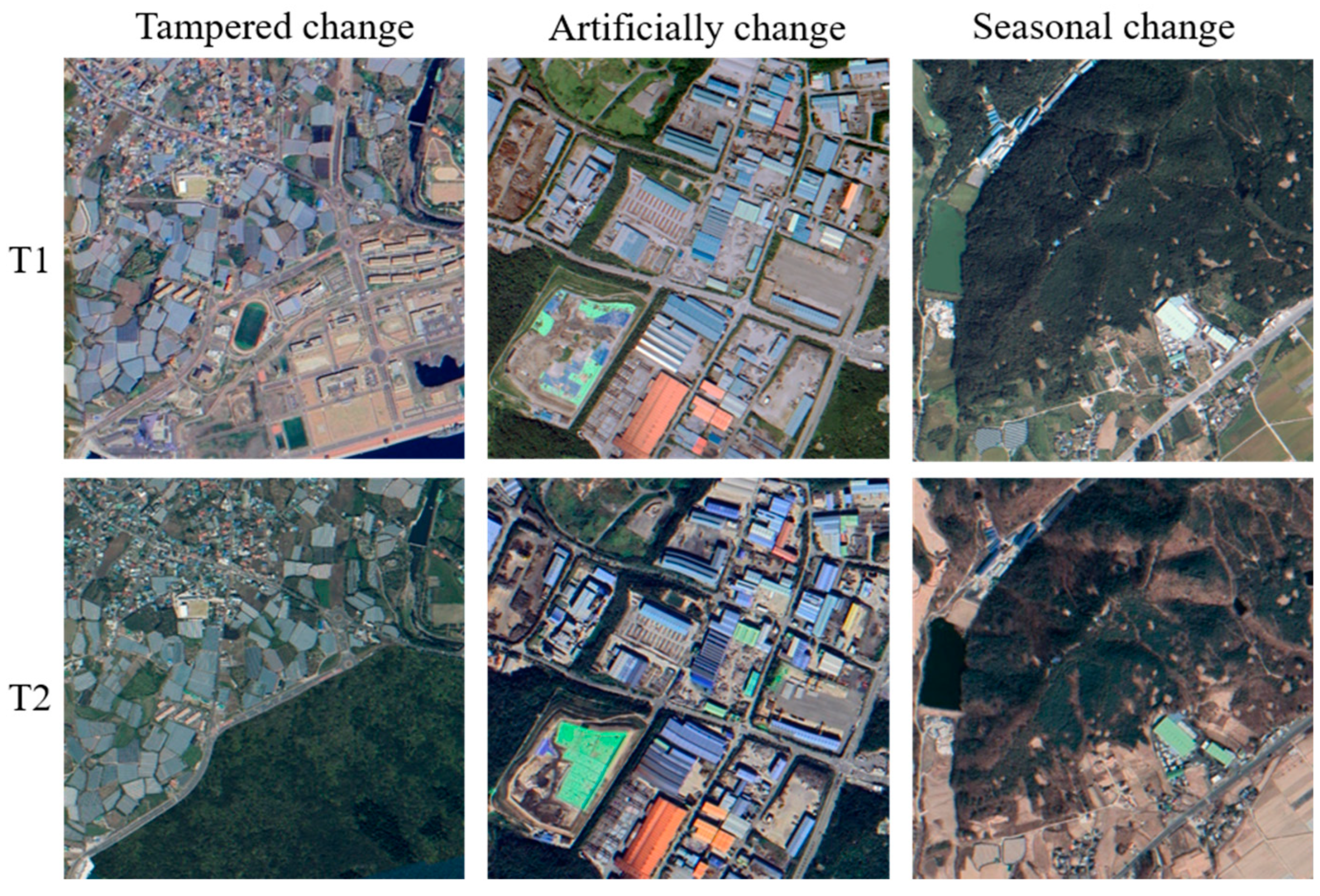
(2) Current research has focused on detecting tampered regions directly from single-source images, neglecting the significant presence of distributional consistency across multiple sources. Integrating heterogeneous images can thus be used to enhance mutual verification. However, it is worth noting that heterogeneous images cannot be directly aligned. For example, the Google Map, Tianditu, and Yandex Map services come from different countries, and their reference coordinate systems differ from each other (WGS84, CGCS2000, and Pseudo-Mercator, respectively) based on corresponding policies. The offsets and division standards of maps are also inconsistent. This leads to challenges of point offset and resolution difference while aligning heterogeneous images based on geographic coordinates, which limits the effective application of heterogeneous images. Furthermore, it is essential to effectively distinguish genuine tamper from inconsistencies caused by real changes and variations in lighting or seasonal effects, as shown in Figure 2.
(3) Existing RSIML methods rely on proprietary datasets for training and testing, and the lack of open-source data and code poses significant challenges to the reproducibility and transferability of these methods.
Based on the discussion above, relying solely on neural networks to train models to learn object distributions or artifact edges is insufficient for addressing various manipulation methods in RSIML tasks. Therefore, we considered using comparative verification with multi-source remote sensing imagery to identify areas in the images that have changed due to tampering. However, it should be noted that directly applying change detection methods for IML still poses challenges. Existing change detection algorithms focus on improving the model’s ability to capture subtle changes and the recognition accuracy of change areas in complex scenes. There are still some limitations in processing heterologous images, excluding unrelated factors such as illumination and phenology, and object-level semantic understanding. These result in the detection of pseudo-changes and a decrease in accuracy, so current change detection methods have difficulty distinguishing the three types of inconsistencies more finely. Actually, in RS imagery, tampered areas usually exhibit significant semantic differences, such as buildings being tampered with by farmland. This characteristic should be leveraged to reduce algorithm complexity and improve accuracy without requiring overly detailed and refined feature learning of local information.
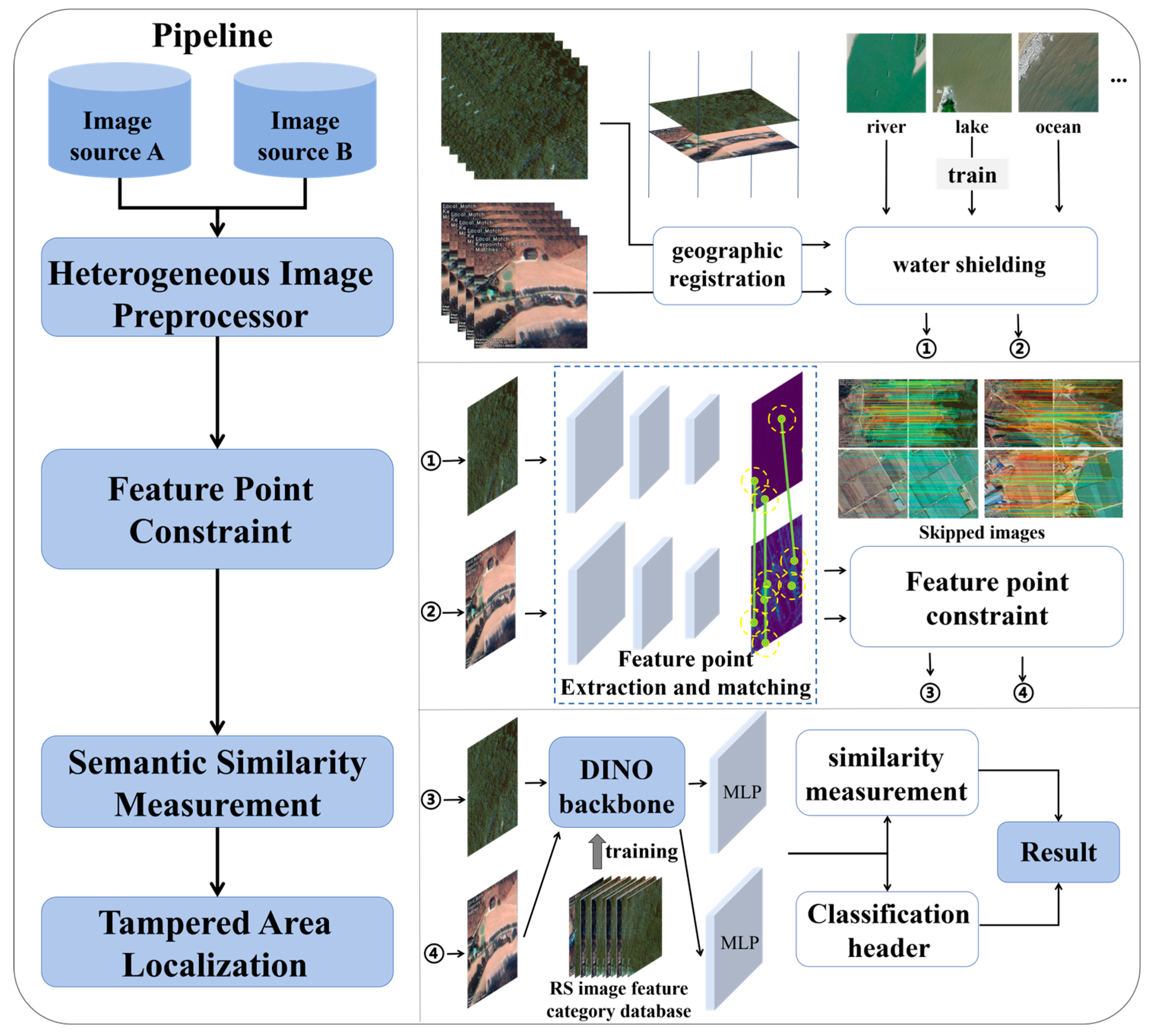
Here, we construct a high-precision heterogeneous satellite image manipulation localization (HSIML) framework to achieve our proposal. It aims to solve the potential image manipulation in remote sensing optical images. It conducts detection at the patch level, and can be divided into three parts:
(1) Heterogeneous Image Preprocessing Module: The projection coordinate systems and resolutions of heterogeneous images often exhibit differences, so these images need to be geographically aligned and subjected to some preprocessing operations, for example, water areas such as oceans and rivers will be treated as noise data and removed.
(2) Feature Point Constraint Module: Tampered images exhibit significant semantic differences, allowing the efficient determination of changes based on the quantity of feature points. Moreover, feature points offer high stability, enabling them to effectively mitigate variations in lighting, seasonal effects, and color channel disparities. This module extracts and matches feature points from the images, applying filtering rules to conduct an initial screening to identify candidate tampered patches.
(3) Semantic Similarity Measurement Module: The previous module differentiated based on the number of feature points and matched feature point groups. However, when the number of matched feature points is moderate and the quantity of feature points is also moderate, it is difficult to determine the confidence level when using the threshold method for judgment. At this point, we believe that determining whether the content of the two images is consistent still needs to return to the semantic information of the ground objects themselves. But at this stage, we do not need to identify what type of ground object it is. We only need to judge whether they are consistent by the similarity of the semantic features of the ground objects. Therefore, this module uses DINOv2 as the feature extraction backbone network and designs a classification network based on the saliency of features in remote sensing images. The module first performs feature classification and similarity measurements on the input images. Subsequently, based on predefined classification rules, it integrates the determined slice categories and image pair similarities to identify tampered regions. In addition, we also create a tampering detection dataset to alleviate the current scarcity of RS image datasets.
The remainder of this manuscript is organized as follows: Section 2 introduces tampering detection methods in remote sensing imagery. Section 3 describes the workflow and principles of the proposed method. Section 4 presents the study area and the tampering detection dataset proposed in this study, accompanied by a comprehensive experimental analysis and discussion of the proposed method. Section 5 gives our conclusion.

2. Related Works

2.1. IML on Satellite Images

Existing research on IML in RS images primarily focuses on detecting splicing and inpainting. There is relatively more research on splicing detection; for example, Horváth et al. [14] utilized deep belief networks, using patches as input units to learn the probability distribution of samples based on custom splicing tampering samples, subsequently generating heatmaps for the tampered regions. They also investigated the feasibility of Vision Transformers (ViTs) in image tampering, constructing a combined model for image classification that utilizes ViTs and morphological filters for post-processing to detect spliced tampered images [15]. The U-Net architecture is used to leverage the advantages of different semi-supervised splicing detection methods, incorporating nested attention mechanisms and Transformers to achieve optimal accuracy [16,17].
The research on inpainting detection in RS images is notably scarce. Adding semi-fragile watermarks before the publication of RS imagery and utilizing these watermarks as fingerprint verification [18] was a primary method employed to resist malicious image tampering in earlier practices. However, the widespread availability of RS images currently reduces the cost-effectiveness and applicability of watermarking. Deep learning methods such as generative adversarial networks (GANs) can be employed to learn feature distributions and representations within RS images [19], but the model’s effectiveness is constrained by insufficient training samples.
Additionally, there is a relative lack of methods in RS-IML that can be applied to multiple types of tampering detection. Meanwhile, the scarcity of datasets is a crucial factor restricting research in RS-IML. Directly learning the land cover distribution in RS images relies on original data, and the diversity of current image sources, along with the complexity of RS features, leads to insufficient robustness and transferability. Although Horváth et al. [20] applied anomaly detection methods to IML by training a single classifier to identify compression artifacts and information loss from splicing operations, they were still learning the original data’s distribution. In subsequent research, scholars shifted to using GANs to generate splicing tampered data and trained and tested based on this generated data; however, these datasets and methods have not been made open-source, making reproduction and further exploration of this research challenging.

2.2. Heterogeneous Satellite Image Manipulation Localization

To successfully perform the IML task in heterogeneous satellite images, the first step is to complete image co-registration [21,22] to ensure that pixels in the image pairs represent the same objects at corresponding locations. Subsequently, pixel-wise comparisons are performed to distinguish change areas. Relevant research on heterogeneous satellite image manipulation localization has not been found yet. But the principle and process of heterogeneous RSIML are quite analogous to change detection. So, we investigated the state-of-the-art methods for change detection.
Based on the change detection technology of deep learning, by continuously optimizing the network structure and loss function [23,24,25], and introducing the attention mechanism to enhance the ability of feature extraction [26], explore the multi-scale and multi temporal data fusion technology [27,28], so as to improve the ability of the model to capture subtle changes and the recognition accuracy of change areas in complex scenes. Although the change detection model based on deep learning has made significant progress, the accuracy decline is still the main problem in the following cases. Different sensors and imaging conditions may lead to significant differences between heterogeneous images, which may affect the performance of the model. The change detection algorithm needs to be able to accurately identify the changes in the main ground object targets, and is not affected by clouds, lighting angles, shadows and other unrelated factors. The current algorithm still has limitations in this regard. As an advanced technology, object-level change detection focuses on identifying the changes in specific objects in the image, which requires the model to have a higher semantic understanding and feature extraction ability, which is still a challenge.
Therefore, it can be predicted that change detection methods will encounter the problems of low accuracy and poor generalization when they are directly applied to large-scale IML tasks. It is still necessary to improve the methods’ robustness and accuracy: improve the robustness of the algorithm for different data acquisition parameters and environmental conditions (cloud, fog, illumination changes, etc.), and improve the accuracy of object-level semantic understanding, not just pixel-level feature understanding.

2.3. Image Consistency Measurement and Evaluation

Representative feature methods for evaluating image consistency have made significant progress in recent years, especially with the promotion of deep learning technology. Traditional feature extraction methods, such as sift, surf and orb, are popular because of their invariance to scale and rotation. The Scale-Invariant Feature Transform (SIFT) [29] algorithm extracts invariant image features to image scaling and rotation, thus mitigating the geometric and radiometric distortions caused by differences in lighting conditions and imaging angles from heterogeneous sensors. Dellinger et al. [30] used a comparison method to match key SIFT points to identify change areas. Building upon this, Wang et al. [31] combined SIFT with the ability to detect speckle-like structures in images, segmented around extracted key points to narrow down the detection scope, and further compared the two segmentation results to generate a change detection map. However, these methods still have limitations in dealing with challenging visual changes. Due to the complexity of features in RS images, traditional feature point detection algorithms, such as SIFT, often yield a significant number of redundant or insignificant features.
With the development of deep learning, feature extraction methods based on convolutional neural networks (CNNs), the transformer architecture, and the attention mechanism have become a research hotspot. These methods can automatically learn the hierarchical features of images and capture complex visual patterns from a low level to a high level. The extracted deep features have been proved to be very effective in the task of image consistency evaluation. For example, via an a contrario approach, the authors of [32] used a SIFT-like procedure to extract and characterize local keypoints and apply it to change detection tasks. SuperPoint [33] computes pixel-level feature point location through a fully-convolutional model to improve its cross-domain adaptation. Although feature-based methods are effective in urban scenes with clear geometric features in high-resolution remote sensing images, they may still fail in low-contrast and complex natural scenes [32,34]. In the latest research, researchers have begun to consider pixel-level change detection in urban building scenes, such as using a deep CNN [35], denoising diffusion probability model (DDPM) [36], Transformer [37], etc. However, the application scenarios of these studies are very focused and the image features are significant, which is different from our application scenario, so the effect of migration application is limited.

3. Methods

The proposed HSIML framework can be broadly divided into three parts: heterogeneous image preprocessing module, feature point constraint module, and feature classification and rule judgment module. The details of the model are illustrated in Figure 3 and will be discussed further in the following subsections.

3.1. Heterogeneous Image Preprocessor

The proposed method requires two sources of images for the IML process: a tampered image to be examined and a reference comparison image. However, these two types may differ regarding reference coordinate systems and image resolutions, necessitating rigorous geographic registration before proceeding with detection. Additionally, in practical applications, images covering natural water bodies such as oceans and lakes exhibit significant pseudo-changes, as the features between calm and turbulent water surfaces can vary markedly, leading to potential interference for the model.
To address these challenges, we designed a heterogeneous image preprocessor, which provides the detector and discriminator with high-quality data, enhancing feature-matching accuracy and ensuring the model fully utilizes its capabilities. It comprises two steps: geographic registration and water shielding.
For geographic registration, we first apply projection coordinate transformation to unify the coordinate systems and establish accurate spatial correspondences. Subsequently, we perform bilinear interpolation resampling on the harmonized images to obtain strictly registered images with consistent resolution.
For water shielding, we collect wave-like texture features of oceans, beaches, rivers, and lakes from RS images. A K-nearest neighbor classifier [38] is employed to train and shield these highly significant wave-like features during the image change detection process to reduce interference.

3.2. Feature Point Constraint Module

Due to the complexity of features in RS images, traditional feature point detection algorithms, such as SIFT, often yield a significant number of redundant or insignificant features. This study integrates the SuperPoint [33] algorithm to design a feature point constraint module to address this issue. First, feature points are extracted from heterogeneous RS images. Based on the extraction results, feature point matching is conducted, and erroneous match pairs are filtered using threshold constraints. The quantity of matched feature point pairs assesses the presence of tampering in the slices. For cases that cannot be distinguished, they are handled by the next module. The overall workflow of the module is illustrated in Figure 4.
The model takes heterogeneous images as input. The image encoder consists of three sets of convolutional layers, followed by max-pooling layers and ReLU activation functions. The descriptor for interest points draws from the UCN [39] model, initially outputting a semi-dense grid of descriptors, which are then processed using bicubic interpolation and normalized to unit length through L2 normalization to obtain the interest point descriptors. Subsequently, we employ brute-force matching to pair feature points from the heterogeneous images. Due to the inherent complexity of the images, there remains a substantial number of irrelevant points that require further elimination.
Consider two RS images A and B; the matching point pairs are composed of the x and y image coordinates from images A and B, and the distance r i :
M i = { x A i , y A i , x B i , y B i , r i }
M i is the successfully matched point pair i, x A i , y A i are the coordinates of the matched point pair in image A, x B i , y B i are the coordinates of the matched point pair in image B, x A i and x B i are the height of the corresponding point, y A i and y B i are the width of the corresponding point, and r i is the distance of the matched point pair. The distance threshold r is introduced to filter the matching results further. Ideally, after registration, the pixel coordinates of matching point pairs in two registered images should be the same or fall within an acceptable buffer zone. Therefore, this study considers constructing a buffer zone with a r radius. When the pixel coordinates of the matching points fall within this buffer zone, the match can be regarded as correct.
r r i = ( x A i x B i ) 2 + ( y A i y B i ) 2
The matching results of feature point clusters can reflect the changes in prominent features in the image. As shown in the example diagram A in Figure 4, when the features of the objects in the image are prominent, there are more extracted feature points, and correspondingly, there are more successfully matched point pairs, so it can be determined that no tampering has occurred. Conversely, if a change occurs, there may be a significant difference in the number of corresponding feature points, resulting in fewer successfully matched point pairs, as shown in the example diagram B in Figure 4. Therefore, this study considers that the number of matched feature point pairs can be used to roughly determine whether changes have occurred in the image, thereby preliminarily screening areas where changes are more likely to have occurred.
For a given threshold m for the number of feature point pairs, when the number of successfully matched point pairs exceeds this threshold, it is considered that the two images have a high degree of matching, indicating no change in the area. However, when the number of successfully matched feature point pairs is less than the given threshold, this study considers the influence of the number of feature points extracted from each image on the matching results. Specifically, when the number of feature points extracted from both images is less than the threshold m, it indicates that the features of the objects in the patch are weak, resulting in fewer feature points, as shown in the example diagram C in Figure 4. It requires the use of the next module to make a judgment.

3.3. Semantic Similarity Measurement

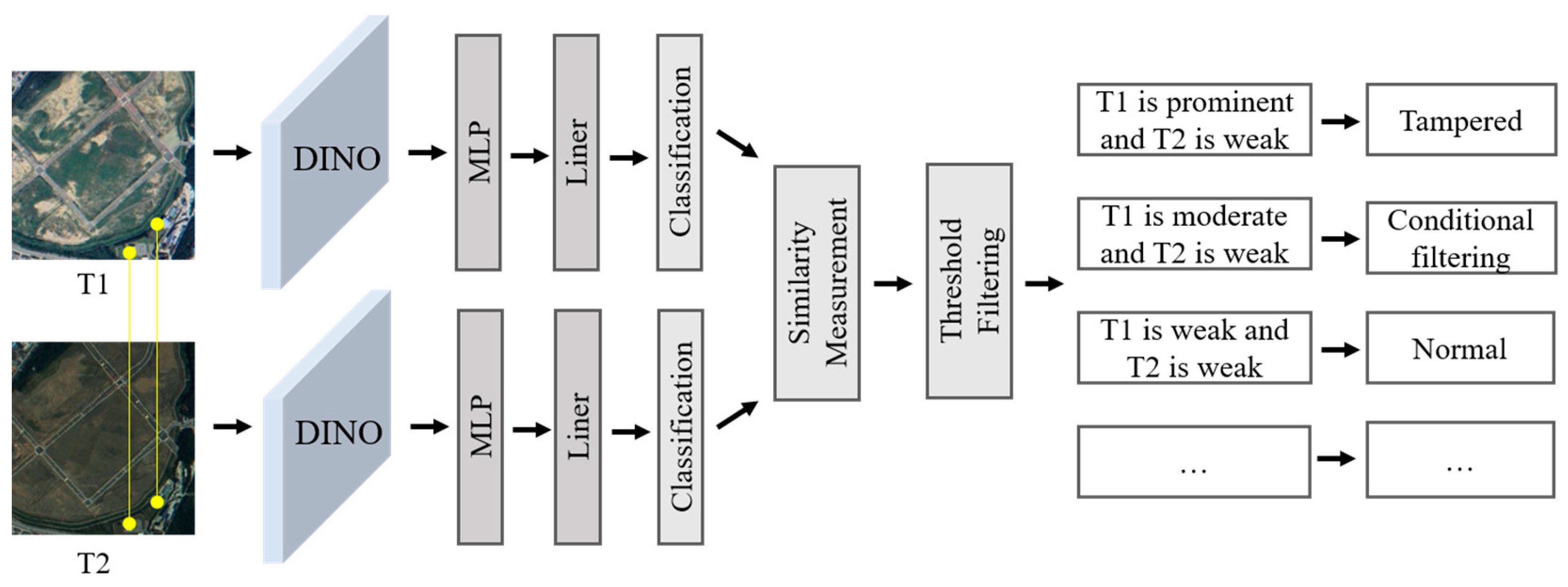
During large-scale image manipulation detection, there are often situations where the image features are not prominent, the feature points are sparse, or the matched feature point pairs do not satisfy threshold conditions from the previous module. As shown in Figure 5, there are few matched feature point pairs, so we propose assessing the spatial consistency of the images based on the semantic features of ground objects. We first use the fine-tuned DINOv2 model to extract the feature type labels of the images, respectively, and then calculate the cosine similarity between the image pairs. When the similarity meets the preset threshold, we consider the image pair to be matched successfully. If not, we then turn to using the extracted feature type labels to perform rule judgment and judge their consistency. The architecture of the semantic similarity measurement module is shown in Figure 5.
Specifically, this study initially gathers three typical land features—cities, forest and water bodies, and seasonal bare land—to construct a dataset of image feature categories. These categories correspond to three features: prominent, weak, and moderate as shown in Figure 6. Subsequently, we employ the DINOv2 [40] model as the backbone network for feature extraction, integrating a classic MLP for linear decoding. Training is conducted on the generated dataset to obtain a model suitable for feature classification.
The module utilizes heterogeneous RS images as input. It employs the trained DINO classification model to generate feature class labels for each image. For the two images, A and B, their features F A and F B ; and classification results A and B are obtained based on the module. The cosine similarity S i m of features is used to determine the similarity between the two patches:
S i m = F A · F B F A · F B
The similarity threshold s 1 is set for judgment. When the similarity S i m is larger than s 1 , it is considered that the images are similar, thus inferring that the patch has not changed. When the similarity is less than s 1 , the following rules are designed for further detection:
(1) When A is prominent and B is weak, or vice versa, indicating a substantial difference in feature prominence between A and B, it is inferred that the image has changed.
(2) When both A and B are either prominent or weak, suggesting that A and B are possibly located in areas characterized by prominent features such as urban landscapes or regions with weak features like forest or water bodies, it is inferred that the image has not changed.
(3) In the remaining cases, where at least one of the features is at a moderate level, the current threshold filtering criteria are too high in this condition, so a lower similarity threshold s 2 is set. If the similarity is larger than s 2 , it is considered that there is no change in the image; otherwise, the range of the patch is expanded by half and the entire model process is re-executed for detection. If the similarity is still lower than s 2 , it is determined that there is a change in the image.

4. Experiments

4.1. Dataset

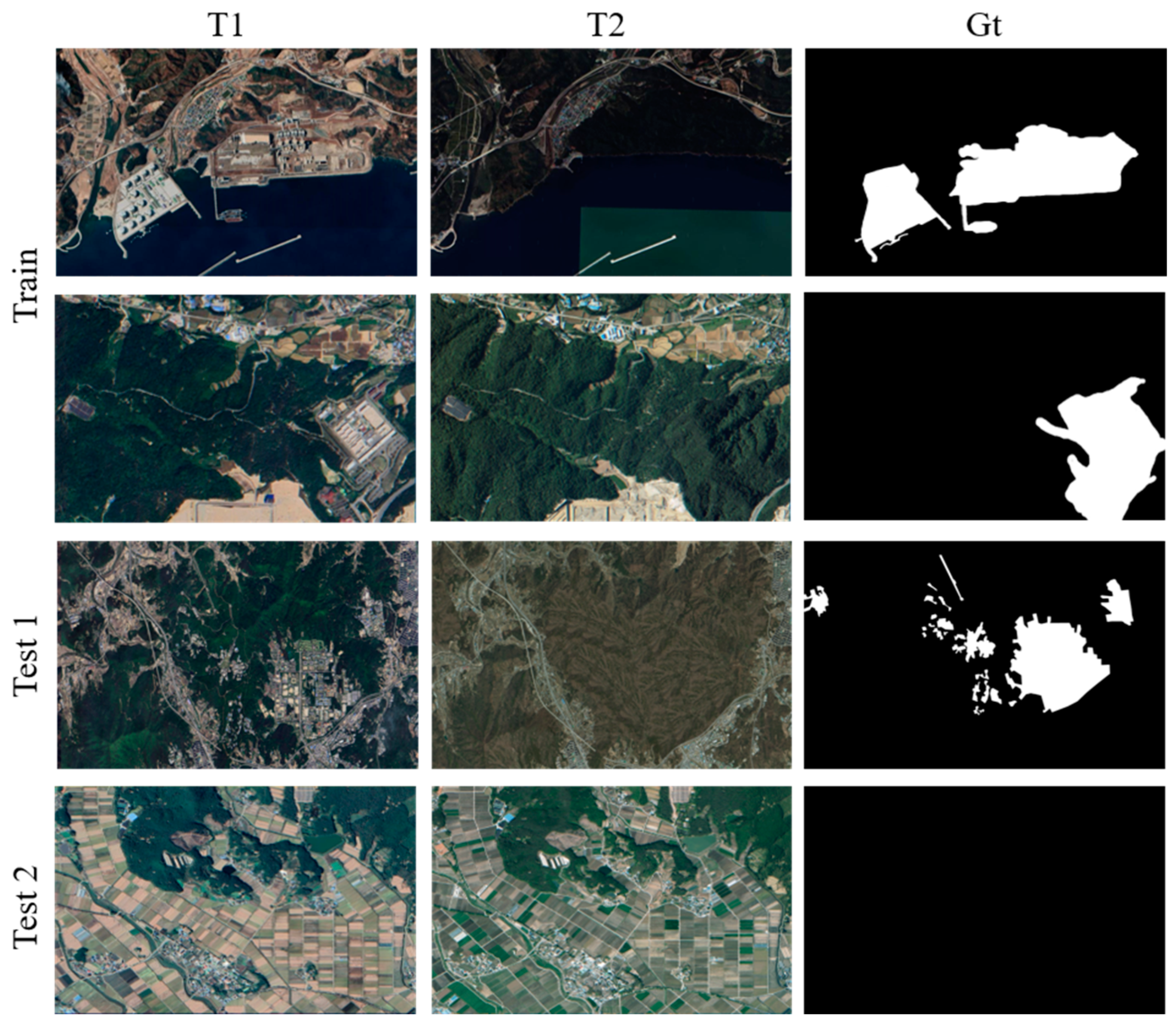
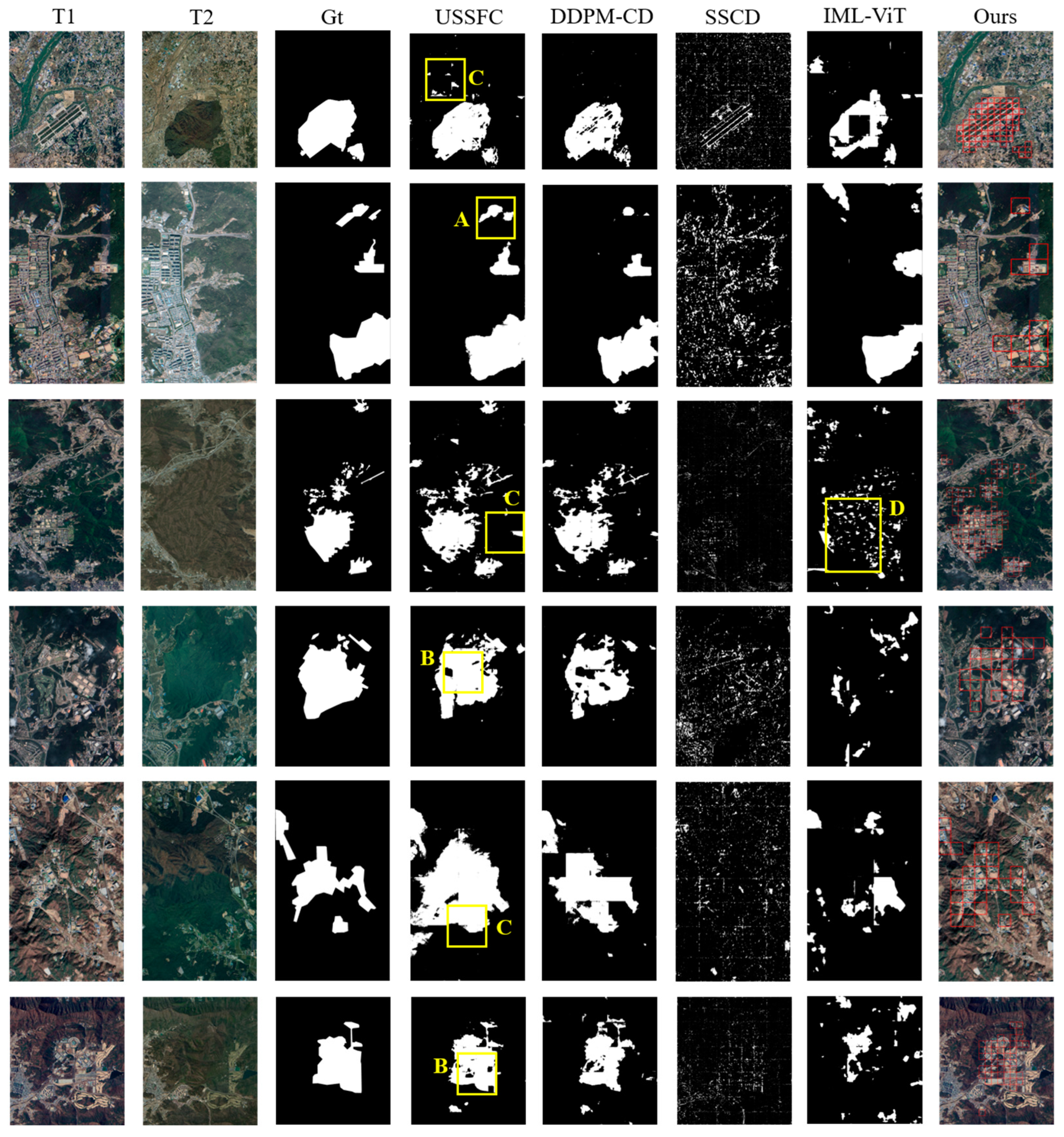
The dataset used in this study comes from a self-made dataset. It collects from two different map platforms with different map projection coordinate systems (WGS 84 and Pseudo Mercator), preprocessing work such as coordinate system unification and georeferencing is required. After that, we constructed a self-made dataset called the G-N Dataset (G-ND) for model training and testing through manual annotation. The dataset development is informed by the widely used DSIFN-CD [41] dataset in the field of change detection. The annotation process is facilitated using the LaMa [42] annotation tool IOPaint. The training set comprises 83 pairs of images, with image sizes ranging from 512*512 to 3700*3700. The images are cropped to 512*512 size, and 402 image pairs are obtained. Consistently with the DSIFN-CD dataset, data augmentation techniques including image rotation (45°, 90°, 135°, 180°, and 270°), flipping, noise addition, blur, and smoothing are applied and 4020 image pairs are obtained. Ninety percent of the data are randomly selected for training, and 10% for validation. The test set is divided into two parts: Test1, which was annotated and cropped in the same manner as the training set, yielding 338 image pairs, and Test2, introduced to evaluate the robustness of the model, with the dataset containing almost no tampered regions. We annotated and cropped the entire image and obtained 532 image pairs. The examples of training and test datasets are shown in Figure 7.

4.2. Ablation Experiment of Semantic Similarity Measurement Module

The evaluation indicators used in this study are F1 value and IoU. Our model is implemented based on PyTorch and trained on NVIDIA GeForce RTX 3090 GPU with 24GB memory for 100 epochs, with a batch size of 32. AdamW optimizer [43] with base learning is employed, and the cosine decay strategy is used with a learning rate ranging from 1 × 10 4 to 1 × 10 7 . Early stopping techniques are used during model training.
In Section 3.3, the proposed module utilizes DINOv2 as a backbone for image classification and feature extraction tasks. The performance of the DINO model directly determines the detection capability of the proposed model. Accordingly, based on the parameter settings of DINO, we tested the model’s performance under different conditions. The model backbone includes DINO with ViT, CiT [44], ResNet, and DINOv2 as shown in Table 1.
In Table 1, the DINO column has different model sizes, with S (small) and B (base) differing in network depth and parameter count. The values 8 and 16 refer to the patch sizes of ViT, where the minimum processing patches are 8 × 8 and 16 × 16. In the ViT-s/8 model, the accuracy is the lowest due to the small patch size: the training data have a resolution significantly lower than that of natural images, resulting in potential information loss from overly small patches, so the accuracy for patches of size 8 is inferior to that for size 16. Moreover, using ResNet as a backbone yields the worst performance, while other ViT-based backbone networks achieve relatively higher accuracy, which is attributed to the advantages of Transformers. The extensive use of convolutional layers risks losing critical information in high-level features, whereas the patching method employed by ViT preserves shallow features. In both DINO and DINOv2, small models often outperform base models, primarily due to the difference in task objectives. As our task aims to use feature classification to make judgments, though increasing model depth enhances feature extraction capability and improves detection accuracy, it also leads to an emphasis on finer details, which can amplify the contribution of weaker features, resulting in classification errors and decreased accuracy. Additionally, with relatively limited training data, deeper models are more prone to overfitting. The DINOv2-small model achieved the optimal F1 score, so this study utilizes DINOv2-small as the backbone network for the semantic similarity measurement module.

4.3. Comparative Analysis

The lack of research similar to this study makes direct comparative analysis challenging. To address this, we select recent state-of-the-art models from change detection to conduct tampering detection. To ensure a fair comparison, all the models are trained using the G-ND dataset. The test datasets use Test1 and Test2. The F1 score is utilized as the evaluation metric. Given the requirement for retraining, this study only considers open-source SOTA models, including the following:
USSFC [35] is an efficient ultra-lightweight spatial–spectral feature cooperation network based on deep CNNs, which combines a multi-scale decoupled convolution and the spatial–spectral feature cooperation (SSFC) strategy.
DDPM-CD [36] uses a pre-training denoising diffusion probabilistic model (DDPM) to learn the distribution of training data, and then employs it as a pre-trained feature extractor for change detection in downstream applications.
SSCD [37] is a novel summator–subtractor network for change detection, which calculates the initial channel changes through a summator and captures the initial spatial differences with a subtractor.
IML-ViT [10] is an image manipulation localization model based on the Vision Transformer (ViT). It addresses the weakness of a CNN in long-distance modeling capability and non-semantic modeling, constructing a ViT model with multi-scale feature extraction and edge-optimized monitoring capabilities.
Table 2 shows that in the Test1 dataset, the proposed model achieves the highest F1 score with 0.8657. In the Test2 dataset, the proposed model achieves the highest accuracy, recall, and F1 score results. This indicates that the proposed method not only exhibits high precision in locating tampered regions but also demonstrates sufficient generalization and robustness, effectively mitigating potential interference from various types of features in the images. Although the proposed method may not accurately delineate the contours of changed objects, it demonstrates the consistent detection of potential change regions. It offers higher robustness in practical applications within vast RS image datasets.

4.4. Visualization

To obtain a more intuitive understanding of our method’s functionality, we visualize the test results. Figure 8 shows the experiment on tampered region detection based on Test-1. It reveals that change detection methods can identify tampered regions but often suffer from incomplete localization (shown in area A), pixel loss (shown in area B), and false-positive detections (shown in area C). Similarly, the natural image tampering detection method also fails, especially when the tampered regions are excessively large or difficult to distinguish from their surrounding boundaries (shown in area D). In contrast, the red box area in the last column shows the detection result of our method, it reliably detects the position and extent of tampered regions.
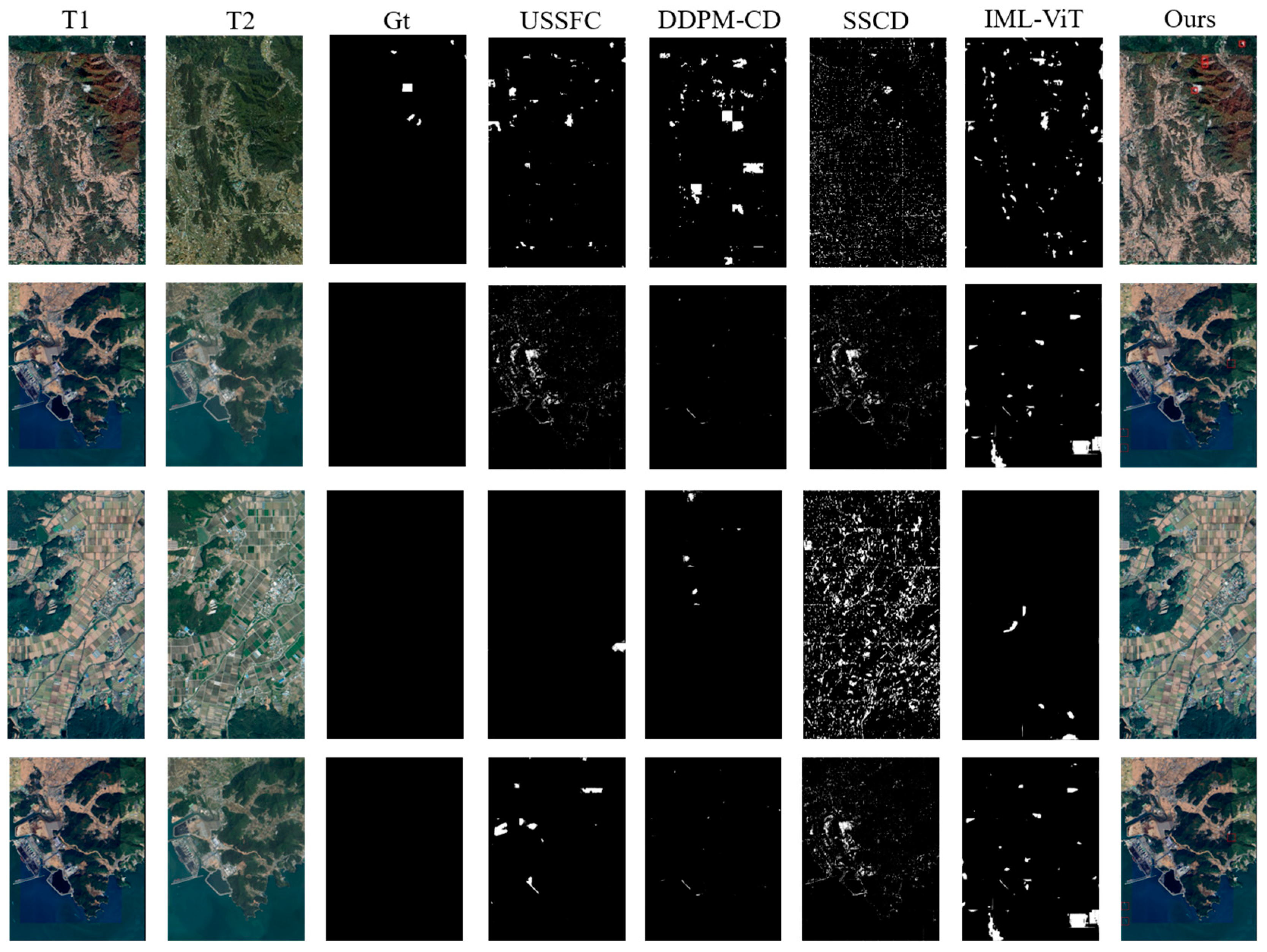
Figure 9 presents tampering detection experiments conducted on Test 2, which contains fewer tampered regions but exhibits greater natural variations in seasonality, lighting conditions, and other environmental factors. This dataset serves to validate the robustness of the model. From Figure 9, it can be observed that existing change detection models generate significantly more false positives, which is unacceptable for practical applications. In contrast, the red box area in the last column shows the detection result of our method, it demonstrates higher robustness in these challenging conditions.
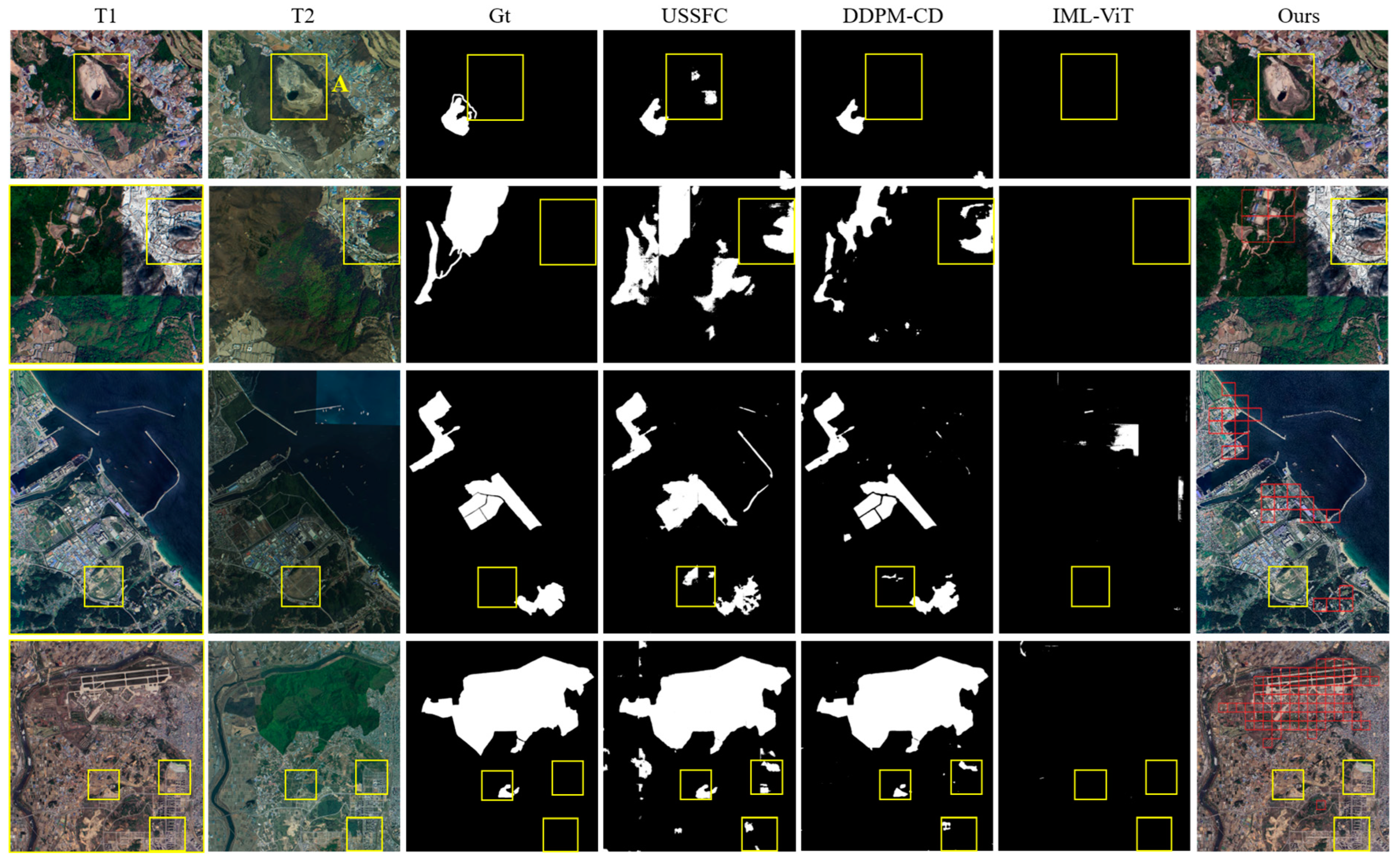
Figure 10 illustrates experiments conducted on changes induced by human activities. These images are selected from Test 1, and include not only tampered regions but also numerous regions of genuine change (highlighted in yellow boxes). It can be observed that change detection models often struggle to distinguish between real changes and tampered changes, thereby introducing varying degrees of additional pixels. The red box area in the last column shows the detection result of our method, it exhibits certain inhibitory effects on surface changes induced by human activities. Since genuine surface changes occur gradually, many strong invariant features remain preserved throughout the process. For instance, in the yellow region A, although certain areas within the region have experienced changes in their features, information such as roads and boundaries has remained unchanged. Despite occupying a relatively small pixel area, these significant invariant features contribute substantially to the feature point-based method proposed in this study, enabling the determination of a high degree of consistency between the two images rather than indicating substantially tampered alterations.
Based on the aforementioned results, our model demonstrates sufficient detection performance in IML tasks, robustness against variations due to lighting conditions, and capability to mitigate genuine changes stemming from potential human activities. This is attributed to our utilization of feature points to mitigate effects from illumination, seasonal changes, and color variations in images. When the semantic distribution and key features of images remain consistent, our method avoids introducing additional false positives. Furthermore, our feature-based classification method ensures precise localization of tampered regions.

4.5. Parameter Analysis

The parameters considered in this study mainly include the buffer radius r, the number of feature point pairs threshold m, and the similarity threshold s 1 and s 2 .
The first parameter, buffer radius r, represents the acceptable threshold for the coordinate distance between matched feature point pairs. After the strict registration of the images, the value of the buffer radius can be equivalent to the width of the image pixels. Therefore, the pixel value range of r is [0, 10], with a default value set to 5. Table 3 illustrates the relationship between the buffer radius and model accuracy. The smaller the r is, the more stringent the distance between matched points becomes, resulting in fewer matched pairs meeting the criteria. Consequently, fewer patches are deemed unchanged, leading to an increase in the number of patches requiring further detection to determine change. Therefore, as r increases, the precision rate gradually increases and the recall rate decreases. The F1 value is the largest when r = 3, so the buffer radius is set to 3.
The second parameter is the number of feature point pairs threshold m. The higher m value indicates a stricter exclusion criterion for areas where no change has occurred. In the application, since the patch size of this study is 128*128, in cases where features are not prominent, there might be relatively few matched point pairs. Therefore, considering the actual scenario, the default threshold value is set to 5. Table 4 illustrates the relationship between the threshold for the number of feature point pairs and model accuracy. As m increases, the criteria for identifying unchanged areas become more stringent. Consequently, the coarse screening process identifies more patches that could potentially change. Thus, the recall rate of the model gradually increases while the precision rate gradually decreases. The optimal F1 value is achieved when m is set to 5.
The third parameter is the similarity threshold s 1 and s 2 , which determines the similarity between patches of the same group. In this study, the change detection method employs a binary classification approach, where a higher similarity value indicates a higher likelihood that the slices in the group have not changed. Under normal circumstances, when the similarity is greater than 0.9, the images are essentially consistent. Therefore, the default similarity threshold of s 1 is set to 0.9, and the lower threshold s 2 is set to 0.85. To achieve a higher performance, we have conducted tests by lowering the similarity threshold to obtain more potential slices. Table 5 illustrates the relationship between the similarity threshold and the change in accuracy. Setting the similarity threshold too low may result in the missed detection of slices with subtle changes, leading to a loss in recall rate. As the similarity threshold increases, the instances where slices in the same group are determined to have not changed decrease, resulting in a gradual increase in the model’s recall rate. The highest F1 is achieved when the similarity threshold s 1 is set to 0.85. Accordingly, s 2 is set to a lower value of 0.8.

5. Discussion

The proposed HSIML has four hyperparameters that need to be determined, which would lead to complicated steps and additional workloads in actual applications or migration. This complexity not only increases the difficulty of debugging and optimization, but may also affect the performance and efficiency of the model. To simplify the computational and experimental workload arising from the numerous hyperparameters in practical applications, we have standardized the parameters by module and provided a method for quickly narrowing down the ranges. Specifically, the first two parameters pertain to the feature point constraint module. The buffer radius r ideally should correspond perfectly to matched point pairs, meaning r = 0. However, considering slight differences in feature point centers on the image, a default value of 3 is set, with a range of [1, 4] to be tested for the best precision. For the number of feature point pairs threshold m, the accuracy remains consistent when the number of matched pairs exceeds 5; thus, a default value of 5 is set, and adjustments are not recommended. The similarity threshold pertains to the semantic similarity measurement module. Based on parameter experimentation, it is advisable to maintain the default value of the similarity threshold s 1 at 0.85 and s 2 at 0.8. To achieve optimal accuracy, the parameter range of s 1 for testing can be set between [0.8, 0.9].
In the RSIML task, the model’s ability to resist interference is an important indicator of its robustness. Therefore, it is also crucial to assess whether the model’s accuracy can be maintained at a satisfactory level when the resolution of the tampered images is low or additional image compression is applied. To this end, we applied JPEG compression to the test samples at varying degrees to reduce their resolution and evaluated the model’s accuracy.
In Table 6, as the compression rate increases, although the model’s precision decreases, the overall F1 score remains relatively stable until the compression rate reaches 50%, after which there is a noticeable drop in accuracy. When the compression rate reaches 70%, the model’s accuracy has declined by 13%, but at this point, the differences between image pairs are eliminated and lose their reference significance. To this end, it can be concluded that the model maintains a certain robustness under low-resolution conditions.

6. Conclusions

Comparing heterogeneous satellite images enables the detection and localization of manipulation areas. The proposed HSIML framework achieves tampering detection in RS images by designing feature point rules and measuring semantic similarity. Significant semantic differences exist in tampered areas between heterogeneous images. Feature point matching and numerical constraints can locate tampered regions rapidly. The stability of feature points supports mitigating variations such as lighting and seasonal changes. Semantic similarity measurement is rooted in the semantic information of ground objects’ features. It utilizes semantic feature similarity to assess the consistency of image distribution. Its low complexity provides a foundation for achieving wide-ranging, high-precision tampering localization. Extensive empirical evidence has demonstrated the effectiveness of the proposed approach while maintaining sufficient generalizability. However, our method still has certain limitations, such as the inability to delineate the specific contours of tampered objects. Future research will focus on studying methods for the pixel-level localization of tampered areas in RS images.

Author Contributions

Conceptualization, W.G.; Data curation, C.S.; Formal analysis, C.S.; Methodology, Y.L.; Resources, W.G.; Software, Y.L.; Validation, R.W.; Visualization, C.S.; Writing—original draft, R.W.; Writing—review and editing, R.W. All authors have read and agreed to the published version of the manuscript.

Funding

This research was funded by National Natural Science Foundation of China, grant number 42071431.

Data Availability Statement

Data are contained within the article.

Conflicts of Interest

The authors declare no conflicts of interest.

References

  1. Liu, G.; Li, J.; Nie, P. Tracking the History of Urban Expansion in Guangzhou (China) during 1665–2017: Evidence from Historical Maps and Remote Sensing Images. Land Use Policy 2022, 112, 105773. [Google Scholar] [CrossRef]
  2. Basu, T.; Das, A.; Pereira, P. Exploring the Drivers of Urban Expansion in a Medium-Class Urban Agglomeration in India Using the Remote Sensing Techniques and Geographically Weighted Models. Geogr. Sustain. 2023, 4, 150–160. [Google Scholar] [CrossRef]
  3. Qiu, C.; Zhang, X.; Tong, X.; Guan, N.; Yi, X.; Yang, K.; Zhu, J.; Yu, A. Few-Shot Remote Sensing Image Scene Classification: Recent Advances, New Baselines, and Future Trends. ISPRS J. Photogramm. Remote Sens. 2024, 209, 368–382. [Google Scholar] [CrossRef]
  4. Li, X.; Wen, C.; Hu, Y.; Zhou, N. RS-CLIP: Zero Shot Remote Sensing Scene Classification via Contrastive Vision-Language Supervision. Int. J. Appl. Earth Obs. Geoinf. 2023, 124, 103497. [Google Scholar] [CrossRef]
  5. Wang, J.; Li, W.; Zhang, M.; Tao, R.; Chanussot, J. Remote-Sensing Scene Classification via Multistage Self-Guided Separation Network. IEEE Trans. Geosci. Remote Sens. 2023, 61, 5615312. [Google Scholar] [CrossRef]
  6. Lv, Z.; Liu, T.; Benediktsson, J.A.; Falco, N. Land Cover Change Detection Techniques: Very-High-Resolution Optical Images: A Review. IEEE Geosci. Remote Sens. Mag. 2022, 10, 44–63. [Google Scholar] [CrossRef]
  7. Das, S.; Angadi, D.P. Land Use Land Cover Change Detection and Monitoring of Urban Growth Using Remote Sensing and GIS Techniques: A Micro-Level Study. GeoJournal 2022, 87, 2101–2123. [Google Scholar] [CrossRef]
  8. Lv, Z.; Zhong, P.; Wang, W.; You, Z.; Benediktsson, J.A.; Shi, C. Novel Piecewise Distance Based on Adaptive Region Key-Points Extraction for LCCD With VHR Remote-Sensing Images. IEEE Trans. Geosci. Remote Sens. 2023, 61, 5607709. [Google Scholar] [CrossRef]
  9. Edwards, J. NGA’s Todd Myers: China Uses GAN Technique to Tamper With Earth Images 2019. Available online: https://executivegov.com/2019/04/ngas-todd-myers-china-uses-gan-technique-to-tamper-with-earth-images (accessed on 1 April 2019).
  10. Ma, X.; Du, B.; Jiang, Z.; Hammadi, A.Y.A.; Zhou, J. IML-ViT: Benchmarking Image Manipulation Localization by Vision Transformer. arXiv 2023, arXiv:2307.14863. [Google Scholar] [CrossRef]
  11. Horvath, J. Manipulation Detection and Localization for Satellite Imagery. Ph.D. Thesis, Purdue University Graduate School, West Lafayette, IN, USA, 2022. [Google Scholar]
  12. Bartusiak, E.R.; Yarlagadda, S.K.; Güera, D.; Bestagini, P.; Tubaro, S.; Zhu, F.M.; Delp, E.J. Splicing Detection and Localization in Satellite Imagery Using Conditional GANs. In Proceedings of the 2019 IEEE Conference on Multimedia Information Processing and Retrieval (MIPR), San Jose, CA, USA, 28–30 March 2019; pp. 91–96. [Google Scholar]
  13. Montserrat, D.M.; Horváth, J.; Yarlagadda, S.K.; Zhu, F.; Delp, E.J. Generative Autoregressive Ensembles for Satellite Imagery Manipulation Detection 2020. In Proceedings of the 12th IEEE International Workshop on Information Forensics and Security (WIFS), New York, NY, USA, 6–11 December 2020; pp. 1–6. [Google Scholar] [CrossRef]
  14. Horváth, J.; Montserrat, D.M.; Hao, H.; Delp, E.J. Manipulation Detection in Satellite Images Using Deep Belief Networks. In Proceedings of the 2020 IEEE/CVF Conference on Computer Vision and Pattern Recognition Workshops (CVPRW), Seattle, WA, USA, 14–19 June 2020; pp. 2832–2840. [Google Scholar]
  15. Horváth, J.; Baireddy, S.; Hao, H.; Montserrat, D.M.; Delp, E.J. Manipulation Detection in Satellite Images Using Vision Transformer. arXiv 2021, arXiv:2105.06373. [Google Scholar] [CrossRef]
  16. Horváth, J.; Montserrat, D.M.; Delp, E.J.; Horváth, J. Nested Attention U-Net: A Splicing Detection Method for Satellite Images. In Proceedings of the Pattern Recognition. ICPR International Workshops and Challenges; Del Bimbo, A., Cucchiara, R., Sclaroff, S., Farinella, G.M., Mei, T., Bertini, M., Escalante, H.J., Vezzani, R., Eds.; Springer International Publishing: Cham, Switzerland, 2021; pp. 516–529. [Google Scholar]
  17. Horváth, J.; Xiang, Z.; Cannas, E.D.; Bestagini, P.; Tubaro, S.; Iii, E.J.D. Sat U-Net: A Fusion Based Method for Forensic Splicing Localization in Satellite Images. In Proceedings Volume, Multimodal Image Exploitation and Learning 2022; SPIE: Bellingham, WA, USA, 2022; Volume 12100, p. 1210002. [Google Scholar]
  18. Ho, A.T.S.; Zhu, X.; Woon, W.M. A Semi-Fragile Pinned Sine Transform Watermarking System for Content Authentication of Satellite Images. In Proceedings of the 2005 IEEE International Geoscience and Remote Sensing Symposium, 2005—IGARSS ’05, Seoul, Republic of Korea, 29 July 2005; Volume 2, p. 4. [Google Scholar]
  19. Yarlagadda, S.K.; Güera, D.; Bestagini, P.; Zhu, F.M.; Tubaro, S.; Delp, E.J. Satellite Image Forgery Detection and Localization Using GAN and One-Class Classifier. arXiv 2018, arXiv:1802.04881. [Google Scholar] [CrossRef]
  20. Horvath, J.; Guera, D.; Kalyan Yarlagadda, S.; Bestagini, P.; Maggie Zhu, F.; Tubaro, S.; Delp, E.J. Anomaly-Based Manipulation Detection in Satellite Images. Networks 2019, 29, 62–71. [Google Scholar]
  21. Klaric, M.N.; Claywell, B.C.; Scott, G.J.; Hudson, N.J.; Sjahputera, O.; Li, Y.; Barratt, S.T.; Keller, J.M.; Davis, C.H. GeoCDX: An Automated Change Detection and Exploitation System for High-Resolution Satellite Imagery. IEEE Trans. Geosci. Remote Sens. 2013, 51, 2067–2086. [Google Scholar] [CrossRef]
  22. Han, Y.; Bovolo, F.; Bruzzone, L. An Approach to Fine Coregistration Between Very High Resolution Multispectral Images Based on Registration Noise Distribution. IEEE Trans. Geosci. Remote Sens. 2015, 53, 6650–6662. [Google Scholar] [CrossRef]
  23. Bergamasco, L.; Saha, S.; Bovolo, F.; Bruzzone, L. Unsupervised Change Detection Using Convolutional-Autoencoder Multiresolution Features. IEEE Trans. Geosci. Remote Sens. 2022, 60, 4408119. [Google Scholar] [CrossRef]
  24. Yang, B.; Qin, L.; Liu, J.; Liu, X. UTRNet: An Unsupervised Time-Distance-Guided Convolutional Recurrent Network for Change Detection in Irregularly Collected Images. IEEE Trans. Geosci. Remote Sens. 2022, 60, 4410516. [Google Scholar] [CrossRef]
  25. Feng, Y.; Jiang, J.; Xu, H.; Zheng, J. Change Detection on Remote Sensing Images Using Dual-Branch Multilevel Intertemporal Network. IEEE Trans. Geosci. Remote Sens. 2023, 61, 4401015. [Google Scholar] [CrossRef]
  26. Zhang, M.; Liu, Z.; Feng, J.; Liu, L.; Jiao, L. Remote Sensing Image Change Detection Based on Deep Multi-Scale Multi-Attention Siamese Transformer Network. Remote Sens. 2023, 15, 842. [Google Scholar] [CrossRef]
  27. Hao, M.; Yang, C.; Lin, H.; Zou, L.; Liu, S.; Zhang, H. Bi-Temporal Change Detection of High-Resolution Images by Referencing Time Series Medium-Resolution Images. Int. J. Remote Sens. 2023, 44, 3333–3357. [Google Scholar] [CrossRef]
  28. Han, C.; Wu, C.; Guo, H.; Hu, M.; Chen, H. HANet: A Hierarchical Attention Network for Change Detection with Bitemporal Very-High-Resolution Remote Sensing Images. IEEE J. Sel. Top. Appl. Earth Obs. Remote Sens. 2023, 16, 3867–3878. [Google Scholar] [CrossRef]
  29. Lowe, D.G. Distinctive Image Features from Scale-Invariant Keypoints. Int. J. Comput. Vis. 2004, 60, 91–110. [Google Scholar] [CrossRef]
  30. Dellinger, F.; Delon, J.; Gousseau, Y.; Michel, J.; Tupin, F. Change Detection for High Resolution Satellite Images, Based on SIFT Descriptors and an a Contrario Approach. In Proceedings of the 2014 IEEE Geoscience and Remote Sensing Symposium, Quebec City, QC, Canada, 13–18 July 2014; pp. 1281–1284. [Google Scholar]
  31. Wang, Y.; Du, L.; Dai, H. Unsupervised SAR Image Change Detection Based on SIFT Keypoints and Region Information. IEEE Geosci. Remote Sens. Lett. 2016, 13, 931–935. [Google Scholar] [CrossRef]
  32. Liu, G.; Gousseau, Y.; Tupin, F. A Contrario Comparison of Local Descriptors for Change Detection in Very High Spatial Resolution Satellite Images of Urban Areas. IEEE Trans. Geosci. Remote Sens. 2019, 57, 3904–3918. [Google Scholar] [CrossRef]
  33. DeTone, D.; Malisiewicz, T.; Rabinovich, A. SuperPoint: Self-Supervised Interest Point Detection and Description. In Proceedings of the 2018 IEEE Conference on Computer Vision and Pattern Recognition Workshops, Salt Lake City, UT, USA, 18–22 June 2018. [Google Scholar]
  34. Cui, H.; Shen, S.; Gao, W.; Liu, H.; Wang, Z. Efficient and Robust Large-Scale Structure-from-Motion via Track Selection and Camera Prioritization. ISPRS J. Photogramm. Remote Sens. 2019, 156, 202–214. [Google Scholar] [CrossRef]
  35. Lei, T.; Geng, X.; Ning, H.; Lv, Z.; Gong, M.; Jin, Y.; Nandi, A.K. Ultralightweight Spatial–Spectral Feature Cooperation Network for Change Detection in Remote Sensing Images. IEEE Trans. Geosci. Remote Sens. 2023, 61, 4402114. [Google Scholar] [CrossRef]
  36. Bandara, W.G.C.; Nair, N.G.; Patel, V.M. DDPM-CD: Denoising Diffusion Probabilistic Models as Feature Extractors for Change Detection. arXiv 2024, arXiv:2206.11892. [Google Scholar] [CrossRef]
  37. Wang, L.; Fang, Y.; Li, Z.; Wu, C.; Xu, M.; Shao, M. Summator–Subtractor Network: Modeling Spatial and Channel Differences for Change Detection. IEEE Trans. Geosci. Remote Sens. 2024, 62, 5604212. [Google Scholar] [CrossRef]
  38. Touazi, A.; Bouchaffra, D. A K-Nearest Neighbor Approach to Improve Change Detection from Remote Sensing: Application to Optical Aerial Images. In Proceedings of the 2015 15th International Conference on Intelligent Systems Design and Applications (ISDA), Marrakesh, Morocco, 14–16 December 2015; pp. 98–103. [Google Scholar]
  39. Choy, C.B.; Gwak, J.; Savarese, S.; Chandraker, M. Universal Correspondence Network. In Proceedings of the Advances in Neural Information Processing Systems; Curran Associates, Inc.: New York, NY, USA, 2016; Volume 29. [Google Scholar]
  40. Oquab, M.; Darcet, T.; Moutakanni, T.; Vo, H.; Szafraniec, M.; Khalidov, V.; Fernandez, P.; Haziza, D.; Massa, F.; El-Nouby, A.; et al. DINOv2: Learning Robust Visual Features without Supervision. arXiv 2023, arXiv:2304.07193. [Google Scholar] [CrossRef]
  41. Zhang, C.; Yue, P.; Tapete, D.; Jiang, L.; Shangguan, B.; Huang, L.; Liu, G. A Deeply Supervised Image Fusion Network for Change Detection in High Resolution Bi-Temporal Remote Sensing Images. ISPRS J. Photogramm. Remote Sens. 2020, 166, 183–200. [Google Scholar] [CrossRef]
  42. Suvorov, R.; Logacheva, E.; Mashikhin, A.; Remizova, A.; Ashukha, A.; Silvestrov, A.; Kong, N.; Goka, H.; Park, K.; Lempitsky, V. Resolution-Robust Large Mask Inpainting with Fourier Convolutions. In Proceedings of the IEEE/CVF Winter Conference on Applications of Computer Vision, Virtual, 5–9 January 2021. [Google Scholar]
  43. Loshchilov, I.; Hutter, F. Decoupled Weight Decay Regularization. arXiv 2019, arXiv:1711.05101. [Google Scholar] [CrossRef]
  44. El-Nouby, A.; Touvron, H.; Caron, M.; Bojanowski, P.; Douze, M.; Joulin, A.; Laptev, I.; Neverova, N.; Synnaeve, G.; Verbeek, J.; et al. XCiT: Cross-Covariance Image Transformers. arXiv 2021, arXiv:2106.09681. [Google Scholar] [CrossRef]
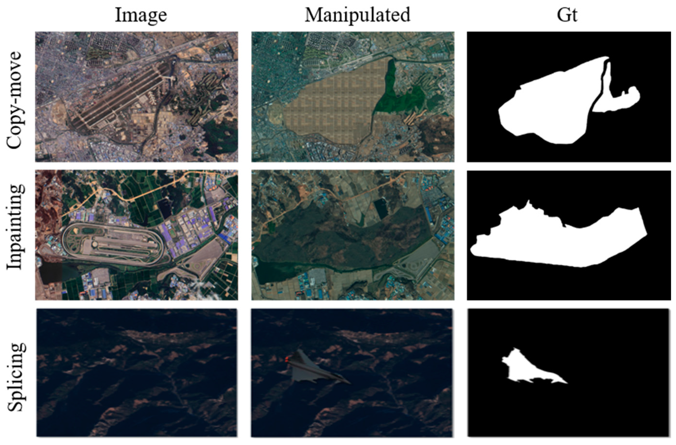
Figure 1. Three types of tampering methods in remote sensing images. Copy-move involves tampering by copying existing elements within the image. Inpainting refers to tampering by erasing objects in the image. Splicing is achieved by stitching elements from other images into a different image for tampering.
Remotesensing 16 03719 g001
Figure 2. Three types of inconsistencies between multiple remote sensing images.
Remotesensing 16 03719 g002
Figure 3. The illustration of the proposed heterogeneous satellite image manipulation localization framework (HSIML).
Remotesensing 16 03719 g003
Figure 4. The architecture of the feature point constraint module. It accepts heterogeneous RS images as input. After processing through feature point extraction, matching, filtering, and rule-based constraints, the module yields results indicating potential tampering in the patches.
Remotesensing 16 03719 g004
Figure 5. The architecture of semantic similarity measurement module. It takes heterogeneous RS images as input, utilizing the fine-tuned DIONv2 model to generate feature class labels and compute image similarity. Based on a predefined threshold and established rules, the module finally detects potentially manipulated patches.
Remotesensing 16 03719 g005
Figure 6. Three types of feature class labels.
Remotesensing 16 03719 g006
Figure 7. Examples of our self-made G-N dataset. T1 and T2 are from different sources, Gt is the manually annotated ground truth, Predict is the detection result using the proposed model. Zoom in to see clearer details.
Remotesensing 16 03719 g007
Figure 8. The visualization results of the models on Test 1. Zoom in to see clearer details.
Remotesensing 16 03719 g008
Figure 9. The visualization results of the models on Test 2. Zoom in to see clearer details.
Remotesensing 16 03719 g009
Figure 10. The visualization results of the models on surface changes induced by human activities. The yellow box indicates surface changes resulting from expansion or cultivation. Zoom in to see clearer details.
Remotesensing 16 03719 g010
Table 1. Evaluation results with different model backbones.
ModelPrecision (%)Recall (%)F1 (%)IoU (%)
xcit_small82.0386.9884.4373.05
resnet5087.3767.0775.8961.14
DINOVit-S/1680.9075.7278.2264.24
Vit-S/878.6863.0970.0253.88
Vit-B/1679.5174.1876.7562.28
Vit-B/874.0670.3772.1756.46
DINOv2Dinov2-small91.4582.1886.5776.32
Dinov2-base87.7883.7485.7175.00
Table 2. Evaluation results with other models on two test sets.
DatasetsMethodsPrecision (%)Recall (%)F1 (%)
Test1USSFC64.9595.3177.25
DDPM-CD73.3189.2180.48
SSCD21.0693.5834.38
IML-ViT57.3548.1252.33
Ours91.4582.1886.57
Test2USSFC98.9286.9992.57
DDPM-CD98.6189.4293.79
SSCD98.9331.0947.31
IML-ViT98.0381.0388.72
Ours98.9491.5795.11
Table 3. The relationship between buffer radius r and accuracy.
rPrecision (%)Recall (%)F1 (%)
180.1884.9282.48
280.9683.9782.44
382.0483.4482.73
482.4779.1480.77
582.8878.3080.52
683.2177.3780.18
783.2976.6779.84
Table 4. The relationship between the threshold of feature point pairs m and accuracy.
mPrecision (%) ↑Recall (%) ↑F1 (%) ↑
183.1270.4976.29
282.6078.1180.29
382.1779.8881.01
482.0480.4381.23
581.9980.5881.28
681.9680.6281.28
781.9680.6281.28
Table 5. The relationship between similarity threshold and accuracy.
s 1 s 2 Precision (%)Recall (%)F1 (%)
0.600.5593.3322.7736.61
0.650.6094.5642.8058.93
0.700.6593.0558.5071.84
0.750.7089.4169.8478.42
0.800.7584.5777.4680.86
0.850.8081.9680.6281.28
0.900.8580.0281.6980.85
Table 6. The relationship between compression rate and accuracy.
Compression Rate (%)Precision (%)Recall (%)F1 (%)
091.4582.1886.57
1090.6881.6385.92
2089.8482.4385.98
3087.9383.0085.39
4086.4283.2484.80
5081.9382.5582.24
6078.3582.0980.18
7068.3079.8273.61
8063.8780.4971.22
Disclaimer/Publisher’s Note: The statements, opinions and data contained in all publications are solely those of the individual author(s) and contributor(s) and not of MDPI and/or the editor(s). MDPI and/or the editor(s) disclaim responsibility for any injury to people or property resulting from any ideas, methods, instructions or products referred to in the content.