A Multi-Scale Feature Fusion Based Lightweight Vehicle Target Detection Network on Aerial Optical Images

Abstract

Vehicle detection with optical remote sensing images has become widely applied in recent years. However, the following challenges have remained unsolved during remote sensing vehicle target detection. These challenges include the dense and arbitrary angles at which vehicles are distributed and which make it difficult to detect them; the extensive model parameter (Param) that blocks real-time detection; the large differences between larger vehicles in terms of their features, which lead to a reduced detection precision; and the way in which the distribution in vehicle datasets is unbalanced and thus not conducive to training. First, this paper constructs a small dataset of vehicles, MiVehicle. This dataset includes 3000 corresponding infrared and visible image pairs, offering a more balanced distribution. In the infrared part of the dataset, the proportions of different vehicle types are as follows: cars, 48%; buses, 19%; trucks, 15%; freight, cars 10%; and vans, 8%. Second, we choose the rotated box mechanism for detection with the model and we build a new vehicle detector, ML-Det, with a novel multi-scale feature fusion triple cross-criss FPN (TCFPN), which can effectively capture the vehicle features in three different positions with an mAP improvement of 1.97%. Moreover, we propose LKC–INVO, which allows involution to couple the structure of multiple large kernel convolutions, resulting in an mAP increase of 2.86%. We also introduce a novel C2F_ContextGuided module with global context perception, which enhances the perception ability of the model in the global scope and minimizes model Params. Eventually, we propose an assemble–disperse attention module to aggregate local features so as to improve the performance. Overall, ML-Det achieved a 3.22% improvement in accuracy while keeping Params almost unchanged. In the self-built small MiVehicle dataset, we achieved 70.44% on visible images and 79.12% on infrared images with 20.1 GFLOPS, 78.8 FPS, and 7.91 M. Additionally, we trained and tested our model on the following public datasets: UAS-AOD and DOTA. ML-Det was found to be ahead of many other advanced target detection algorithms.

1. Introduction

Remote sensing technology applies various sensing instruments to collect, process, and analyze electromagnetic wave information that is radiated and reflected by remote targets, and to perceive the relative positions of objects on the ground in order to obtain extensive information on ground objects [1]. With the rapid development of aviation aerospace technologies, such as drones and satellites, the resolution of optical remote sensing images has been gradually improved, which provides strong technical support for various visual tasks, including target identification. Vehicles are an indispensable part of transportation. Many algorithms have been developed based on enhancements to YOLO. Yin et al. [2] created YOLOv4_CPSBi, which improves the detection of land targets that are small and densely distributed. Zhang et al. [3] proposed a YOLO detector that incorporates a novel flip mosaic method, specifically designed to address vehicle targets that are prone to occlusion. Carrasco et al. [4] employed a multi-scale mechanism along with channel and spatial attention mechanisms to improve the precision of the original YOLOv5 from 63.87% to 96.34%, with only a 1.53 M increase in Param. By providing accurate and timely detection of vehicles through remote sensing, it is possible to access real-time transportation conditions, reduce congestion, and lower the rate of traffic accidents. In general, the larger the model’s Param, the greater its ability to express features. However, storing too many Params can lead to a bloated model and result in poor detection. In actual deployment, due to the limited storage resources of remote sensing equipment, it is necessary for the model to become lightweight while maintaining its precision. This is in order for it to be able to utilize the storage resources more reasonably and efficiently. The following challenges arise during the vehicle detection process for optical remote sensing images:

• Vehicle targets exhibit a dense, multi-angle distribution: Remote sensing images of vehicles present arbitrary angles, and their dense distribution often leads to overlapping bounding boxes, using horizontal box methods for vehicle detection.
• A large number of model Params will impair real-time detection: It has become routine to enhance the width and depth of a network to improve its precision; however, this also results in a higher number of Params, consumes greater computational resources and is not conducive to practical deployment.
• Large vehicles with diverse features and low detection accuracy: The actual remote sensing capture process requires the imaging of a large range of scenes, with large variations in the angle of capture and imaging height. Large vehicles are less common, making it challenging to identify general features by which to distinguish them.
• Significant imbalance in the distribution of vehicle types and numbers: In the vehicle dataset, small private cars are numerous, making up the majority. Large vehicles are fewer in number, leading to an unbalanced distribution of different vehicle types and resulting in lower accuracy and significant overfitting.

With the advancement of deep learning, numerous outstanding rotating box-based target detection algorithms have emerged. As shown in Figure 1, when the target presents a dense, multi-angle distribution, using a horizontal frame to select the vehicle target is likely to cause overlap between boxes, which can interfere with visual judgment. There have been many public datasets using rotating box annotation in the field of remote sensing detection, such as DOTA [5], DIOR-R [6], DroneVehicle [7], and UCAS-AOD [8]. Rotating box-based target detection can be divided into two-stage, one-stage, and anchor-free box target detection algorithms according to the mechanism. The anchor-free box detection method does not need to set the anchor box Params but does have a lower precision. In general, two-stage rotary detectors have the highest accuracy, but have a relatively slow inference speed. Instead of generating candidate boxes, one-stage detection algorithms accomplish the detection task in a single forward propagation process using a dense grid or anchor box, and are typically faster than two-stage algorithms.

The low precision in large vehicle detection is due to feature differences and inadequate extraction, and numerous neck structures are now available to enhance the feature extraction capability of the model. The FPN structure [9] forms a top-down path by upsampling the convolutional layers extracted from the backbone, and then fuses the deeper high-level features with the shallower low-level features using lateral connections. PAFPN structure [10] adds a bottom-up path to FPN, augmenting the entire feature pyramid with precise localization signals from the lower layers, shortening the information path from the bottom to the top. The NASFPN structure [11] uses a “network search space” approach, searching the topology of a regular feature network and then reuses the same sub-modules. The BiFPN structure [12] configures different feature weights for different input features, while using a two-way cross-scale connectivity approach that combines iterative top-down and bottom-up methods to fuse multi-scale features and reduce feature loss. The HSFPN structure [13] employs channel attention (CA) [14] and a dimension matching (DM) mechanism to filter the feature maps at various scales and obtain information from different channels. The selective feature fusion (SFF) module can then effectively enhance the detection of multi-scale objects.

Model complexity and computational volume have hindered the deployment of vision algorithms on mobile platforms, so a large number of lightweight network structures have been proposed to compress the model size. SqueezeNet [15] reduces model Params by reducing the number of input channels for the 3 × 3 convolution and replacing the 3 × 3 convolution with a large number of 1 × 1 convolutions. MobileNet series models were originally designed to address the challenges of deploying large models on mobile embedded devices. MobileNet v1 [16] is a lightweight network built with depth-wise separable convolution, and its lightweight nature is related to the size of convolutional kernel. MobileNet v2 [17] proposes an inverted residual bottleneck module, which uses a 1 × 1 increase in convolutional dimension to reduce the loss of information, and then reduces the dimension back to the original number of channels after the separation of convolutions for the operation. This makes the model lightweight while improving its performance. MobileNet v3 [18] adopts a network structure search technique and uses the NetAdapt algorithm to finetune the network layers under limited resources. ShuffleNetv1 [19] combines point-by-point grouped convolution to reduce model Params, and the channel shuffle method to increase the correlation between different groups to prevent information loss. ShuffleNetv2 [20] uses a channel split operation, which reduces the fragmentation of the network and improves the speed of the model. EfficientNet [21] uses an NAS search technique, which uniformly scales input resolution, network depth, and network width to provide better feature representation compared with CNN networks. GhostNet [22] first compresses the input image with the number of channels, then obtains more feature maps with DSConv, finally obtaining the result by concat. RepVGG [23] uses a reparameterization technique to decouple the multi-branch model into an inference smoothing model, which saves memory and improves the inference speed.

The main work accomplished In this paper Ih Is different from past methods Is as follows:

• The development of a new neck structure, TCFPN, which allows the ML-Det network to efficiently fuse three feature maps of different scales, thereby extracting more vehicle target features and improving the precision of detection.
• The introduction of a large kernel coupling built-in involution called LKC–INVO, which employs a large kernel multi-branch coupling structure to expand the model’s receptive field, enhance its ability to extract high-level information, and maintain precision while being lightweight.
• The proposal of a C2F_ContextGuided module by adding a ContextGuided interaction module to the C2F module, so as to combine context information to improve the detection precision and to reduce model Params.
• The creation of an assemble–disperse attention module to aggregate more local feature information.
• The construction of a small dataset with a balanced distribution, MiVehicle, with balanced vehicle numbers to train a more efficient model.

2. Relevant Research

2.1. Remote Sensing Vehicle Target Detection

Numerous advanced algorithms for remote sensing vehicle target detection are currently available. Yu et al. [24] proposed a method for detecting vehicles in infrared aerial images, which is particularly effective in complex urban and road environments. Our approach involves automatic adaptive histogram equalization (AAHE) to help detect infrared targets, followed by the application of a convolutional polarized self-attention block (CPSAB) and Deformable Convolution Networkv2 (DCNv2). However, the utilization of features is not optimal in this method. To address this problem, we propose a TCFPN structure to further increase feature utilization. Nassim et al. [25] created an automatic method for detecting and counting cars by segmenting the input image into small homogeneous regions. They then utilized a CNN to extract features, combined with a support vector machine (SVM) to classify regions. A set of sliding rectangular windows was applied to locate cars. However, this method will delimit the vehicle to an irregular area and will be unable to distinguish the vehicle, which is not conducive to observation. Zeinab et al. [26] used faster R-CNN as the backbone, the assigned weights of six base learners as well as the final decision threshold are optimized through genetic algorithms to improve detection accuracy. However, genetic algorithms often consume large computational resources, which will lead to slow detection speed. Ma et al. [27] mainly employed a rotational invariant cascade forest (RICF) to enhance model accuracy. This method is easier to train than RCNN and has fewer hyper-Params but its lower feature utilization limits its ability to deal with complex scenarios. Li et al. [28] used a rotatable region proposal network (R-RPN) to generate rotated regions of interest (R-RoIs) from a deep convolutional network. A BAR anchor was applied to initialize rotated candidate boxes. They then applied a rotatable detection network (R-DN) to detect and regress the R-RoIs, producing the final detection results. However, this approach is not quite suitable for real-time detection due to the candidate box mechanism. Li et al. [29] created a novel multi-attention feature pyramid network (MA-FPN) that effectively addresses interference such as noise and background information in vehicle detection. However, the model is unable to classify vehicle types due to lower feature utilization.

2.2. Attention Mechanism in Target Detection

The attention mechanism is widely used in detection as it can reallocate computational resources rationally with limited computational power, and it also allows a model to focus on more critical information, improving its accuracy. Squeeze and excitation (SE) [30] assigns each channel with corresponding weight coefficients, enabling the model to adaptively focuses on channels with different weights but it is limited to capturing spatial features. EffectiveSE (ESE) [31] simplifies the SE by reducing a 2-layer fully connected layer to 1-layer, which minimizes the missing channel information, though it cannot capture comprehensive channel information. Efficient channel attention (ECA) [32] in turn replaces the fully connected layer in SE with a 1 × 1 convolution with better cross-channel information capture but is unable to capture spatial features. A convolutional block attention module (CBAM) [33] is a typical mechanism that combines channel and spatial attention sequentially, this mechanism can make good use of feature information, but it has a high computational cost. Double attention [34] first gathers key features in the whole space, and assigns them adaptively, expanding the model’s perceptual ability. However, it also has a computational cost. Shuffle attention [35] accelerates information flow with channel shuffle, which can both share features and activate the specificity of different classes, though this still incurs the cost associated with channel shuffle operations. GatherExcite [36] can reduce the interaction difficulty of contextually remote features, but is too difficult to implement and tune. Normalization-based attention module attention (NAMA) [37] improve computational efficiency while maintaining performance by applying weight penalties, though it depends on specific tasks. The Siamese attention mechanism (SimAM) [38] derives 3D attention weights without additional Params, but it cannot exploit all of the feature information. GlobalContext [39] computes a generalized attention map first and then applies it to all positions of the feature map, ensuring that the amount of computation is reduced without performance degradation, though it may lose a large amount of local detail. SpatialGroupEnhance [40] adjusts the importance of each sub-feature, allowing for a more flexible feature representation of each group, thus suppressing background noise effects, though it requires substantial computational resources.

3. Methods

3.1. Model

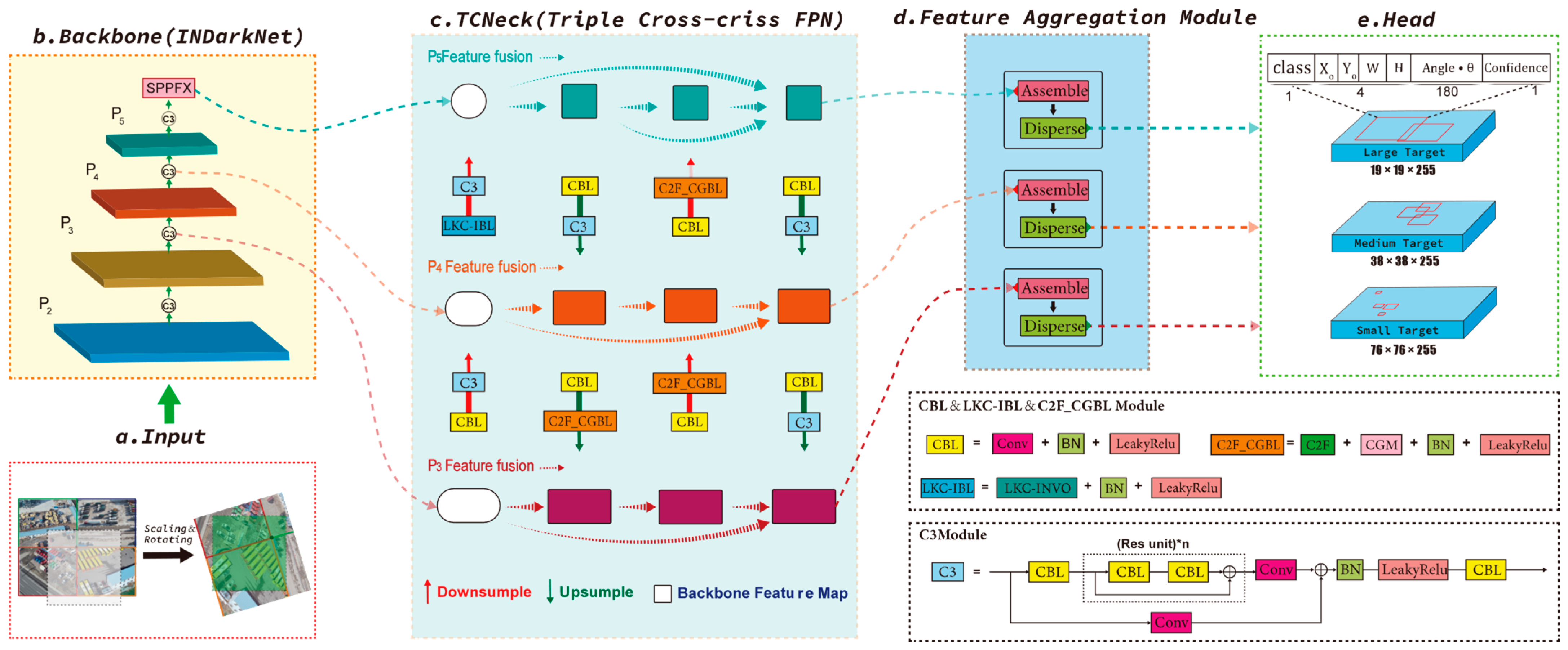
As shown in Figure 2, the ML-Det model can be roughly divided into five main parts according to the overall framework: input, backbone, neck, feature aggregation, and head.

Table A1. ML-Det network architecture details.

	From		Number	Type	Arguments
0	−1		1	Convolution	[3, 32, 6, 2, 2]
1	−1		1	Convolution	[32, 64, 3, 2, 1]
2	−1		1	BottleneckCSP	[64, 64]
3	−1		1	Convolution	[64, 128, 3, 2, 1]
4	−1		2	BottleneckCSP	[128, 128]
5	−1		1	Convolution	[128, 256, 3, 2, 1]
6	−1		3	BottleneckCSP	[256, 256]
7	−1		1	LKC–INVO	[256, 256]
8	−1		1	BottleneckCSP	[256, 512, 1, 1, 0]
9	−1		1	SPPFX	[512, 512]
10	−1		1	Convolution	[512, 256, 1, 1, 0]
11	−1		1	Up-sampling	“nearest”
12	[−1, 6]		1	Concat	-
13	−1		1	BottleneckCSP	[512, 256]
14	−1		1	Convolution	[256, 128, 1, 1, 0]
15	−1		1	Up-sampling	“nearest”
16	[−1, 4]		1	Concat	-
17	−1		1	C2F_ContextGuided	[256, 128]
18	−1		1	Convolution	[128, 128, 3, 2, 1]
19	[−1, 14]		1	Concat	-
20	−1		1	C2F_ContextGuided	[256, 256]
21	−1		1	Convolution	[256, 256, 5, 2, 1]
22	[−1, 10, 8]		1	Concat	-
23	−1		1	C2F_ContextGuided	[1024, 512]
24	−1		1	Assemble–disperse	-
25	−1		1	Convolution	[512, 512, 5, 1, 2]
26	−1		1	Up-sampling	“nearest”
27	[−1, 20, 14]		1	Concat	-
28	−1		1	BottleneckCSP	[896, 256]
29	−1		1	Assemble-Disperse	-
30	−1		1	BottleneckCSP	[256, 256, 3, 1, 1]
31	−1		1	Up-sampling	“nearest”
32	[−1, 17, 4]		1	Concat	-
33	−1		1	BottleneckCSP	[384, 128]
34	−1		1	Assemble–disperse	-
35	[34, 29, 24]		1	Detect	-
315 layers		7.91 × 106 gradients		20.1 GFLOPS	7.91 × 106 Params

In Table A1, “From” represents the input module, −1 is the default module of the previous layer, “Number” represents the number of modules, “Arguments” refers to the Param settings of the layer, [number of input channels, number of output channels, convolution kernel size, step size, fill], “-” indicates the original module Param settings, BottleneckCSP is the C3 module, Convolution is Conv.

shows the architecture etails of ML-Det network.

a. Input: The pre-processing of images. Both the mosaic augmentation algorithm and k-means algorithm that were applied to image processing have been inherited from the original oriented-YOLOv5. The mosaic augmentation algorithm as well as random flip and scale are used to generate different scenes, while rotation of the spliced, randomly generated images can further enhance the model generalization ability. The k-means algorithm is also used to automatically generate prior boxes based on the features of the dataset, which reduces the difficulty of detecting objects with different scales and aspect ratios.

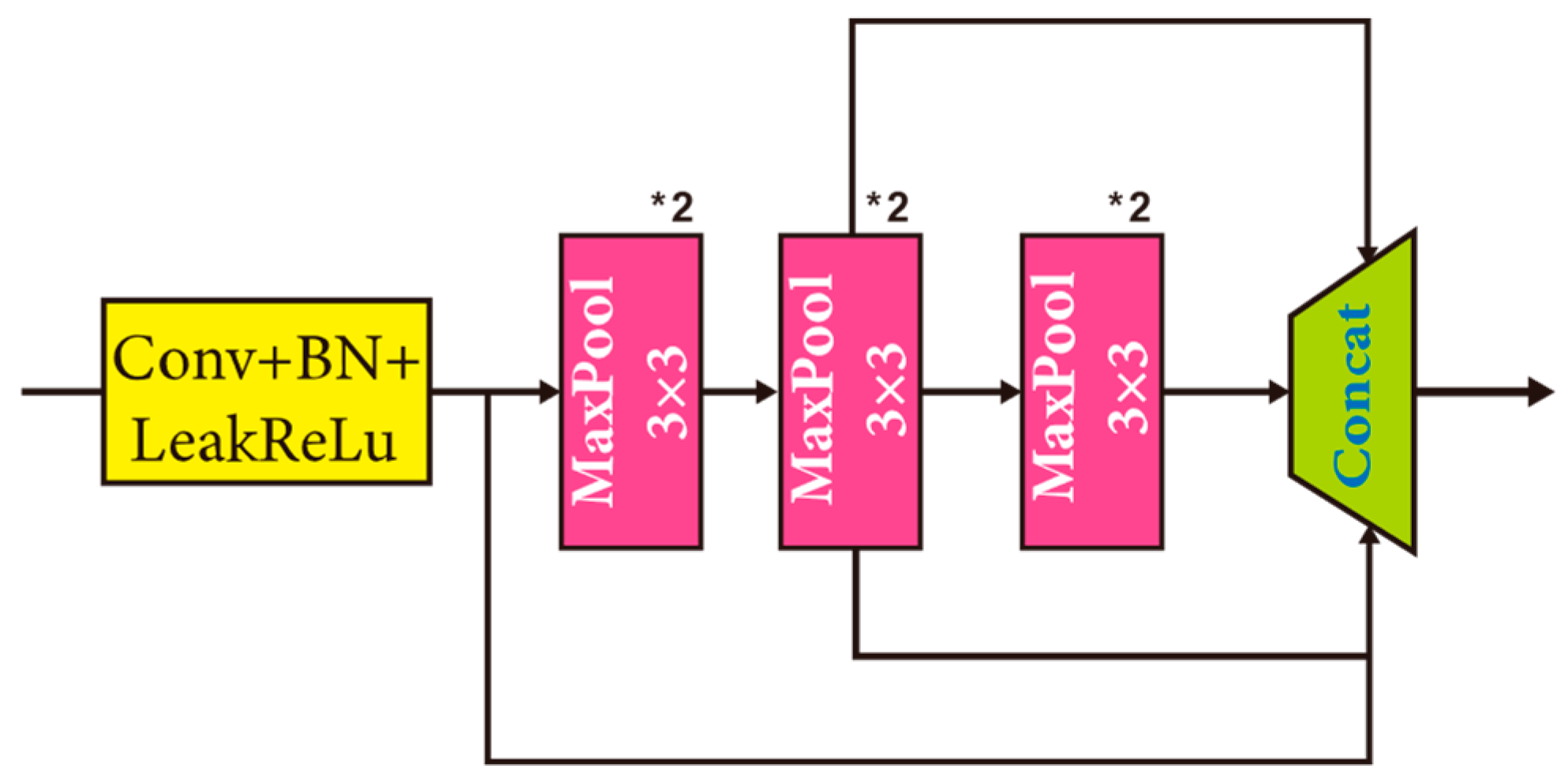
b. Backbone: The extraction of target features. The enhanced image is subjected to a stride of 2 and a kernel size of 6 for the convolution operation, allowing one to replace the original focus operation without additional computational complexity. The focus operation splits the image into four parts, reducing the spatial dimensions, but its computation can be complex. The CSPDark53 of YOLOv5 serves as our main backbone structure. With the deepening of the network, the aspect size of feature maps decreases, and the features extracted from each feature map become increasingly representative and sparse. The LKC–INVO convolution is used between {P4, P5}, which could greatly expand the model’s receptive field. The backbone and neck are connected by spatial pyramid pooling—(SPPX). The structural diagram of SPPX is shown in Figure 3. In SPPX, the 5 × 5 kernel of spatial pyramid pooling fusion (SPPF) is replaced by two 3 × 3 kernels, which increases the model depth to enhance the modeling effect under the condition of the same receptive field.

c. TCNeck: The blending of three levels of feature information. Multi-level features extracted from the backbone do not go directly to the head for target detection but need to be fused layer by layer with features from different levels first. The design of TCFPN is inspired by the BiFPN structure [12], which introduces a bidirectional residual structure but retains the single nodes that have minor influence on the model and possess a large amount of information, and fuses the single nodes in {P5}. Meanwhile, after a large number of comparison experiments, it is found that the initial feature map extracted from the backbone has rich information, and that the jump connection to the last series of feature maps can improve model precision. As the final feature map incorporates all three previous feature maps, the neck structure is referred to as TCFPN. The downsampling of TCFPN uses a convolutional kernel size of 5 to enhance the perception of large targets.

d. Feature aggregation module: The aggregation of different channel data. This module can aggregate local feature information through a mechanism of compression followed by release on the spatial scale of the feature map. Assemble can collect features on channels over a large area, while disperse can redistribute the collected features to different channels. Adding the assemble–disperse attention module to neck and head could further improve the model’s feature utilization rate by leveraging the abundant channel data.

e. Head: The output of different sizes of detection boxes. These are divided into three according to their different sizes. Non-maximum suppression (NMS) is then used for post-processing. Firstly, the candidate bounding boxes are sorted into categories according to the confidence level, with the bounding box with the largest confidence level being selected. Then, the final prediction box results are obtained through the threshold screening mechanism. The loss function of model is expressed in Equation (1).

$${\mathrm{L}\mathrm{o}\mathrm{s}\mathrm{s}}_{\mathrm{t}\mathrm{o}\mathrm{t}\mathrm{a}\mathrm{l}}={\mathrm{L}\mathrm{o}\mathrm{s}\mathrm{s}}_{\mathrm{t}\mathrm{h}\mathrm{e}\mathrm{t}\mathrm{a}}+{\mathrm{L}\mathrm{o}\mathrm{s}\mathrm{s}}_{\mathrm{o}\mathrm{b}\mathrm{j}}+{\mathrm{L}\mathrm{o}\mathrm{s}\mathrm{s}}_{\mathrm{c}\mathrm{l}\mathrm{s}}{+\mathrm{L}\mathrm{o}\mathrm{s}\mathrm{s}}_{\mathrm{b}\mathrm{o}\mathrm{x}}$$

(1)

${\mathrm{L}\mathrm{o}\mathrm{s}\mathrm{s}}_{\mathrm{t}\mathrm{h}\mathrm{e}\mathrm{t}\mathrm{a}}$, ${\mathrm{L}\mathrm{o}\mathrm{s}\mathrm{s}}_{\mathrm{o}\mathrm{b}\mathrm{j}}$, ${\mathrm{L}\mathrm{o}\mathrm{s}\mathrm{s}}_{\mathrm{c}\mathrm{l}\mathrm{s}}$, and ${\mathrm{L}\mathrm{o}\mathrm{s}\mathrm{s}}_{\mathrm{b}\mathrm{o}\mathrm{x}}$, refer to the angle loss, bounding box loss, confidence loss, and classification loss, respectively. The rotational models based on 180-degree regression with the long edge definition method all confront the boundary problem of angle θ. Therefore, we use the CSL method [41] to compute the angular loss so that the extreme angles are close to the neighbors. CSL is, in fact, a solution to implement the regression idea with classification. We use the default SiLU as the activation function, the SiLU activation function has a smooth curve when it is close to zero and can retain more input information for the scenario.

3.2. Innovation Module

3.2.1. Large Kernel Coupling Built-In Involution (LKC–INVO Convolution)

Common convolution operations are characterized by two main features: special-agnosticism and channel-specificity. The common convolution commonly has a large amount of redundant information. Involution [42] is a new convolution operation, which has the features of being channel-agnostic and space-specific in contrast with common convolution. Involution reduces Params in the model by sharing Params within the channel range and uses multiple kernel operations to enhance spatial features. However, convolution using fixed convolutional kernels still limits the visual relationship of target objects in the image and affects detection. The number of operational Params of involution in $({\mathrm{C}}^2+{\mathrm{k}}^2\mathrm{G}\mathrm{C})/\mathrm{r}$ is much lower than the ${\mathrm{k}}^2{\mathrm{C}}^2$ of common convolution. Involution is essentially a reallocation of computational power and uses the pixel region around the sample to generate the corresponding convolution kernel. This expands the receptive field to a certain extent but fails to capture the information of a wide range of different sizes of the image, limiting the precision improvement.

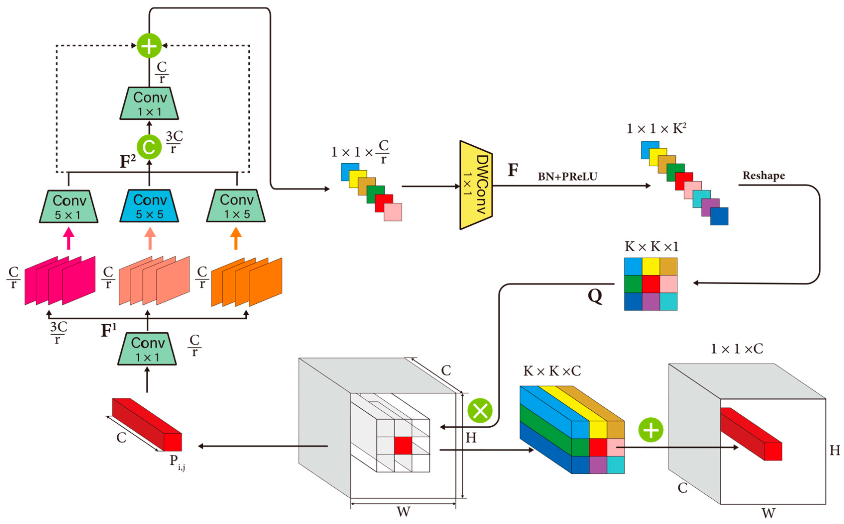
LKC–INVO convolution expands the range of the receptive field of the model and enhances the extraction ability of the model to extract high-level information by using the large kernel multi-branch coupling structure creatively on the basis of the channel invariance of involution. The large kernel multi-branch coupling structure is shown in Figure 4, employing three different convolutions of 5 × 1, 5 × 5, and 5 × 1. By concatenating the feature information extracted from the three branches, using the convolution to align the number of channels, and then adding the feature information module obtained by connecting with the residuals of ${\mathrm{C}\mathrm{o}\mathrm{n}\mathrm{v}}_{5\times 1},{\mathrm{C}\mathrm{o}\mathrm{n}\mathrm{v}}_{1\times 5}$, a large number of image features on more sizes can be combined to further improve model precision. LKC–INVO convolution also uses 7 × 7 convolution kernel size without adding excessive Params. LKC–INVO convolution is more efficient than involution and more concise than self-attention. For a set ${\mathsf{\psi }}_{\mathrm{i},\mathrm{j}}=\left\{\right(\mathrm{i},\mathrm{j}\left)\right\}$ in any one-point domain, the operational expression for LKC–INVO convolution is expressed in Equations (2)–(6).

$${\mathrm{F}}_{\mathrm{i},\mathrm{j}}^1={\mathrm{C}\mathrm{o}\mathrm{n}\mathrm{v}}_{1\times 1}({\mathrm{X}}_{{\mathsf{\psi }}_{\mathrm{i},\mathrm{j}}}),$$

(2)

$${\mathrm{F}}_{\mathrm{i},\mathrm{j}}^2=\mathrm{C}\mathrm{o}\mathrm{n}\mathrm{c}\mathrm{a}\mathrm{t}\left({\mathrm{C}\mathrm{o}\mathrm{n}\mathrm{v}}_{5\times 1}\right({\mathrm{F}}_{\mathrm{i},\mathrm{j}}^1),{\mathrm{C}\mathrm{o}\mathrm{n}\mathrm{v}}_{5\times 5}({\mathrm{F}}_{\mathrm{i},\mathrm{j}}^1),{\mathrm{C}\mathrm{o}\mathrm{n}\mathrm{v}}_{1\times 5}({\mathrm{F}}_{\mathrm{i},\mathrm{j}}^1\left)\right),$$

(3)

$${\mathrm{F}}_{\mathrm{i},\mathrm{j}}=\mathrm{D}\mathrm{W}\mathrm{C}\mathrm{o}\mathrm{n}\mathrm{v}\left({\mathrm{C}\mathrm{o}\mathrm{n}\mathrm{v}}_{1\times 1}\right({\mathrm{F}}_{\mathrm{i},\mathrm{j}}^2)+{\mathrm{C}\mathrm{o}\mathrm{n}\mathrm{v}}_{5\times 1}({\mathrm{F}}_{\mathrm{i},\mathrm{j}}^1)+{\mathrm{C}\mathrm{o}\mathrm{n}\mathrm{v}}_{1\times 5}({\mathrm{F}}_{\mathrm{i},\mathrm{j}}^1),$$

(4)

$${\mathrm{Q}}_{\mathrm{i},\mathrm{j}}=\mathsf{\varphi }({\mathrm{X}}_{{\mathsf{\psi }}_{\mathrm{i},\mathrm{j}}})={\mathrm{M}}_1·\mathsf{\sigma }\left({\mathrm{M}}_0{,\mathrm{F}}_{\mathrm{i},\mathrm{j}}\right),$$

(5)

$${\mathrm{Y}}_{\mathrm{i},\mathrm{j},\mathrm{k}}={\sum }_{(\mathrm{u},\mathrm{v})\in {∆}_{\mathrm{k}}}{\mathrm{Q}}_{\mathrm{i},\mathrm{j},\mathrm{u}+[\mathrm{k}/2],\mathrm{v}+[\mathrm{k}/2],[\mathrm{k}\mathrm{G}/\mathrm{C}]}{·\mathrm{X}}_{\mathrm{i}+\mathrm{u},\mathrm{j}+\mathrm{v},\mathrm{k}},$$

(6)

Here, the parametric number is $\mathrm{Q}\in {\mathrm{R}}^{\mathrm{k}\times \mathrm{k}\times \mathrm{H}\times \mathrm{W}\times \mathrm{G}}$, where G is the number of groups, we usually take G = 1, so $\mathrm{Q}\in {\mathrm{R}}^{\mathrm{k}\times \mathrm{k}\times \mathrm{H}\times \mathrm{W}}$. The linear transformation matrix is ${\mathrm{M}}_0\mathsf{ϵ}{\mathrm{R}}^{\mathrm{C}\times (\mathrm{c}/\mathrm{r})}$ and ${\mathrm{M}}_1\mathsf{ϵ}{\mathrm{R}}^{\mathrm{k}\times \mathrm{k}\times (\mathrm{c}/\mathrm{r})}$, the nonlinear transformation $\mathsf{\sigma }=\mathrm{P}\mathrm{r}\mathrm{e}\mathrm{l}\mathrm{u}\left(\mathrm{B}\mathrm{N}\right(\cdot \left)\right)$, r is the channel reduction ratio, the shape transformation is $\mathsf{\varphi }(\cdot )={\mathrm{M}}_1·\mathsf{\sigma }(\cdot )$, “+” is the sum operation, “∙” is the product operation, and $\mathrm{C}\mathrm{o}\mathrm{n}\mathrm{c}\mathrm{a}\mathrm{t}$ is the concatenation operation. ${\mathrm{C}\mathrm{o}\mathrm{n}\mathrm{v}}_{1\times 1},{\mathrm{C}\mathrm{o}\mathrm{n}\mathrm{v}}_{5\times 1}$ ${\mathrm{C}\mathrm{o}\mathrm{n}\mathrm{v}}_{1\times 5},$ ${\mathrm{C}\mathrm{o}\mathrm{n}\mathrm{v}}_{5\times 5}$ are convolutions with convolution kernels of 1 × 1, 5 × 1, 1 × 5, and 5 × 5 convolutions, respectively, and $\mathrm{D}\mathrm{W}\mathrm{C}\mathrm{o}\mathrm{n}\mathrm{v}$ is a depth-separable convolution with a convolution kernel size of 1 × 1.

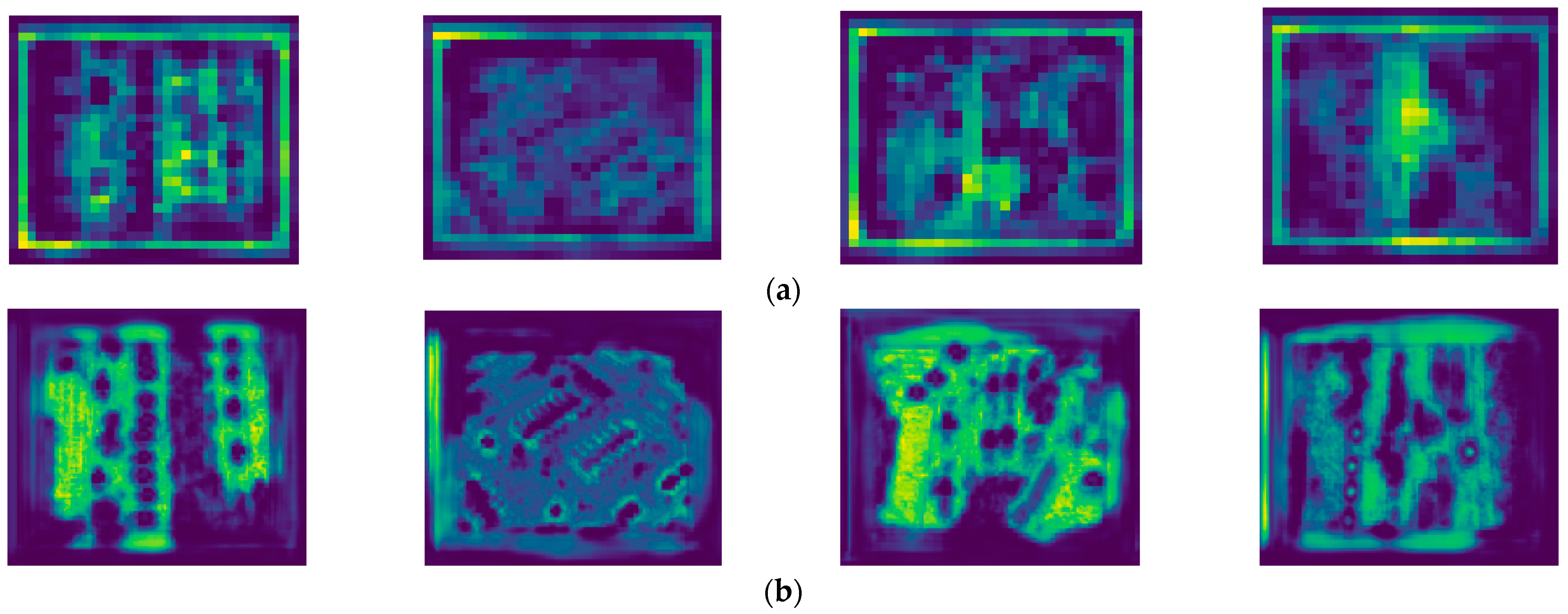
It can be seen in Figure 5 that LKC–INVO convolution can strengthen the feature acquisition ability of the model, and that the vehicle target and the background are separated from each other on the feature map, so that the general location and outline of the vehicle target can be clearly seen. Through extensive comparative experiments, we also found that it is not the case that replacing the convolution at all positions will result in a large improvement in precision, and we found that replacing some positions of the backbone with LKC–INVO can balance the performance and the degree associated with reducing the weight. As the operational volume of LKC–INVO does not grow rapidly with the convolutional kernel size, a large convolutional kernel can be selected, which makes LKC–INVO convolution more suitable for the detection of large target objects.

3.2.2. C2F_ContextGuided Context-Perception Module

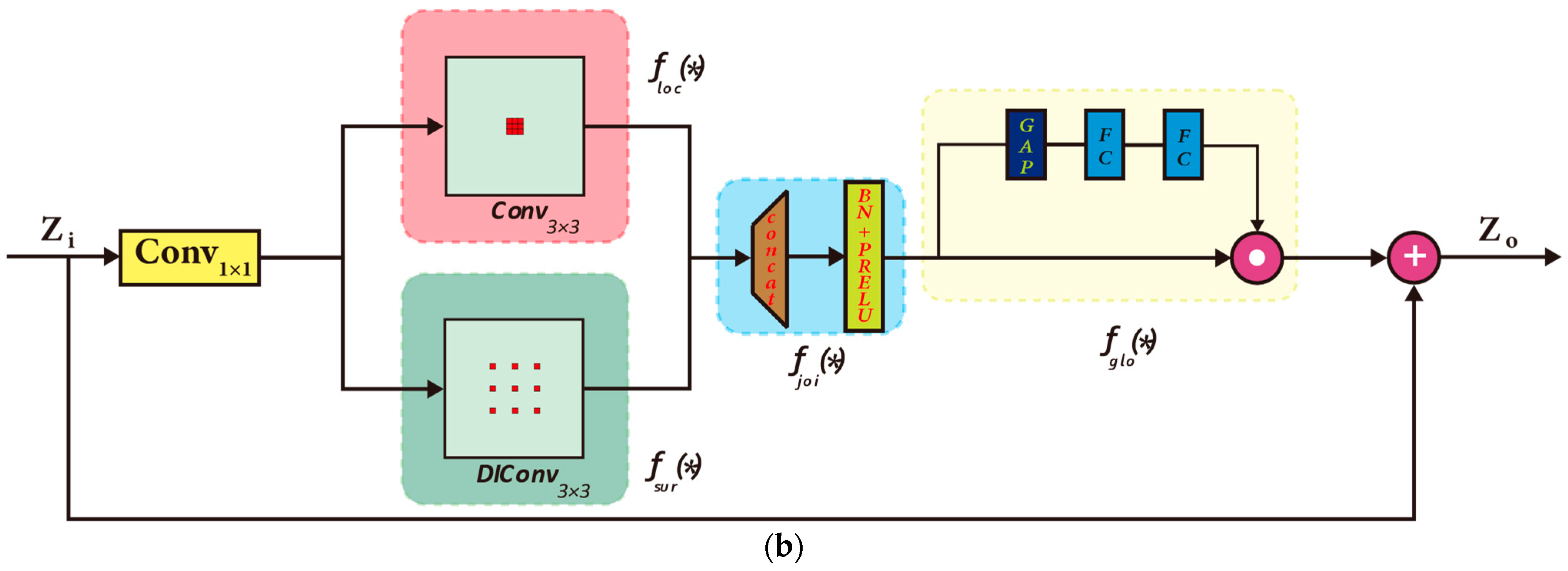
The C2F module is used in YOLOv8, which synthesizes the design ideas of the C3 module and the efficient layer-wise attention network (ELAN) [43] to allow the model to be lightweight and to obtain rich gradient flow information. The C2F module uses the split operation to divide the feature map into two sub-feature maps along the channel dimension. The convolution operation in the branch is eliminated, and more jump connections are added so that the model obtains abundant gradient flow information, which strengthens the feature information of the model while keeping it lightweight. The ContextGuided module [41] can simulate the human visual system, which needs contextual information to perceive different scenes and combine contextual information from different regions. The module first uses ${\mathrm{C}\mathrm{o}\mathrm{n}\mathrm{v}}_{1\times 1}$ to change the number of channels to reduce the computational complexity. Then, the local feature information ${\mathrm{f}}_{\mathrm{l}\mathrm{o}\mathrm{c}}$ of the model is learned using standard convolution ${\mathrm{C}\mathrm{o}\mathrm{n}\mathrm{v}}_{3\times 3}$ and the wide range of surrounding contextual letter information ${\mathrm{f}}_{\mathrm{s}\mathrm{u}\mathrm{r}}$ is obtained using null convolution ${\mathrm{D}\mathrm{I}\mathrm{C}\mathrm{o}\mathrm{n}\mathrm{v}}_{3\times 3}$ with a dilatation rate (dilatation rate) of 2. This is undertaken to help the model to understand more complex scenario information. Next, the joint feature information is obtained by combining the local information with the information from the surrounding context by concatenation, using batch normalization (BN) and the SiLU activation function to further improve the feature representation and obtain the joint feature information ${\mathrm{f}}_{\mathrm{j}\mathrm{o}\mathrm{i}}$. However, this operation of feature association is only a shallow combination of information. To enhance features using the entire input image, we use global average pooling (GAP) to obtain global information about the entire feature map. The global contextual feature information is then refined using two fully connected (FC) layers. FC contains the scaling of channel dimensions, which serves to recalibrate the joint feature information to reach the global information ${\mathrm{f}}_{\mathrm{g}\mathrm{l}\mathrm{o}}$. Finally, the residuals are then used to connect the inputs to obtain the output features. The schematic diagram of the C2F_ContextGuided module is shown in Figure 6. The C2F_ContextGuided module can enhance the advantages of these, and only requires replacing all bottlenecks in the C2F module with the CG_Bottleneck module. The CG_Bottleneck module can send a large amount of image context information back to the C2F module, which then feeds the information into the C2F module through abundant gradient flow to the model for decision making, thus improving the detection precision of the model. The operational expression for the C2F_ContextGuided module is expressed in Equations (7)–(9).

$${\mathrm{Z}}_{1,\mathrm{o}}={\mathrm{f}}_{\mathrm{g}\mathrm{l}\mathrm{o}}\left({\mathrm{f}}_{\mathrm{j}\mathrm{o}\mathrm{i}}\right({\mathrm{f}}_{\mathrm{l}\mathrm{o}\mathrm{c}}\left({\mathrm{Z}}_{1,\mathrm{i}}\right)+{\mathrm{f}}_{\mathrm{s}\mathrm{u}\mathrm{r}}\left({\mathrm{Z}}_{1,\mathrm{i}}\right)\left)\right)+{\mathrm{Z}}_{1,\mathrm{i}},$$

(7)

$${\mathrm{Z}}_{2,\mathrm{o}}={\mathrm{f}}_{\mathrm{g}\mathrm{l}\mathrm{o}}\left({\mathrm{f}}_{\mathrm{j}\mathrm{o}\mathrm{i}}\right({\mathrm{f}}_{\mathrm{l}\mathrm{o}\mathrm{c}}\left({\mathrm{Z}}_{1,\mathrm{o}}\right)+{\mathrm{f}}_{\mathrm{s}\mathrm{u}\mathrm{r}}\left({\mathrm{Z}}_{1,\mathrm{o}}\right)\left)\right)+{\mathrm{Z}}_{2,\mathrm{i}},$$

(8)

$${\mathrm{X}}_{\mathrm{o}}=\mathrm{C}\mathrm{B}\mathrm{L}\left(\mathrm{C}\mathrm{o}\mathrm{n}\mathrm{c}\mathrm{a}\mathrm{t}\right({\mathrm{Z}}_{1,\mathrm{o}}+{\mathrm{Z}}_{2,\mathrm{o}}+\mathrm{S}\mathrm{p}\mathrm{l}\mathrm{i}\mathrm{t}\left(\mathrm{C}\mathrm{B}\mathrm{L}\right({\mathrm{X}}_{\mathrm{i}}\left)\right)),$$

(9)

where split is the dimensional segmentation function, ${\mathrm{f}}_{\mathrm{l}\mathrm{o}\mathrm{c}}$ is the extraction of local feature operations, ${\mathrm{f}}_{\mathrm{s}\mathrm{u}\mathrm{r}}$ is the extraction of surrounding features operation, “+” represents the residual sum operation, and $\mathrm{C}\mathrm{B}\mathrm{L}$ is the convolution normalization and activation function transformation. ${\mathrm{X}}_{\mathrm{i}}$ and ${\mathrm{X}}_{\mathrm{o}}$ are the global inputs and outputs, respectively. ${\mathrm{Z}}_{1,\mathrm{i}}$, ${{\mathrm{Z}}_{2,\mathrm{i}}{\mathrm{a}\mathrm{n}\mathrm{d}\mathrm{Z}}_{1,\mathrm{o}},\mathrm{Z}}_{2,\mathrm{o}}$ are the local CG_ inputs and outputs on the bottleneck, respectively.

3.2.3. Assemble–Disperse Attention Module

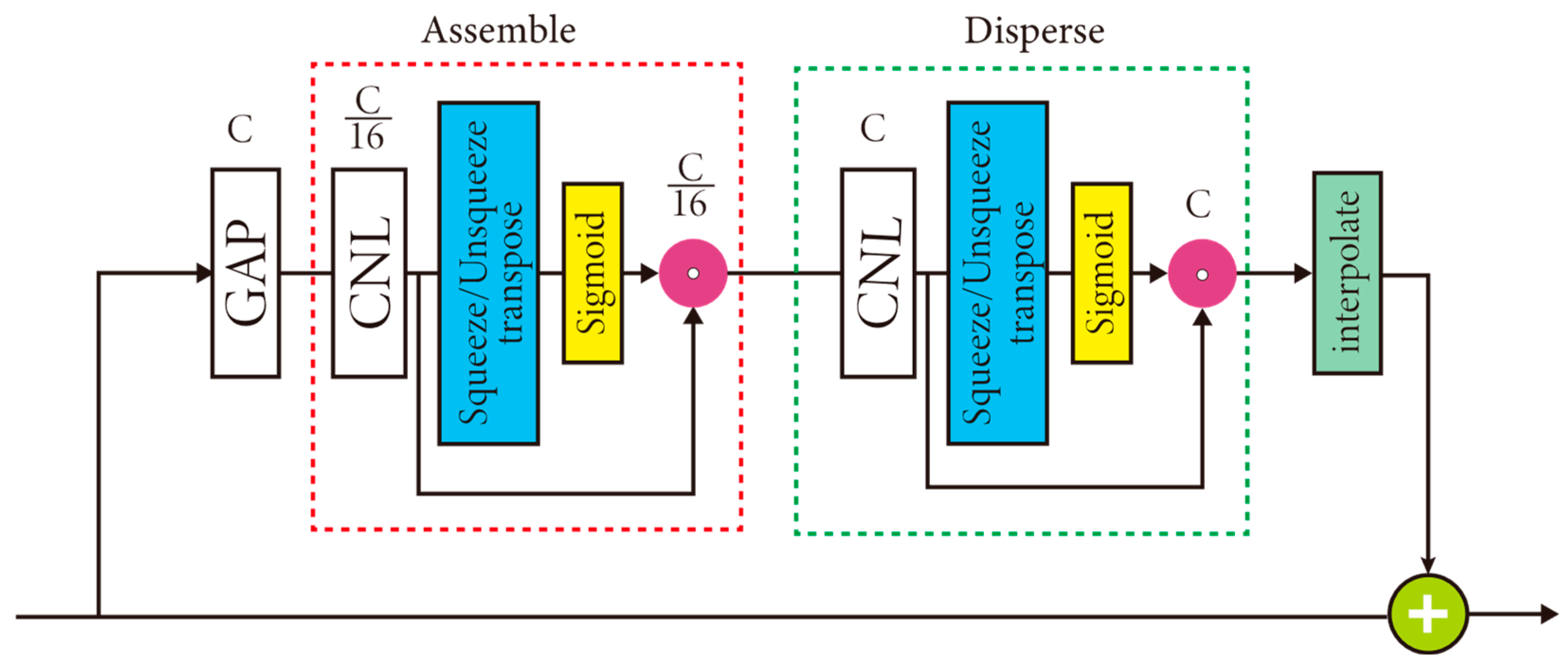
The assemble–disperse module takes its cue from SE attention [30], which also aggregates local feature information within a range through a mechanism of compression followed by release on the spatial scale of the feature map. Assemble can collect features on channels over a large area, while disperse can redistribute the collected features to different channels. Figure 7 shows the schematic diagram of the assemble–disperse module. The specific steps are as follows: first, the global average pooling (GAP) is performed on the spatial dimension [w,h] to obtain the features on all channels without additional operations on the spatial range. In the assemble stage, using convolution with convolution kernel size 1, the number of feature channels is compressed to 1/16 times the original one, aggregating the local feature information of different channels, followed by a layer normalization operation to improve the model stability. Feature activation is performed with the SiLU activation function, and transpose-and-squeeze and sigmoid operations are used to achieve full channel interaction in the one-dimensional convolution over the channels and to redistribute the weights in the one-dimensional convolution dimension. A dropout operation is used between assemble and disperse to prevent excessive increase in the number of Params. In the disperse stage, a convolution with a convolution kernel size of 1 is used to extend the number of feature channels to 16 times the original number, keeping it the same as the number of input channels, followed by a layer normalization operation to keep the gradient stable. The feature activation is performed with the SiLU activation function, using transpose-and-squeeze as well as sigmoid operations to achieve full channel interaction in one-dimensional convolution over the channels and in one-dimensional convolutional dimensions, redistributing the weights. Finally, the spatial dimensions are recovered with interpolate operation, and is further linked with the original input using residual branch. With this series of operations, assemble–disperse, the information on the channels can be well redistributed to aggregate different feature information.

4. Experiment

4.1. Param Setting

Table 1. Software and hardware environment.

Environmental Types	Environmental Parameters
Hardware	CPU	Intel(R) Xeon(R) Gold 5218
	Memory	32G
	GPU	NVIDIA 4090
	Video memory	24G
Software	System	Win10
	Graphics card driver	CUDA 11.3, CUDNN 8.2
	Deep learning framework	Pytorch 1.10, python 3.8, VS (2019), Opencv, MMRotate

and

Table 2. Training Params.

Training Params	Param Values
Batch size	8
Weight decay	0.0005
Momentum	0.9
Non-Maximum Suppression (NMS)	0.5
Learning rate	0.01
Data augmentation method	Mosaic
Optimizer	SGD

list the environment and training Params, respectively. All experiments were set according to the above parameters, we set it to 150 rounds, but most models converge around 100 rounds, so if the model converges early, the highest precision at convergence is used as the final data. The MMrotate toolbox has a large number of well-integrated rotating box-based detection models, we compare all of the initial Params uniformly for comparison experiments. As the precision of the stochastic gradient descent (SGD) optimizer fluctuates, we will test it 3 times consecutively and take the arithmetic average of the 5 times data as the final value of mAP.

4.2. Evaluation Indicators

Table 3. Confusion matrix.

		Actual
		Positive	Negative
Prediction	Positive	TP	FP
	Negative	FN	TN

shows the confusion matrix. The model precision evaluation indicators include the following: precision (P), recall (R), average precision (AP), mean average precision (mAP), true positives (TP), false positives (FP), false negatives (FN), true negatives (TN).

${\mathrm{A}\mathrm{P}}_{07}$ and ${\mathrm{A}\mathrm{P}}_{12}$ are the APs that are respectively obtained in the manner that the VOC2007 and VOC2012 indicators are computed. ${\mathrm{A}\mathrm{P}}_{07}$ is computed by calculating the total area of the column enclosed by 11 discrete Rs with their corresponding Ps. ${\mathrm{A}\mathrm{P}}_{07}$ calculates the area of the irregular graph surrounded by the smooth curve and the R axis. $\mathrm{m}\mathrm{A}\mathrm{P}$ refers to the mean value of the detection precision of different kinds of targets. mAP is divided into ${\mathrm{m}\mathrm{A}\mathrm{P}}_{07}$ and ${\mathrm{m}\mathrm{A}\mathrm{P}}_{12}$ according to the different calculation methods of the VOC2007 and VOC2012 indicators, and, in this paper, we adopt the calculation method of VOC2012 by default. When detecting multiple classes of targets, AP is calculated for each class and then mAP is obtained by calculating the arithmetic mean of all AP values. mAP is a composite measure of the average precision of the detected targets, where m denotes the number of classes of targets in the dataset. Equations (10)–(13) express the definitions of P, R, ${\mathrm{A}\mathrm{P}}_{07}$ and AP.

$$\mathrm{P}={\displaystyle \frac{\mathrm{T}\mathrm{r}\mathrm{u}\mathrm{e} \mathrm{P}\mathrm{o}\mathrm{s}\mathrm{i}\mathrm{t}\mathrm{i}\mathrm{v}\mathrm{e}\mathrm{s}}{\mathrm{A}\mathrm{l}\mathrm{l} \mathrm{P}\mathrm{o}\mathrm{s}\mathrm{t}\mathrm{i}\mathrm{v}\mathrm{e}\mathrm{D}\mathrm{e}\mathrm{t}\mathrm{e}\mathrm{c}\mathrm{t}\mathrm{i}\mathrm{o}\mathrm{n}\mathrm{s}}}={\displaystyle \frac{\mathrm{T}\mathrm{P}}{\mathrm{T}\mathrm{P}+\mathrm{F}\mathrm{P}}}$$

(10)

$$\mathrm{R}={\displaystyle \frac{\mathrm{T}\mathrm{r}\mathrm{u}\mathrm{e} \mathrm{P}\mathrm{o}\mathrm{s}\mathrm{i}\mathrm{t}\mathrm{i}\mathrm{v}\mathrm{e}\mathrm{s}}{\mathrm{A}\mathrm{l}\mathrm{l} \mathrm{G}\mathrm{r}\mathrm{o}\mathrm{u}\mathrm{n}\mathrm{d}\mathrm{T}\mathrm{r}\mathrm{u}\mathrm{t}\mathrm{h}\mathrm{s}}}={\displaystyle \frac{\mathrm{T}\mathrm{P}}{\mathrm{T}\mathrm{P}+\mathrm{F}\mathrm{N}}}$$

(11)

$${\mathrm{A}\mathrm{P}}_{07}={\displaystyle \frac{1}{11}}\sum \mathrm{M}\mathrm{a}\mathrm{x}\left(\mathrm{P}\right(\mathrm{r}\left)\right),{\mathrm{m}\mathrm{A}\mathrm{P}}_{07}={\displaystyle \frac{\sum {\mathrm{A}\mathrm{P}}_{07}}{\mathrm{m}}},\mathrm{r}\in \left\{\mathrm{0,0.1},...,1\right\}$$

(12)

$$\mathrm{A}\mathrm{P}={\mathrm{A}\mathrm{P}}_{12}={\int }_0^1\mathrm{P}\left(\mathrm{r}\right)\mathrm{d}\mathrm{r},\mathrm{m}\mathrm{A}\mathrm{P}={\mathrm{m}\mathrm{A}\mathrm{P}}_{12}={\displaystyle \frac{\sum {\mathrm{A}\mathrm{P}}_{12}}{\mathrm{m}}},\mathrm{r}\in \left\{0,\mathrm{r}\left(0\right),...,\mathrm{r}\left(\mathrm{k}\right),1\right\}$$

(13)

The size assessment indicator of the model is mainly Param, which is mainly used to measure the size of the model (computational space complexity).

The model’s real-time evaluation indicators include the following: frames per second (FPS), giga floating-point operations per second (GFLOPS). FPS refers to the number of image frames that can be processed per second. The more frames per second, the smoother the displayed action will be. Generally, the minimum to avoid poor movement is 30. The faster the inferencing, the better the real-time performance and the more scenarios it can be applied to. GFLOPS refers to the number of billion floating point operations per second, which can be interpreted as the amount of computational time complexity, and is generally used to measure algorithmic complexity.

4.3. Dataset

4.3.1. MiVehicle Dataset

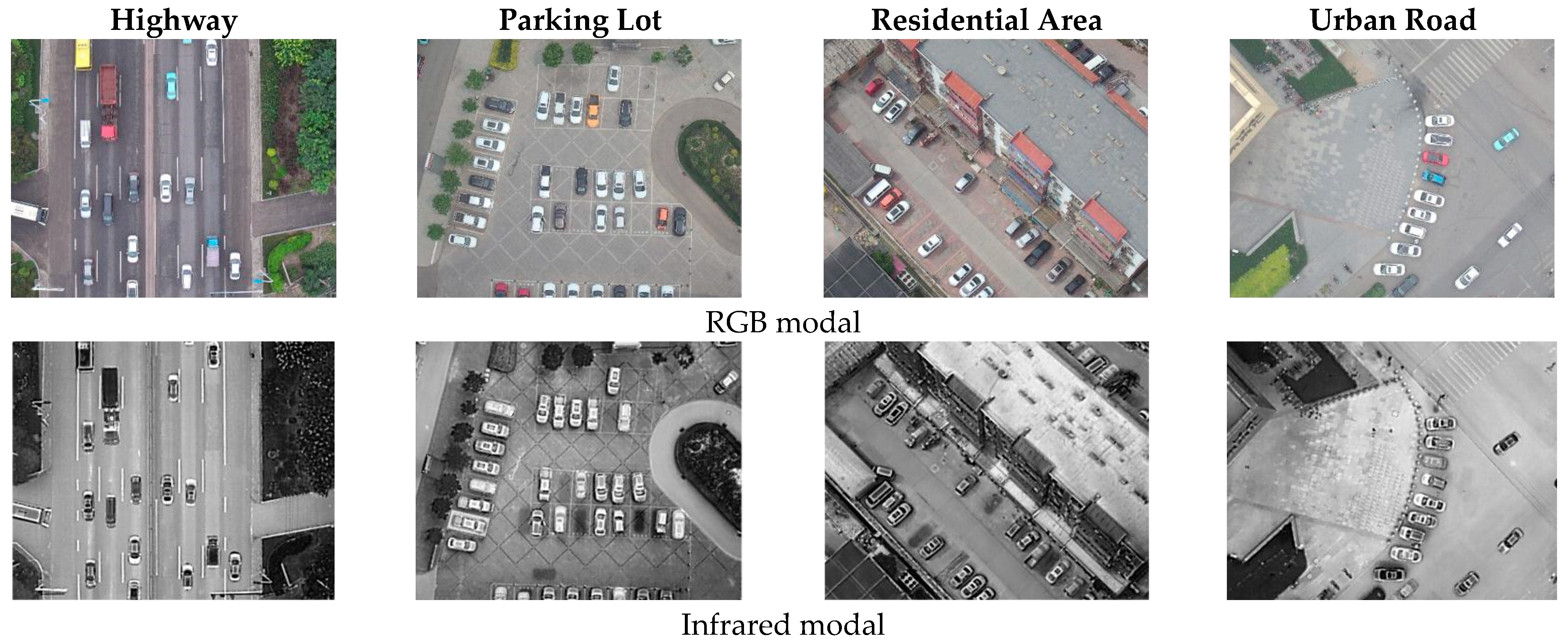
MiVehicle is a self-constructed dataset drawn from the DroneVehicle dataset [7]. DroneVehicle is a large RGB-T dataset captured by Tianjin University with drones that is aggregated to include the following five different vehicles labeled with oriented bounding boxes: car, truck, bus, freight car and van.

Table 4. The specific information of the DroneVehicle dataset.

Size	#Images	Modality	#Labels/Categories	Oriented BB	Year
840 × 712	56,878	R + I	190.6 k	√	2021
Categories	Car (R/I)	Truck (R/I)	Bus (R/I)	Van (R/I)	Freight Car (R/I)
5	389,779/428,086	22,123/25,960	15,333/16,590	11,935/12,708	13,400/17,173

lists the specific information of the DroneVehicle dataset. Figure 8 shows the MiVehicle sample.

The advanced algorithm UA-CMDet [7], proposed by the authors, also has an mAP of 64.01%. Because of the uneven distribution among the individual vehicle samples, we sampled 3000 infrared and visible light images, prioritized the vehicle types with small numbers and segmented them according to the ratio of 8:1:1 to obtain 2400 for the training set, 300 for the validation set, and 300 for the test set. Figure 9 shows the comparison for each vehicle proportion between the MiVehicle and the DroneVehicle datasets.

4.3.2. UCAS_AOD Dataset

UCAS_AOD dataset [8] was collected, labeled and released by the Pattern Recognition Laboratory at the University of Chinese Academy of Sciences. Figure 10 presents the UCAS_AOD sample. The image source is Google Earth’s satellite high-definition remote sensing image. The dataset contains two types of vehicles, aircraft and vehicles, and the target objects are uniformly distributed on the images. There are 510 vehicle images with a total of 7114 vehicle targets at a resolution of 1280 × 685. There are 1000 aircraft images with a total of 7482 aircraft targets and with a resolution of 1280 × 659. The dataset provides both horizontal and rotated box labeling formats. We divided the dataset into 755 training, 302 validation and 453 test sets in the ratio of 5:2:3 and kept the original image size.

4.3.3. DOTA Dataset

The DOTA dataset [5] is widely used in the evaluation of rotating target detection, this paper uses DOTAv1.0 version. Most of the images of the DOTA dataset come from Google Earth, with some others deriving from images taken by the JL-1 and GF-2 satellites and from China Resources Satellite (CRS) data.

Table 5. Specific information of the DOTA dataset.

Size	#Images	Modality	#Labels/Categories	Oriented BB	Year
12,029 × 5014	2806	R	12.5 k	√	2018
Categories	Plane (PL)	Ship (SP)	Storage tank (ST)	Baseball diamond (BD)	Tennis court (TC)
15	Swimming pool (SP)	Athletic field (GTF)	Harbor (HA)	Bridge (BR)	Large vehicle (LV)
	Small vehicle (SV)	Helicopter (HC)	Roundabout (RA)	Soccer ball field (SBF)	Basketball court (BC)

lists the specific information of the DroneVehicle dataset. Figure 11 shows the DOTA sample.

Due to the large size, we segmented the original dataset according to 1024 × 1024, gap = 200, ration = 1.0, with single scale training, and obtained a total of 15,749 sheets for the training set and 5297 sheets for the validation set. We used the training set and test set together, totaling 21,046 sheets to train the model and using the validation set to validate it. We then submitted the test results to the DOTA official website for online testing.

4.4. Ablation Experiment

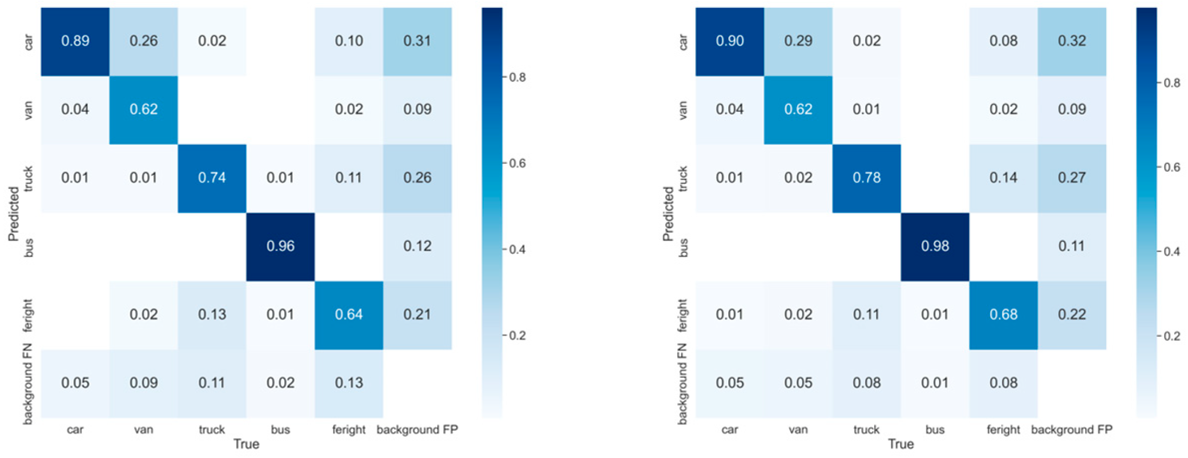
In order to more intuitively visualize the performance status of the model after the addition of the innovation module, we conducted ablation experiments on the DroneVehicle data infrared modal. Buses are characterized by high precision due to their distinctive appearance. Cars exhibit slightly reduced precision due to the model being trained with the MiVehicle dataset rather than the DroneVehicle dataset. The three vehicle types, truck, van, and freight car, show a more significant improvement in precision. Figure 12 and Figure 13 compare the detection differences and confusion matrices of YOLOv5s-obb and ML-Det, respectively.

As can be seen from

Table 6. Comparison of ablation experiments.

Methods	Baseline	Impro1	Impro2	Impro3	ML-Det
TCFPN	-	√	√	√	√
LKC-INVO	-	-	√	√	√
C2F_ContextGuided	-	-	-	√	√
Assemble–disperse	-	-	-	-	√
APCar (%)	87.44	87.80	88.45	88.31	88.02
APVan (%)	60.35	63.61	62.07	64.16	64.10
APTruck (%)	74.49	76.42	78.56	76.68	77.72
APBus (%)	95.91	97.50	97.15	97.35	97.80
APFreight car (%)	61.29	64.03	67.57	66.70	67.96
mAP (%)	75.90	77.87	78.76	78.64	79.12
Param (M)	7.78	9.76	8.50	7.87	7.91
GFLOPS	17.7	22.3	21.3	20.1	20.1

Baseline is YOLOv5s-obb, where “-“ means that the model does not use the module and “√” means that the model uses the module.

, adding TC-FPN feature fusion structure significantly enhances detection precision due to its ability to efficiently fuse three feature maps of different scales. Specifically, the accuracy improvements for vans, trucks, and freight cars were found to be 3.62%, 1.93%, and 2.74%, respectively. However, this comes with a Param increase of 1.97 M and a computational complexity increase of 4.55 GLOPS. The LKC–INVO expands the model’s receptive field and enhances its ability to extract high-level information, leading to notable accuracy gains of 4.07% and 6.28% for trucks and freight cars, respectively. The Param remains relatively unchanged compared with the baseline. The C2F_ContextGuided module integrates contextual information to improve detection precision while decreasing the model’s Param, maintaining computational complexity. The assemble–disperse module consolidates additional local feature information, resulting in further performance enhancement over the baseline model. The accuracy for vans, trucks, and freight cars increases by 3.75%, 3.23%, and 6.67%, respectively, and mAP improves 3.22%. The Param increment of 0.13 M is acceptable. The increase in computational complexity by 2.4 GFLOPS is due to the use of additional features for detection.

4.5. Results on Dataset

4.5.1. Results on MiVehicle Dataset

In this dataset, in order to guarantee the light weight of the model, ResNet50+FPN structure was selected by default for the backbone and neck, except for RoI Transformer with Swin-Tiny + FPN, RTMDet with CSPDarkNext + FPN, and InDarkNet + TCFPN. I denotes visible images and R denotes infrared images. The best results are also bolded. Uniform data tests were performed according to the input image size defaulted to 864 × 736. We tested a total of 11 different methods, including CFA [44], Gliding vertex [45], Oriented-Reppoints [46], ReDet [47], S2Anet [48], O-RCNN [49], RoI Transformer* [50], Faster R-CNN-O [51], RTMDet-S [52], YOLOv5s-obb, and ML-Det.

As clearly shown in

Table 7. Comparison of indicators for different state-of-the-art models on the MiVehicle dataset.

Methods	Modality	AP (%)					mAP (%)
		Car	Van	Truck	Bus	Freight Car
CFA	R	80.6	63.5	59.4	91.7	52.6	69.56
	I	86.7	63.9	70.7	95.4	62.4	75.82
Gliding vertex	R	80.0	58.3	55.0	90.7	46.0	66.02
	I	86.6	60.7	73.0	95.0	56.1	74.27
Oriented-Reppoints	R	82.2	62.7	60.4	92.6	55.5	70.68
	I	88.7	67.1	77.6	97.3	64.5	79.05
ReDet	R	76.6	52.4	49.1	87.6	39.5	61.03
	I	86.5	61.2	69.2	94.9	58.8	74.10
S2Anet	R	80.9	61.6	58.9	93.7	53.3	69.67
	I	88.0	64.9	72.3	97.1	65.4	77.53
O-RCNN	R	82.0	62.5	58.8	95.1	52.1	70.09
	I	87.9	64.1	77.5	97.6	64.5	78.34
RoI Transformer	R	81.8	59.6	59.9	93.6	48.0	68.58
	I	86.6	62.1	74.3	97.0	61.9	76.38
Faster R-CNN-O	R	81.0	58.3	54.4	88.5	48.4	66.09
	I	86.7	67.0	69.2	94.1	56.8	74.76
RTMDet-S	R	80.5	58.1	67.4	94.8	58.1	70.97
	I	87.3	65.8	77.5	98.4	68.0	79.43
YOLOv5s-obb	R	80.6	54.2	63.3	94.3	50.4	68.70
	I	87.4	60.4	74.5	96.0	61.3	75.90
ML-Det (ours)	R	82.3	57.8	61.0	95.3	51.4	70.44
	I	88.0	64.1	77.7	97.8	68.0	79.12

Bolded in blue are the optimal metrics for each category of visible image, bolded in red are the optimal metrics for each category of infrared image, and the optimal metrics for model Params are bolded in blue.

, it can be seen that, on visible light images, ML-Det is detected on five different vehicle targets: car, truck, bus, freight car and van. Visible image test results show a total of two kinds of targets: those that achieved the best detection results, with respective Aps of 82.3.7%, 95.3%, respectively, and infrared image test results which show that trucks and freight cars have achieved the best detection results, with Aps of 77.7% and 68.0%, respectively. These results clearly demonstrate the superiority of the algorithm proposed in this paper. Figure 14 illustrates the effect of the actual detection of two pairs of infrared and visible light pictures, detection for the infrared image is clearly better than that for the visible light image. In scenario ①, the trucks are traveling side by side in the lower right region on the visible image, and, due to the dim light, O-RCNN, S²Anet, and Gliding vertex misdetect the trucks as freight cars, whereas ML-Det and RTMDet-S are highly resistant to interference and detect the trucks. The small car below on the IR image is parked at the edge of the road, the square object next to it is easily misdetected as a car, while the vehicle target is not misdetected by Gliding vertex, RTMDet-S, and ML-Det. In scenario ②, two trucks are parked by the house in the lower left part of the visible image, while the house roof and the trucks are similar in appearance and features, meaning that they are easily misdetected as trucks and are only correctly boxed out by S²Anet. The trucks are densely lined up and the overlapping of prediction frames is more common. The probability of misdetection increases on the infrared image, and ML-Det correctly detects the truck target, but is prone to misdetecting the freight car as a van.

4.5.2. Results on UCAS_AOD Dataset

The model backbone adopts mostly lightweight R50, CSPDarkNet, etc., where R50 stands for Resnet50. We use VOC2012 indicators, as they yield higher results than VOC2007 indicators, which is due to the different computational mechanisms of AP. As the original data species vehicle and plane images are labeled separately and the image sizes are different, we defaulted to using a 1024 × 1024 size as the input size for testing model Params.

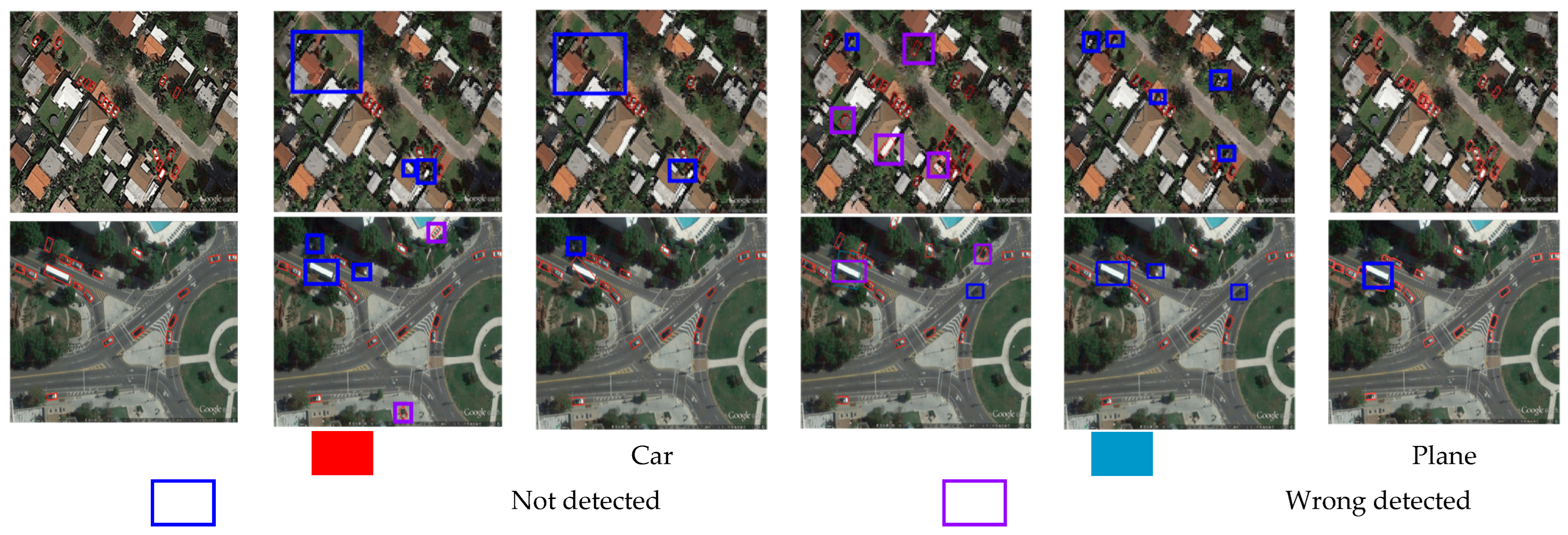
From

Table 8. Comparison of indicators for different advanced models on UCAS_AOD dataset.

Methods	Backbone	AP (%)		$\mathbf{m}\mathbf{A}\mathbf{P}$ (%)	Params (M)
		Car	Plane
Oriented Reppoints	R50-FPN	88.7	97.9	93.29	36.60
Rotated RetinaNet	R50-FPN	84.2	93.8	89.02	36.15
Gliding vertex	R50-FPN	88.9	94.7	91.79	41.13
YOLOv5s-obb	CSPDarkNet-PAFPN	89.0	98.9	93.96	7.78
S2ANet	R50-FPN	90.9	95.3	93.00	38.54
O-RCNN	R50-FPN	89.8	96.6	93.23	41.13
ReDet	R50-ReFPN	88.3	96.2	92.25	31.55
RoI Transformer	Swin tiny-FPN	90.0	97.1	93.51	58.66
RTMDet-S	CSPNeXt-PAFPN	91.1	97.8	94.45	8.86
Rotated FCOS	R50-FPN	87.2	98.2	92.69	31.89
Faster R-CNN-O	R50-FPN	89.5	95.1	92.27	41.12
ML-Det (ours)	INDarkNet-TCFPN	91.3	99.3	95.25	7.91

The optimal indicators have been bolded and reddened.

, we can see that ML-Det leads all other algorithms in both vehicle and plane detection, with their precision APs of 91.3% and 99.3%, respectively, for a total mAP of 95.25%. We then compared the test plot results for a total of six different rotating target detectors, O-RCNN, S²ANet, Faster R-CNN-O, Gliding vertex, and the ML-Det proposed in this paper. As can be seen from the detection maps in Figure 15, the vehicle targets are generally small in scenario ①, and Gliding vertex and Faster R-CNN-O show serious missed detection, while ML-Det and S²ANet detect well. In the upper-left region of scenario ②, the vehicles and the background are fused, which is easily ignored during the detection process. O-RCNN and S²ANet do not detect targets in this region, while Faster R-CNN-O and ML-Det can better separate targets from the background. In scenario ③, a large number of small vehicles are blended around a single large vehicle, which interferes with the detector’s judgment. Faster R-CNN-O mistakenly detects the large vehicle as a plane, and only S²ANet detects the large vehicles. ML-Det also shows many missed detections, but all other vehicles are detected correctly.

4.5.3. Results on DOTA Dataset

We compare different advanced algorithms on DOTA v1.0 dataset without using multi-scale methods during both training and testing, and by default, we use the pre-trained ResNet from the COCO dataset as the backbone network. All models were trained with single-scale training methods, and they are all the results of the DOTA online system test. The model backbones were pre-trained with the COCO dataset. As these large backbones, ResNet101 and ResNet152, do not meet the lightweight requirements, they were not used for the comparison experiments. Therefore, most models elected to use ResNet50 as their backbones. The input image size was set according to the actual size of the cropped image (1024 × 1024).

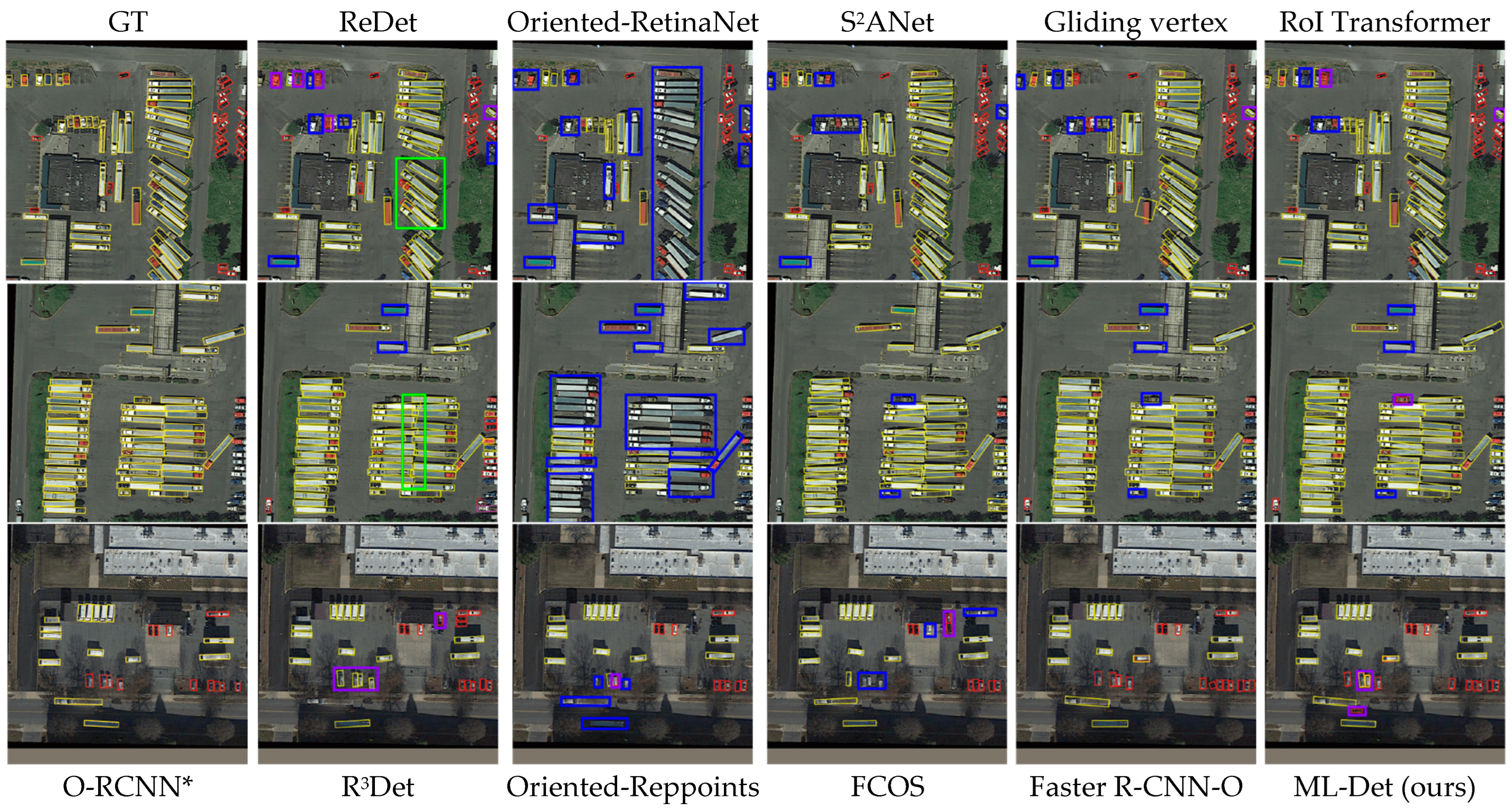
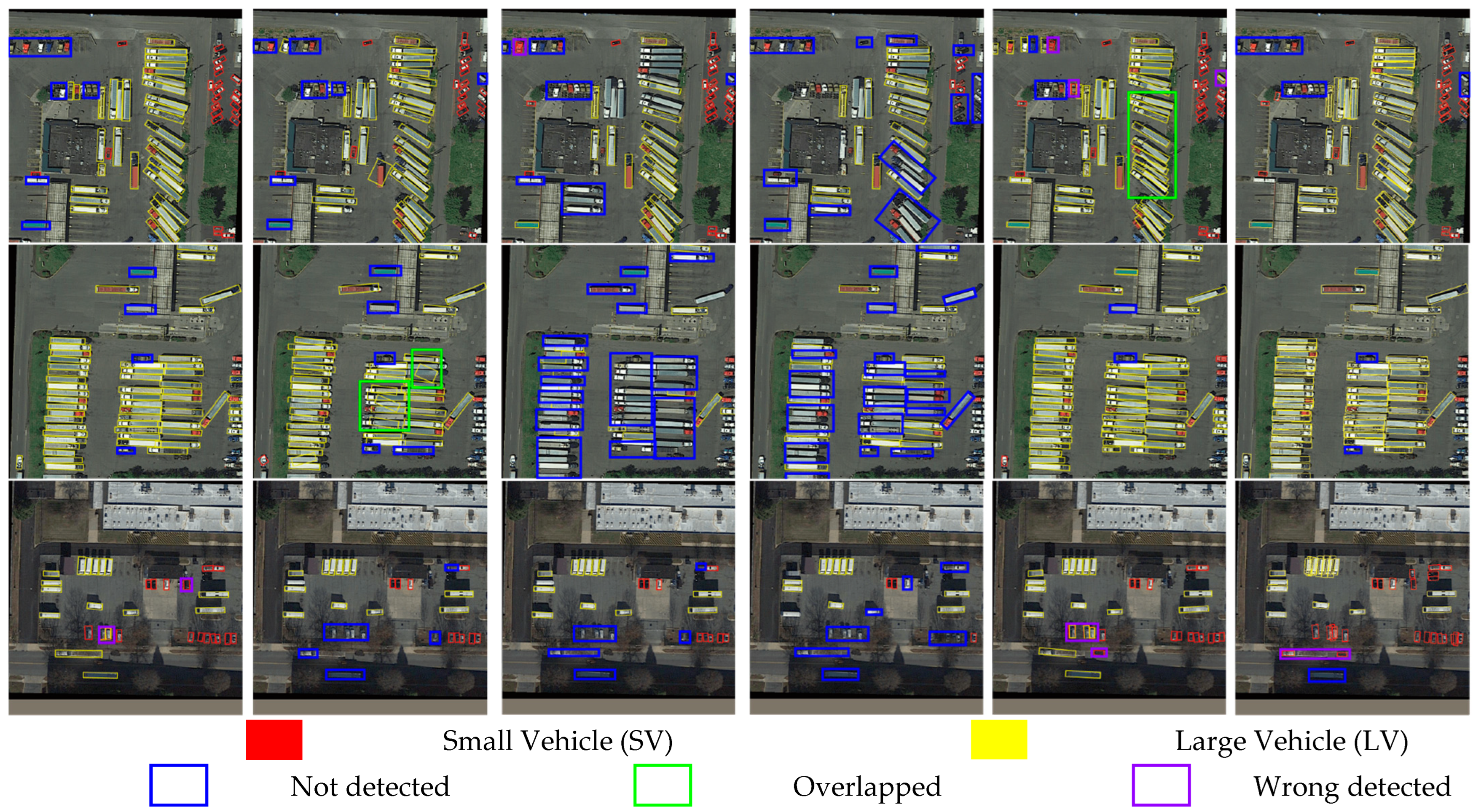
The DOTA dataset is a commonly used large remote sensing rotational telemetry detection dataset that provides a comprehensive measure of model detection performance.

Table 9. Comparison of indicators for different advanced models on DOTA dataset.

Methods	$\mathbf{A}\mathbf{P}$															$\mathbf{m}\mathbf{A}\mathbf{P}$
	PL	BD	BR	GTF	SV	LV	SH	TC	BC	ST	SBF	RA	HA	SP	HC
CFA	88.0	82.1	53.9	73.7	79.9	78.9	87.2	90.8	91.9	85.6	56.1	64.4	70.2	70.6	38.1	73.44
Rotated-FCOS	89.0	74.3	48.0	58.6	79.3	74.0	86.8	90.9	83.3	83.8	55.9	62.9	64.1	67.6	47.7	71.08
Oriented-Reppoints	88.2	78.1	51.3	73.0	79.2	76.9	87.5	90.9	83.4	84.6	64.0	64.9	66.0	69.6	48.5	73.73
ReDet	89.2	83.8	52.2	71.1	78.1	82.5	88.2	90.9	87.2	86.0	65.5	62.9	75.9	70.0	66.7	76.67
YOLOv5s-obb	89.3	84.5	51.4	60.7	80.7	84.7	88.4	90.7	85.9	87.5	59.6	65.2	74.5	81.7	66.9	76.79
Gliding vertex	89.0	77.3	47.8	68.5	74.0	74.9	85.9	90.8	84.9	84.8	53.6	64.9	64.8	69.3	57.7	72.56
RoI Transformer	89.2	84.2	51.5	72.2	78.3	77.4	87.5	90.9	86.3	85.6	63.2	66.5	68.2	71.9	60.4	75.56
RoI Transformer *	89.4	83.8	52.8	74.2	78.7	83.1	88.0	91.0	86.2	87.0	61.7	62.6	74.1	71.0	63.5	76.48
R3Det	89.4	76.9	45.8	71.5	76.9	74.6	82.4	90.8	78.1	84.0	60.1	63.7	62.1	66.1	39.2	70.77
O-RCNN *	89.5	82.8	54.2	75.2	78.6	84.9	88.1	90.9	88.1	86.6	66.9	66.7	75.4	71.6	64.0	77.56
S2Anet	88.3	79.8	46.3	71.2	77.0	73.5	79.8	90.8	82.9	82.8	55.4	62.1	61.9	69.0	51.5	71.49
Oriented-RetinaNet	89.4	80.1	39.7	69.5	77.7	61.8	77.0	90.7	82.4	80.7	56.5	64.8	55.3	64.8	43.1	68.91
Faster R-CNN-O	89.3	82.7	49.0	69.8	74.0	72.5	85.4	90.9	83.9	84.6	54.7	65.2	65.3	68.8	57.6	72.92
R-YOLO [53]	90.2	84.5	54.3	68.5	78.9	87.0	89.3	90.8	74.3	89.1	66.8	67.8	74.5	74.2	65.1	77.01
Oriented-YOLOv5 [54]	93.4	83.4	57.9	68.5	78.0	87.0	90.1	94.1	82.2	80.6	60.6	68.8	76.9	67.2	68.6	76.17
ML-Det (ours)	89.4	85.1	51.4	72.5	80.5	85.6	85.7	90.5	88.3	85.6	62.0	65.0	76.8	83.2	64.5	77.74

The optimal indicators have been bolded and reddened. For the unlabeled models in the upper right corner, the backbone and neck are taken as R50 + FPN, while for those marked with “*” in the upper right corner, the backbone and neck are set as Swin-tiny + FPN.

shows 16 different detection methods, including our proposed ML-Det, which covers the classical O-RCNN and Faster R-CNN-O algorithms, as well as other novel rotating target detection algorithms, including Oriented-Reppoints, RoI Transformer, and S²Anet. The model proposed in this paper achieves a precision of 77.74%, leading all other algorithms for the mAP test result of single-scale training, while the index is optimal in five types of target detection, namely, baseball diamonds (BD), large vehicles (LV), basketball courts (BC) and swimming pools (SP), which achieve Aps of 85.1%, 85.6%, 88.3%, and 83.2%, respectively. As shown in the visualization results in Figure 16, we can see that both large and small vehicles can learn multiple features of different targets. We also compared ten detection methods, such as ReDet, Oriented-RetinaNet, S²Anet, Gliding vertex and the ML-Det algorithm proposed in this paper, across three difficult detection scenarios. In scenario ①, it can be seen that both large vehicles (LV) and small vehicles (LV) exhibit multi-angle and dense distribution features, and a row of small vehicles in the upper left of the image is actually the front end of large vehicles. Oriented-RetinaNet, S²Anet, Faster R-CNN-O, Gliding vertex and RoI Transformer were able to correctly detect three large vehicles. Models such as ML-Det, O-RCNN*, R³Det, and Oriented-Reppoints have poorer detection results, and most of them failed to detect or detected incorrectly. In the lower right, RoI Transformer and Faster R-CNN-O have obvious detection box overlapping problems when the angle of large vehicles is gradually incremented, Oriented-RetinaNet cannot even cope with the scenario of dense rows of large vehicles, and ML-Det shows no box overlapping. In scenario ②, only some vehicle targets are cropped in the bottom right and are not used as evaluation criteria. ML-Det, S²Anet, and Faster R-CNN-O show good detection results, and Oriented-RetinaNet, Oriented-Reppoints, and FCOS miss many vehicle targets during the detection of large vehicles that are closely spaced in double rows. R³Det is prone to produce overlapping detection frames, and these can be directly overlapped into the original normal detection boxes. In scenario ③, tree shading decreases the local contrast of the picture, and R³Det, Oriented-Reppoints, Oriented-RetinaNet and FCOS are completely unable to detect the vehicle target, while S²Anet, Gliding vertex, and RoI Transformer have strong anti-jamming abilities and can detect the targets accurately. ML-Det can detect part of the vehicle targets.

4.5.4. Detection Performance Analysis

FPS is the real-time data metric measured with 4090 GPU at full load, while GFLOPS and Params are always used to verify how lightweight the model is. ML-Det is ahead of many lightweight indicators, with only 20.10 GFLOPS, 7.91 M and 78.8 FPS. The metrics in the detection performance of the different models are listed in

Table 10. Detection performance of the different models on MiVehicle datasets.

Methods	GFLOPS	FPS	Params (M)
CFA	117.94	29.9	36.60
Gliding vertex	120.73	29.3	41.13
Oriented-Reppoints	117.94	10.7	36.60
ReDet	33.80	16.2	31.57
S2ANet	119.36	26.7	38.55
O-RCNN	120.81	22.3	41.13
RoI Transformer	121.77	19.0	55.06
Faster R-CNN-O	120.73	23.5	41.13
RTMDet-S	22.79	52.21	8.86
Yolov5s-obb	17.70	81.3	7.78
ML-Det	20.10	78.8	7.91

.

5. Discussion

ML-Det has powerful feature extraction power for different datasets, not only in terms of accuracy but also in terms of how lightweight they are. However, there remains room for improvement in the model. For example, when dealing with dense rows of vehicles, the wrong detection rate of the model will rise dramatically, and it has a high probability to produce an overlap between the detection boxes. In the actual detection process, trucks are often misclassified as vans. Meanwhile, it is an undeniable fact that the model struggles with recognizing scenes with darker colors. In the DOTA dataset, when the shadow in the background of the region is concentrated, there are many unselected targets.

In the future, we will further improve our model in terms of these following aspects: ① Currently, ML-Det can only detect objects with rich features and clear contours, which are noticeable to the naked eye. We will try to detect small targets with only a few dozens of pixels, testing the applicability of the model. ② The weight of the model should be further reduced, so as to make it suitable for autonomous navigation and other occasions with higher lightweight requirements. ③ We will strive to further improve the accuracy of the model under complex backgrounds, so that the model can detect objects more efficiently in these challenging scenes. ④ We have observed that the zero-shot approach [55], which transfers learned features and patterns from the training data to unseen classes, enables the classification of objects that the model has not encountered before. In the future, we plan to explore the use of zero-shot methods to further enhance the model’s generalization capability.

6. Conclusions

In this paper, we have proposed an advanced vehicle target detection algorithm, ML-Det. We have improved the detection precision of the model with innovations and, to a great extent, have ensured that the model is lightweight. First, we propose a new neck structure, TCFPN, which enables the model to fully fuse three different levels of feature maps, significantly improving model precision, making it an efficient and lightweight neck structure. The model achieved a precision of 77.87%. Second, based on involution convolution, we proposed an efficient LKC–INVO convolution by innovatively using a large kernel multi-branch coupling structure. Here, we couple three different convolutions of 5 × 1, 5 × 5, and 5 × 1, we broaden the range of receptive fields of the model, and enhance the extraction ability of the model to extract the high-level information. Moreover, LKC–INVO convolution captured the special-agnostic and channel-specific characteristics of involution and was able to reduce the number of Params in the model. We then proposed a novel module C2F_ContextGuided modular convolution module with global context perception by combining C2F and ContextGuided, which can well utilize the information interaction of context to improve the model’s precision. In addition, we developed a new assemble–disperse attention mechanism. By aggregating local feature information, we finally tested our model by using the MiVehicle dataset with a more balanced sample distribution as well as the public UCAS_AOD and DOTA datasets. The mAP on the MiVehicle dataset reached 70.44% and 79.12% on the visible and infrared images, respectively. The model ran at 78.8 FPS on a 4090 GPU, which meets the real-time detection requirements. The Params of the model are only 7.91 M. The mAP on the UCAS_AOD dataset reached 95.25%. The mAP on DOTA dataset under the single-scale training approach reached 77.74%.

References

1. Tarolli, P.; Mudd, S.M. Remote Sensing of Geomorphology; Elsevier: Amsterdam, The Netherlands, 2020; Volume 23, ISBN 0-444-64177-7. [Google Scholar]
2. Yin, L.; Wang, L.; Li, J.; Lu, S.; Tian, J.; Yin, Z.; Liu, S.; Zheng, W. YOLOV4_CSPBi: Enhanced Land Target Detection Model. Land 2023, 12, 1813. [Google Scholar] [CrossRef]
3. Zhang, Y.; Guo, Z.; Wu, J.; Tian, Y.; Tang, H.; Guo, X. Real-Time Vehicle Detection Based on Improved Yolo V5. Sustainability 2022, 14, 12274. [Google Scholar] [CrossRef]
4. Carrasco, D.P.; Rashwan, H.A.; García, M.Á.; Puig, D. T-YOLO: Tiny Vehicle Detection Based on YOLO and Multi-Scale Convolutional Neural Networks. IEEE Access 2021, 11, 22430–22440. [Google Scholar] [CrossRef]
5. Xia, G.-S.; Bai, X.; Ding, J.; Zhu, Z.; Belongie, S.; Luo, J.; Datcu, M.; Pelillo, M.; Zhang, L. DOTA: A Large-Scale Dataset for Object Detection in Aerial Images. In Proceedings of the IEEE Conference on Computer Vision and Pattern Recognition, Salt Lake City, UT, USA, 18–23 June 2018; pp. 3974–3983. [Google Scholar]
6. Li, K.; Wan, G.; Cheng, G.; Meng, L.; Han, J. Object Detection in Optical Remote Sensing Images: A Survey and a New Benchmark. ISPRS J. Photogramm. Remote Sens. 2020, 159, 296–307. [Google Scholar] [CrossRef]
7. Sun, Y.; Cao, B.; Zhu, P.; Hu, Q. Drone-Based RGB-Infrared Cross-Modality Vehicle Detection via Uncertainty-Aware Learning. IEEE Trans. Circuits Syst. Video Technol. 2022, 32, 6700–6713. [Google Scholar] [CrossRef]
8. Zhu, H.; Chen, X.; Dai, W.; Fu, K.; Ye, Q.; Jiao, J. Orientation Robust Object Detection in Aerial Images Using Deep Convolutional Neural Network. In Proceedings of the 2015 IEEE International Conference on Image Processing (ICIP), Quebec City, QC, Canada, 27–30 September 2015; pp. 3735–3739. [Google Scholar]
9. Lin, T.-Y.; Dollár, P.; Girshick, R.; He, K.; Hariharan, B.; Belongie, S. Feature Pyramid Networks for Object Detection. In Proceedings of the IEEE Conference on Computer Vision and Pattern Recognition, Honolulu, HI, USA, 21–26 July 2017; pp. 2117–2125. [Google Scholar]
10. Liu, S.; Qi, L.; Qin, H.; Shi, J.; Jia, J. Path Aggregation Network for Instance Segmentation. In Proceedings of the IEEE Conference on Computer Vision and Pattern Recognition, Salt Lake City, UT, USA, 18–23 June 2018; pp. 8759–8768. [Google Scholar]
11. Ghiasi, G.; Lin, T.-Y.; Le, Q.V. Nas-Fpn: Learning Scalable Feature Pyramid Architecture for Object Detection. In Proceedings of the IEEE/CVF Conference on Computer Vision and Pattern Recognition, Long Beach, CA, USA, 15–20 June 2019; pp. 7036–7045. [Google Scholar]
12. Tan, M.; Pang, R.; Le, Q.V. Efficientdet: Scalable and Efficient Object Detection. In Proceedings of the IEEE/CVF Conference on Computer Vision and Pattern Recognition, Seattle, WA, USA, 13–19 June 2020; pp. 10781–10790. [Google Scholar]
13. Chen, Y.; Zhang, C.; Chen, B.; Huang, Y.; Sun, Y.; Wang, C.; Fu, X.; Dai, Y.; Qin, F.; Peng, Y. Accurate Leukocyte Detection Based on Deformable-DETR and Multi-Level Feature Fusion for Aiding Diagnosis of Blood Diseases. Comput. Biol. Med. 2024, 170, 107917. [Google Scholar] [CrossRef]
14. Hou, Q.; Zhou, D.; Feng, J. Coordinate Attention for Efficient Mobile Network Design. In Proceedings of the IEEE/CVF Conference on Computer Vision and Pattern Recognition, Nashville, TN, USA, 20–25 June 2021; pp. 13713–13722. [Google Scholar]
15. Iandola, F.N.; Han, S.; Moskewicz, M.W.; Ashraf, K.; Dally, W.J.; Keutzer, K. SqueezeNet: AlexNet-Level Accuracy with 50× Fewer Parameters and <0.5 MB Model Size. arXiv 2016, arXiv:1602.07360. [Google Scholar]
16. Howard, A.G.; Zhu, M.; Chen, B.; Kalenichenko, D.; Wang, W.; Weyand, T.; Andreetto, M.; Adam, H. Mobilenets: Efficient Convolutional Neural Networks for Mobile Vision Applications. arXiv 2017, arXiv:1704.04861. [Google Scholar]
17. Sandler, M.; Howard, A.; Zhu, M.; Zhmoginov, A.; Chen, L.-C. Mobilenetv2: Inverted Residuals and Linear Bottlenecks. In Proceedings of the IEEE Conference on Computer Vision and Pattern Recognition, Salt Lake City, UT, USA, 18–23 June 2018; pp. 4510–4520. [Google Scholar]
18. Howard, A.; Sandler, M.; Chu, G.; Chen, L.-C.; Chen, B.; Tan, M.; Wang, W.; Zhu, Y.; Pang, R.; Vasudevan, V. Searching for Mobilenetv3. In Proceedings of the IEEE/CVF International Conference on Computer Vision, Seoul, Republic of Korea, 27 October–2 November 2019; pp. 1314–1324. [Google Scholar]
19. Zhang, X.; Zhou, X.; Lin, M.; Sun, J. Shufflenet: An Extremely Efficient Convolutional Neural Network for Mobile Devices. In Proceedings of the IEEE Conference on Computer Vision and Pattern Recognition, Salt Lake City, UT, USA, 18–23 June 2018; pp. 6848–6856. [Google Scholar]
20. Ma, N.; Zhang, X.; Zheng, H.-T.; Sun, J. Shufflenet v2: Practical Guidelines for Efficient Cnn Architecture Design. In Proceedings of the European Conference on Computer Vision (ECCV), Munich, Germany, 8–14 September 2018; pp. 116–131. [Google Scholar]
21. Koonce, B.; Koonce, B. EfficientNet. In Convolutional Neural Networks with Swift for Tensorflow: Image Recognition and Dataset Categorization; Apress: Berkeley, CA, USA, 2021; pp. 109–123. [Google Scholar] [CrossRef]
22. Han, K.; Wang, Y.; Tian, Q.; Guo, J.; Xu, C.; Xu, C. Ghostnet: More Features from Cheap Operations. In Proceedings of the IEEE/CVF Conference on Computer Vision and Pattern Recognition, Seattle, WA, USA, 13–19 June 2020; pp. 1580–1589. [Google Scholar]
23. Ding, X.; Zhang, X.; Ma, N.; Han, J.; Ding, G.; Sun, J. Repvgg: Making Vgg-Style Convnets Great Again. In Proceedings of the IEEE/CVF Conference on Computer Vision and Pattern Recognition, Nashville, TN, USA, 20–25 June 2021; pp. 13733–13742. [Google Scholar]
24. Yu, C.; Jiang, X.; Wu, F.; Fu, Y.; Zhang, Y.; Li, X.; Fu, T.; Pei, J. Research on Vehicle Detection in Infrared Aerial Images in Complex Urban and Road Backgrounds. Electronics 2024, 13, 319. [Google Scholar] [CrossRef]
25. Ammour, N.; Alhichri, H.; Bazi, Y.; Benjdira, B.; Alajlan, N.; Zuair, M. Deep Learning Approach for Car Detection in UAV Imagery. Remote Sens. 2017, 9, 312. [Google Scholar] [CrossRef]
26. Ghasemi Darehnaei, Z.; Rastegar Fatemi, S.M.J.; Mirhassani, S.M.; Fouladian, M. Ensemble Deep Learning Using Faster R-Cnn and Genetic Algorithm for Vehicle Detection in Uav Images. IETE J. Res. 2023, 69, 5102–5111. [Google Scholar] [CrossRef]
27. Ma, B.; Liu, Z.; Jiang, F.; Yan, Y.; Yuan, J.; Bu, S. Vehicle Detection in Aerial Images Using Rotation-Invariant Cascaded Forest. IEEE Access 2019, 7, 59613–59623. [Google Scholar] [CrossRef]
28. Li, Q.; Mou, L.; Xu, Q.; Zhang, Y.; Zhu, X.X. R3-Net: A Deep Network for Multi-Oriented Vehicle Detection in Aerial Images and Videos. arXiv 2018, arXiv:1808.05560. [Google Scholar]
29. Li, X.; Men, F.; Lv, S.; Jiang, X.; Pan, M.; Ma, Q.; Yu, H. Vehicle Detection in Very-High-Resolution Remote Sensing Images Based on an Anchor-Free Detection Model with a More Precise Foveal Area. ISPRS Int. J. Geo-Inf. 2021, 10, 549. [Google Scholar] [CrossRef]
30. Hu, J.; Shen, L.; Sun, G. Squeeze-and-Excitation Networks. In Proceedings of the IEEE Conference on Computer Vision and Pattern Recognition, Salt Lake City, UT, USA, 18–23 June 2018; pp. 7132–7141. [Google Scholar]
31. Lee, Y.; Park, J. Centermask: Real-Time Anchor-Free Instance Segmentation. In Proceedings of the IEEE/CVF Conference on Computer Vision and Pattern Recognition, Seattle, WA, USA, 13–19 June 2020; pp. 13906–13915. [Google Scholar]
32. Wang, Q.; Wu, B.; Zhu, P.; Li, P.; Zuo, W.; Hu, Q. ECA-Net: Efficient Channel Attention for Deep Convolutional Neural Networks. In Proceedings of the IEEE/CVF Conference on Computer Vision and Pattern Recognition, Seattle, WA, USA, 13–19 June 2020; pp. 11534–11542. [Google Scholar]
33. Woo, S.; Park, J.; Lee, J.-Y.; Kweon, I.S. Cbam: Convolutional Block Attention Module. In Proceedings of the European Conference on Computer Vision (ECCV), Munich, Germany, 8–14 September 2018; pp. 3–19. [Google Scholar]
34. Chen, Y.; Kalantidis, Y.; Li, J.; Yan, S.; Feng, J. A^ 2-Nets: Double Attention Networks. arXiv 2018, arXiv:1810.11579. [Google Scholar]
35. Zhang Yu-Bin Yang, Q.-L. SA-Net: Shuffle Attention for Deep Convolutional Neural Networks. arXiv 2021, arXiv:2102.00240. [Google Scholar]
36. Hu, J.; Shen, L.; Albanie, S.; Sun, G.; Vedaldi, A. Gather-Excite: Exploiting Feature Context in Convolutional Neural Networks. arXiv 2018, arXiv:1810.12348. [Google Scholar]
37. Liu, Y.; Shao, Z.; Teng, Y.; Hoffmann, N. NAM: Normalization-Based Attention Module. arXiv 2021, arXiv:2111.12419. [Google Scholar]
38. Yang, L.; Zhang, R.-Y.; Li, L.; Xie, X. Simam: A Simple, Parameter-Free Attention Module for Convolutional Neural Networks. In Proceedings of the International Conference on Machine Learning, PMLR, Online, 18–24 July 2021; pp. 11863–11874. [Google Scholar]
39. Cao, Y.; Xu, J.; Lin, S.; Wei, F.; Hu, H. Gcnet: Non-Local Networks Meet Squeeze-Excitation Networks and Beyond. In Proceedings of the IEEE/CVF International Conference on Computer Vision (ICCV), Seoul, Republic of Korea, 27 October–2 November 2019; pp. 1–10. [Google Scholar]
40. Li, X.; Hu, X.; Yang, J. Spatial Group-Wise Enhance: Improving Semantic Feature Learning in Convolutional Networks. arXiv 2019, arXiv:1905.09646. [Google Scholar]
41. Yang, X.; Yan, J. Arbitrary-Oriented Object Detection with Circular Smooth Label; Springer: Berlin/Heidelberg, Germany, 2020; pp. 677–694. [Google Scholar]
42. Li, D.; Hu, J.; Wang, C.; Li, X.; She, Q.; Zhu, L.; Zhang, T.; Chen, Q. Involution: Inverting the Inherence of Convolution for Visual Recognition. In Proceedings of the IEEE/CVF Conference on Computer Vision and Pattern Recognition, Nashville, TN, USA, 20–25 June 2021; pp. 12321–12330. [Google Scholar]
43. Wang, C.-Y.; Bochkovskiy, A.; Liao, H.-Y.M. YOLOv7: Trainable Bag-of-Freebies Sets New State-of-the-Art for Real-Time Object Detectors. In Proceedings of the IEEE/CVF Conference on Computer Vision and Pattern Recognition, Vancouver, BC, Canada, 17–24 June 2023; pp. 7464–7475. [Google Scholar]
44. Lee, S.; Lee, S.; Song, B.C. Cfa: Coupled-Hypersphere-Based Feature Adaptation for Target-Oriented Anomaly Localization. IEEE Access 2022, 10, 78446–78454. [Google Scholar] [CrossRef]
45. Xu, Y.; Fu, M.; Wang, Q.; Wang, Y.; Chen, K.; Xia, G.-S.; Bai, X. Gliding Vertex on the Horizontal Bounding Box for Multi-Oriented Object Detection. IEEE Trans. Pattern Anal. Mach. Intell. 2020, 43, 1452–1459. [Google Scholar] [CrossRef] [PubMed]
46. Li, W.; Chen, Y.; Hu, K.; Zhu, J. Oriented Reppoints for Aerial Object Detection. In Proceedings of the IEEE/CVF conference on computer vision and pattern recognition, New Orleans, LA, USA, 18–24 June 2022; pp. 1829–1838. [Google Scholar]
47. Han, J.; Ding, J.; Xue, N.; Xia, G.-S. Redet: A Rotation-Equivariant Detector for Aerial Object Detection. arXiv 2021, arXiv:2103.07733. [Google Scholar]
48. Han, J.; Ding, J.; Li, J.; Xia, G.-S. Align Deep Features for Oriented Object Detection. IEEE Trans. Geosci. Remote Sens. 2021, 60, 1–11. [Google Scholar] [CrossRef]
49. Jiang, Y.; Zhu, X.; Wang, X.; Yang, S.; Li, W.; Wang, H.; Fu, P.; Luo, Z. R2CNN: Rotational Region CNN for Orientation Robust Scene Text Detection. arXiv 2017, arXiv:1706.09579. [Google Scholar]
50. Ding, J.; Xue, N.; Long, Y.; Xia, G.-S.; Lu, Q. Learning RoI Transformer for Oriented Object Detection in Aerial Images. In Proceedings of the IEEE/CVF Conference on Computer Vision and Pattern Recognition, Long Beach, CA, USA, 15–20 June 2019; pp. 2849–2858. [Google Scholar]
51. Yang, S.; Pei, Z.; Zhou, F.; Wang, G. Rotated Faster R-CNN for Oriented Object Detection in Aerial Images. In Proceedings of the 2020 3rd International Conference on Robot Systems and Applications, Chengdu, China, 14–16 June 2020; pp. 35–39. [Google Scholar]
52. Lyu, C.; Zhang, W.; Huang, H.; Zhou, Y.; Wang, Y.; Liu, Y.; Zhang, S.; Chen, K. Rtmdet: An Empirical Study of Designing Real-Time Object Detectors. arXiv 2022, arXiv:2212.07784. [Google Scholar]
53. Hou, Y.; Shi, G.; Zhao, Y.; Wang, F.; Jiang, X.; Zhuang, R.; Mei, Y.; Ma, X. R-YOLO: A YOLO-Based Method for Arbitrary-Oriented Target Detection in High-Resolution Remote Sensing Images. Sensors 2022, 22, 5716. [Google Scholar] [CrossRef]
54. Qing, H.U.; Li, R.; Pan, C.; Gao, O. Remote Sensing Image Object Detection Based on Oriented Bounding Box and Yolov5. In Proceedings of the 2022 IEEE 10th Joint International Information Technology and Artificial Intelligence Conference (ITAIC), Chongqing, China, 17–19 June 2022; Volume 10, pp. 657–661. [Google Scholar]
55. Socher, R.; Ganjoo, M.; Manning, C.D.; Ng, A. Zero-Shot Learning through Cross-Modal Transfer. Adv. Neural Inf. Process. Syst. 2013, 26, 1–7. [Google Scholar]
Figure 1. Comparison of horizontal and rotating boxes for arbitrary rotating vehicle target selection: (a) horizontal box and (b) rotating box.
Remotesensing 16 03637 g001
Figure 2. General architecture of the ML-Det model.
Remotesensing 16 03637 g002
Figure 3. The structure of the SPPX model. “*” denotes multiplication, and the following number represents the number of modules.
Remotesensing 16 03637 g003
Figure 4. Schematic diagram of LKC–INVO convolution.
Remotesensing 16 03637 g004
Figure 5. Comparison of model features before and after adding LKC–INVO convolution. (a) Before and (b) after adding LKC–INVO convolution.
Remotesensing 16 03637 g005
Figure 6. C2F_ContextGuided schematic diagram. (a) C2F_ContextGuide and (b) CG_Bottleneck Block.
Remotesensing 16 03637 g006aRemotesensing 16 03637 g006b
Figure 7. Assemble–disperse schematic diagram.
Remotesensing 16 03637 g007
Figure 8. Examples from the MiVehicle dataset.
Remotesensing 16 03637 g008
Figure 9. Comparison of the share of each vehicle in the dataset.
Remotesensing 16 03637 g009
Figure 10. Examples of vehicles in UCAS_AOD dataset.
Remotesensing 16 03637 g010
Figure 11. Examples of vehicles in the DOTA dataset.
Remotesensing 16 03637 g011
Figure 12. Comparison of the detection differences of YOLOv5s-obb (left) and ML-Det (right).
Remotesensing 16 03637 g012aRemotesensing 16 03637 g012b
Figure 13. Comparison of confusion matrices of YOLOv5s-obb (left) and ML-Det (right).
Remotesensing 16 03637 g013
Figure 14. Comparison of the detection effectiveness of five advanced target detection algorithms on different modalities of the MiVehicle dataset.
Remotesensing 16 03637 g014
Figure 15. Comparison of the detection effectiveness of five advanced target detection algorithms on UCAS_AOD dataset.
Remotesensing 16 03637 g015aRemotesensing 16 03637 g015b
Figure 16. Comparison of detection effectiveness of various advanced target detection algorithms in DOTA dataset.
Remotesensing 16 03637 g016aRemotesensing 16 03637 g016b