Article

Evaluation of the Operational Global Ocean Wave Forecasting System of China

1
College of Environmental Science and Engineering, Ocean University of China, Qingdao 266100, China
2
National Marine Environmental Forecasting Center, Beijing 100081, China
3
Key Laboratory of Marine Hazards Forecasting, National Marine Environmental Forecasting Center, Ministry of Natural Resources, Beijing 100081, China
4
Key Laboratory of Ministry of Education for Coastal Disaster and Protection, Hohai University, Nanjing 210098, China
5
School of Artificial Intelligence, Sun Yat-Sen University, Zhuhai 519000, China
*
Author to whom correspondence should be addressed.
Remote Sens. 2024, 16(18), 3535; https://doi.org/10.3390/rs16183535
Submission received: 10 August 2024 / Revised: 13 September 2024 / Accepted: 18 September 2024 / Published: 23 September 2024

Abstract

:
Based on the WAVEWATCH III wave model, China’s National Marine Environmental Forecasting Center has developed an operational global ocean wave forecasting system that covers the Arctic region. In this study, in situ buoy observations and satellite remote sensing data were used to perform a detailed evaluation of the system’s forecasting results for 2022, with a focus on China’s offshore and global ocean waters, so as to comprehensively understand the model’s forecasting performance. The study results showed the following: In China’s coastal waters, the model had a high forecasting accuracy for significant wave heights. The model tended to underestimate the significant wave heights in autumn and winter and overestimate them in spring and summer. In addition, the model slightly underestimated low (below 1 m) wave heights, while overestimating them in other ranges. In terms of spatial distribution, negative deviations and high scatter indexes were observed in the forecasting of significant wave heights in semi-enclosed sea areas such as the Bohai Sea, Yellow Sea, and Beibu Gulf, with the largest negative deviation occurring near Liaodong Bay of the Bohai Sea (−0.18 m). There was a slight positive deviation (0.01 m) in the East China Sea, while the South China Sea exhibited a more significant positive deviation (0.17 m). The model showed a trend of underestimation for the forecasting of the mean wave period in China’s coastal waters. In the global oceanic waters, the forecasting results of the model were found to have obvious positive deviations for most regions, with negative deviations mainly occurring on the east coast and in relatively closed basins. There were latitude differences in the forecasting deviations of the model: specifically, the most significant positive deviations occurred in the Southern Ocean, with smaller positive deviations toward the north, while a slight negative deviation was observed in the Arctic waters. Overall, the global wave model has high reliability and can meet the current operational forecasting needs. In the future, the accuracy and performance of ocean wave forecasting can be further improved by adjusting the parameterization scheme, replacing the wind fields with more accurate ones, adopting spherical multiple-cell grids, and data assimilation.

1. Introduction

Wave forecasting originated in the 1940s from the need for landing operations. In the following decades of research since that time, wave forecasting has been highly valued around the world, and its needs have gradually expanded from military activity support in the early stage to ocean development and construction, ocean transportation, ocean management, ocean disaster prevention and reduction, and so on. In the 21st century, economic globalization has made ocean issues important parts of national strategies. Wave forecasting continues to provide important technical support for the safeguarding of marine rights, protection of marine resources and environment, and rational development and sustainable use of marine resources. Against the backdrop of global efforts to address climate change, protect the environment, conserve energy, and reduce emissions, as an inexhaustible source of renewable and clean energy, coastal wave energy has become a way for humanity to help solve the energy crisis. In addition, the study of wave mechanisms itself will promote the research on mass, momentum, kinetic energy, heat exchange processes, and phase transition at the air–sea interface, thus helping to gain an in-depth understanding of the properties of air–sea boundaries and deepen our scientific understanding of related fields.
Considering the needs of ocean wave forecasting in various aspects such as the national economy, society, environment, and military, the ocean wave numerical forecasting model—based on the close combination of oceanography, fluid mechanics, and computational mathematics—has developed rapidly. After three generations of mainstream numerical models, the precision and accuracy of forecasting have been greatly improved. The ocean wave forecasting models can now basically meet the needs of various ocean wave forecasting and are currently the most important methods for ocean wave forecasting. The third-generation ocean wave numerical models, such as WAM [1,2], WAVEWATCH III [3,4], and SWAN [5], are widely used by many meteorological and ocean business centers, including the European Center for Medium-Range Weather Forecasts (ECMWF) [6,7,8], the National Centers for Environmental Prediction (NCEP) [9,10,11,12], Météo-France [13], Met Office [14], Indian National Center for Ocean Information Services (INCOIS) [15], and China’s National Marine Environmental Forecasting Center (NMEFC) [16,17,18]. These models have been used to achieve satisfactory results in wave forecasting operations at global, regional, and coastal scales.
Any business center involved in wave forecasting should conduct some form of quality monitoring on its products [19]. In 1995, under the coordination of the ECMWF, an international comparison project for ocean wave forecasting was established [20,21,22]. Later, the ECMWF, Met Office, the U.S. Navy’s Fleet Numerical Meteorology and Oceanography Center (FNMOC), the Meteorological Service of Canada (MSC), NCEP, and other institutions successively joined the cause to achieve the following: quantitatively evaluate the global and regional skills, advantages, and disadvantages of different wave forecasting systems; analyze the potential causes of model errors by collecting buoy observation data from different sea areas, and conducting a horizontal comparison of wave model data from different operational agencies; and identify potential areas for improvement. Moreover, business institutions in some countries have also carried out extensive validations and scientific assessments of their wave forecasting systems, thereby ensuring the reliability of wave forecasting. By evaluating two sets of wave forecasting systems of the Met Office—that is, the global GS512L4EUK and regional AMM15SL2—Valiente et al. showcased the compelling benefits of spherical multiple-cell (SMC) grids [23]. This approach bolsters computational efficiency, while also ensuring that the model’s predictive prowess remained uncompromised at both global and coastal scales. The authors also discussed how incorporating wave–current interactions and improving the resolution of wave model and wind forcing can enhance the accuracy of wave field simulations. Environment Canada’s global ocean wave forecasting system had undergone several improvements to its regional system, including increasing the horizontal and spectral resolutions of the wave model; incorporating ice field forcing; upgrading the physics package and atmospheric forcing, which addressed the long-standing issue of poor wave predictions in the Northeast Pacific; and improved wave forecasts under tropical cyclone conditions [24]. The Copernicus Marine Environment Monitoring Service (CMEMS) Mediterranean wave forecasting system (Med-waves) considered the sensitivity of Mediterranean wave dynamics to the nesting with the Atlantic, along with the influence of surface currents on wave refraction, and compensated for the underestimation of wind in this region by adjusting the dissipation function to reduce energy loss caused by whitecaps, thereby providing reliable Mediterranean wave forecasts [25]. The INCOIS conducted a comprehensive evaluation of its Indian Ocean wave forecasting system, and the model provided reliable simulations of waves during monsoon, cyclonic, and swell events. Further adjustments to the parameterization schemes within the model will refine the simulation of wind waves during non-monsoon months [26].
China’s NMEFC is an operational center that provides ocean forecasting—a basic public welfare service—to the public, sectors involved in maritime affairs, and government agencies. It first published China’s offshore wave forecasts nationwide in 1966. Global wave forecasting was an important business expansion of the NMEFC during the Eleventh and Twelfth Five-Year Plan periods. The introduction of advanced foreign wave models promoted the establishment of an operational global ocean wave forecasting system, and the forecasting range was extended to the Arctic during the Thirteenth Five-Year Plan period. This paper is the first to evaluate the NMEFC’s global ocean wave forecasts. In situ observations and satellite data were used to validate the forecast wave fields, including those in China’s coastal waters and various global oceans, to ensure their reliability in the use of NMEFC business. The validation results will provide a reference basis for model developers to further improve the model, and for wave forecasters to make subjective forecasting decisions.
The organizational structure of this paper is as follows: Section 2 provides a detailed description of the wave model, along with the data sources and methods used to evaluate the performance of the model; Section 3 analyzes the validation results; Section 4 presents the discussions; and finally, the conclusions are presented.

2. Wave Model, Data, and Method

2.1. Wave Model

The NMEFC’s global ocean wave forecasting system was constructed based on the third-generation wave forecasting model WAVEWATCH III 6.07 [27] developed by NOAA/NCEP, mainly considering physical processes such as wave generation in deep water, nonlinear four-wave interactions, and wave dissipation. Tolman and Chalikov’s source term package was used for input and dissipation physics. Discrete interaction approximation (DIA) was chosen for the nonlinear interactions scheme. A third-order (UQ) propagation scheme and the Tolman (2002) averaging technique were implemented with GSE alleviation. A nested grid was used, with an outer sea area ranging from 0°–360°, 78°S–78°N, a spatial resolution of 0.1°, periodic boundary conditions in the east–west direction, and land in the north–south direction; with the inner Arctic region ranging from 0°–360°, 60°N–87°N, and a spatial resolution of 0.1°. The calculation results of the outer global waters provide boundary conditions for high-latitude Arctic waters. In the two-dimensional spectral space of frequency and direction, the spectrum was divided into 25 frequency bands, with an initial frequency of 0.04118 Hz, and the relationship between each frequency band was fn + 1 = 1.1 × fn (n = 0, 1, …, 24). The wave direction was divided into 48 directions according to a uniform grid. The bathymetric data of the general bathymetric chart of the oceans (GEBCO) 15″ were used as the topographic data. NCEP/GFS global wind field forecasting data were adopted for forced wind fields. The forced sea ice data in the Arctic region included the concentration and thickness of sea ice, sourced from the Arctic Ice Ocean Prediction System (ArcIOPS), and the NEMO global ocean forecasting system developed by the NMEFC. Figure 1 shows the flowchart of the NMEFC’s global ocean wave forecasting system.

2.2. Data

Firstly, the model was validated using data from the China Ocean Monitoring Network for 2022, taken from about 30 hydrometeorological buoys in China’s coastal waters. The buoy observations were made at an interval of one hour, and the observation elements included wind speed (Ws), wind direction, atmospheric pressure, air temperature, water temperature, relative humidity, mean wave height, mean wave period (Tm), mean wave direction, one-tenth wave height, one-tenth wave period, significant wave height (Hs), significant wave period, maximum wave height, maximum wave period, and so on. The position accuracy of the buoys was 0.01′, the observation accuracy of the Hs was 0.1 m, and the observation accuracy of the wave period was 0.1 s. Prior to use, quality control of buoy observations was carried out using the method proposed by Bidlot et al. [19] to eliminate outliers.
Validation of global ocean waters was conducted using buoy data from the U.S. National Data Buoy Center (NDBC). Jason-3 satellite altimeter’s along-track Hs data were used for additional spatial validation to improve the assessment of the global ocean. Jason-3 was the successor satellite altimeter of Jason-2, and adopted the same track design, with a track height of 1336 km, inclination angle of 66°, and track revisit period of 10 days. The task of the Jason-3 altimeter was to provide continuous satellite altimetry data with the same accuracy and spatial coverage, following the TOPEX/Poseidon, Jason-1, and Jason-2 altimeters. Yang et al. [28] evaluated Hs retrievals from the Jason-3 altimeter using NDBC buoy data. Jason-3’s Hs data were consistent with the NDBC buoy data, with a deviation (Bias) of 0.05 m, root mean square error (RMSE) of 0.23 m, scatter index (SI) of 13%, and correlation coefficient (Corr) of 0.98.
For high-latitude Arctic waters, integrated satellite data products from the Copernicus Marine Environment Monitoring Service (CMEMS) were used to evaluate the model prediction performance. These data were based on the near-real-time mono-mission satellite along-track significant wave height. Only valid data were included, based on rigorous editing combining various criteria such as quality flags (surface flag, presence of ice) and thresholds on parameter values. Such thresholds were applied on parameters linked to Hs determination from retracking (such as Hs, sigma0, range, and off nadir angle). All the missions were homogenized with respect to a reference mission (Jason-3 until April 2022, Sentinel-6A afterwards) and calibrated on in situ buoy measurements. Finally, an along-track filter was applied to reduce the measurement noise. This product was processed by the WAVE-TAC multi-mission altimeter data processing system. It served, in near-real time, the main operational oceanography and climate forecasting centers in Europe, as well as worldwide ones. It processed operational data (OGDR and NRT, produced in near-real time) from the following altimeter missions: Sentinel-6A, Jason-3, Sentinel-3A, Sentinel-3B, Cryosat-2, SARAL/AltiKa, CFOSAT; and interim data (IGDR, delay of 1 to 2 days) from the HY-2B mission. Some studies [28,29,30] have confirmed that these altimeter missions can provide high-quality Hs data, and were widely used in model evaluation, data assimilation, and wave climatology construction [31]. The integrated satellite data products’ quality information document (https://catalogue.marine.copernicus.eu/documents/QUID/CMEMS-WAV-QUID-014-001.pdf, last access: 1 August 2024) showed with the absolute calibration, the altimetry measurements accurately reproduced in situ measurements with a correlation of 0.98–0.99.

2.3. Method

To evaluate the model’s forecasting performance, satellite altimeters and buoy observation data were used to verify the operational global ocean wave forecasting results of the WAVEWATCH III model, and statistics were made once a month. During the verification process, for simplicity, results with a forecast time of 0–24 h were included into a statistical group for error analysis. The meanings of the 24–48 h and 48–72 h forecasts were similar. The items of the test statistics were Bias, mean absolute error (MAE), RMSE, relative error (RE), Corr, and SI, which were, respectively, defined by the following formulas:
B i a s = 1 N i = 1 N ( P i O i )
M A E = 1 N i = 1 N ( P i O i )
R M S E = 1 N i = 1 N ( P i O i ) 2
R E = 1 N i = 1 N P i O i O i
C o r r = i = 1 N ( P i P ¯ ) ( O i O ¯ ) [ i = 1 N ( P i P ¯ ) 2 i = 1 N ( O i O ¯ ) 2 ] 1 2
S I = 1 N i = 1 N P i P ¯ O i O ¯ 2 O ¯
where Pi was the forecast value, Oi was the observed value, and N was the number of samples. When calculating RE, only Hs above 1 m were counted, while when calculating the other five statistical items, all Hs were counted.
In the statistical process, temporal and spatial registration were first performed. With the data 0.5 h before and after the hour of satellite as the data for that hour, the forecast field at that time during the 0–24 h forecast period was read. According to the latitude and longitude coordinates of the satellite data, the forecast data were bilinearly interpolated to that point as a pair of observation–forecast verification data. All the forecast verification data within a month were used as a basic statistical dataset. Similarly, test datasets such as 24–48 h forecasts and 48–72 h forecasts could be formed. For each dataset, the forecasting performance of the model was quantitatively evaluated using the aforementioned statistical methods.

3. Results

This section presents an analysis of the operational forecasts for 2022. The validations of the Hs and Tm were conducted using Chinese offshore buoy data, and the spatial validations in global ocean waters were carried out using the along-track Hs data of the Jason-3 satellite altimeter. For high-latitude Arctic waters, due to the limited amount of data from a single satellite, the fusion satellite Hs data from the CMEMS were used to evaluate the model’s forecasting performance.

3.1. Evaluation of Forecasting Performance in China’s Offshore Areas

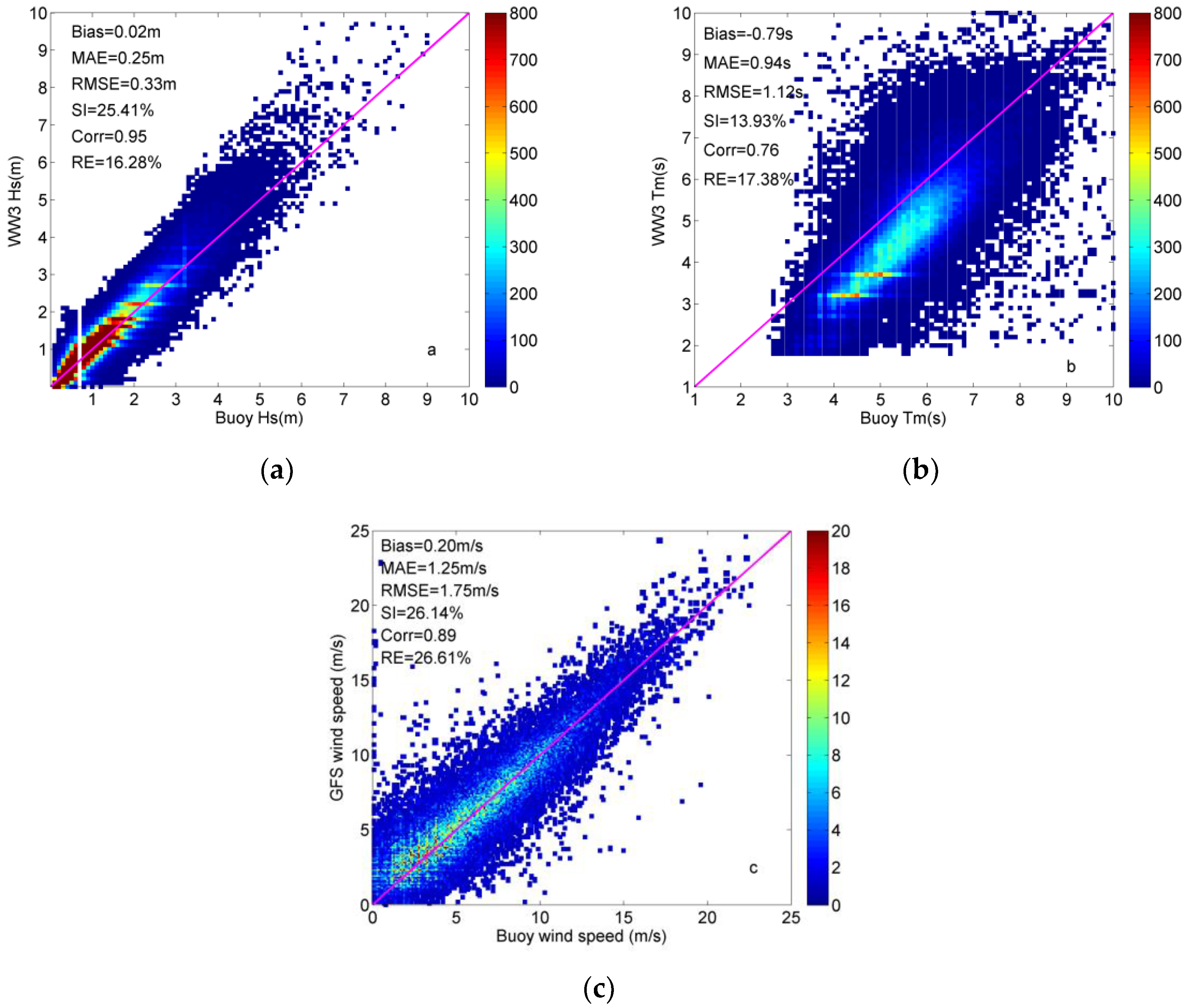
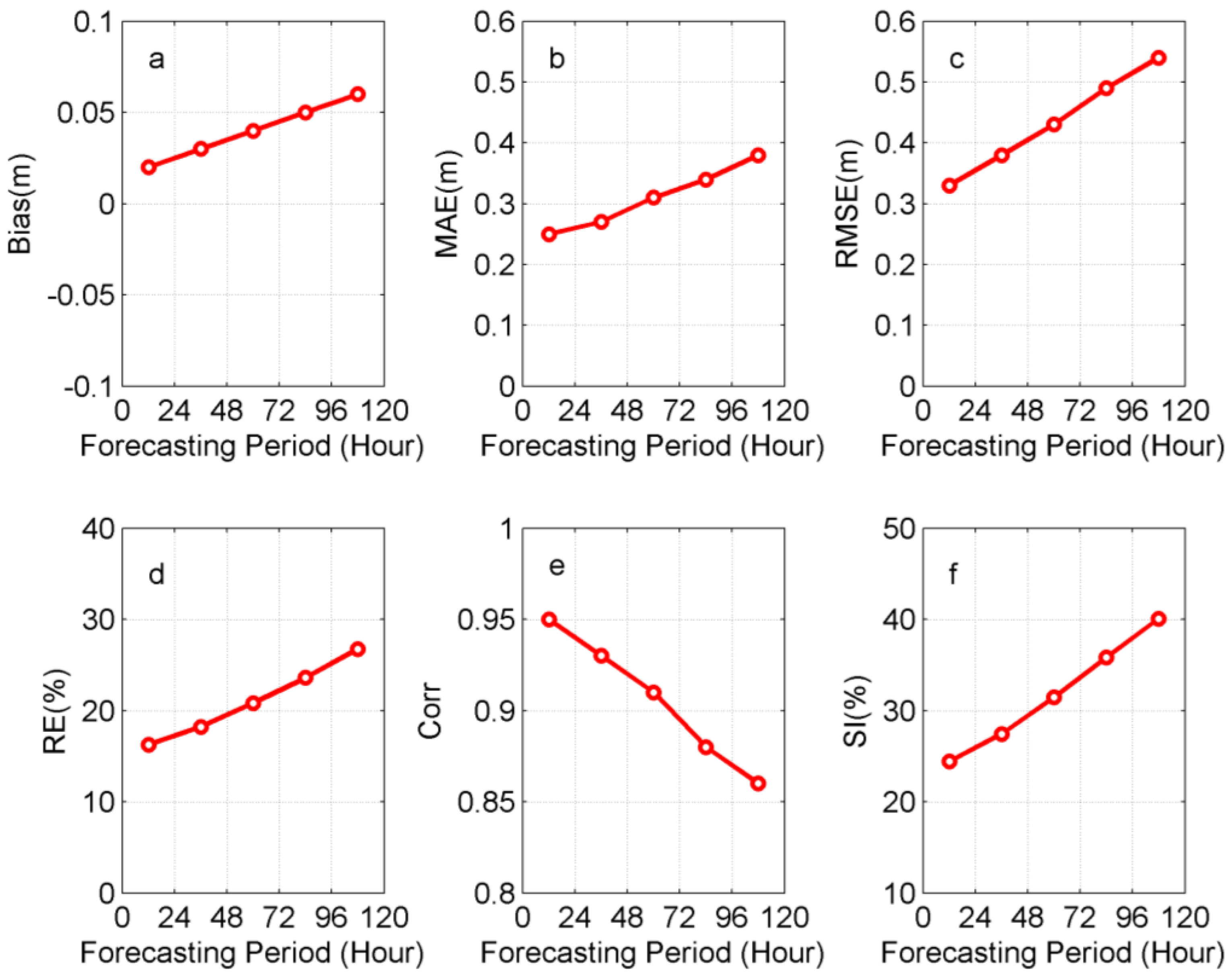
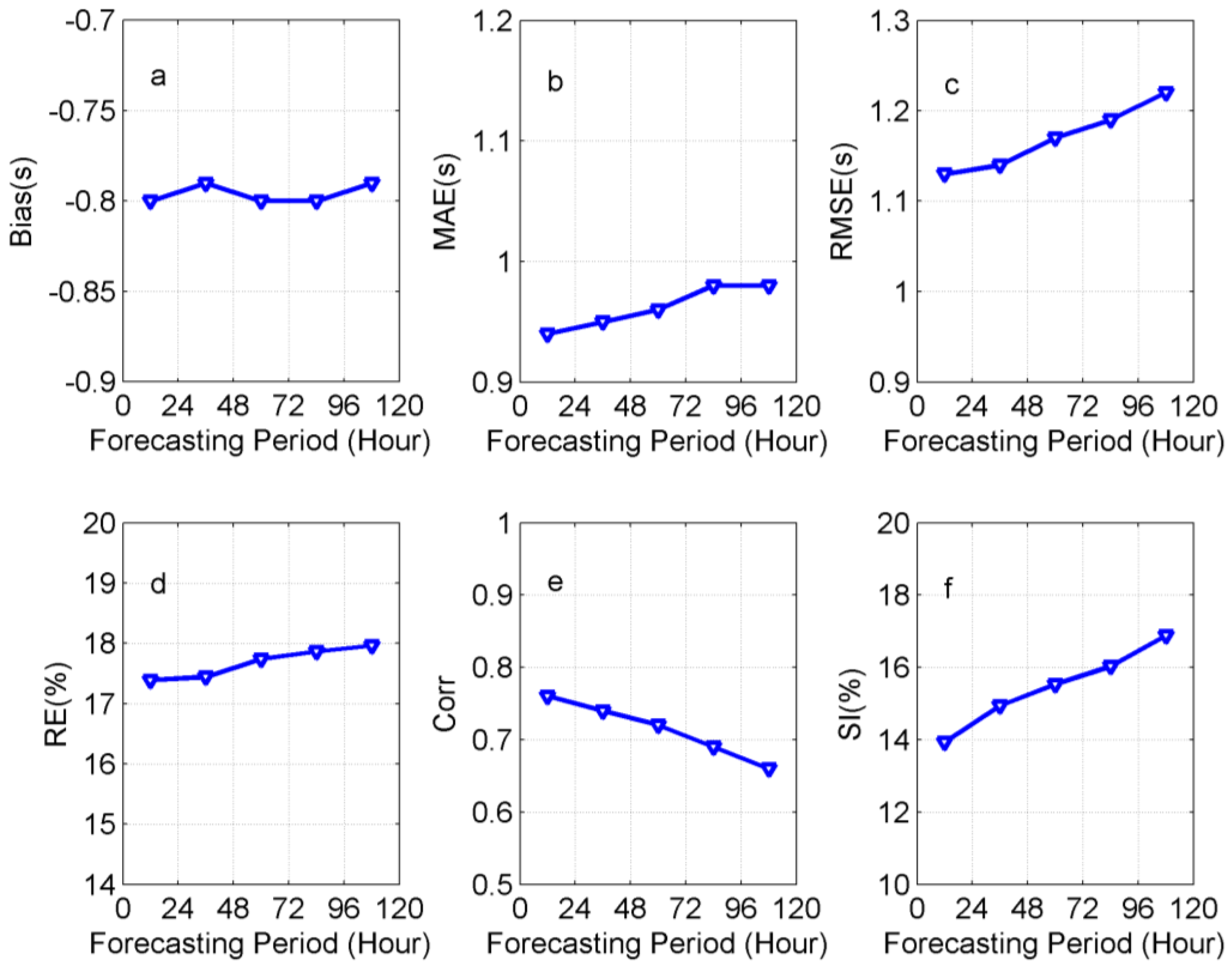
The forecasting results were tested using 29 offshore buoys in 2022, with the testing elements including the Hs, Tm, and 10 m Ws of the wind forcing field. Figure 2 shows the scatter plots of the 0–24 h forecast Hs, Tm, and Ws tests, and the values of each statistical item are also marked in the graphs. The accuracy of the Hs and Ws forecasting was relatively high, with a Bias of 0.02 m, RMSE of about 0.3 m, RE of about 16%, and Corr of 0.95 for the 0–24 h Hs forecasting. According to the scatter distribution in Figure 2b, the model tended to underestimate the Tm. Figure 3 shows that as the prediction period increased, the accuracy of the Hs forecasting decreased. The 5-day forecasting deviations were 0.02~0.06 m, MAE values less than 0.38 m, RMSE values within 0.54 m, RE values 16~26%, Corr values greater than 0.85, and SI values less than 40%. Compared with the Hs, the accuracy of the Tm forecasting during the 5-day forecast period showed a smaller decrease over time (note that the vertical coordinate ranges in Figure 4 were smaller than those in Figure 3). Especially for the SI, during the 5-day forecast period, the SI values of the Tm forecasts decreased by 3%, and those of the Hs forecasts decreased by 15%.
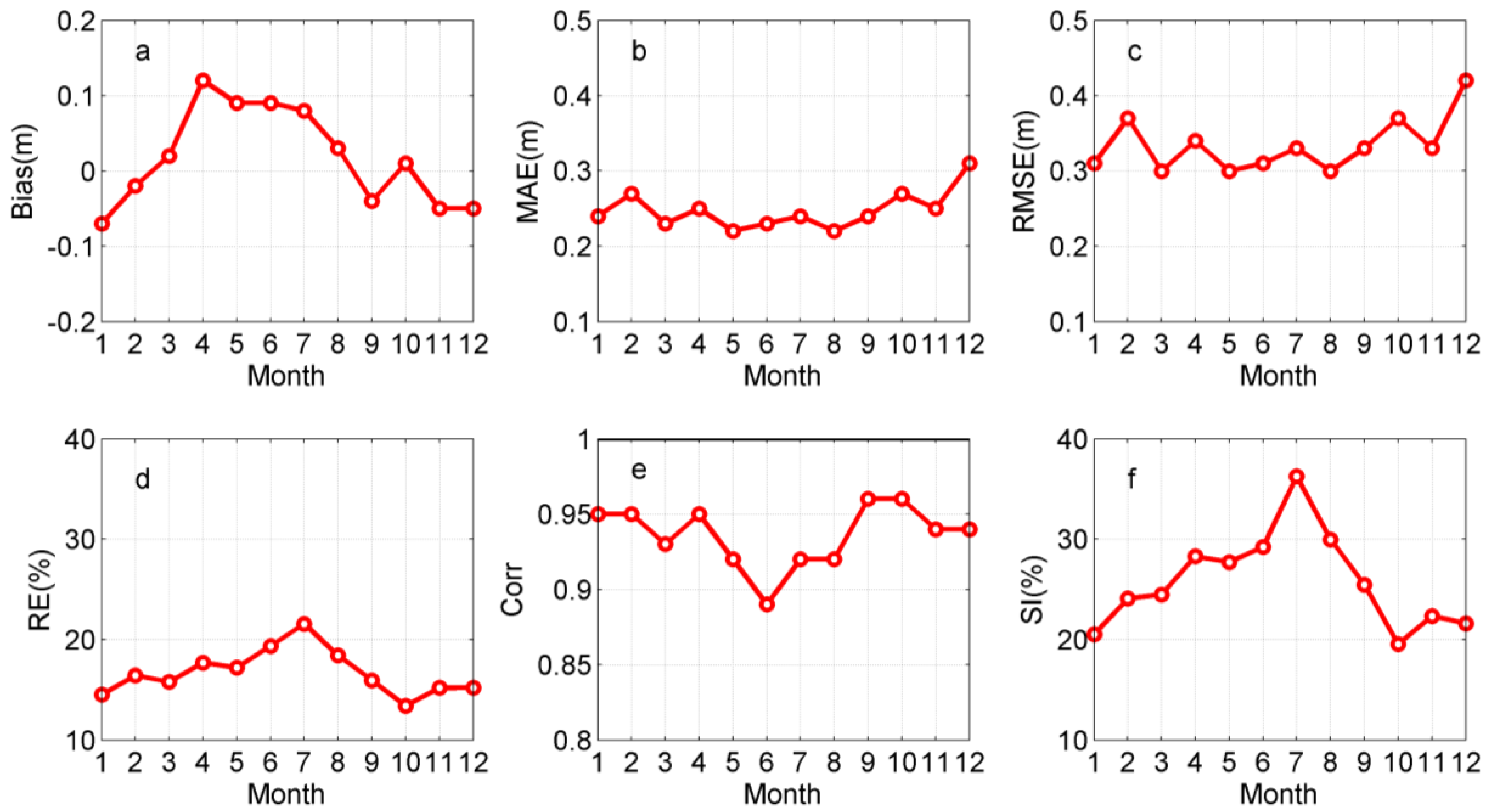
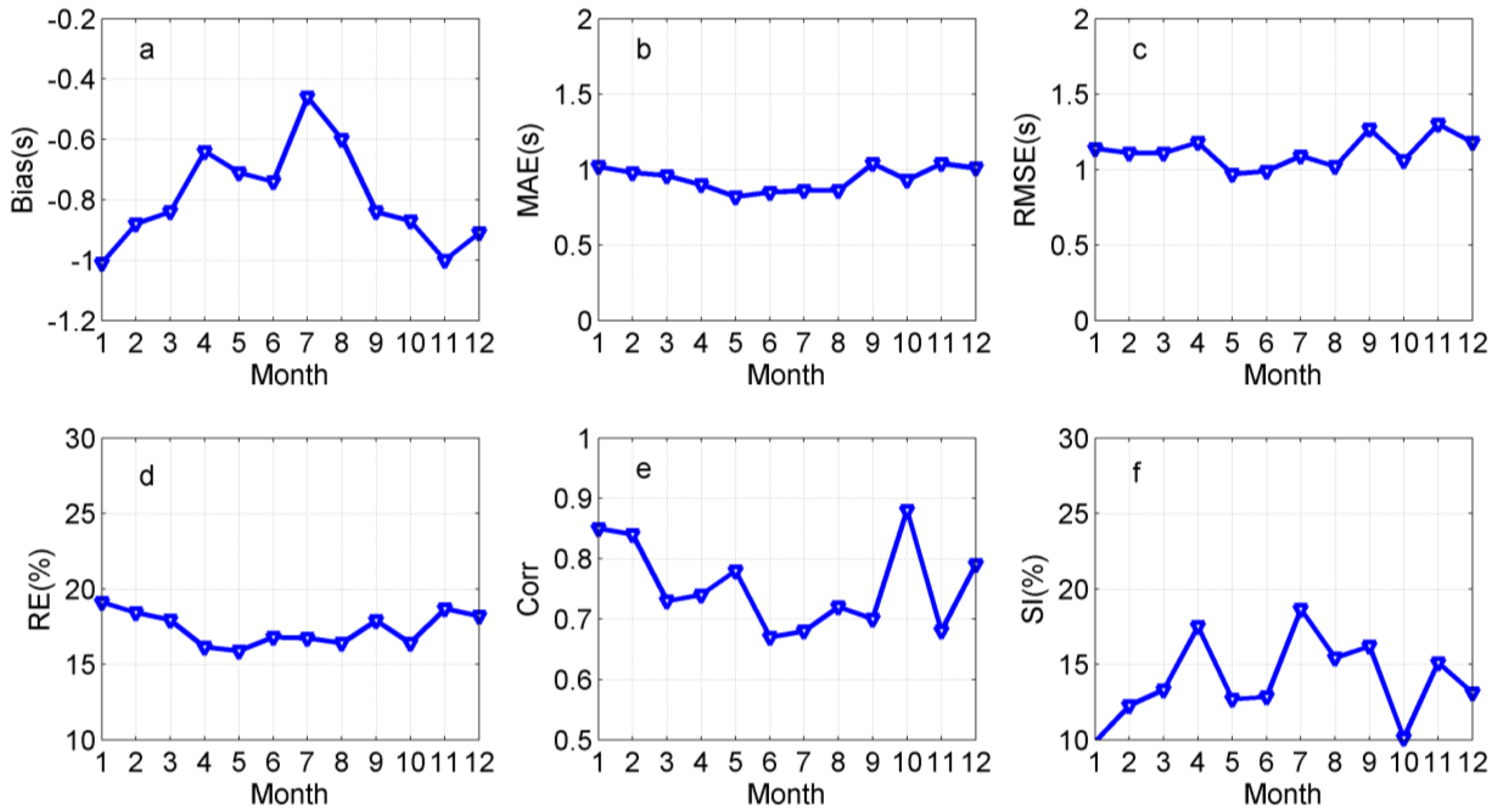
Figure 5 and Figure 6, respectively, show the error distributions of the monthly Hs and Tm forecasts. Table 1 and Table 2, respectively, provide statistics on the error parameters of the Hs and Tm forecasts for each season, to shed light on the model’s forecasting performance in different months and seasons. For the Hs forecasting, the forecast results of the model were relatively underestimated in autumn and winter and showed a positive Bias in spring and summer. This was consistent with the seasonal error characteristics exhibited by the wind forcing field. The error of wave forecasting was closely related to wind forcing. The GFS forecast wind field tested by the World Meteorological Organization (WMO) in 2022 also exhibited a slight negative Bias in the northwestern Pacific Ocean during winter, and positive Bias during summer [32]. The MAE and RMSE of the Hs forecasts in autumn and winter were greater than those in spring and summer. However, in autumn and winter, China’s offshore areas were affected by cold air from Siberia and Mongolia, with a higher wind strength and a greater average Hs than in spring and summer. The Corr, RE, and SI of the Hs forecasts in autumn and winter were more accurate than those in spring and summer. The SI of the Hs forecasts was the highest in summer (31.52%) and lowest in winter (21.75%), which was consistent with the performance of the forced wind field forecasting. The forced wind field forecasting also exhibited error characteristics, with a lower SI in winter (20.17%) and higher SI (36.49%) in summer. In addition, for the big wave events caused by cold air in autumn and winter, due to the relatively long cycle of weather system changes and large spatial scale, the model achieved a good simulation effect on cold air waves (with lower SI and higher Corr). In spring and summer, China’s offshore areas were affected by typhoons or temperate cyclones, and the model was relatively poor at simulating the big wave events caused by the rapidly changing weather system (with higher SI and lower Corr). The model also showed obvious seasonal characteristics in the Tm forecasting error. The underestimations of the Tm forecasts by the model in autumn and winter were more pronounced than those in spring and summer, and the Corr and SI of the Tm forecasts in autumn and winter were, overall, superior to those in spring and summer.
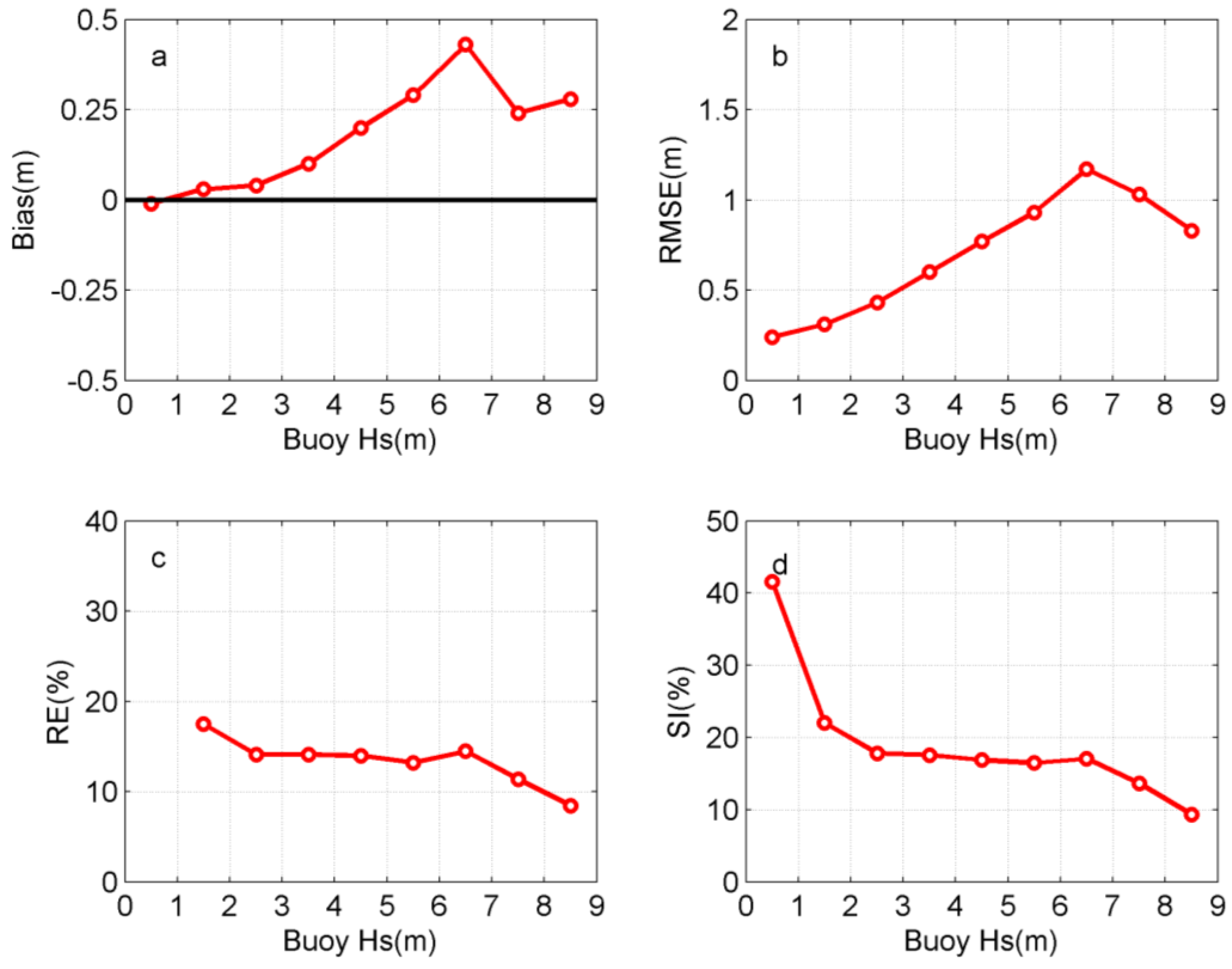
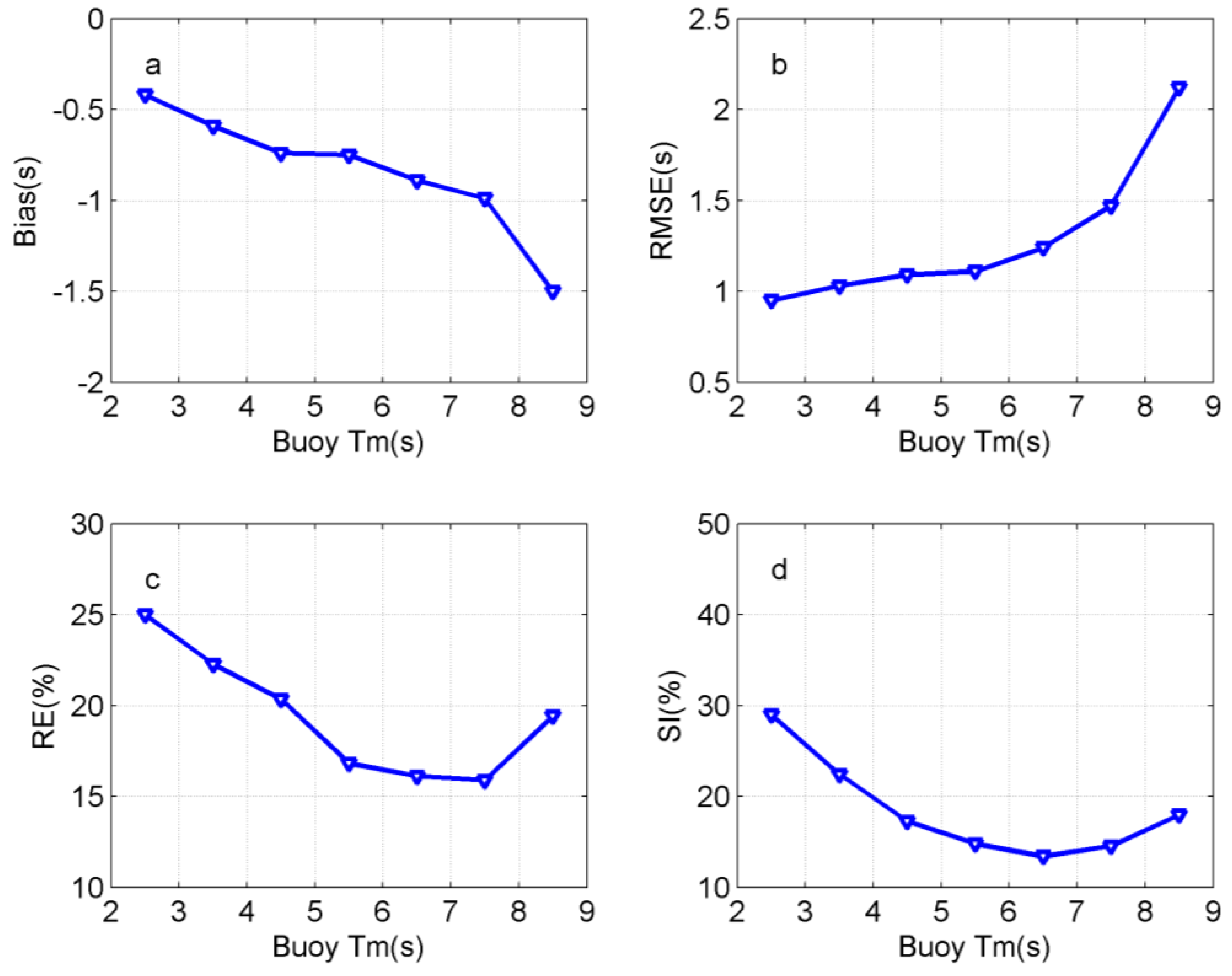
Next, the forecasting performance of the model within different Hs and Tm ranges was analyzed, taking the 0–24 h forecasts as an example (Figure 7 and Figure 8). From Figure 7, the forecasting Bias values of the model were positive for most of the Hs ranges, and the model only slightly underestimated the Hs below 1 m. Within the Hs range of 1–7 m, as the Hs increased, the model’s overestimation of the Hs became increasingly severe. The Bias, RMSE, RE, and SI of the high sea state forecasts above 7 m began to show a downward trend. However, the Hs values in over 80% of China’s offshore areas during this statistical year were less than 2 m, and there were only 54 Hs forecast values above 7 m. A small amount of data may lead to a decrease in statistical credibility. For the Hs above 1 m, the RE values of the model forecasts were all within 18%. When the Hs ≥ 1 m, the SI values of the model’s forecasting (9–22%) were significantly lower than those of the sea state below 1 m (about 40%), which were consistent with the conclusions of other studies [25,33,34]. When the weather conditions were clearer, the SI of the model’s forecasting tended to be lower. For the Tm forecasting, the scatter plot test indicated that the model tended to underestimate the Tm. According to Figure 8, as the Tm value increased, so did the negative Bias, and the wave model showed a trend of underestimating the big wave period even more.
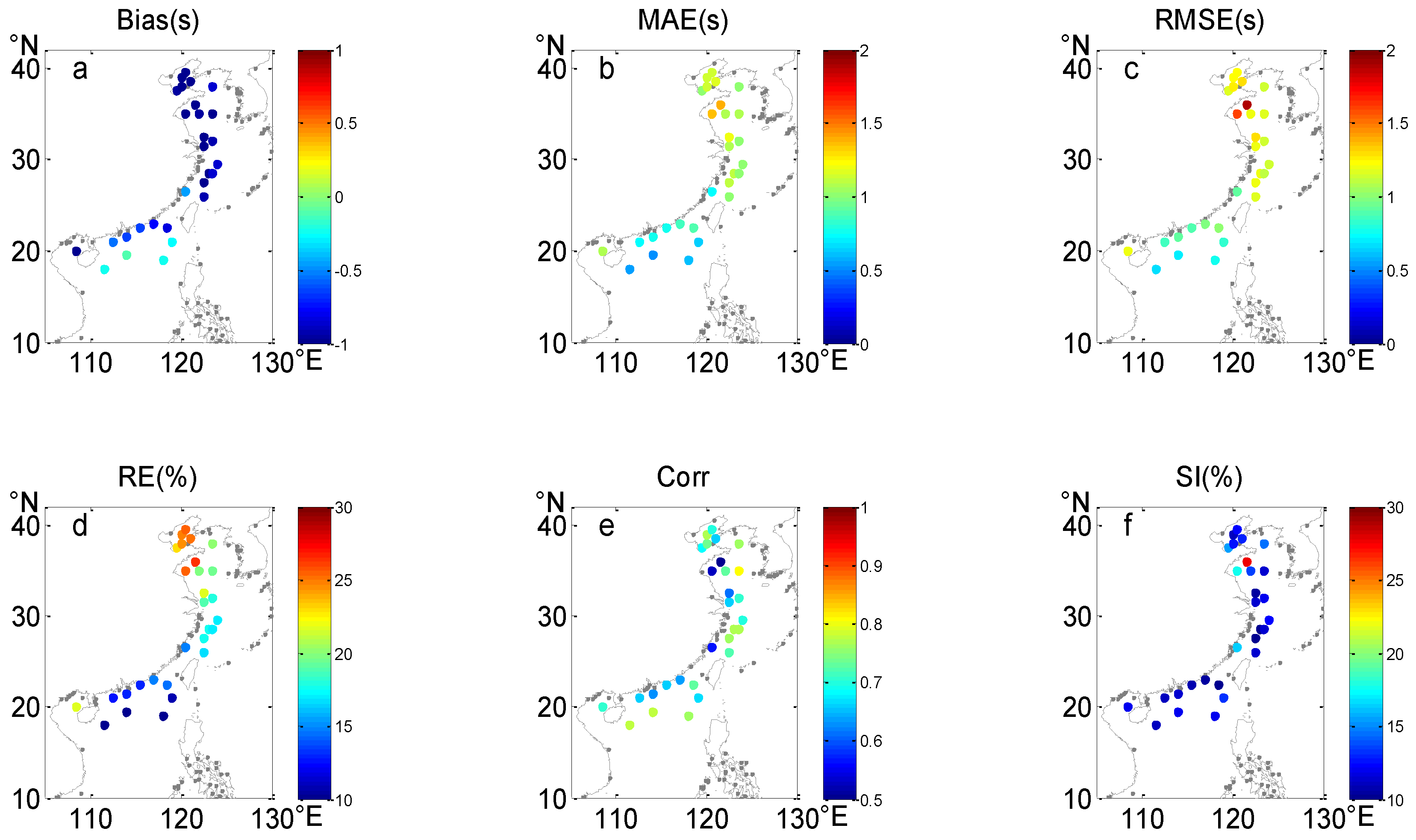
Figure 9 and Figure 10, respectively, show the error distribution of the Hs and Tm 0–24 h forecasts at each buoy position in the offshore waters of China, while Table 3 and Table 4, respectively, summarize the error parameters of forecasting for different sea areas to explore the spatial distribution characteristics of the model’s forecasting accuracy. In semi-enclosed sea areas such as the Bohai Sea, Yellow Sea, and Beibu Gulf, the average Hs values observed by buoys in 2022 were all slight waves below 1 m. The model showed a certain negative Bias for Hs forecasting, with the largest negative Bias near Liaodong Bay of the Bohai Sea (−0.18 m). The reason for the Hs underestimation of the model in these sea areas may lie in the shallow water depths, while the influence of nonlinear interactions on wind wave growth was more pronounced than in other sea areas. In areas with shallow water depths, the terrain had a significant impact, but the terrain data used in the model were not accurate enough for these semi-enclosed waters. In addition, when affected by cold air in winter, a significant air–sea temperature difference in the northern sea areas was observed, and the atmospheric stratification was unstable. Due to the failure to reflect the influence of the atmospheric stratification stability on the growth rate of wind waves, the Hs forecasts in the northern sea areas were often underestimated, which constituted another key reason. The RMSE values of the Hs forecasts in the Bohai Sea, Yellow Sea, and Beibu Gulf were within 0.3 m, and the RE values were less than 20%. However, the SI values of the Hs forecasts were relatively high, reaching 37% in the Bohai Sea, and nearly 30% in the Yellow Sea and Beibu Gulf. This was consistent with the performance of the driving wind field, which also exhibited significant SI values in the Bohai Sea, Yellow Sea, and Beibu Gulf. In isolated basins and coastal areas, the complex terrain also led to a decrease in the wave models’ performance. The average Hs values observed by buoys in the East and South China Seas in 2022 were moderate waves of 1.5–2 m. The forecasting of the Hs in the East China Sea by the model showed a slight positive Bias (0.01 m), RMSE within 0.3 m, relatively low RE (approximately 14%), and SI within 20%. The forecasting of the Hs in the South China Sea by the model showed a significant positive Bias (0.17 m), RMSE of 0.38 m, RE of 16%, and SI of less than 20%.
For the Tm forecasting, semi-enclosed sea areas such as the Bohai Sea, Yellow Sea, and Beibu Gulf had the characteristics of less swell propagation, short fetch length, and insufficient wave development compared to open sea areas. Influenced by continental weather processes, wind waves in such areas were featured by fast growth and dissipation, and most were short-period wind waves, with wave periods generally smaller than those in open sea areas. The average Tm values observed by buoys in 2022 were around 5 s, and the Tm forecasts by the ocean wave model showed more obvious underestimation and greater forecasting errors than those in the East and South China Seas. In consideration of a wide continental shelf and shadowing effect of peripheral island chains, the proportion of short-period wind waves in the East China Sea was higher than the oceans. The South China Sea had a greater depth and more swells. Viewed from various statistical items, the model performed best in forecasting the Tm in the South China Sea, with a Bias of −047 s, RMSE of less than 1 s, RE of 12%, and SI of 11.2%, followed by the forecasting performance of the model in the East China Sea.

3.2. Evaluation of Forecasting Performance in Global Ocean Waters

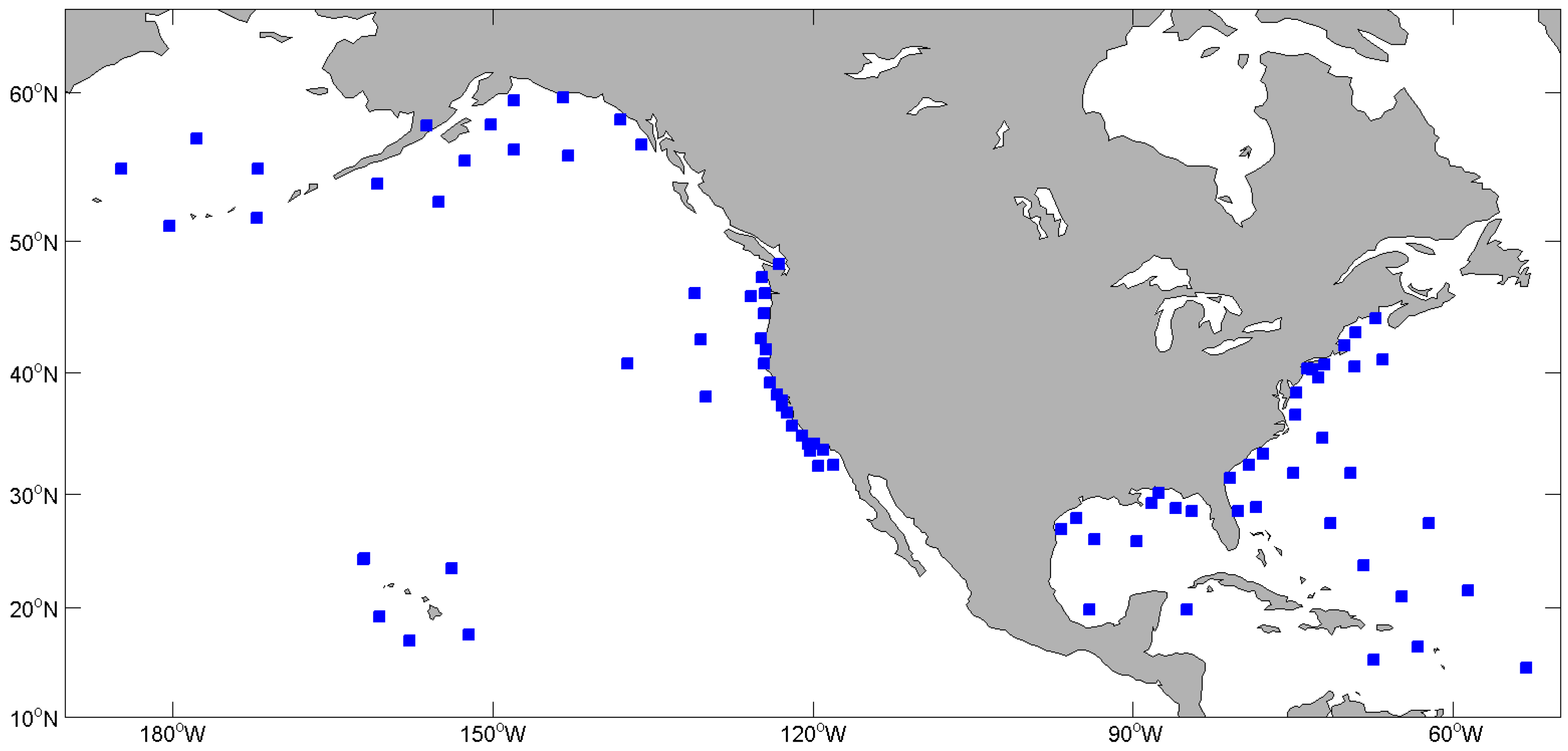
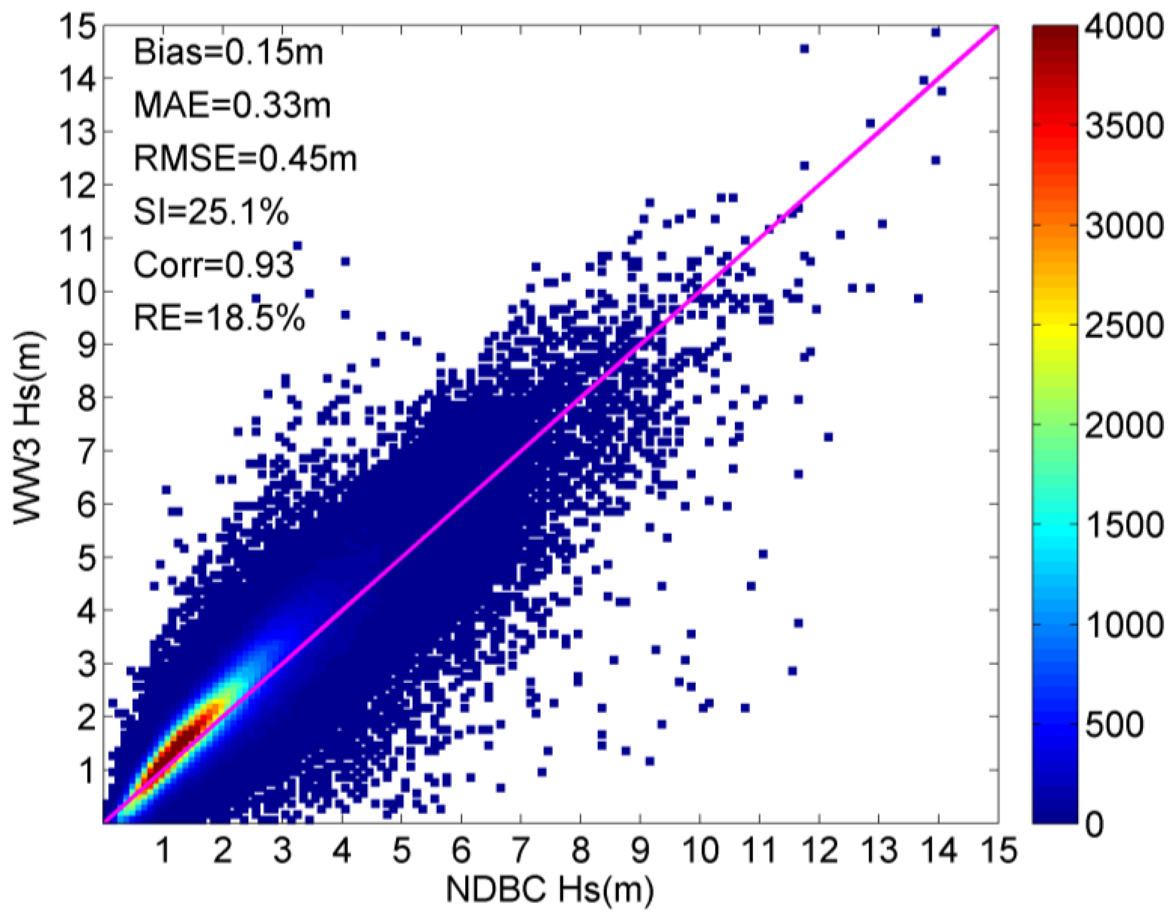
We collected data from nearly 100 NDBC buoys to validate the forecasting performance of the global ocean. Most of the buoys were located in the Pacific and Atlantic Oceans; their positions are shown in Figure 11, and the test results in Figure 12. The model had a strong forecasting effect in the global ocean, with an Hs prediction Bias of 0.15 m, RMSE of 0.45 m, RE of 18.5%, and Corr of 0.93. Further analyses were conducted on the statistical results of different sea areas (Table 5); the model showed negative Bias values in the Gulf of Mexico and the East Coast, a slight positive Bias (0.1 m) in the western Atlantic Ocean, and significant positive Bias values (0.28 and 0.29 m) in the tests by using Pacific buoys located on the West Coast and Hawaii. The SI values were larger in the Gulf of Mexico and nearshore areas, and smaller in the offshore waters.
The spatial validation of the model’s forecasting performance in global ocean waters was conducted using the along-track Hs data of the Jason-3 satellite altimeter. The distributions of the Bias, RMSE, and RE are shown in Figure 13. According to the analysis results, significant positive Bias values were observed in most of the global waters, especially in the Southern Ocean (also with maximum RMSE), which were related to the swell events generated by storms there. In the East Pacific Ocean and East Indian Ocean dominated by swells, significant positive Bias values associated with excessive swell propagation from the Southern Ocean were also observed. The RE values presented by the forecasts in these regions were also relatively high. The reason for the overestimation of the wave model may lie in the dissipation source function term, wind forcing, and unrecognizable terrain such as islands and atolls [7,35]. The negative Bias values of the model mainly occurred on the east coast and in relatively isolated basins, such as the Sea of Japan and Gulf of Mexico. Compared to the west coast, these areas were less susceptible to the swell propagation errors of the Southern Ocean, but more susceptible to strong fast weather processes such as cold air outbreaks, cyclone disturbances, and frontal systems.
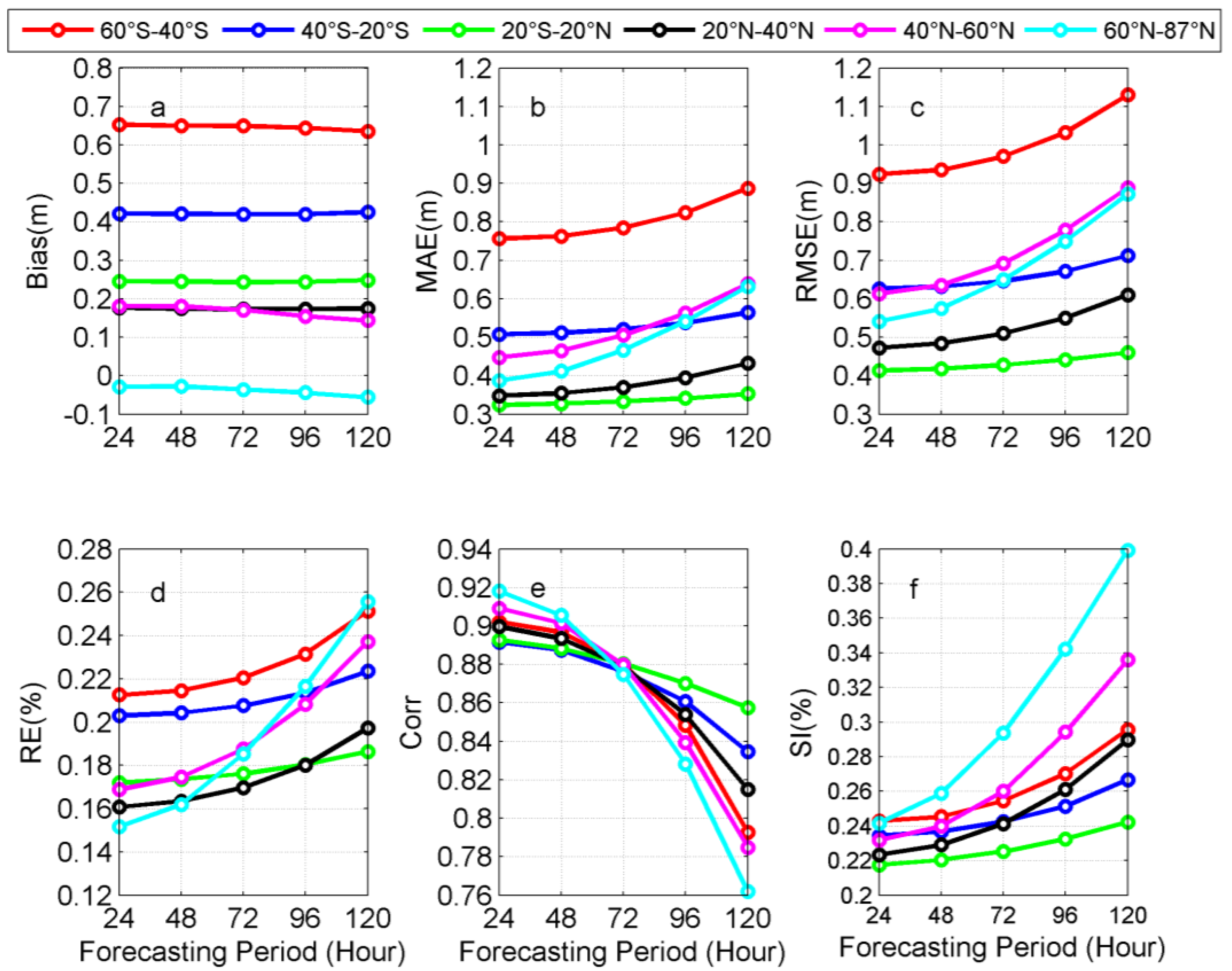
The RMSE distribution of the Hs forecasts showed that the model’s performance varied in different latitude zones. Figure 14 further quantitatively analyzes the error distributions of the model in Hs forecasting at different latitudes during the 5-day forecast period. For high-latitude Arctic waters, due to the limited amount of data from a single satellite, the forecasting performance in the Arctic waters was evaluated using the fusion satellite Hs data from the CMEMS. The forecasting Bias values changed little with the growth of the forecast period yet exhibited significant latitude differences. The Southern Ocean (60°S–40°S, red line) showed a significant positive Bias of about 0.6 m, and the highest RMSE of the Hs forecasts. The positive Bias values decreased toward the north, and the Arctic waters (60°N–87°N, cyan line) showed a slight negative Bias. The RMSE of the Hs forecasts was the smallest in tropical waters (20°S–20°N, green line). The high-latitude waters north of 40°N (magenta and cyan lines) showed high SI values for the forecasts after 72 h. Regardless of the statistical items, the accuracy of the Hs forecasting in the Arctic waters decreased fastest with the increase in the validity period, especially after 72 h. On the contrary, the forecasting accuracy of the model for tropical waters changed slowest during the forecast period.

4. Discussion

In this paper, in situ buoy observations and remote sensing data were used to perform a detailed evaluation of the NMEFC’s operational global ocean wave forecasting results for 2022, to help comprehensively understand the forecasting model’s error characteristics and provide important feedback on the forecasting quality for model researchers, users, and operational forecasters.
According to the research findings, the forecasting results of the model showed a certain degree of positive Bias in most global sea areas. Wu [36] found that the addition of satellite data assimilation significantly improved the forecasting system Bias, especially in areas dominated by swells. In the next phase of work, it is advisable to consider adding a data assimilation system, and to replace the wind forcing field with a more accurate one. In the offshore areas of China, such as the Bohai and Yellow Seas, the Hs had always been underestimated. When affected by cold air in winter, a significant air–sea temperature difference in the northern sea area was observed, and the atmospheric stratification was unstable. Due to the failure to reflect the impact of the atmospheric stratification stability on the growth rate of wind waves, the ocean wave model may underestimate the Hs. In an alternate version of the wave forecasting system, by studying the impact of atmospheric stratification stability changes caused by air–sea temperature differences on the growth rate of wind waves, corrections were made in the model’s wind energy input term, to help solve the problem of wave height underestimations in the northern sea areas during winter. In isolated basins and complex waters adjacent to the shore, complex terrain may also lead to a decrease in the performance of the wave model (high SI); thus, higher resolution calculations are needed for these areas. In another version of the system, SMC [37,38,39,40] multi-grids were applied to reduce the impact of complex terrain, so that multi-layer resolution refinement could help to analyze small islands and fine coastline [23,41], thereby further improving the forecasting level of nearshore sea waves. More consideration will be given to the study of ice–wave interactions for a further improvement in the forecasting performance in Arctic waters.

5. Conclusions

China’s NMEFC has developed a global ocean wave numerical forecasting system based on the WAVEWATCH III 6.07 wave model. In this paper, a detailed evaluation of the operational forecasting results for 2022 was conducted using China’s offshore buoy observations and satellite remote sensing data to ensure the model’s reliability. The evaluation of the forecasting performance in China’s offshore waters included two wave parameters—Hs and Tm—and that in global ocean and Arctic waters focused on the Hs.
Overall, the Hs was accurately simulated by the model. The 0–24 h Hs forecasts through China’s offshore buoy inspects showed a Bias of 0.02 m, RMSE of 0.3 m, RE of 16%, and Corr reaching 0.95. As the forecast period increased, the accuracy of the Hs forecasting decreased. The model tended to underestimate the Hs values in autumn and winter and overestimate them in spring and summer. The Corr, RE, and SI of the Hs forecasts in autumn and winter were superior to those in spring and summer. The forecasting Bias values of the model were positive for most of the Hs ranges, and the model only slightly underestimated the Hs below 1 m. Within the Hs range of 1–7 m, as the Hs values increased, the model’s overestimation of them became increasingly severe. For high Hs values, the SI forecast by the model tended to be lower. In terms of spatial distribution, negative Bias values were observed in the Hs forecasts for semi-enclosed sea areas such as the Bohai Sea, Yellow Sea, and Beibu Gulf, and high SI values were also observed, with the largest negative Bias near the Liaodong Bay of the Bohai Sea (−0.18 m), a slight positive Bias in the East China Sea (0.01 m), and a significant positive Bias in the South China Sea (0.17 m).
For the Tm forecasting in China’s offshore areas, the model had a negative Bias of −0.79 s, tending to underestimate the Tm. Compared with the Hs, the Tm forecasting accuracy during the 5-day forecast period showed a smaller decrease over time. The model also exhibited obvious seasonal characteristics in the Tm forecasting error. The underestimations of the Tm by the model in autumn and winter were more pronounced than in spring and summer, and the Corr and SI of the Tm forecasts in autumn and winter were also better overall. As the Tm value increased, the negative Bias increased, and the wave model tended to underestimate the big wave period even more. In terms of regional distribution, the Tm values in semi-enclosed sea areas such as the Bohai Sea, Yellow Sea, and Beibu Gulf were more significantly underestimated than in the East and South China Seas, also with greater forecasting errors. The model performed best in Tm forecasting for the South China Sea, followed by the East China Sea.
According to the evaluation results, significant positive Bias values were observed in most of the global waters, especially in the Southern Ocean, East Pacific Ocean, and East Indian Ocean. The negative Bias values mainly occurred on the east coast and in relatively isolated basins, such as the Sea of Japan and Gulf of Mexico, and the SI values were larger in the isolated basins and nearshore areas, whereas they were smaller in the offshore waters. The forecasting Bias values showed significant latitude differences. The Southern Ocean showed a significant positive Bias of about 0.6 m, and the largest RMSE for the Hs forecasts. The positive Bias values decreased toward the north, and the Arctic waters showed a slight negative Bias. The RMSE of the Hs forecasts was the smallest in tropical waters. The high-latitude waters north of 40°N showed high SI values for forecasts after 72 h. The accuracy of the Hs forecasting in the Arctic waters decreased fastest with the increase in the prediction period, especially after 72 h. On the contrary, the forecasting accuracy of the model for tropical waters changed slowest during the forecast period.
In summary, the global wave model has high reliability and can meet the current operational forecasting needs. The error distribution characteristics of the model found in the evaluation will provide a reference basis for model research and improvement in the future. The accuracy and performance of ocean wave forecasting can be further improved through methods such as parameterization scheme adjustment and data assimilation.

Author Contributions

Conceptualization, H.W. and J.W. (Jiuke Wang); data curation, J.W. (Juanjuan Wang); formal analysis, M.W.; investigation, Y.W.; methodology, M.W.; resources, M.W.; software, Q.C.; supervision, H.W.; validation, M.W. and J.W. (Juanjuan Wang); visualization, M.W.; writing—original draft, M.W.; writing—review and editing, H.W. All authors have read and agreed to the published version of the manuscript.

Funding

This research was funded by the National Key Research and Development Program of China, Grant No. 2022YFC2806603 and No. 2021YFC3101605.

Data Availability Statement

The Jason-3 altimeter data can be downloaded from https://aviso.altimetry.fr/en/data/data-access/ftp.html (accessed on 6 September 2024). The integrated satellite data can be obtained from https://data.marine.copernicus.eu/product/WAVE_GLO_PHY_SWH_L3_NRT_014_001/services (accessed on 6 September 2024). The NDBC buoys data can be obtained from https://www.ndbc.noaa.gov/ (accessed on 20 June 2024). As for the model data used in this paper, which require a large storage facility, these are available upon request to the corresponding author.

Acknowledgments

The authors would like to thank NOAA/NCEP for providing the WAVEWATCH III source code and wind data. The authors would also like to acknowledge the data support from GEBCO, AVISO, CMEMS, and NDBC.

Conflicts of Interest

The authors declare no conflicts of interest.

References

  1. WAMDI Group. The WAM Model—A Third Generation Ocean Wave Prediction Model. J. Phys. Oceanogr. 1988, 18, 1775–1810. [Google Scholar] [CrossRef]
  2. Komen, G.J.; Cavaleri, L.; Donelan, M.; Hasselmann, K.; Hasselmann, S.; Janssen, P.A.E.M. Dynamics and Modelling of Ocean Waves; Cambridge University Press: Cambridge, UK, 1994; ISBN 0-521-47047-1. [Google Scholar]
  3. Tolman, H.L. A Third-Generation Model for Wind Waves on Slowly Varying, Unsteady and Inhomogeneous Depth and Currents. J. Phys. Oceanogr. 1991, 21, 782–797. [Google Scholar] [CrossRef]
  4. Tolman, H.L. User Manual and System Documentation of WAVEWATCH IIITM version 3.14. Tech. Note MMAB Contrib. 2009, 276, 194. [Google Scholar]
  5. Booij, N.; Ris, R.C.; Holthuijsen, L.H. A Third-Generation Wave Model for Coastal Regions: 1. Model Description and Validation. J. Geophys. Res. Ocean. 1999, 104, 7649–7666. [Google Scholar] [CrossRef]
  6. Bidlot, J.R. Present Status of Wave Forecasting at ECMWF. In Workshop on Ocean Waves; ECMWF: Reading, UK, 2012. [Google Scholar]
  7. Janssen, P.A.E.M.; Bidlot, J.R. Progress in Operational Wave Forecasting. Procedia IUTAM 2018, 26, 14–29. [Google Scholar] [CrossRef]
  8. ECMWF. IFS Documentation CY45R1—Part VII: ECMWF Wave Model; ECMWF: Reading, UK, 2018. [Google Scholar] [CrossRef]
  9. Campos, R.M.; Alves, J.H.G.M.; Penny, S.G.; Krasnopolsky, V. Assessments of Surface Winds and Waves from the NCEP Ensemble Forecast System. Weather Forecast. 2018, 33, 1533–1546. [Google Scholar] [CrossRef]
  10. Chen, H.S. Ensemble Prediction of Ocean Waves at NCEP. In Proceedings of the 28th Ocean Engineering Conference, Taipei, Taiwan, China, 30 November–2 December 2006; pp. 25–37. [Google Scholar]
  11. Cao, D.; Chen, H.S.; Tolman, H. Verification of Ocean Wave Ensemble Forecasts at NCEP. In Proceedings of the 10th International Workshop on Wave Hindcasting and Forecasting and Coastal Hazard Symposium, Oahu, HI, USA, 11–16 November 2007; Available online: http://www.waveworkshop.org/10thWaves/ProgramFrameset.htm (accessed on 18 July 2023).
  12. Alves, J.H.G.M.; Chawla, A.; Tolman, H.L.; Schwab, D.; Lang, G.; Mann, G. The Operational Implementation of a Great Lakes Wave Forecasting System at NOAA/NCEP. Weather Forecast. 2014, 29, 1473–1497. [Google Scholar] [CrossRef]
  13. Aouf, L.; Lefèvre, J.M. On the Impact of the Assimilation of SARAL/AltiKa Wave Data in the Operational Wave Model MFWAM. Mar. Geod. 2015, 38, 381–395. [Google Scholar] [CrossRef]
  14. Li, J.G.; Saulter, A. Unified Global and Regional Wave Model on a Multi-Resolution Grid. Ocean Dyn. 2014, 64, 1657–1670. [Google Scholar] [CrossRef]
  15. Seemanth, M.; Remya, P.G.; Bhowmick, S.A.; Sharma, R.; Balakrishnan Nair, T.M.; Kumar, R.; Chakraborty, A. Implementation of Altimeter Data Assimilation on a Regional Wave Forecasting System and Its Impact on Wave and Swell Surge Forecast in the Indian Ocean. Ocean Eng. 2021, 237, 109585. [Google Scholar] [CrossRef]
  16. Wan, L.; Liu, Y.; Ling, T. Development of a Global High-Resolution Marine Dynamic Environmental Forecasting System. Atmos. Ocean. Sci. Lett. 2018, 11, 379–387. [Google Scholar] [CrossRef]
  17. Wang, H.; Wan, L.; Qin, Y.; Wang, Y.; Yang, X.; Liu, Y.; Xing, J.; Chen, L.; Wang, Z.; Zhang, T.; et al. Development and Application of the Chinese Global Operational Oceanography Forecasting System. Adv. Earth Sci. 2016, 31, 1090–1104. [Google Scholar]
  18. Wang, Y.; Yu, Z. Validation of Impact of Assimilation of Altimeter Satellite Significant Wave Height on Wave Forecast in the Northwest Pacific. Acta Oceanol. Sin. 2009, 31, 1–8. [Google Scholar] [CrossRef]
  19. Bidlot, J.R.; Holmes, D.J.; Wittmann, P.A.; Lalbeharry, R.; Chen, H.S. Inter-comparison of the Performance of Operational Ocean Wave Forecasting Systems with Buoy Data. Weather Forecast. 2002, 17, 287–310. [Google Scholar] [CrossRef]
  20. Bidlot, J.R.; Holt, M. Verification of Operational Global and Regional Wave Forecasts Systems against Measurements from Moored Buoys; JCOMM Tech. Rep. 2006, 30, WMO-TD-1333; WMO: Geneva, Switzerland; IOC: Geneva, Switzerland, 2006; 11p.
  21. Bidlot, J.R.; Li, J.G.; Wittmann, P.; Fauchon, M.; Chen, H.; Lefevre, J.M.; Bruns, T.; Greenslade, D.; Ardhuin, F.; Kohno, N.; et al. Inter-Comparison of Operational Wave Forecasting Systems. In Proceedings of the 10th International Workshop on Wave Hindcasting and Forecasting and Coastal Hazard Symposium, Oahu, HI, USA, 11–16 November 2007. Available online: http://www.waveworkshop.org/10thWaves/ProgramFrameset.htm (accessed on 19 July 2023).
  22. WMO Lead Centre for Wave Forecast Verification. Intercomparison of Operational Wave Forecasting Systems Against In-Situ Observations for JJA 2023—00 and 12UTC Runs, Part I: Significant Wave Height; ECMWF: Reading, UK, 2023; 61p, Available online: https://confluence.ecmwf.int/display/WLW/Significant+wave+height?prview=/116958920/348807936/LCWFV_swh_report_12_JJA2023.pdf (accessed on 19 December 2023).
  23. Valiente, N.G.; Saulter, A.; Gomez, B.; Bunney, C.; Li, J.G.; Palmer, T.; Pequignet, C. The Met Office Operational Wave Forecasting System: The Evolution of the Regional and Global Models. Geosci. Model Dev. 2023, 16, 2515–2538. [Google Scholar] [CrossRef]
  24. Bernier, N.B.; Alves, J.H.; Tolman, H.; Chawla, A.; Peel, S.; Pouliot, B.; Bélanger, J.M.; Pellerin, P.; Lépine, M.; Roch, M. Operational Wave Prediction System at Environment Canada: Going Global to Improve Regional Forecast Skill. Weather Forecast. 2016, 31, 353–370. [Google Scholar] [CrossRef]
  25. Michalis, R.; Anna, Z.; Gerasimos, K. Implementation and Validation of a New Operational Wave Forecasting System of the Mediterranean Monitoring and Forecasting Centre in the framework of the Copernicus Marine Environment Monitoring Service. Nat. Hazards Earth Syst. Sci. 2018, 18, 2675–2695. [Google Scholar] [CrossRef]
  26. Remya, P.G.; Rabi Ranjan, T.; Sirisha, P.; Harikumar, R.; Balakrishnan Nair, T.M. Indian Ocean Wave Forecasting System for Wind Waves: Development and Its Validation. J. Oper. Oceanogr. 2020, 14, 1–16. [Google Scholar] [CrossRef]
  27. The WAVEWATCH III Development Group (WW3DG). User Manual and System Documentation of WAVEWATCH III Version 6.07; Tech. Note 333; NOAA/NWS/NCEP/MMAB: College Park, MD, USA, 2019; Appendices, 465p. [Google Scholar]
  28. Yang, J.; Zhang, J.; Jia, Y.; Fan, C.; Cui, W. Validation of Sentinel-3A/3B and Jason-3 Altimeter Wind Speeds and Significant Wave Heights Using Buoy and ASCAT Data. Remote Sens. 2020, 12, 2079. [Google Scholar] [CrossRef]
  29. Li, X.; Xu, Y.; Liu, B.; Lin, W.; He, Y.; Liu, J. Validation and Calibration of Nadir SWH Products from CFOSAT and HY-2B with Satellites and In Situ Observations. J. Geophys. Res. Ocean. 2021, 126, e2020JC016689. [Google Scholar] [CrossRef]
  30. Sepulveda, H.H.; Queffeulou, P.; Ardhuin, F. Assessment of SARAL/AltiKa Wave Height Measurements Relative to Buoy, Jason-2, and Cryosat-2 Data. Mar. Geod. 2015, 38, 449–465. [Google Scholar] [CrossRef]
  31. Young, I.R.; Zieger, S.; Babanin, A.V. Global Trends in Wind Speed and Wave Height. Science 2011, 332, 451–455. [Google Scholar] [CrossRef]
  32. WMO Lead Centre for Wave Forecast Verification. Intercomparison of Operational Wave Forecasting Systems Against In-Situ Observations for JJA 2023—00 and 12UTC Runs, Part III: 10 Meter Wind Speed; ECMWF: Reading, UK, 2023; 61p, Available online: https://confluence.ecmwf.int/display/WLW/Wind+speed?preview=/116958928/373758446/LCWFV_10ff_report_12_SON2023.pdf (accessed on 20 December 2023).
  33. Wang, J.; Li, B.; Gao, Z.; Wang, J. Comparison of ECMWF Significant Wave Height Forecasts in the China Sea with Buoy Data. Weather Forecast. 2019, 34, 1693–1704. [Google Scholar] [CrossRef]
  34. Ardhuin, F.; Orfila, A. Wind waves. In New Frontiers in Operational Oceanography; Chassignet, E.P., Pascual, A., Tintoré, J., Verron, J., Eds.; GODAE: Mallorca, Spain, 2018; pp. 393–422. [Google Scholar]
  35. Tolman, H.L. Treatment of Unresolved Islands and Ice in Wind Wave Models. Ocean Model. 2003, 5, 219–231. [Google Scholar] [CrossRef]
  36. Wu, M.; Wang, H.; Wan, L.; Wang, J.; Wang, Y.; Wang, J. The Impacts of the Application of the Ensemble Optimal Interpolation Method in Global Ocean Wave Data Assimilation. Atmosphere 2023, 14, 818. [Google Scholar] [CrossRef]
  37. Li, J.G. Global Transport on a Spherical Multiple-Cell Grid. Mon. Weather Rev. 2011, 139, 1536–1555. [Google Scholar] [CrossRef]
  38. Li, J.G. Propagation of Ocean Surface Waves on a Spherical Multiple-Cell Grid. J. Comput. Phys. 2012, 231, 8262–8277. [Google Scholar] [CrossRef]
  39. Li, J.G. Hybrid Multi-Grid Parallelisation of WAVEWATCH III Model on Spherical Multiple-Cell Grids. J. Parallel Distr. Com. 2022, 167, 187–198. [Google Scholar] [CrossRef]
  40. Hou, F.; Gao, Z.; Li, J.; Yu, F. An Efficient Algorithm for Generating a Spherical Multiple-Cell Grid. Acta Oceanol. Sin. 2022, 41, 41–50. [Google Scholar] [CrossRef]
  41. Saulter, A.; Bunney, C.; Li, J.G.; Palmer, T. Process and Resolution Impacts on UK Coastal Wave Predictions from Operational Global-Regional Wave Models. In Proceedings of the 1st International Workshop on Waves, Storm Surges and Coastal Hazards Incorporating the 15th International Waves Workshop, Liverpool, UK, 10–15 September 2017. Available online: http://www.waveworkshop.org/15thWaves/index.htm (accessed on 19 July 2023).
Figure 1. The flowchart of the global ocean wave forecasting system.
Remotesensing 16 03535 g001
Figure 2. Comparisons of China’s offshore buoy observations and 0–24 h model’s forecasting results. (a) Significant wave height (Hs) inspection; (b) mean wave period (Tm) inspection; (c) 10 m wind speed inspection. The magenta lines are diagonal lines, and the color codes represent the amounts of data.
Remotesensing 16 03535 g002
Figure 3. Hs inspections for different prediction periods. (a) Deviation (Bias); (b) mean absolute error (MAE); (c) root mean square error (RMSE); (d) relative error (RE); (e) correlation coefficient (Corr); (f) scatter index (SI).
Remotesensing 16 03535 g003
Figure 4. Tm inspections for different prediction periods. (a) Bias; (b) MAE; (c) RMSE; (d) RE; (e) Corr; (f) SI.
Remotesensing 16 03535 g004
Figure 5. Distributions of monthly Hs forecasting errors. (a) Bias; (b) MAE; (c) RMSE; (d) RE; (e) Corr; (f) SI.
Remotesensing 16 03535 g005
Figure 6. Distributions of monthly Tm forecasting errors. (a) Bias; (b) MAE; (c) RMSE; (d) RE; (e) Corr; (f) SI.
Remotesensing 16 03535 g006
Figure 7. Distributions of Hs forecasting errors in different Hs ranges. (a) Bias; (b) RMSE; (c) RE; (d) SI.
Remotesensing 16 03535 g007
Figure 8. Distributions of Tm forecasting errors in different Tm ranges. (a) Bias; (b) RMSE; (c) RE; (d) SI.
Remotesensing 16 03535 g008
Figure 9. Distributions of Hs forecasting errors at different buoy positions. (a) Bias; (b) MAE; (c) RMSE; (d) RE; (e) Corr; (f) SI.
Remotesensing 16 03535 g009
Figure 10. Distributions of Tm forecasting errors at different buoy positions. (a) Bias; (b) MAE; (c) RMSE; (d) RE; (e) Corr; (f) SI.
Remotesensing 16 03535 g010
Figure 11. Locations of buoys from National Data Buoy Center (NDBC).
Remotesensing 16 03535 g011
Figure 12. Comparisons of NDBC buoy observations and 0–24 h model’s forecasting results. The magenta line is a diagonal line, and the color code represents the amounts of data.
Remotesensing 16 03535 g012
Figure 13. Global error distributions of Hs forecasting. (a) Bias distribution; (b) RMSE distribution; (c) RE distribution.
Remotesensing 16 03535 g013
Figure 14. Distributions of Hs forecasting errors in different latitude ranges. (a) Bias; (b) MAE; (c) RMSE; (d) RE; (e) Corr; (f) SI.
Remotesensing 16 03535 g014
Table 1. Statistics of Hs forecasting errors in different seasons.
EntriesBuoy Hs (m)WW3 Hs (m)Bias (m)MAE (m)RMSE (m)RE (%)CorrSI (%)
Entire year187,0521.321.340.020.250.3316.280.9525.41
Spring47,0921.121.190.070.230.3116.490.9426.53
Summer47,6930.961.030.070.230.3119.370.9131.52
Autumn48,3031.561.53−0.030.250.3414.440.9622.14
Winter43,9641.641.59−0.050.270.3714.950.9521.75
Table 2. Statistics of Tm forecasting errors in different seasons.
EntriesBuoy Tm (s)WW3 Tm (s)Bias (s)MAE (s)RMSE (s)RE (%)CorrSI (%)
Entire year125,3615.524.73−0.790.941.1217.380.7613.93
Spring29,5205.444.71−0.730.891.0916.650.7514.50
Summer30,6505.254.65−0.600.861.0316.650.6915.64
Autumn34,2035.784.88−0.901.001.2117.650.7513.80
Winter30,9885.594.67−0.921.001.1418.570.8311.75
Table 3. Statistics of Hs forecasting errors in different sea areas.
EntriesBuoy Hs (m)WW3 Hs (m)Bias (m)MAE (m)RMSE (m)RE (%)CorrSI (%)
Bohai Sea27,1500.710.62−0.090.210.2819.100.8837.57
Yellow Sea50,6680.950.87−0.080.210.2717.220.9128.02
East China Sea41,5791.541.550.010.220.2914.070.9319.45
South China Sea60,2951.791.960.170.290.3816.050.9618.33
Beibu Gulf77720.920.87−0.050.20.2818.220.9229.74
Table 4. Statistics of Tm forecasting errors in different sea areas.
EntriesBuoy Tm (s)WW3 Tm (s)Bias (s)MAE (s)RMSE (s)RE (%)CorrSI (%)
Bohai Sea13,0864.433.38−1.051.081.2123.200.7613.32
Yellow Sea29,2305.184.09−1.091.181.3921.800.6816.30
East China Sea30,8215.834.90−0.931.031.1516.680.7411.23
South China Sea47,8675.95.43−0.470.700.8412.000.7411.21
Beibu Gulf43264.83.76−1.041.071.1921.810.7212.02
Table 5. Statistics of Hs forecasting errors in different sea areas using NDBC buoys.
Bias (m)MAE (m)RMSE (m)RE (%)CorrSI (%)
Gulf of Mexico−0.080.220.3116.880.9128.98
East Coast−0.050.240.3516.380.9125.55
Atlantic Ocean0.100.220.3112.040.9217.25
West Coast0.280.430.5621.150.9126.04
Hawaii0.290.330.4215.910.9219.75
Disclaimer/Publisher’s Note: The statements, opinions and data contained in all publications are solely those of the individual author(s) and contributor(s) and not of MDPI and/or the editor(s). MDPI and/or the editor(s) disclaim responsibility for any injury to people or property resulting from any ideas, methods, instructions or products referred to in the content.