Article

A Novel Framework for Spatiotemporal Susceptibility Prediction of Rainfall-Induced Landslides: A Case Study in Western Pennsylvania

1
Department of Civil and Environmental Engineering, The Pennsylvania State University, University Park, PA 16802, USA
2
Department of Civil Engineering, The City College of New York, New York, NY 10031, USA
3
Department of Civil and Environmental Engineering, The University of Utah, Salt Lake City, UT 84112, USA
*
Author to whom correspondence should be addressed.
Remote Sens. 2024, 16(18), 3526; https://doi.org/10.3390/rs16183526
Submission received: 11 July 2024 / Revised: 9 September 2024 / Accepted: 14 September 2024 / Published: 23 September 2024

Abstract

:
Landslide susceptibility measures the probability of landslides occurring under certain geo-environmental conditions and is essential in landslide hazard assessment. Landslide susceptibility mapping (LSM) using data-driven methods applies statistical models and geospatial data to show the relative propensity of slope failure in a given area. However, due to the rarity of multi-temporal landslide inventory, conventional data-driven LSMs are primarily generated by spatial causative factors, while the temporal factors remain limited. In this study, a spatiotemporal LSM is carried out using machine learning (ML) techniques to assess rainfall-induced landslide susceptibility. To achieve this, two landslide inventories are collected for southwestern Pennsylvania: a spatial inventory and a multi-temporal inventory, with 4543 and 223 historical landslide samples, respectively. The spatial inventory lacks the information to describe landslide temporal distribution; there are insufficient samples in the temporal inventory to represent landslide spatial distribution. A novel paradigm of data augmentation through non-landslide sampling based on domain knowledge is applied to leverage both spatial and temporal information for ML modeling. The results show that the spatiotemporal ML model using the proposed data augmentation predicts well rainfall-induced landslides in space and time across the study area, with a value of 0.86 of the area under the receiver operating characteristic curve (AUC), which makes it an effective tool in rainfall-induced landslide hazard mitigation and forecasting.

1. Introduction

Among various natural hazards, landslides are among the most destructive geologic hazards that can destroy utilities, structures, and transportation routes, and cause travel delays and other adverse effects. Landslides are expected to occur more frequently in the future with increased urbanization, deforestation, and precipitation intensity due to global climate change. For landslide-prone areas, the importance of landslide susceptibility mapping (LSM) lies in its ability to provide a scientific basis for landslide risk assessment and management. The methods of LSM can be broadly categorized into three types: knowledge-guided methods, physics-based methods, and data-driven methods [1,2,3,4,5]. These methodologies, as well as comparisons of them, have been widely studied [6,7,8,9,10,11,12]. Typically, large-scale LSM involves large amounts of data due to complex variables, making data-driven methods more suitable for the tasks associated with regional LSM compared to other physical methods [13,14].
In recent years, the big data era has brought enormous benefits to society and different sectors. Machine learning (ML) techniques, as flourishing data-driven methods, have been applied to LSM. Reichenbach et al. [15] reviewed published works on various aspects of LSM with ML techniques; they summarized the recent practices and strengths in LSM and recommended that dynamic climate-related variables should be included. Huang et al. [16] reviewed the applications of support vector machine (SVM) in LSM. By comparing SVM with other models commonly used in LSM, they suggested that ample data should be included in the database for training satisfactory models, and comprehensive landslide causative factors should be involved in the analysis. Merghadi et al. [17] summarized the popular ML techniques available for LSM and highlighted the advantages and disadvantages of each model through a case study in Algeria. Moziihrii et al. [18] conducted a comprehensive literature survey and showed the current trend of LSM using ML techniques. Their survey reveals that as more landslide data becomes available, the number of studies focusing on ML-based LSM increases. In addition, while conventional ML methods can achieve acceptable prediction results, newly explored ML technologies are also being considered to generate more reliable LSMs in recent years.
Previous studies indicate that ML-based methods are effective for assessing complex relationships between landslide occurrence and causative factors. Nevertheless, conventional LSMs are static, only focusing on the relationships between landslide occurrences and spatial environments. Unlike static spatial models, temporal assessments capture trends, patterns, and variations of landslide susceptibility. In recent years, researchers have tried to combine the landslide-triggering rainfall thresholds with LSM to provide temporal predictions of landslides. For example, Rosi et al. [19] determined a national intensity-duration (ID) rainfall threshold and several local rainfall thresholds for Slovenia. The model performance indicates that all thresholds have an excellent capability to avoid false alarms. Peruccacci et al. [20] defined empirical rainfall duration (ED) thresholds for different environmental subdivisions of Italy. Huang et al. [21] combined the landslide spatial probability using ML models with the temporal probability obtained from rainfall thresholds to assess landslide risk in Xunwu County, China. However, rainfall thresholds for landslides are highly site-specific as they are mainly influenced by local topography and soil conditions. Since rainfall thresholds vary regionally, they are unsuitable for large-scale landslide susceptibility assessment. On the other hand, spatiotemporal prediction of landslides using deep learning (DL), particularly with recurrent neural networks (RNNs) and long short-term memory (LSTM) networks, has gained significant attention in recent research due to the unique characteristics of sequential data handling and temporal context modeling. Khalili et al. [22] proposed Graph Convolutional Network-Long Short-Term Memory (GCN-LSTM) to combine spatial and temporal information for predicting cumulative deformation in landslides. The results showed that the model successfully captured both spatial and temporal behavior of the landslide dataset, and the low absolute error between real and predicted deformation validated the model’s effectiveness. Nava et al. [23] assessed and compared seven DL methods for forecasting future landslide displacement. Among all the models, the multi-layer perception (MLP), gated recurrent unit (GRU), and LSTM models provide reliable predictions in all scenarios, while the convolutional LSTM model was found to be more suitable for seasonal landslide prediction. To effectively capture the temporal dependencies and patterns, a reasonable number of time-series data is necessary for deep neural networks. However, due to a lack of multi-temporal landslide inventory, the spatiotemporal LSM using DL faces many challenges.
Typically, a spatial landslide inventory lacks the information to describe temporal landslide distribution; on the other hand, a temporal landslide inventory lacks the number of samples needed to describe spatial landslide distribution. To tackle these limitations, we leverage the strength of both inventories by data augmentation based on domain knowledge in this study so that the conventional ML algorithms can be applied despite a paucity of training samples. The objective of this study is to develop predictive ML models to generate spatial and temporal LSM for rainfall-induced landslides. In this study, the spatiotemporal LSM was carried out for the southwest regions of Pennsylvania (see Figure 1a). Two landslide inventories are collected for spatial and spatiotemporal analysis of landslide susceptibility. Considering landslide temporal distribution can be reflected through rainfall variables, only landslides triggered by rainfall are included in the spatiotemporal database. Through the proposed method of non-landslide sampling both in space and time, the spatiotemporal LSM for rainfall-induced landslides is generated, and the predictive capabilities and the interpretation of the model are demonstrated.

2. Study Area and Landslide Causative Factors

2.1. Landslide Inventories

In Pennsylvania, landslides cause much damage each year. The United States Geological Survey (USGS) landslide inventory maps show thousands of historic landslides in Pennsylvania [24]. In the present study, two different databases of rainfall-induced landslides in southwestern Pennsylvania are compiled. USGS Topo sheets created by John S. Pomeroy and other researchers [25] are used to compile a database for spatial analysis. Landslides in the database were digitized in the format of polygon shapefiles, of which the geometric center can be used as the representation of landslide data points. The database covers eight counties of southwestern Pennsylvania and contains 4543 historical landslides, as shown in Figure 1b, where accurate event dates are not available. For the temporal database, in addition to the spatial distribution of landslides, accurate event dates of landslides are attached to each sample. The landslide data for temporal analysis comes from two sources: the NASA Cooperative Open Online Landslide Repository (COOLR) project and Slide Databases for Districts 11 and 12 of the Pennsylvania Department of Transportation (PennDOT). The NASA COOLR project compiles several data sources and provides an open platform where scientists and citizen scientists around the world can share landslide reports to guide awareness of landslide hazards for improving scientific modeling and emergency response [26,27]. PennDOT Districts 11 and 12 are responsible for the state-maintained transportation network in several counties of Pennsylvania. As the available landslide dataset that contains accurate event dates is limited in southwestern Pennsylvania, landslide data in adjacent areas with similar terrain and climate conditions are also included to expand the database. Hence, the study area consists of southwestern Pennsylvania, northern West Virginia, and eastern Ohio. There are 223 landslide data points with accurate event dates in the study area for spatiotemporal analysis, as shown in Figure 1c.

2.2. Landslide Causative Factors

2.2.1. Static Factors

The ability to capture functional relationships between landslide occurrence and causative factors makes ML techniques suitable for data-driven LSM. Based on the geological environment in the study area and suggestions from previous works [28], fourteen factors contributing to landslide occurrence have been selected in this study, as shown in Table 1. The raster maps of the factors are prepared for LSM, as Figure 2 shows.
These factors are obtained from various geospatial datasets of Google Earth Engine. The terrain data of elevation, slope, and aspect data are extracted from the NASA Digital Elevation Model (NASADEM). Profile curvature and plan curvature are the rates of change of curvature in directions parallel and perpendicular to the slope, respectively. mTPI represents the relative elevation and distinguishes ridges from valley forms. TWI measures the degree of water accumulation at a location and SPI is a measure of the erosive power of flowing water; they are calculated based on flow accumulation and the slope angle of each location. Normalized difference vegetation index (NDVI) is an index that researchers commonly use to quantify the growth of green plants on the surface, which is closely related to the stability of the slope. NASADEM has an effective ground resolution of 30 m; hence the spatial resolution of the above factors derived from the elevation data is 30 m. Sand content, clay content, soil bulk density, soil texture classification, and field capacity represent the characteristics of soil and are obtained from the datasets of OpenLandMap with a spatial resolution of 250 m. Sand (clay) contents and the bulk density of soil play important roles in the occurrence of landslides by affecting the slope weight and shear strength. Soil texture is represented by integer values from 0 to 11 in OpenLandMap, corresponding to the classes that the United States Department of Agriculture (USDA) soil taxonomy uses based on the soil’s percentages of sand, silt, and clay. Field capacity is the amount of water content held in the soil after excess water has drained away and the rate of downward movement has decreased; the field capacity used in this study is soil water content for 33 kPa suctions at a depth of 100 cm.

2.2.2. Time-Varying Factors

In addition to the aforementioned spatial topographic factors, landslide occurrence is closely related to time-varying precipitation. As the rainfall duration increases, the wetting front in the slope progressively moves towards the water table, causing the unsaturated zone to shrink and, thus, the factor of safety to decrease. Beyabanaki et al. [29] combined hydrology and stability models to investigate different controlling parameters in assessing the instability of slopes. Their simulation results showed that the closer the groundwater table is to the ground surface, the lower the factor of safety. However, the relationship between rainfall duration and water table response is complex. The water table can rise due to severe or prolonged rainfall. In contrast, during dry seasons or light rainfall, the water table may decrease as groundwater is absorbed by plants or released into rivers and streams [30]. Previous studies suggest that the significant period of antecedent precipitation for landslide initiation may vary from days to months, depending on local site conditions [31]. For example, Patton et al. [32] evaluated probabilistic models for landslide early warning systems in Sitka, Alaska. It was found that short-term precipitation (3 h) was the best predictor of landslide hazard, while antecedent precipitation (days to weeks) did not significantly improve model performance. This conclusion was based on statistical analyses that showed the limited role of antecedent conditions, likely due to the rapid draining of porous colluvial soils on the steep hillslopes around Sitka. Focusing on the region of Itogon in the Philippines, Nolasco-Javier and Kumar [33] found that landslide events occurred only after 500 mm of antecedent rainfall during the rainy season, suggesting that antecedent rainfall does not have a high influence on landslide triggering for short periods. Kim et al. [34] applied an ID rainfall threshold to analyze hourly rainfall data for 613 historical landslides in South Korea. They found that the effective length of antecedent rainfall varied, with significant effects observed for periods ranging from 5 to 20 days. These studies highlight the varying influence of antecedent rainfall periods on landslide initiation depending on local site conditions. Using a similar rainfall threshold approach, Guzzetti et al. [35] analyzed rainfall-induced landslides in central and southern Europe. It was concluded that for rainfall periods exceeding about 12 days, landslides are triggered by factors not considered by the ID model. They also suggested that lower average rainfall intensity is required to initiate landslides in areas with a mountain climate compared to areas with a Mediterranean climate.
To develop models with the ability to predict landslides on the temporal scale, rainfall factors are included as time-varying features. For spatiotemporal LSM, the same fourteen topographic factors are kept to represent spatial features, while eight additional rainfall factors are added to describe temporal features in the landslide inventory, and the significance of different periods of antecedent precipitation is also considered. The eight rainfall factors are cumulative precipitation over 1 day, 3 days, 1 week, 2 weeks, 3 weeks, 1 month, 2 months, and 3 months preceding landslide events. The precipitation data are collected from NASA Daymet with a resolution of 1 km. By introducing cumulative precipitation in different periods as extra input factors, the underlying relationships between the antecedent precipitations and landslide occurrence can be represented by ML algorithms.

3. ML Algorithms and Evaluation Methods

Landslide prediction can be treated as a binary classification problem. The objective is to train an ML model to capture the relationship between landslide occurrence and landslide causative factors based on input training data. Four commonly used ML models for classification were considered in the study, namely, linear regression (LR), SVM, random forest (RF), and gradient boosting machine (GBM). LR analyzes the relationship between independent variables and classifies data into binary classes by using a sigmoid function to map probabilities. SVM is based on the principle that minimizes errors associated with the training dataset and maximizes the model’s generalization [36]. The main idea behind SVM is to find a hyperplane that maximally separates the different classes in the training data. RF is an ensemble learning algorithm based on the decision tree (DT) algorithm. RF selects a feature subset of examples to develop different DTs during model training, and the mean of the separate predictions from each DT is considered to make the final prediction [37]. GBM is another ensemble learning algorithm where multiple weak models are created first and then combined to yield better performance [38]. Boosting works as it reduces errors with each additional weak learner into a strong learner sequentially to correct its predecessor.
These ML models are commonly used in geotechnical engineering due to their wide applicability, small biases, and reasonable results in previous studies. For example, Ayalew et al. [39] applied LR to produce LSM in the Kakuda-Yahiko mountains in central Japan and achieved an AUC score of 0.84, showing a good correlation between the causative factors and landslide occurrences. Ballabio et al. [40] analyzed the application of SVM to LSM in the Staffora river basin in Italy, and it was found that SVM outperforms LR, linear discriminant analysis, and naive Bayes classifiers in terms of accuracy and generalizability. Zhang et al. [41] compared the performance of RF and extreme gradient boosting (XGBoost) models used for LSM in Fengjie County in southwestern China; the results show that the accuracy of RF is 2% higher than that of XGBoost.
Five common performance metrics, namely, accuracy, precision, recall, F1 score, and AUC score, are adopted to evaluate ML model performance [42]. In this study, accuracy measures the overall correctness of a model’s predictions. It is calculated as the ratio of correctly predicted instances to the total number of instances. Precision measures the proportion of correctly identified landslide occurrences among all instances predicted as landslides by the model. Recall measures the model’s ability to correctly identify all actual landslide occurrences, as it is calculated as the number of correctly predicted landslides divided by the total number of actual landslides. The F1 score is the harmonic mean of precision and recall, providing a balance between the two. The ROC (receiver operating characteristic) curve is a graphical representation of a classifier’s performance, plotting the true positive rate (TPR) against the false positive rate (FPR) at various probability threshold settings. TPR is also known as recall, while the FPR measures the proportion of non-landslide areas incorrectly predicted as landslides. The AUC score is the area under the ROC curve, and it quantifies the overall ability of the classifier, with a higher AUC indicating better performance, where an AUC of 0.5 suggests no discriminative power (equivalent to random guessing) and an AUC of 1.0 signifies perfect classification.
It is common to split the original dataset into training and testing subsets to check if the ML model performs well on data it has not seen. However, using only one split of training and testing sets may cause model performance to vary significantly since the performance depends on which samples are used in the training and testing sets. Therefore, five-fold cross-validation, corresponding to an 80%/20% data split, is used in this study. Through cross-validation, the original dataset is divided into five folds; four folds are used as the training set, and the remaining fold is used as the testing set. The process is repeated five times, so each fold is used as a testing fold, and the final performance of the model is evaluated by the average performance of each testing fold.

4. ML for Spatial LSM

4.1. Spatial Landslide Sampling Method

The database compiled for spatial LSM contains 4543 historical landslide events. However, more than 3000 data points are concentrated in Washington and Greene counties (the southwestern region of the study area), which can lead to a problem of limited input space in ML. The input space in ML refers to the multidimensional space that encompasses all possible feature values that can be fed into a model. In a limited input space, there is a constrained or restricted range of values within the input space, which may cause the model to have insufficient exposure to the full diversity of the data and impact its performance and generalization ability. Huang et al. [43] discussed how the significance of environmental factors exhibits an averaging trend as the study area scale increases. It was pointed out that limited input variables can lead to uncertainties in landslide susceptibility prediction. Woodard et al. [44] introduced a statistical framework to evaluate different data sampling strategies and concluded that accurately mapping landslide susceptibility over large or diverse terrains is challenging due to the sparsity of landslide data and the variability in triggering conditions. They suggested that using limited landslide data distributed uniformly over the entire modeling domain is more effective than using dense but spatially isolated data for training models applied over large regions. In this study, to reduce the bias caused by a high concentration of landslides in the southwestern region of the study area, 3000 landslides were randomly chosen in the entire study area as the input data. For binary classification problems, ML algorithms require both positive and negative samples so that the model can be trained to distinguish the pattern of features for different classes. Therefore, 3000 non-landslides were sampled in the study area, which was the same as the number of landslides. As Figure 3 shows, non-landslides were randomly sampled in the study area outside circular buffers set around landslide points. The buffer zone ensured that non-landslides would not be sampled within 500 m around a landslide point to avoid the possibility of coinciding with landslide locations in sampling.

4.2. Results of Spatial ML

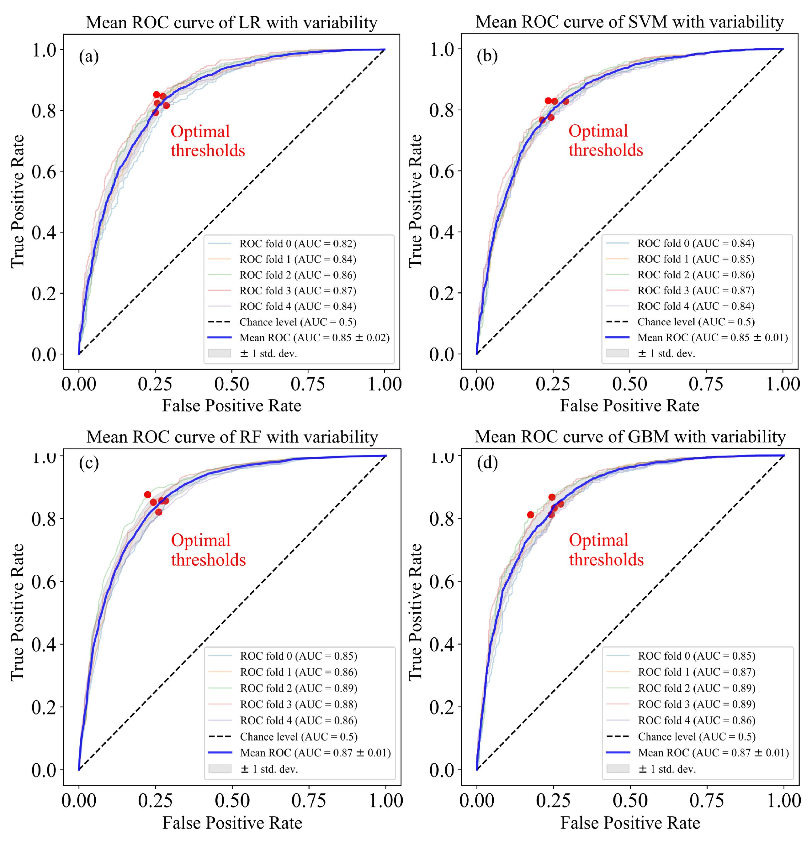
Table 2 shows the average model performance of the four algorithms with five-fold cross-validation. Hyperparameter tuning was conducted for each model to select the best set of hyperparameters that optimized the model’s performance. Among the four models, the GBM model yielded the highest AUC score of 0.871, which indicates a good performance in classifying landslides and non-landslides. By using five-fold cross-validation, five models are generated using data of different folds and the performance is evaluated using the remaining fold. Therefore, it is important to analyze the variance of the five models’ performance with cross-validation as it gives a better indication of how the model generalizes to an independent dataset. Figure 4 shows each model’s ROC curve and AUC score using different folds. For example, the mean AUC score of the five folds is 0.85 with a standard deviation of 0.02 when adopting the LR model. The ROC curve demonstrates the model performance at different probability thresholds, visualizing the trade-off between a model’s sensitivity and specificity. Hence, the optimal probability threshold is based on the point on the ROC curve that maximizes the TPR while minimizing the FPR. The optimal probability threshold for each model using different folds is shown as red dots in Figure 4.
A static LSM for the study area, as shown in Figure 5a, is generated using the optimal GBM model. According to the probability of landslide occurrence from 0 to 1, five susceptibility zones are classified with an equal interval of probability. The susceptibility zones of very low, low, moderate, high, and very high correspond to the probability of 0–20%, 20–40%, 40–60%, 60–80%, and 80–100%, respectively. It is found that most historical landslide data points are distributed within the areas of high and very high susceptibility on the map, which shows that the spatial LSM successfully captures the historical landslide distribution in the study area.
ML models are often referred to as black boxes, and one of the downsides of ML methods is the lack of ability to quickly interpret the results and explain the relationships between causative factors and predicted outcomes. One of the techniques that can be used to explain the contribution of input variables to model output is the SHapley Additive exPlanations (SHAP) method. The SHAP method is based on the cooperative game theory and can be used to increase the transparency and interpretability of ML models. A SHAP summary plot is generated to show how much a single feature affects the prediction. As shown in Figure 5b, the contour color turns red as the feature value increases; a higher SHAP value corresponds to a feature that steers the ML model toward a more positive prediction (i.e., a higher susceptibility of landslide); and the features are ranked based on their relative contribution to the model output and, from top to bottom, the feature becomes less important. The result shows that the prediction is consistent with geotechnical domain knowledge. For example, the slope parameter makes the most significant contribution to the output, and as the slope value increases, the model predicts a higher susceptibility to landslide occurrence. It should be noted that the trends shown in SHAP plots are specific to the dataset considered and may not be generalizable to other datasets.

5. ML for Spatiotemporal LSM

5.1. Spatiotemporal Landslide Sampling Method

Conventional LSM predicts the spatial distribution of landslide susceptibility by considering static causative factors that vary in space, such as topography, geology, hydro-meteorology, and land cover. However, pure spatial features cannot represent the timing of landslide occurrence at a given location. Non-landslides are sampled both in space and time to develop LSM for spatiotemporal prediction.
A landslide window period (LWP) is introduced for temporal sampling. As a type of natural hazard induced by climate events, rainfall-induced landslide activity is distinctly seasonal [45]. In this study, an LWP of 0.5 years was chosen based on landslide seasonality. Figure 6 shows the distribution of landslides in each month in the database. The typical landslide seasonality of 0.5 years is reflected through the offset from the peak landslide density to the minimum landslide density period. On the other hand, an LWP of integer years (i.e., 1 year, 2 years, etc.) represents sampling under similar climatic conditions. The precipitation profile triggering landslides is assumed to be unique in this study. Therefore, the data were also augmented temporally in integer years, allowing the ML models to learn the nuances between landslide and non-landslide occurrences under similar seasons.
Accurate landslide susceptibility prediction depends on reliable inventories, which necessitate extensive fieldwork or remote sensing efforts. However, many inventories are not regularly updated, potentially missing the impacts of environmental changes on landslide occurrence. Inventories derived from citizen reports of landslide occurrences have the potential to address these limitations [46]. In this study, landslide data were collected from multiple reliable sources. PennDOT conducts regular surveys to document the locations and dates of landslide events throughout Pennsylvania. The database from the NASA COOLR project is updated regularly and in a timely manner, collecting rainfall-triggered landslide events reported in the media, disaster databases, scientific reports, or other sources [26]. Therefore, these sources collectively represent the best available knowledge of landslide occurrences in the study area. Based on the comprehensive nature of these datasets, we assumed that the landslide data used in this study are representative of the true spatial and temporal distribution of landslides. Nevertheless, the proposed methods in this study can be improved with more reliable and complete data, which will be considered in future research.
Figure 7 shows the spatiotemporal sampling using an LWP of 1 year as an example. For each landslide on its event date, a non-landslide on the same date is randomly sampled within a ring-shaped buffer between 0.5 km and 1.5 km from the landslide location for spatial sampling. The size of the ring-shaped buffer zone accounts for the typical landslide sizes in the study area; the minimum distance of 0.5 km ensures that non-landslides randomly sampled in space will not coincide with the landslides, while the maximum distance of 1.5 km restricts the sampling range of non-landslides to avoid significant deviation of the input space. After spatial sampling, temporal sampling is conducted subsequently for both landslide samples and non-landslide samples. It is assumed that there was no landslide one year before the landslide date (given that no landslide was reported at the location one year prior). As such, for each landslide in the database, three corresponding non-landslides are created for an LWP of 1 year: one from spatial sampling and two from temporal sampling. Moreover, every sample in the spatiotemporal database is attached with both topographic and antecedent precipitation factors.
The data augmentation of non-landslides along spatial and temporal dimensions results in an imbalance in the number of positive and negative labels. The under-sampling method is applied in the study as it randomly selects negative samples with the same number of positive samples to form a balanced database for training ML models. Since under-sampled negative labels are chosen randomly, they can represent the original input distribution of augmented negative samples.

5.2. Results of Spatiotemporal ML

5.2.1. ML Results

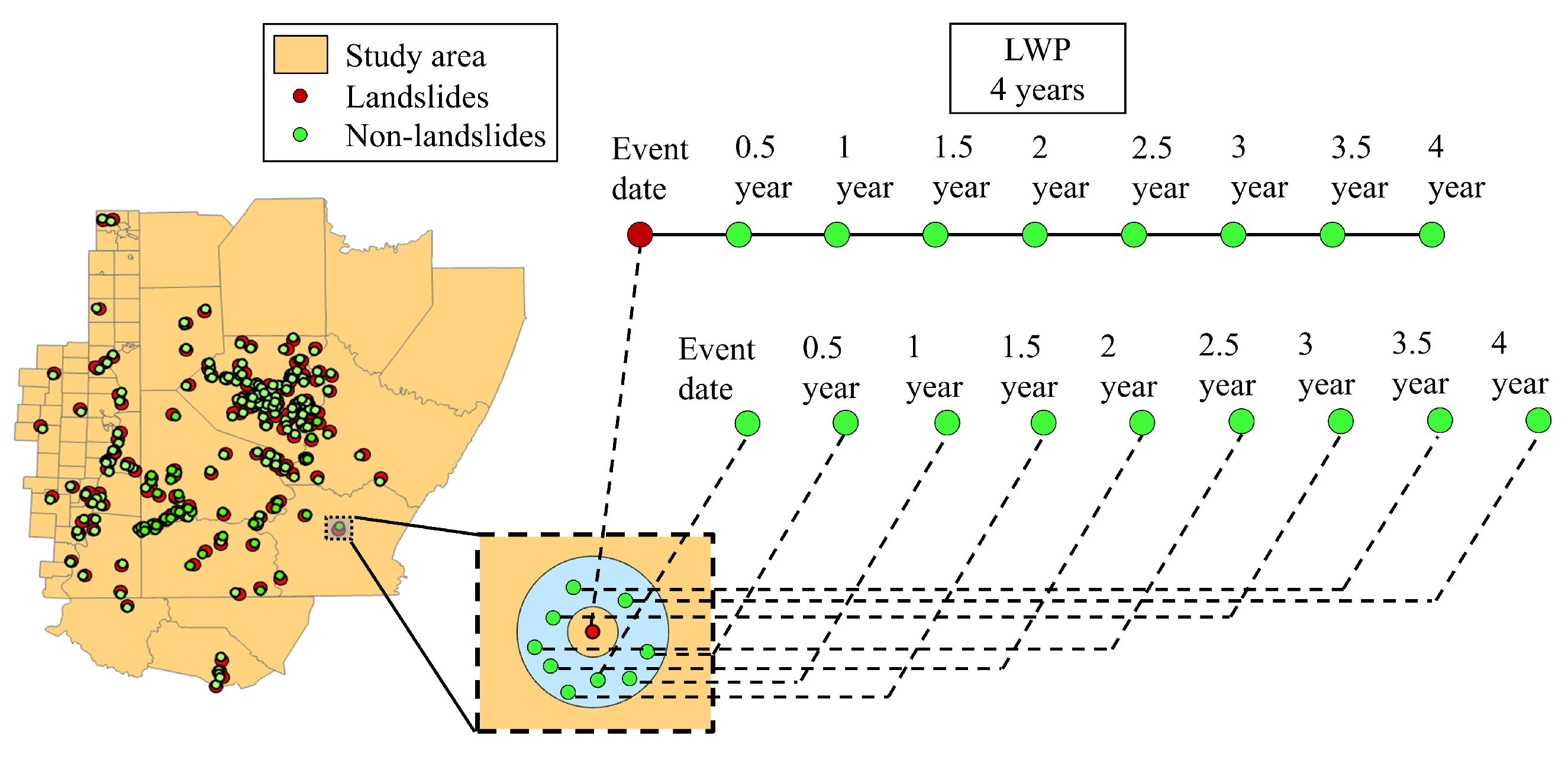
As different LWPs are considered, more non-landslide samples can be augmented into the spatiotemporal dataset through spatiotemporal sampling. Figure 8 shows the ways of data augmentation through both space and time by introducing non-landslides with different LWPs. From spatiotemporal dataset #1 to dataset #8, eight datasets were developed considering LWPs of up to four years with an interval of 0.5 years.
The number of temporal non-landslides is augmented as more LWPs are included. In the spatiotemporal dataset #8 shown in Figure 9, eight LWPs are used from 0.5 years to 4 years; for each landslide site, it is considered that there is no landslide occurrence 0.5 years, 1 year, 1.5 years, 2 years, 2.5 years, 3 years, 3.5 years, and 4 years prior to the event date at the same location. Each of the nine spatial non-landslides in the buffer zone is sampled in time with a specific LWP. The performance of ML models based on different spatiotemporal datasets is compared and analyzed. The results show that the RF algorithm outperforms the other three algorithms for all datasets.
The performance of the RF model for each dataset is shown in Table 3. It shows that model performance improves as more non-landslides are included in the spatiotemporal datasets. From datasets #1 to #7, as more non-landslide samples are augmented, the amount of spatiotemporal information introduced into the datasets increases. Hence, the ML models keep learning more representative and generalizable relationships to steadily improve the model performance. Table 3 shows that the AUC score reaches an optimum of 0.86 in the spatiotemporal dataset #7, where eight non-landslides are sampled in space, and seven LWPs are considered. However, as more spatiotemporal samples are included, the weights of newly added non-landslide samples are diluted because of the under-sampling method. Therefore, the model performance reaches an optimum when the effective spatiotemporal information in the dataset is saturated, as the results of datasets #7 and #8 indicate; dataset #8 is used as the final spatiotemporal landslide dataset to conduct spatiotemporal LSM.
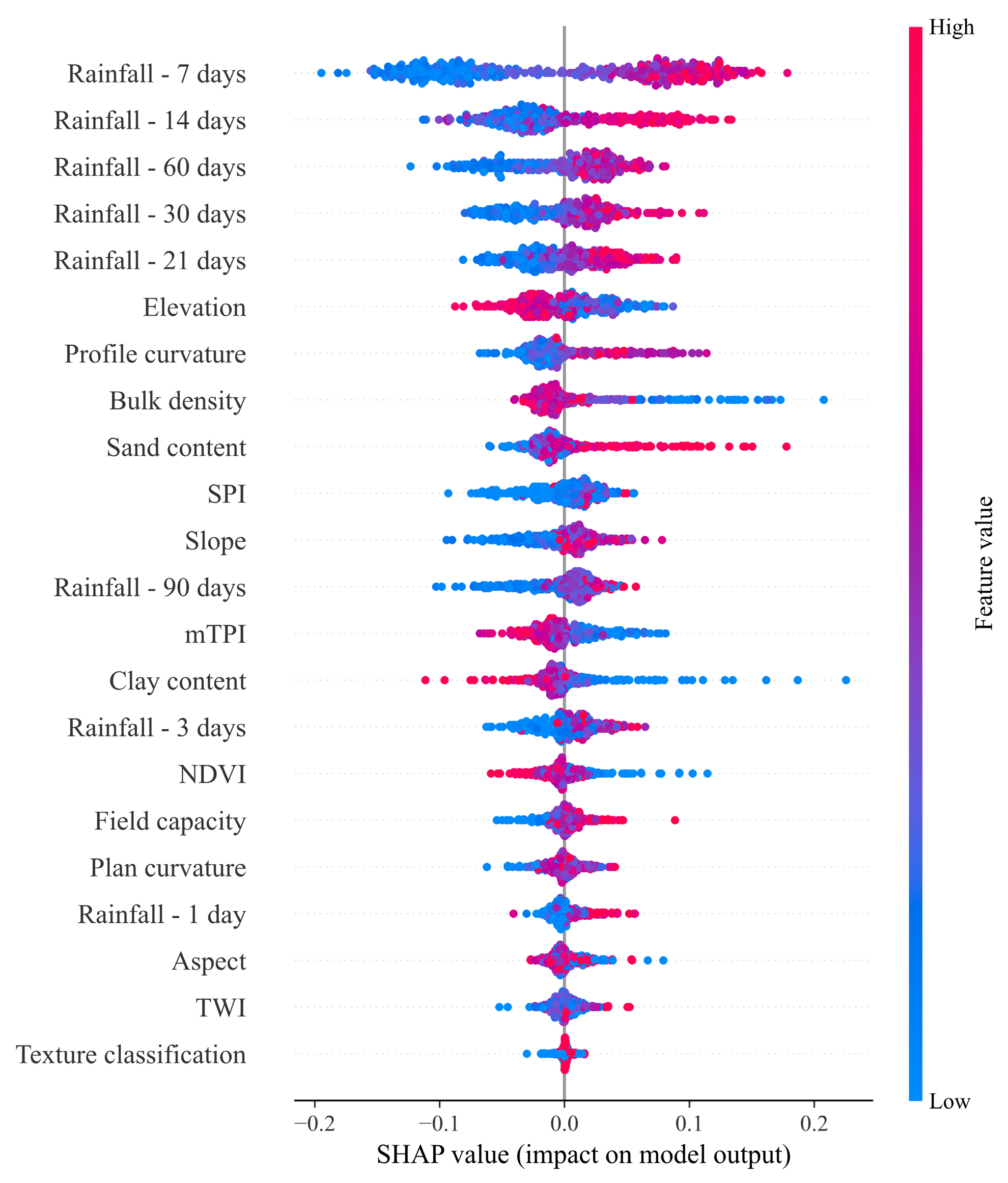
The feature importance in Figure 10 shows that the spatiotemporal ML model considers both the impact of spatial and temporal causative factors. Figure 10 shows that the 7-day cumulative precipitation preceding the landslide event is the most important factor for landslide occurrence, as the 7-day cumulative precipitation reflects the increase in soil saturation caused by rainfall and accounts for the lag effect. Besides the significant impact of rainfall factors, elevation, profile curvature, bulk density, and other topographic factors also contribute to the model outcome according to the SHAP plot, which reveals the hybridization of both spatial and temporal information in the developed model. The cumulative precipitation of various periods has a great effect on the potential of landslides for the dataset considered; this is consistent with geotechnical engineering experience in the study area that poor drainage conditions and lack of drainage maintenance during and after rainfall events contribute to landslide occurrence.

5.2.2. Spatiotemporal LSM

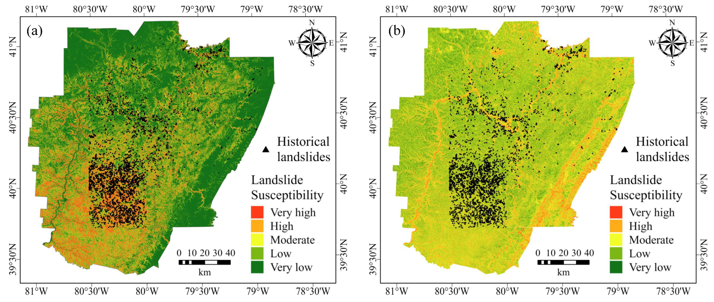
A conventional spatial LSM can also be developed using the spatiotemporal dataset with temporal information being disabled. A comparison of the spatial LSMs using different datasets is shown in Figure 11.
The ML model trained using spatial landslide inventory with 4543 samples demonstrates superior performance as the generated LSM can delineate areas with different susceptibility. However, in the spatial LSM based on a smaller spatiotemporal dataset with 223 landslide data points, there are large areas with low susceptibility to landslides but numerous actual landslide occurrences. The AUC scores for the model trained using spatial and spatiotemporal datasets are 0.87 and 0.77, respectively, further confirming the superior performance of the former model. This comparison shows the importance of the amount of training data in conducting conventional LSM with ML techniques.
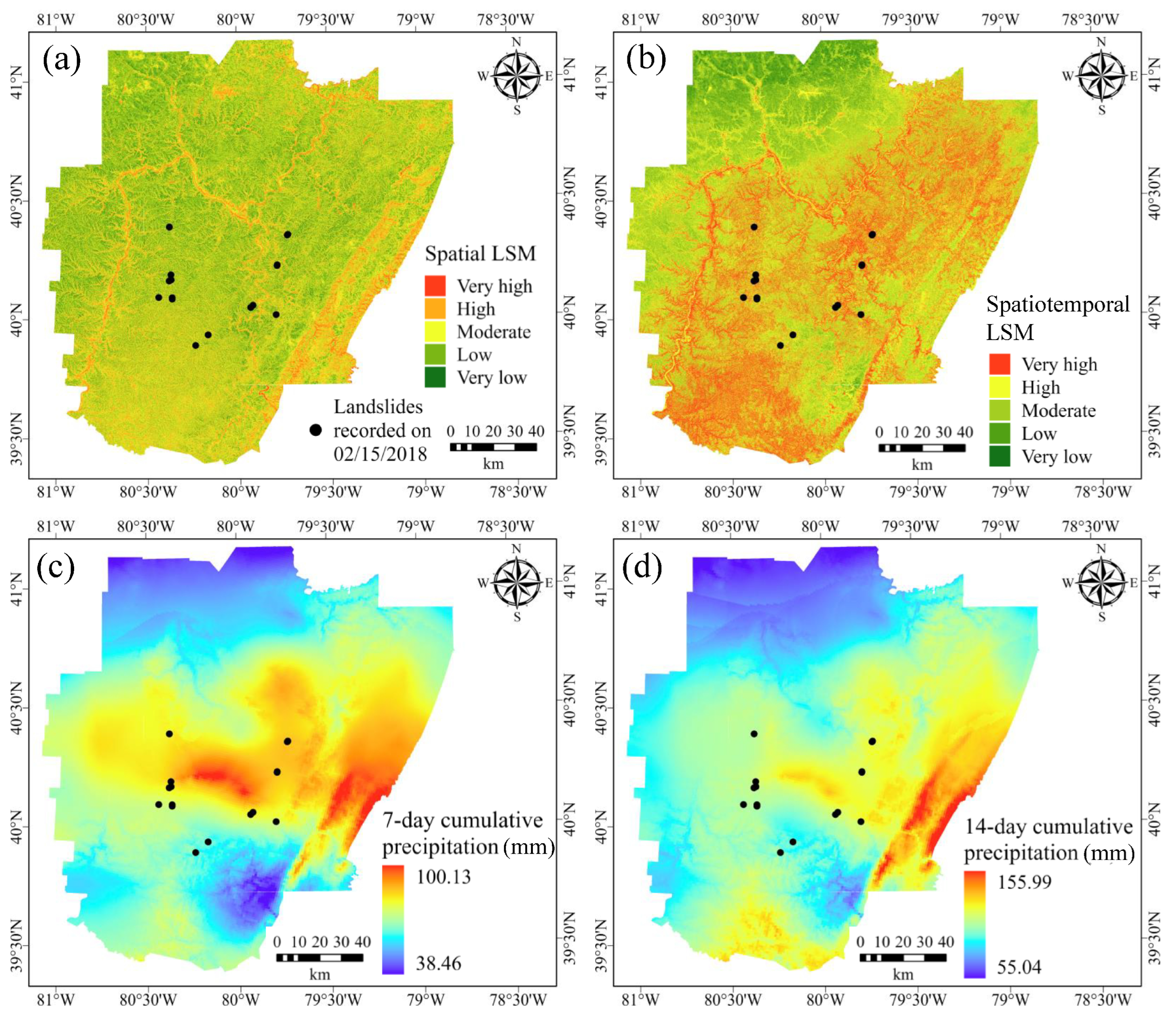
The conventional spatial LSM based on 223 landslide samples as the baseline model is also compared with spatiotemporal LSM. Figure 12 compares the performance of spatial and spatiotemporal LSMs for a storm event on 15 February 2018 when 17 landslide events were triggered and reported by PennDOT Districts 11 and 12. Table 4 shows the predicted susceptibilities from the two different LSMs for these landslides on 15 February 2018. The conventional spatial prediction shows a low probability (≤0.5) of landslide occurrence for some reported events; hence, considering only spatial causative factors, landslide susceptibility is significantly underestimated through LSM. On the other hand, by incorporating precipitation factors, the spatiotemporal LSM predicted much higher susceptibility at the locations of these landslides, consistent with their actual occurrence. Overall, the spatial distribution of the reported landslides on 15 February 2018 is much better matched with the spatiotemporal LSM than with the conventional spatial LSM. Figure 12c,d show the contours of cumulative precipitations of 7 days and 14 days before the event in the region, as the ML model indicates that these two rainfall factors contribute the most in spatiotemporal prediction (see Figure 10). Figure 12 shows that the spatiotemporal LSM accounts for the combined effects of topographic factors, as demonstrated in Figure 12a, and precipitation factors as demonstrated in Figure 12c,d.
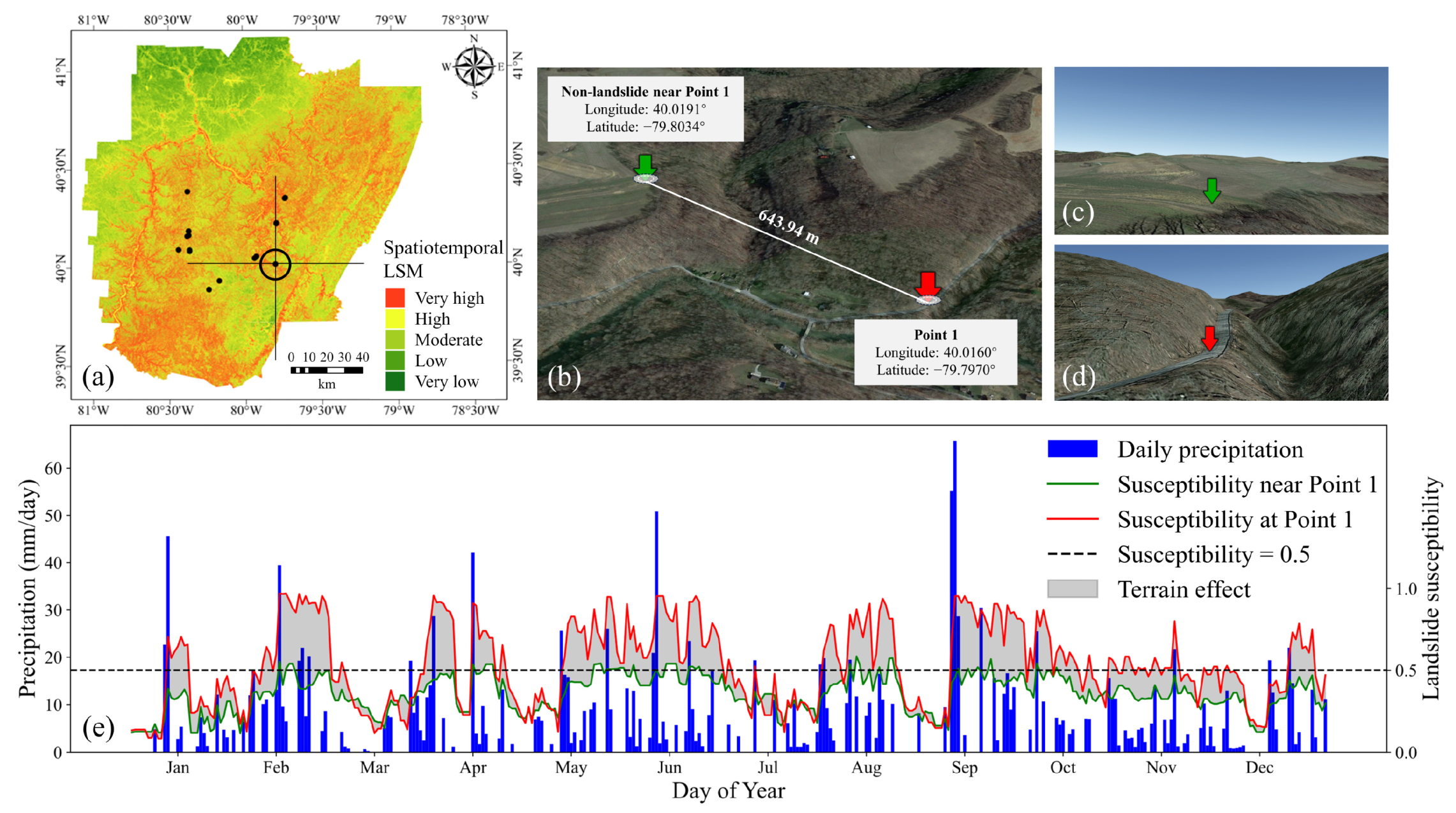
Due to the integration of temporal information, the spatiotemporal LSM dynamically varies with time based on precipitation data. As an example, Figure 13 shows the predicted susceptibility over time in 2018 at landslide point 1 (occurred on 15 February 2018) and an adjacent non-landslide point, and daily precipitation over the year. The distance between the two points is 644 m, which is smaller than the spatial resolution of rainfall data; hence, they have the same rainfall factors. The results show that the susceptibilities of both points follow the trend of daily precipitation with an evident lag influenced by the cumulation of precipitation. Under the same precipitation conditions, the difference between the susceptibility of the two sites is due to terrain factors. With a higher elevation and smaller slope angle, the non-landslide site has a relatively lower susceptibility than point 1. The typical trend of susceptibility over time and the terrain effect accounting for the susceptibility difference attest that the proposed spatiotemporal ML model integrates both temporal and spatial information to assess landslide susceptibility.

5.3. Computational Efficiency of Spatiotemporal LSM Application

The trend of using time-series DL models to predict temporal events has been gaining momentum due to their ability to capture complex temporal patterns. For example, Nava et al. [23] assessed and compared various DL models including LSTM, GRU, and a convolutional neural network (CNN) to forecast landslide temporal displacement across selected sites and highlighted the potential of DL models in landslide early warning systems. Zhao et al. [47] introduced a new model of evolutionary attention-based LSTM for predicting landslide displacement. The proposed model provided higher precision and interpretability in landslide prediction.
Time-series models like LSTM and GRU are particularly effective in forecasting landslide temporal occurrence by analyzing historical data on rainfall, soil moisture, and ground movement. However, they can be computationally intensive due to their complex architecture, which includes multiple gates (input, forget, and output gates) that require significant computational resources [48]. In addition, these models are designed to handle sequential data, where each data point depends on previous ones. This requires maintaining and updating hidden states across time steps, which increases computational complexity [49]. Therefore, time-series DL models require substantial memory and processing power, especially when dealing with large datasets or long sequences. Training those models can be time-consuming and may necessitate the use of GPUs to accelerate the process. In contrast, the spatiotemporal LSM approach in this study is model-agnostic, as tabular data are involved in the training process and sequential data are not necessarily required. The novelty of this approach lies in transforming rainfall time-series data into rainfall indices, which are commonly used for rainfall threshold analysis to evaluate landslide occurrences [50]. Hence, based on conventional ML algorithms, which are generally more computationally efficient compared to DL models as they have simpler architectures, lower computational demands are required for training and inference, and processing speed is faster, making them suitable for applications with limited computational resources.
In the application of spatiotemporal LSM, landslide causative factors and rainfall data can be downloaded in real-time. As more data are fed into the model, it can be continuously retrained and updated to achieve a more robust model, providing a more effective and reliable reference to landslide susceptibility.

6. Conclusions

Landslide susceptibility mapping over space has seen increasing attention in the last decade. While the current research mainly focuses on the spatial distribution of landslide risk, temporal landslide susceptibility assessments consider changes in causative factors over time, allowing us to understand how landslide susceptibility evolves. On the other hand, the paucity of a multi-temporal landslide inventory makes it unsuitable to apply time series prediction using deep learning. In this study, spatiotemporal LSM is conducted using conventional ML techniques to develop predictive models for landslides both on spatial and temporal scales. Two landslide databases in southwestern Pennsylvania and adjacent areas, containing 4543 and 223 historical landslide events for spatial analysis and spatiotemporal analysis, respectively, are compiled.
With fourteen topographic causative factors, the conventional LSM using spatial landslide inventory yields an AUC score of 0.87, showing a good consistency between historical landslide distribution and predicted susceptibility. However, the spatial LSM lacks the ability to represent landslide temporal distribution. Based on the spatiotemporal landslide inventory, and with eight antecedent cumulative precipitation factors included as temporal features, the spatiotemporal LSM is carried out to predict landslide occurrence both in space and time. Despite insufficient training data, novel data augmentation is applied through non-landslide sampling both in space and time based on domain knowledge to incorporate spatiotemporal information into the datasets. Different spatiotemporal landslide datasets are developed as non-landslides with different window periods. The optimal spatiotemporal ML model achieves an AUC score of 0.86, which outperforms the conventional spatial model with the same quantity of training data. As the feature contributions and results of landslide susceptibility over time show, the proposed model hybridizes the information from both spatial terrain factors and temporal rainfall factors, showing good model explainability. Therefore, an alternative method to develop LSM for both spatial and temporal prediction is provided in this study, which shows the potential for applications in landslide hazard mitigation and forecasting due to its simplicity, effectiveness, and applicability with small datasets.

Author Contributions

Conceptualization, J.X., T.P. and T.Q.; Formal analysis, J.X.; Data curation, J.X.; Writing—original draft, J.X.; Writing—review & editing, T.P. and T.Q.; Supervision, T.Q. All authors have read and agreed to the published version of the manuscript.

Funding

This research was funded by the Pennsylvania Department of Transportation under PSUCIAMTIS2019 WO 002. The APC was funded by the University of Utah.

Data Availability Statement

All data sources are described in the article. Some data, models, or codes that support the findings of this study are available from the corresponding author upon reasonable request. These data include the results used to generate all figures and tables.

Conflicts of Interest

The authors declare no conflicts of interest.

References

  1. Wei, X.; Zhang, L.; Luo, J.; Liu, D. A hybrid framework integrating physical model and convolutional neural network for regional landslide susceptibility mapping. Nat. Hazards 2021, 109, 471–497. [Google Scholar] [CrossRef]
  2. Xing, Y.; Yue, J.; Guo, Z.; Chen, Y.; Hu, J.; Travé, A. Large-scale landslide susceptibility mapping using an integrated machine learning model: A case study in the Lvliang Mountains of China. Front. Earth Sci. 2021, 9, 622. [Google Scholar] [CrossRef]
  3. Pei, T.; Qiu, T. Landslide susceptibility mapping using physics-guided machine learning: A case study of a debris flow event in Colorado Front Range. Acta Geotech. 2024; in press. [Google Scholar] [CrossRef]
  4. Pei, T.; Qiu, T. Landslide Susceptibility Mapping Using Machine Learning Methods: A Case Study in Colorado Front Range, USA. Geo-Congress 2023, 2023, 521–530. [Google Scholar] [CrossRef]
  5. Pei, T.; Qiu, T. Debris flow susceptibility mapping in Colorado Front Range, USA: A comparison of physics-based and data-driven approaches. In Proceedings of the 8th International Conference on Debris Flow Hazard Mitigation (DFHM8), Torino, Italy, 26–29 June 2023. E3S Web of Conferences. [Google Scholar] [CrossRef]
  6. Yesilnacar, E.; Topal, T. Landslide susceptibility mapping: A comparison of logistic regression and neural networks methods in a medium scale study, Hendek region (Turkey). Eng. Geol. 2005, 79, 251–266. [Google Scholar] [CrossRef]
  7. Chacon, J.; Irigaray, C.; Fernandez, T.; El-Hamdouni, R. Engineering geology maps: Landslides and geographical information systems. Bull. Eng. Geol. Environ. 2006, 65, 341–411. [Google Scholar] [CrossRef]
  8. Lee, S.; Pradhan, B. Landslide hazard mapping at Selangor, Malaysia using frequency ratio and logistic regression models. Landslides 2007, 4, 33–41. [Google Scholar] [CrossRef]
  9. Yilmaz, I. Comparison of landslide susceptibility mapping methodologies for Koyulhisar, Turkey: Conditional probability, logistic regression, artificial neural networks, and support vector machine. Environ. Earth Sci. 2010, 61, 821–836. [Google Scholar] [CrossRef]
  10. Akgun, A. A comparison of landslide susceptibility maps produced by logistic regression, multi-criteria decision, and likelihood ratio methods: A case study at İzmir, Turkey. Landslides 2012, 9, 93–106. [Google Scholar] [CrossRef]
  11. Youssef, A.M. Landslide susceptibility delineation in the Ar-Rayth area, Jizan, Kingdom of Saudi Arabia, using analytical hierarchy process, frequency ratio, and logistic regression models. Environ. Earth Sci. 2015, 73, 8499–8518. [Google Scholar] [CrossRef]
  12. Wang, Y.; Song, C.; Lin, Q.; Li, J. Occurrence probability assessment of earthquake-triggered landslides with Newmark displacement values and logistic regression: The Wenchuan earthquake, China. Geomorphology 2016, 258, 108–119. [Google Scholar] [CrossRef]
  13. Corominas, J.; Van Westen, C.; Frattini, P.; Cascini, L.; Malet, J.P.; Fotopoulou, S.; Catani, F.; Van Den Eeckhaut, M.; Mavrouli, O.; Agliardi, F.; et al. Recommendations for the quantitative analysis of landslide risk. Bull. Eng. Geol. Environ. 2014, 73, 209–263. [Google Scholar] [CrossRef]
  14. Xiong, J.; Pei, T.; Qiu, T. Spatiotemporal Prediction of Rainfall-induced Landslides Using Machine Learning Techniques. In IOP Conference Series: Earth and Environmental Science; IOP Publishing: Bristol, UK, 2024; Volume 1337. [Google Scholar]
  15. Reichenbach, P.; Rossi, M.; Malamud, B.D.; Mihir, M.; Guzzetti, F. A review of statistically-based landslide susceptibility models. Earth Sci. Rev. 2018, 180, 60–91. [Google Scholar] [CrossRef]
  16. Huang, Y.; Zhao, L. Review on landslide susceptibility mapping using support vector machines. Catena 2018, 165, 520–529. [Google Scholar] [CrossRef]
  17. Merghadi, A.; Yunus, A.P.; Dou, J.; Whiteley, J.; ThaiPham, B.; Bui, D.T.; Avtar, R.; Abderrahmane, B. Machine learning methods for landslide susceptibility studies: A comparative overview of algorithm performance. Earth-Sci. Rev. 2020, 207, 103225. [Google Scholar] [CrossRef]
  18. Moziihrii, A.; Khwairakpam, A.; Arnab, K.M.; Elzbieta, J.; Radomir, G.; Zbigniew, L.; Michał, J. Landslide Susceptibility Mapping Using Machine Learning: A Literature Survey. Remote Sens. 2022, 14, 3029. [Google Scholar] [CrossRef]
  19. Rosi, A.; Peternel, T.; Jemec-Auflič, M.; Komac, M.; Segoni, S.; Casagli, N. Rainfall thresholds for rainfall-induced landslides in Slovenia. Landslides 2016, 13, 1571–1577. [Google Scholar] [CrossRef]
  20. Peruccacci, S.; Brunetti, M.T.; Gariano, S.L.; Melillo, M.; Rossi, M.; Guzzetti, F. Rainfall thresholds for possible landslide occurrence in Italy. Geomorphology 2017, 290, 39–57. [Google Scholar] [CrossRef]
  21. Huang, F.; Chen, J.; Liu, W.; Huang, J.; Hong, H.; Chen, W. Regional rainfall-induced landslide hazard warning based on landslide susceptibility mapping and a critical rainfall threshold. Geomorphology 2022, 408, 108236. [Google Scholar] [CrossRef]
  22. Khalili, M.A.; Guerriero, L.; Pouralizadeh, M.; Calcaterra, D.; Martire, D.D. Monitoring and prediction of landslide-related deformation based on the GCN-LSTM algorithm and SAR imagery. Nat. Hazards 2023, 119, 39–68. [Google Scholar] [CrossRef]
  23. Nava, L.; Carraro, E.; Reyes-Carmona, C.; Puliero, S.; Bhuyan, K.; Rosi, A.; Monserrat, O.; Floris, M.; Meena, S.R.; Galve, J.P.; et al. Landslide displacement forecasting using deep learning and monitoring data across selected sites. Landslides 2023, 20, 2111–2129. [Google Scholar] [CrossRef]
  24. Delano, H.L.; Wilshusen, J.P. Landslides in Pennsylvania (2nd ed.): Pennsylvania Geological Survey, 4th ser., Educational Series 9, 2001, 34p. Available online: https://maps.dcnr.pa.gov/publications/Default.aspx?id=272 (accessed on 2 September 2024).
  25. Pomeroy, J.S.; William, E.D. Landslides and Related Features, Pennsylvania-Pittsburgh 1° × 2° Sheet; US Geological Survey: Reston, VA, USA, 1979. [Google Scholar] [CrossRef]
  26. Kirschbaum, D.B.; Adler, R.; Hong, Y.; Hill, S.; Lerner-Lam, A. A global landslide catalog for hazard applications: Method, results, and limitations. Nat. Hazards 2010, 52, 561–575. [Google Scholar] [CrossRef]
  27. Kirschbaum, D.B.; Stanley, T.; Zhou, Y. Spatial and Temporal Analysis of a Global Landslide Catalog. Geomorphology 2015, 249, 4–15. [Google Scholar] [CrossRef]
  28. Kavzoglu, T.; Colkesen, I.; Sahin, E.K. Machine learning techniques in landslide susceptibility mapping: A survey and a case study. In Landslides: Theory, Practice and Modelling; Springer: Berlin/Heidelberg, Germany, 2019; pp. 283–301. [Google Scholar]
  29. Beyabanaki, S.A.R.; Bagtzoglou, A.C.; Anagnostou, E.N. Effects of groundwater table position, soil strength properties and rainfall on instability of earthquake-triggered landslides. Environ. Earth Sci. 2016, 75, 358. [Google Scholar] [CrossRef]
  30. Zhang, M.; Singh, H.V.; Migliaccio, K.W.; Kisekka, I. Evaluating water table response to rainfall events in a shallow aquifer and canal system. Hydrol. Process. 2017, 31, 3907–3919. [Google Scholar] [CrossRef]
  31. Crozier, M.J. Landslides: Causes, Consequences and Environment; Croom Helm: Beckenham, UK, 1986; pp. 171–192. [Google Scholar]
  32. Patton, A.I.; Luna, L.V.; Roering, J.J.; Jacobs, A.; Korup, O.; Mirus, B.B. Landslide initiation thresholds in data-sparse regions: Application to landslide early warning criteria in Sitka, Alaska, USA. Nat. Hazards Earth Syst. Sci. 2023, 23, 3261–3284. [Google Scholar] [CrossRef]
  33. Nolasco-Javier, D.; Kumar, L. Deriving the rainfall threshold for shallow landslide early warning during tropical cyclones: A case study in northern Philippines. Nat. Hazards 2018, 90, 921–941. [Google Scholar] [CrossRef]
  34. Kim, S.W.; Chun, K.W.; Kim, M.; Catani, F.; Choi, B.; Seo, J. Effect of antecedent rainfall conditions and their variations on shallow landslide-triggering rainfall thresholds in South Korea. Landslides 2021, 18, 569–582. [Google Scholar] [CrossRef]
  35. Guzzetti, F.; Peruccacci, S.; Rossi, M.; Stark, C.P. Rainfall thresholds for the initiation of landslides in central and southern Europe. Meteorol. Atmos. Phys 2007, 98, 239–267. [Google Scholar] [CrossRef]
  36. Vapnik, V.N. The Nature of Statistical Learning Theory; Springer: New York, NY, USA, 1995. [Google Scholar]
  37. Ho, T.K. Random decision forests. In Proceedings of the 3rd International Conference on Document Analysis and Recognition, Montreal, QC, Canada, 14–16 August 1995; Volume 1, pp. 278–282. [Google Scholar]
  38. Natekin, A.; Knoll, A. Gradient boosting machines, a tutorial. Front. Neurorobot. 2013, 7, 21. [Google Scholar] [CrossRef]
  39. Ayalew, L.; Yamagishi, H. The application of GIS-based logistic regression for landslide susceptibility mapping in the Kakuda-Yahiko Mountains, Central Japan. Geomorphology 2005, 65, 15–31. [Google Scholar] [CrossRef]
  40. Ballabio, C.; Sterlacchini, S. Support Vector Machines for Landslide Susceptibility Mapping: The Staffora River Basin Case Study, Italy. Math Geosci. 2012, 44, 47–70. [Google Scholar] [CrossRef]
  41. Zhang, W.; He, Y.; Wang, L.; Liu, S.; Meng, X. Landslide Susceptibility mapping using random forest and extreme gradient boosting: A case study of Fengjie, Chongqing. Geol. J. 2023, 58, 2372–2387. [Google Scholar] [CrossRef]
  42. Akosah, S.; Gratchev, I.; Kim, D.-H.; Ohn, S.-Y. Application of Artificial Intelligence and Remote Sensing for Landslide Detection and Prediction: Systematic Review. Remote Sens. 2024, 16, 2947. [Google Scholar] [CrossRef]
  43. Huang, F.; Cao, Y.; Li, W.; Catani, F.; Song, G.; Huang, J.; Yu, C. Uncertainties of landslide susceptibility prediction: Influences of different study area scales and mapping unit scales. Int. J. Coal. Sci. Technol. 2024, 11, 26. [Google Scholar] [CrossRef]
  44. Woodard, J.B.; Mirus, B.B.; Crawford, M.M.; Or, D.; Leshchinsky, B.A.; Allstadt, K.E.; Wood, N.J. Mapping landslide susceptibility over large regions with limited data. J. Geophys. Res. Earth Surf. 2023, 128, e2022JF006810. [Google Scholar] [CrossRef]
  45. Luna, L.V.; Korup, O. Seasonal Landslide Activity Lags Annual Precipitation Pattern in the Pacific Northwest. Geophys. Res. Lett. 2022, 49, e2022GL098506. [Google Scholar] [CrossRef]
  46. Rohan, T.J.; Wondolowski, N.; Shelef, E. Landslide susceptibility analysis based on citizen reports. Earth Surf. Process. Landf. 2021, 46, 791–803. [Google Scholar] [CrossRef]
  47. Zhao, Q.; Wang, H.; Zhou, H.; Gan, F.; Yao, L.; Zhou, Q.; An, Y. An interpretable and high-precision method for predicting landslide displacement using evolutionary attention mechanism. Nat. Hazards, 2024; in press. [Google Scholar] [CrossRef]
  48. Violos, J.; Psomakelis, E.; Danopoulos, D.; Tsanakas, S.; Varvarigou, T. Using LSTM Neural Networks as Resource Utilization Predictors: The Case of Training Deep Learning Models on the Edge. In Economics of Grids, Clouds, Systems, and Services; Springer: Cham, Switzerland, 2020; pp. 67–74. [Google Scholar] [CrossRef]
  49. Rahimzad, M.; Moghaddam Nia, A.; Zolfonoon, H.; Soltani, J.; Danandeh Mehr, A.; Kwon, H.H. Performance Comparison of an LSTM-based Deep Learning Model versus Conventional Machine Learning Algorithms for Streamflow Forecasting. Water Resour. Manag. 2021, 35, 4167–4187. [Google Scholar] [CrossRef]
  50. Segoni, S.; Piciullo, L.; Gariano, S.L. A review of the recent literature on rainfall thresholds for landslide occurrence. Landslides 2018, 15, 1483–1501. [Google Scholar] [CrossRef]
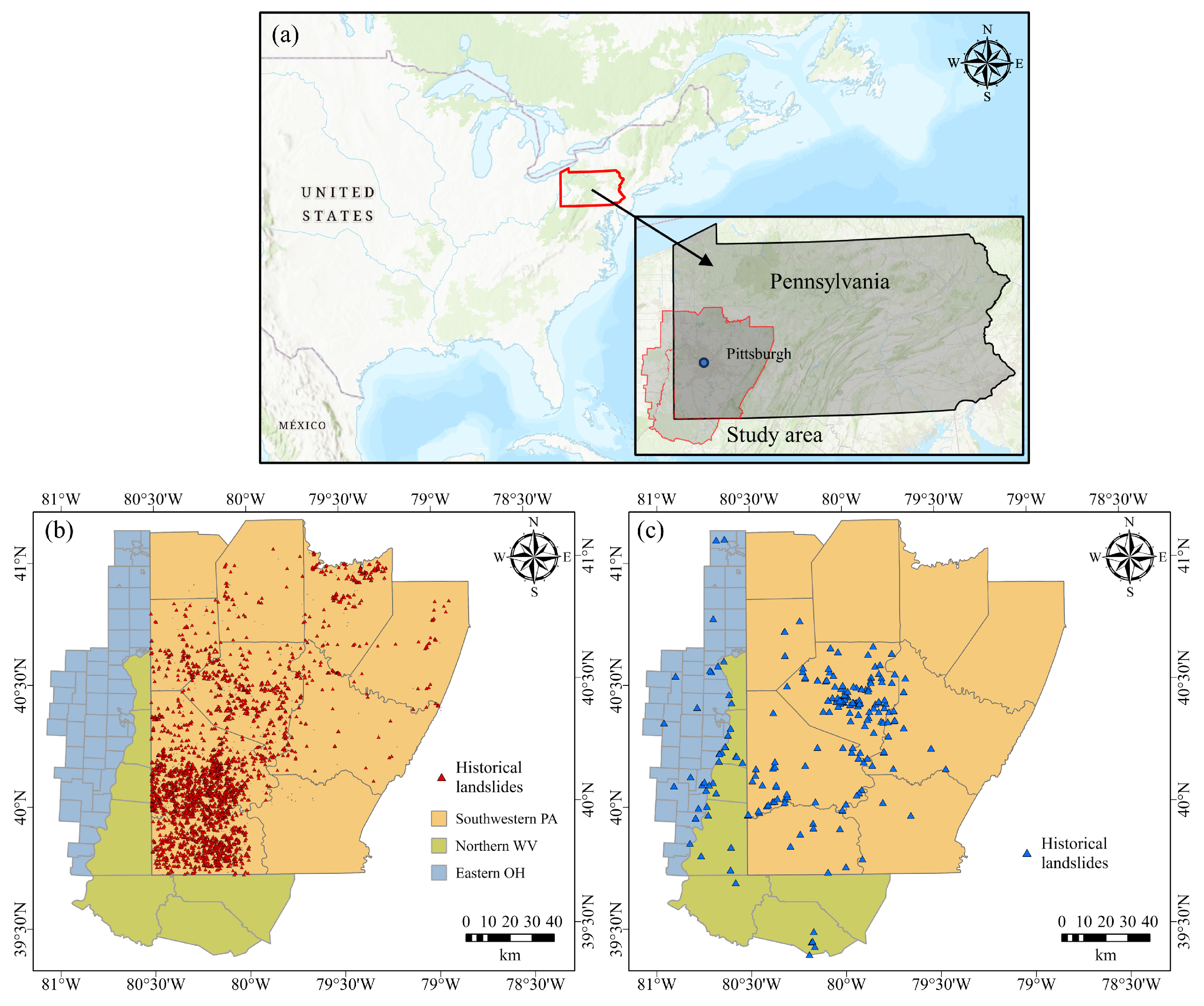
Figure 1. Maps of the study area: (a) location of the study area; (b) regional distribution of landslides in the spatial database; (c) regional distribution of landslides in the spatiotemporal database.
Remotesensing 16 03526 g001
Figure 2. Causative factors for LSM: (a) elevation; (b) slope; (c) aspect; (d) mTPI; (e) TWI; (f) SPI; (g) profile curvature; (h) plan curvature; (i) NDVI; (j) clay content; (k) sand content; (l) bulk density; (m) field capacity; (n) soil texture. (These data are publicly available from Google Earth Engine and can be downloaded at https://earthengine.google.com, accessed on 2 September 2024).
Remotesensing 16 03526 g002
Figure 3. Landslide and non-landslide samples in the study area.
Remotesensing 16 03526 g003
Figure 4. ROC curve and AUC score of different ML models: (a) LR; (b) SVM; (c) RF; (d) GBM.
Remotesensing 16 03526 g004
Figure 5. Results of spatial LSM using the GBM algorithm: (a) spatial LSM; (b) SHAP plot.
Remotesensing 16 03526 g005
Figure 6. Monthly distribution of landslides collected in the database.
Remotesensing 16 03526 g006
Figure 7. Sampling approach for spatiotemporal LSM.
Remotesensing 16 03526 g007
Figure 8. Spatiotemporal datasets with different non-landslide locations and LWPs.
Remotesensing 16 03526 g008
Figure 9. Spatiotemporal dataset #8 with the LWP of 4 years.
Remotesensing 16 03526 g009
Figure 10. SHAP plot for the spatiotemporal LSM model.
Remotesensing 16 03526 g010
Figure 11. Comparison of conventional spatial LSMs using different databases: (a) 4543 landslide samples; (b) 223 landslide samples.
Remotesensing 16 03526 g011
Figure 12. LSM and precipitation maps for 15 February 2018: (a) pure spatial LSM; (b) spatiotemporal LSM; (c) 7-day cumulative precipitation map; (d) 14-day cumulative precipitation map.
Remotesensing 16 03526 g012
Figure 13. Landslide susceptibility over time in 2018 at landslide point 1 (occurred on 15 February 2018) and an adjacent non-landslide point: (a) location of point 1; (b) spatial relationship between point 1 and non-landslide point; (c,d) terrain of point 1 and non-landslide point; (e) landslide susceptibility over time in 2018.
Remotesensing 16 03526 g013
Table 1. Causative factors used for LSM.
Causative FactorUnitData ResolutionData Source
Elevationm30 mNASADEM
Slopedeg
Aspectdeg
Multi-scale topographic position index (mTPI)m
Profile curvature-
Plan curvature-
Topographic wetness index (TWI)-
Stream power index (SPI)-
Normalized difference vegetation index (NDVI)-
Sand content%250 mOpenLandMap
Clay content%
Bulk density10 kg/m3
Texture classification-
Field capacity%
Table 2. Model performance using ML methods for spatial LSM.
ModelAccuracyPrecisionRecallF1AUCHyperparameters
LR0.7750.7630.8000.7800.847Slover: LBFGS; penalty: L1; C: 0.2
SVM0.7750.7550.8130.7830.850Kernel: RBF; C:10; gamma: 0.0001
RF0.7920.7770.8210.7980.868n_estimators: 80; min_samples_split: 2;
min_samples_leaf: 6; max_depth: 10
GBM0.7950.7750.8330.8020.871learning rate: 0.1; n_estimators: 50; min_samples_split: 2; min_samples_leaf: 1; max_depth: 3
Avg.0.7840.7680.8170.7910.859
Table 3. RF model performance for spatiotemporal LSM with different datasets.
Dataset NumberAccuracyPrecisionRecallF1 ScoreAUC Score
10.710.720.690.710.77
20.720.730.690.710.79
30.750.770.700.730.81
40.760.780.720.750.83
50.770.800.700.750.84
60.780.790.740.760.85
70.790.810.720.770.86
80.780.790.760.770.86
Table 4. Predicted susceptibilities from pure spatial and spatiotemporal models for the landslides on 15 February 2018.
Landslide
Point
LatitudeLongitudeSusceptibility
Pure Spatial
ML Model
Spatiotemporal
ML Model
1−79.7970°40.0160°0.620.97
2−80.2379°39.8897°0.740.86
3−80.1696°39.9339°0.210.83
4−79.9229°40.0566°0.850.99
5−79.9359°40.0472°0.510.76
6−80.4378°40.0925°0.510.86
7−80.3647°40.0857°0.310.79
8−80.3642°40.0916°0.580.87
9−80.3771°40.3887°0.630.91
10−80.3804°40.1618°0.740.88
11−80.3695°40.1664°0.470.67
12−80.3701°40.1877°0.590.82
13−79.7883°40.2222°0.800.90
14−79.7886°40.2226°0.730.93
15−79.7877°40.2255°0.840.97
16−79.7304°40.3505°0.700.99
17−79.7274°40.3529°0.740.94
Disclaimer/Publisher’s Note: The statements, opinions and data contained in all publications are solely those of the individual author(s) and contributor(s) and not of MDPI and/or the editor(s). MDPI and/or the editor(s) disclaim responsibility for any injury to people or property resulting from any ideas, methods, instructions or products referred to in the content.