Abstract
Meteorological satellite remote sensing is important for numerical weather forecasts, but its accuracy is affected by many things during observation and retrieval, showing that it can be improved. As a standard way to measure wind from space, atmospheric motion vectors (AMVs) are used. They are separate pieces of information spread out in the troposphere, which gives them more depth than regular surface or sea surface wind measurements. This makes rectifying problems more difficult. For error correction, this research builds a deep-learning model that is specific to AMVs. The outcomes show that AMV observational errors are greatly reduced after correction. The root mean square error (RMSE) drops by almost 40% compared to ERA5 true values. Among these, the optimization of solar observation errors exceeds 40%; the discrepancies at varying atmospheric pressure altitudes are notably improved; the degree of optimization for data with low QI coefficients is substantial; and there remains potential for enhancement in data with high QI coefficients. Furthermore, there has been a significant enhancement in the consistency coefficient of the wind’s physical properties. In the assimilation forecasting experiments, the corrected AMV data demonstrated superior forecasting performance. With more training, the model can fix things better, and the changes it makes last for a long time. The results show that it is possible and useful to use deep learning to fix errors in meteorological remote-sensing data.
1. Introduction
Numerical weather prediction (NWP) is a modern approach to meteorological forecasting that combines mathematical, physical, and computer science techniques to accurately and impartially predict upcoming weather patterns [1,2]. This intricate interdisciplinary system is widely recognized as a groundbreaking accomplishment in the field of physics [3]. The heart of NWP involves solving differential equations that describe atmospheric motion. This requires providing initial fields and boundary conditions. The accuracy of the initial fields has a direct impact on the overall prediction results. Advanced data-assimilation techniques enable the use of multiple data sources to refine initial field information, which is a key reason for significant improvements in NWP systems [4,5]. In order to ensure the accuracy of the initial fields, it is essential to have high-quality observational data.
Advancements in detection technologies have significantly expanded the availability of meteorological data sources, especially after the United States launched the world’s first meteorological satellite in 1960. Breakthroughs in satellite remote-sensing technology have introduced new methods for acquiring atmospheric information, greatly enriching meteorological data. Satellite data are among the most important observation sources for global numerical weather prediction, comprising over 90% of all data [6,7,8].
Compared to traditional observations, satellite remote sensing stands out for its exceptional resolution, consistent spatiotemporal coverage, and unrestricted observation capabilities. The observational elements include common variables such as temperature, pressure, wind fields, and humidity. Nevertheless, errors can arise in remote-sensing equipment and the retrieval process, leading to a need for enhanced accuracy in certain data. Atmospheric motion vectors (AMVs), typical satellite remote-sensing wind measurement data, estimate atmospheric wind fields by tracking cloud clusters in meteorological satellite images [9,10]. Wind fields are more complex than variables like temperature and pressure because they include both wind direction and wind speed components. Additionally, AMVs are discrete data distributed throughout the troposphere, adding a vertical dimension compared to conventional surface or sea surface wind measurements, presenting greater challenges for error correction.
AMVs play a crucial role in enhancing our understanding of atmospheric wind patterns, providing valuable data on upper-level wind fields. They can effectively improve the accuracy of typhoon intensity and path predictions and precipitation forecasts in numerical predictions [11,12,13]. This makes them valuable for error correction. There are two main sources of error when it comes to AMVs: inaccurate estimation of wind vectors and significant errors in height assignment [14]. Numerous researchers have conducted extensive studies on error correction for AMVs, particularly regarding height assignment issues. These include using infrared cloud imagery for height correction of AMVs [15], applying Feature Tracking Correction (FTC) to the AMV observation operator for height adjustment [16], and adjusting low-level AMV heights using numerical model cloud information [17]. Still, there is potential for enhancing the effectiveness of corrections. The complexity and uncertainty of the meteorological environment, along with the massive data accumulation from the exponential growth of meteorological data that has yet to be fully mined and utilized [18], necessitate more effective methods for error correction of meteorological remote-sensing data.
Artificial intelligence (AI) technology has been extensively utilized in meteorology and oceanography since the 1980s [19]. Its primary applications include identifying, classifying, and ensuring the quality of various observations, such as clouds, tornadoes, strong winds, hail, precipitation, and storms. Over the past few years, researchers have incorporated advanced AI technologies into meteorological and oceanographic forecasting. This includes utilizing infrared cloud images to identify and predict tropical cyclones, as well as detecting mesoscale eddies in the ocean [20,21,22]. AI technology can offer a “lightweight” method for higher precision forecasting, utilizing fewer computational resources [23]. It can address challenges in NWP related to initial values, physical processes, and error correction.
Deep learning, an essential component of AI technology, is commonly referred to as representation learning. With the continuous growth in data-acquisition capabilities and advances in hardware technology (such as high-performance GPUs), deep learning has led to new research in deep and distributed learning. Emerging from the realm of traditional machine learning has proven to be far superior to its predecessor. Utilizing transformation and graph technologies, this approach constructs multi-layer learning models that yield exceptional outcomes in audio and speech processing, visual data processing, and natural language processing [24,25,26,27]. Deep learning continuously improves model performance with increasing data scales, making it highly suitable for the ever-growing meteorological data. Scholars have made substantial contributions in this field. For instance, Tao et al. [28] utilized a deep neural network with radar echo and optical flow images to study intelligent identification of severe convective weather. Seok-Geun et al. [29] applied deep learning to nowcasting heavy precipitation, showing it can outperform numerical predictions in short-term forecasting of heavy precipitation. In their study, Wang et al. [30] created a deep-learning model that was able to detect tropical cyclones and make estimates about their radii using satellite infrared cloud images.
This study aims to improve the accuracy of initial fields in NWP and enhance forecasting performance. It focuses on addressing initial error issues in meteorological satellite remote-sensing data, specifically AMVs. These data present significant correction challenges and have high utilization values. This study explores the advantages of deep learning by constructing a network model for AMVs, effectively utilizing their deep spatiotemporal features for error correction, which were designed to minimize observational errors, resulting in more precise upper-level atmospheric wind field data. As a result, the accuracy of meteorological satellite remote-sensing data and overall forecasting performance can be significantly improved.
2. Data
2.1. AMV Data
Over the past few years, advancements in observation instruments and retrieval methods for AMVs have sparked a surge of research and experimentation conducted by many scholars. Otsuka et al. [31] analyzed the error characteristics of AMV data from Japan’s Himawari-8 satellite relative to the Japan Meteorological Agency (JMA) model background field. Velden et al. [32] utilized AMV data from geostationary meteorological satellites to conduct assimilation experiments aimed at predicting tropical cyclones. Kunii et al. [33] found that assimilating Himawari-8 satellite AMV data positively impacts rainfall forecast timing and intensity. Zhao Juan et al. [34] conducted assimilation experiments using AMV data from the GEOS-16 satellite. The results showed that this method effectively improved wind fields and equivalent potential temperature fields in storm environments, thus enhancing short-term severe weather forecasting.
The Fengyun (FY) series of geostationary meteorological satellites from China are leading the way in global observation efforts. In recent years, the FY-4 series, including the FY-4A model, has been enhanced with the Advanced Geosynchronous Radiation Imager (AGRI). Compared to the FY-2 series, FY-4A has added seven infrared channels and two water vapor channels, with a disk scan taking only 15 min, and it can achieve 5 min imaging over China. This significantly improves the spatiotemporal resolution and data volume of AMV data [35,36]. The AMV data in this study come from the C009 upper-level water vapor channel (λ = 6.5 μm), the C010 mid-level water vapor channel (λ = 7.2 μm), and the C012 infrared channel (λ = 11.0 μm). Research has shown that the use of AMVs data has a positive impact on atmospheric observation information, leading to improved upper-level circulation structures and more accurate forecasts of precipitation location and intensity [37,38,39].
This study utilizes data from the FY-4A AMVs, spanning a period of 36 months from January 2020 to December 2022. The data include information from three channels: the upper-level water vapor channel, the mid-level water vapor channel, and the infrared channel. The data interval is 3 h, covering a geographical range from 45°E to 165°E and 60°S to 60°N. Figure 1 illustrates the FY-4A three-channel AMVs data at 00 UTC on 1 January 2020. It also shows the vertical statistical distribution of the data volume for January.
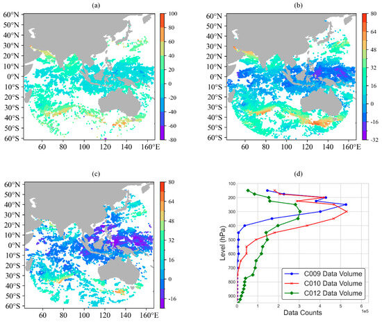
Figure 1.
The horizontal distribution of the upper-level water vapor channel (a), C009), mid-level water vapor channel (b), C010), and infrared channel (c), C012) data at 00 UTC on 1 January 2020, and the vertical distribution of AMV data volume from 1 to 31 January for the three channels (d).
The distribution of FY-4A AMVs data is mainly observed in East Asia, the Western Pacific, and the Atlantic regions, as depicted in the figure. The data are primarily concentrated in the troposphere, specifically in mid-troposphere cloud systems, with the infrared channel (C012) providing the most information. The water vapor channel (C009 and C010) data are mainly concentrated in the upper and middle tropospheres and are denser than the infrared channel information. There is a higher number of observations for the water vapor channel data compared to the infrared channel. The peak of these observations occurs between 500 hPa and 200 hPa.
2.2. Reanalysis Data
Obtaining meteorological data usually involves direct observation and remote-sensing observation. Over the past few decades, there has been a significant accumulation of meteorological data due to continuous technological advancements. However, direct observation from meteorological stations is often spatially sparse due to observation conditions. Sparsity can help to smooth out mesoscale meteorological data when performing interpolation. The accuracy of remote-sensing observation data can be impacted by various factors, including cloud cover, changes in satellite orbit, and the lifespan of the satellite. As a result, there may be temporal discontinuities in the data [40]. To address these shortcomings and fully utilize the physical properties of massive meteorological datasets, an effective approach is to assimilate data from different sources into the numerical prediction system, a process known as reanalysis. Reanalysis produces long-term, comprehensive meteorological data that cover multiple elements and time periods. It is regarded as a highly effective method for determining past atmospheric conditions [41].
The ERA5 dataset from the European Centre for Medium-Range Weather Forecasts (ECMWF) is a highly accurate representation of weather conditions. It provides hourly data for over 240 atmospheric, land, and oceanic variables from 1950 to the present with a spatial resolution of 0.25° × 0.25° [42]. Multiple studies have demonstrated that ERA5 outperforms other reanalysis datasets in terms of data quality, spatial resolution, and temporal coverage [43,44], making it highly suitable for various data-driven analyses, especially those employing machine learning.
This study uses hourly multi-layer atmospheric data from ERA5 spanning a 36-month period, starting in January 2020 and ending in December 2022. The meteorological variables include upper-level wind fields, pressure fields, and temperature fields, with a spatial resolution of 0.25° × 0.25°. This dataset covers the entire globe and is vertically divided into 25 layers, fully encompassing the FY-4A AMVs data. Here is a visualization of the wind field at 00 UTC on 1 January 2020, as depicted in Figure 2.
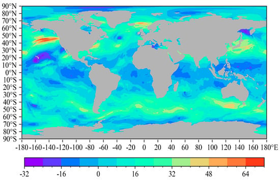
Figure 2.
Reanalysis data schematic (ERA5, 500 hPa U-Wind (m/s) stratified by atmospheric pressure; the color gradient represents wind speed).
2.3. Error Estimation
This research study utilizes two approaches to assess the validity of the research findings:
- (1)
- Using various quality-evaluation functions, such as Mean Absolute Error (MAE), Root Mean Square Error (RMSE), and correlation coefficient (R), along with a coefficient for measuring the consistency of wind field fluid characteristics.
- (2)
- Based on numerical weather prediction models and their corresponding assimilation systems, we can conduct assimilation forecast experiments to evaluate the real-world effectiveness of our research findings.
ERA5 data are widely accepted as the most accurate representation of the atmospheric state in this study. Here are the formulas for the four evaluation functions:
In the first three formulas, represents the FY-4A AMVs data, represents the ERA5 reanalysis data, and N is the sample size. The three statistical evaluation functions, as conventional quality-evaluation methods, can most directly test the error magnitude between the data and the relative true values. When the evaluation target is not correlated with the relative true values, the RMSE between the two can be considered the error value [45,46]. The MAE measures the discrepancy between the evaluation values and the relative true values, providing additional information to the RMSE about the evaluation error. The correlation coefficient R indicates the degree of dispersion of the evaluation data by measuring the correlation between the evaluation values and the relative true values.
For Formula (4), represents the consistency coefficient between the cloud motion vector at point i and the environmental wind vector at the nearby m points [14]. and are the consistency coefficients for wind direction and wind speed, respectively, with the specific calculation formulas as follows:
In the above formulas, represents the directional difference between wind vectors. According to the principle of continuity of fluid motion, there is a correlation and consistency in the speed and direction of fluid motion at neighboring points. If the corrected AMV data do not align with the environmental wind field at the corresponding levels, the consistency coefficient will decrease. Thus, the model’s ability to extract physical features can be assessed using this coefficient.
3. Methods
3.1. Dataset
Researchers frequently utilize deep learning in forecasting experiments involving meteorological data, often employing straightforward data-processing techniques. For instance, they may directly calibrate the data [47] or treat meteorological data as image data [21,48]. These methods streamline training processes, but there is a possibility of overlooking data correlations, which could result in the omission of certain features. As typical atmospheric wind field data, AMVs have distinct physical characteristics and cannot be simply treated as image data. Therefore, before constructing the model, it is necessary to reconstruct a dataset that fully reflects the feature correlations in AMV data based on its wind field characteristics.
The movement of air, in the context of AMVs, is mainly influenced by the pressure gradient force. There is a strong connection between the pressure field and the wind field. Pressure changes are fundamentally caused by uneven heating, which results in pressure variations at the same horizontal level, creating the pressure gradient force that drives wind. Thus, there is a connection between the temperature field and the wind field. Wind field data include two dimensions: wind speed and wind direction. In previous studies, researchers have often converted wind fields into U and V wind components and processed them separately [49]. This method ignores the dependency between U and V components, compromising the integrity of the original wind field information.
Creating a separate dataset for the wind field using the mentioned conditions could potentially lead to the omission of important physical attributes, resulting in less-than-optimal correction outcomes. Hence, this study integrates the wind field, pressure field, and temperature field into a multi-channel dataset without vector splitting the wind field. Instead, it utilizes comprehensive wind field data and incorporates pressure and temperature features to refine the wind field’s physical conditions. This process also involves making adjustments to the wind field and reassigning heights accordingly.
Firstly, horizontal processing is undertaken to consolidate data from various sources into a unified spatial and temporal resolution, facilitating subsequent comparisons and analyses. Since AMV data typically encompass only a subset of grid points within the satellite-detected cloud regions, with the remaining positions being absent, and considering that the ERA5 reanalysis data consist of global grid point data, which spatially exceed the area of the AMV data, it was determined, after multiple trials, to interpolate the reanalysis data onto the AMV grid points for the sake of research. Bilinear interpolation is employed in the horizontal direction, as illustrated in the accompanying Figure 3.
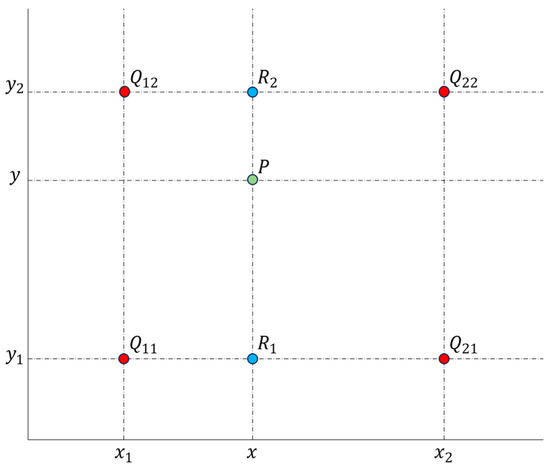
Figure 3.
Bilinear interpolation diagram. (The red dots represent the location of ERA5 data, the green dots represent the location of AMV data, and the blue dots represent the intermediate values.)
Point P represents a designated location for AMV data, while points to signify representative locations for ERA5 reanalysis data. Initially, the values of the two R points are computed using Equation (1), followed by the calculation of the data for point P through Equation (2).
Although each step of this method is linear in terms of sampled values and positions, the overall interpolation is not linear. For each AMV data point, interpolation is performed using the nearest four uniformly spaced ERA5 grid points, thereby deriving the horizontal data from the ERA5 dataset at the discrete AMV stations. In the vertical direction, analysis of multiple experimental results indicates negligible differences among various vertical interpolation methods, such as nearest neighbor interpolation, linear interpolation, and inverse distance weighting. Ultimately, linear interpolation is selected for processing vertical data. This results in a dataset of ERA5 reanalysis data labels that mirrors the structure of the AMV data. In terms of temporal alignment, the AMV data from FY-4A are generated every 3 h, producing data at 15 min intervals. The wind field data from ERA5 coincide perfectly with the AMV observation times, thereby eliminating the need for any further temporal interpolation.
3.2. Model Building
Meteorological data consist of spatiotemporal sequences that exhibit regular temporal patterns, including fluidity, continuity, and periodicity. Additionally, there are noticeable spatial correlations that coordinate and align meteorological elements across different points. For AMV data, wind field information is retrieved by observing the movement of clouds. As aggregations of water vapor, clouds are influenced in their formation, dissipation, movement, and evolution by the surrounding wind vectors. Under these circumstances, data from previous moments are related to the current data. At the same time, it is important for each observation point to be in sync with the surrounding wind field, ensuring the smooth flow of the wind. AMV data exhibit strong spatial correlations within a single dataset and strong temporal correlations across multiple datasets.
Thus, it is quite challenging to effectively correct errors in AMV data solely through time series prediction or spatial feature analysis. Therefore, it is essential to develop a model that can capture both the temporal and spatial characteristics of AMV data, enabling the integration of these features to obtain a comprehensive feature field.
3.2.1. Multi-Task Learning
Multi-task Learning (MTL) is a widely used technique in deep learning that enables the concurrent execution of multiple interconnected tasks, harnessing their processes to improve model performance. These tasks are usually interrelated, and MTL uses these correlations to enhance the generalization ability of single-task learning [50]. Researchers have extensively developed MTL, using it to forecast convective storms, lightning, and precipitation [51,52,53]. The main focus of MTL is “sharing”, leveraging the correlations between multiple tasks. MTL offers three different methods for sharing: instance sharing and parameter sharing. Feature sharing is a method that allows for the transfer of knowledge by identifying and utilizing common features across different tasks. Instance sharing is a valuable way to provide data instances for other tasks during recognition, allowing for the sharing of knowledge through identified instances. Model parameters can be shared across different tasks to enhance learning. This can be achieved through the use of regularization methods [54].
Considering the attributes of AMV data, MTL proves to be an optimal approach for extracting both temporal and spatial features, while also facilitating the sharing of various dimensional features. Therefore, this study adopts the feature-sharing method to construct the MTL skeleton model with two branch models: a temporal network and a spatial network. Figure 4 illustrates the basic MTL framework.
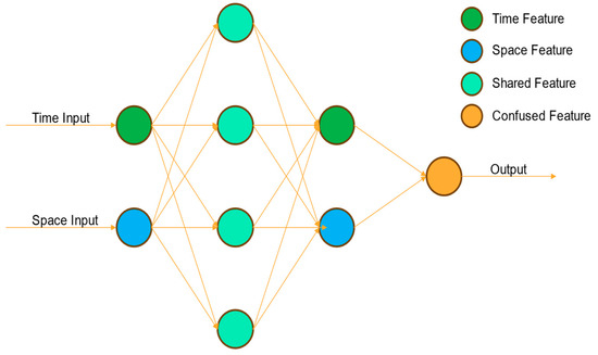
Figure 4.
Multi-task network schematic diagram (arrows represent data flow, circles represent different hidden layers).
3.2.2. Time Model
Time series analysis is commonly employed in meteorology due to the significant temporal correlation of meteorological data. Many scholars use classical models such as Recurrent Neural Network (RNN) or Long Short-Term Memory Network (LSTM) to conduct research [55,56,57]. In 2017, Ashish et al. [58] proposed the transformer model concept, demonstrating its powerful capability in modeling temporal data for Natural Language Processing (NLP). This model’s core technology incorporates an attention mechanism that enables it to comprehend sequences in a manner more akin to human understanding. In NLP, it can traverse correlations between any two words in a sequence, solving the problem of establishing long-term dependencies.
The transformer architecture effectively captures and utilizes the various time-scale features present in meteorological data with great precision. The attention mechanism can dynamically adjust the weights of data with large errors, reducing their impact on temporal features. Moreover, compared to LSTM, the transformer has higher computational efficiency, reducing costs. The transformer utilizes encoder–decoder architecture to handle input and output sequences. This architecture incorporates position encoding, multi-head attention mechanisms, and feed-forward networks. Position encoding enables the model to distinguish relative positions of input data, crucial for capturing temporal dynamics. The multi-head attention mechanism divides the query, key, and value vectors into multiple segments to enable separate computations, enabling the model to acquire more intricate feature representations. The feed-forward network in the transformer captures intricate connections between data sequences, facilitating accurate comprehension. Here is a visual representation of the transformer structure, as shown in Figure 5.
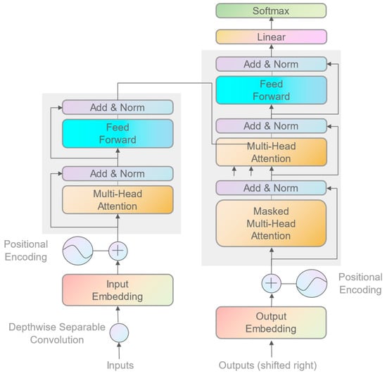
Figure 5.
Temporal branch network (based on the transformer network).
The present research utilizes the transformer architecture as the basis for the temporal branch model, making customized adjustments and enhancements to suit the specific characteristics of AMVs data. For data input, depthwise separable convolutions process each channel, using spatial filters to compress the data and adjust its features for transformer processing. By minimizing the number of parameters and computational complexity, the overall efficiency is improved. Wind field variations in data processing are caused by atmospheric motion and display temporal characteristics at multiple scales. The time characteristics of the wind field cannot only consider the influence of the near moment, but the long-term wind field evolution characteristics reflect more macroscopic characteristics, which can be regarded as a constraint condition of the current wind field. Thus, this study presents a module that utilizes a sliding time window to analyze the temporal characteristics of AMV data at different scales and generate corresponding features. The attention mechanism dynamically adjusts the influence weights of different time scales. Figure 6 demonstrates the analysis of time at multiple scales.
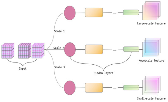
Figure 6.
The schematic diagram of the multi-scale feature analysis temporal branch network (hidden layers represent the transformer network, as shown in Figure 4).
3.2.3. Space Model
When it comes to spatial feature extraction, numerous studies have demonstrated the remarkable ability of Convolutional Neural Networks (CNNs) to uncover intricate details in data. These networks have played a crucial role in advancing image recognition and classification tasks. CNNs have been widely applied in meteorology, particularly in meteorological remote sensing [59,60,61]. This study uses CNNs as the foundation for the spatial branch model, constructing encoder–decoder architecture to extract deep spatial features from AMV data. The specific structure is shown in Figure 7.
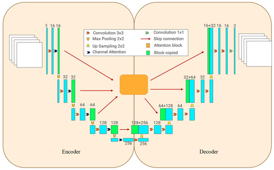
Figure 7.
Spatial branch network (based on Convolutional Neural Networks, the white squares represent the input and output datasets, and the blue squares represent the data undergoing convolution operations).
In the spatial branch model, the encoder module incrementally encodes the data, enhancing the model’s ability to perceive low-frequency features by gradually expanding its receptive field. During this phase, a channel attention module is created at each step to enable feature sharing between channels, constraining the wind field using the spatial features of the pressure and temperature fields. The decoder module systematically decodes the data and combines data of the same level through skip connections to merge information. This architecture facilitates better information and gradient flow, making the network easier to train and enhancing performance. It is capable of extracting detailed information at higher levels of the network and low-frequency information at lower levels. By incorporating skip connections, the integration of data ensures the preservation of all its features in a more comprehensive manner.
There is a variation in the importance of level features. In certain cases, feature extraction may not be enough, or there is a risk of losing significant information. Therefore, adjusting the weights of different levels is necessary. An attention module is created during the skip-connection process to dynamically adjust the weight of each level, ensuring complete extraction of AMV spatial features.
3.2.4. Time-Space Correction Network
This research employs various modules to construct a spatiotemporal network model for error correction of AMVs. The model is developed within a multi-task learning framework. The transformer serves as the foundation for the temporal branch model, while convolutional neural networks serve as the foundation for the spatial branch model. Enhancements are made to the model by considering the spatiotemporal characteristics of AMVs. The following is a visual representation of the model training process, as shown in Figure 8.
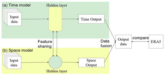
Figure 8.
Model-training process (yellow rectangles and green circles respectively represent hidden layers in the two branch models).
In the temporal branch model, the input consists of time series data, specifically AMV data collected over a certain period. After conducting numerous experiments and carefully evaluating both the quality of the model and the computational resources required, we have decided to choose a data-sequence length of 1 week. After format conversion using depthwise separable convolutions, the data undergo positional encoding before entering the encoder–decoder module to obtain temporal features at different time scales.
In the spatial branch model, the input is data at specific time points, focusing on the spatial structural characteristics of AMV data, including the relationships between observation points and the coupling between different channels. This branch acquires spatial features using the encoder–decoder module and then transfers them to the temporal features. At last, the attention mechanism combines temporal features of varying scales with spatial features.
3.3. Assimilation Experiment Settings
Assessing the accuracy of corrected AMV data through an assimilation system is crucial, and extensive research has been conducted on AMV data assimilation in the past. This study uses version 4.4 of the Weather Research and Forecasting (WRF) model and the WRF Data-Assimilation (WRFDA) system. The configuration consists of three nested layers, with resolutions of 27 km, 9 km, and 3 km. It is vertically divided into 41 layers, with the uppermost layer having a pressure of 50 hPa. This research utilizes the 3DVar assimilation method for conducting assimilation-forecast experiments. The assimilation region covers Southeast Asia and the Western Pacific, ranging from 40°S to 40°N and 100°E to 160°E. Figure 9 provides a schematic diagram of the region.
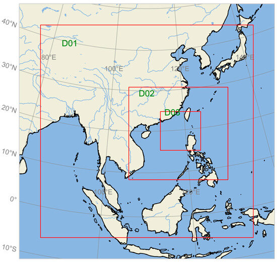
Figure 9.
Schematic diagram of the assimilation region. (The red blocks represent the nested areas of the model).
The model utilizes a cold start approach, incorporating FNL (Final Operational Global Analysis) data as the background field. The remaining model parameters are set according to the study conducted by Chen Yaodeng et al. [62]. In addition to the pre- and post-correction FY-4A AMVs data, conventional observational data from the Global Telecommunication System (GTS) are also assimilated. These include surface station observations (SYNOP), upper air observations (SOUND), ship observations (SHIP), aircraft reports (AIREP), buoy observations (BUOY), and so on.
4. Results
4.1. Error-Correction Effectiveness
Utilizing the quality-evaluation functions mentioned earlier, the study begins by using data from August 2022 as an illustrative example. Comparing the original data and corrected data at eight time points each day, we treat ERA5 reanalysis data as the relative true values. Figure 10 shows the model’s daily correction performance for that month.
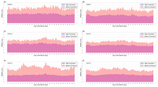
Figure 10.
RMSE comparison between data before correction and data after correction against ERA5 data in Month 8 (purple, data after correction; pink, data before correction). C009 represents the high-level water vapor channel, C010 denotes the low-level water vapor channel, and water vapor channel data mainly focus on the mid-to-upper troposphere. C012 represents the infrared channel, with data primarily concentrated in the mid-level troposphere.
The errors in the AMV data from all three channels were significantly reduced due to model correction. To further verify the sustainability of the correction effect and to avoid the “false optimization” effect caused by data leakage, this study conducted an in-depth analysis of the correction effect using the data from November 2022. In November, Figure 11 displays the wind field errors before and after correction, while Figure 12 and Figure 13 illustrate the comparison of wind speed distributions before and after correction.
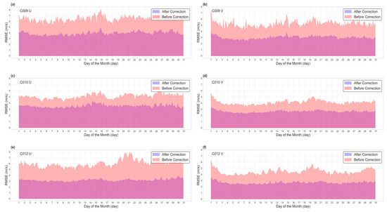
Figure 11.
RMSE comparison between data before correction and data after correction against ERA5 data in Month 11 (purple, data after correction; pink, data before correction). C009 characterizes the high-level water vapor channel, C010 represents the low-level water vapor channel, and water vapor channel data mainly focus on the mid-to-upper troposphere. C012 denotes the infrared channel, with data primarily concentrated in the mid-level troposphere.
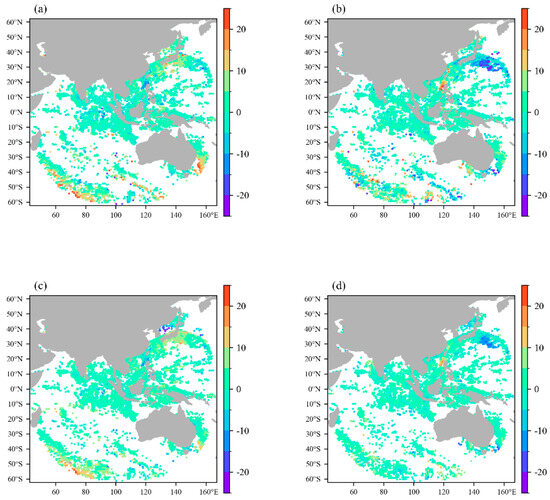
Figure 12.
Error distribution of the upper-level water vapor channel AMVs U and V wind vectors compared to ERA5 data before and after correction on 1 November, 2022, (a,b) represents the error distribution of U and V wind vectors before correction, (c,d) represents the error distribution after correction).
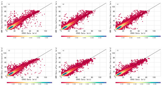
Figure 13.
Wind speed distribution of the three-channel AMV data compared to ERA5 data before and after correction on 1 November, 2022, (a–c) represents before correction, (d–f) represents after correction, with color representing data density; the darker the color, the more data.
It is worth noting that the error-correction effect continues to be significant even after a period of 3 months. Based on the daily comparison of the root mean square error (RMSE) in Figure 10, it is evident that the errors in all three channels have shown significant improvement. Furthermore, the errors have exhibited reduced fluctuations after the correction, suggesting a relatively stable correction effect. Among them, the correction effect of the C012 infrared channel is the most noticeable, with the smallest error fluctuation, while the effect on the C010 mid-level water vapor channel is slightly less pronounced.
According to the wind speed error chart (Figure 12), it is evident that the corrected wind speeds are significantly closer to the ERA5 reanalysis wind field. This further validates the model’s ability to correct AMV errors and highlights its effectiveness in smoothing out data errors. In Figure 13, the pre-correction data scatter around the diagonal but with significant deviations, and the areas of high data density are concentrated near the diagonal but with many points deviating from it, especially in regions with higher wind speeds (greater than 20 m/s). After making the necessary adjustments, the data now exhibit a more concentrated distribution along the diagonal, indicating improved consistency. Additionally, there has been a noticeable decrease in the number of data points that deviate from the diagonal. Overall, the consistency between the corrected AMVs data and the ERA5 data is significantly improved, and the dispersion is notably reduced.
In the study by Chen Yaodeng et al. [39], it was discovered that the data from FY-4A AMVs showed notable vertical error characteristics. To further examine the correction effects at different heights, the data from the three observation channels were stratified vertically and subjected to separate statistical analysis. This was done based on the stratification settings of the ERA5 reanalysis data as shown in Figure 14.
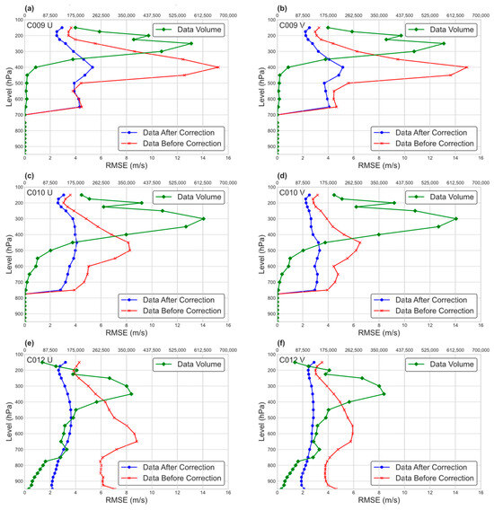
Figure 14.
RMSE comparison between data before correction and data after correction at different atmospheric pressure levels against ERA5 data (red, data before correction; blue, data after correction; green, data volume at respective pressure levels).
The statistical results show that the correction effects for AMV data at different pressure heights indicate that the correction effects are highly significant. From the data shown in the figure, it can be observed that for the two water vapor channels (C009 and C010), the error correction effects are quite evident at the levels with more data and more complete wind field information. Even at higher altitude levels with larger initial errors (500–300 hPa), the model’s ability to correct is highly noticeable. This is particularly true for the C009 channel, where the original AMV data had significant errors during this period, but after model correction, the optimization effect was very pronounced.
The data from the infrared channel (C012) were extensively optimized at various pressure height levels. The correction process resulted in consistently low root mean square error (RMSE), even at levels with a substantial amount of data. Additionally, influenced by the model dataset, the correction effects for U and V wind components were similar, without a significant difference between the two wind vector corrections. In addition, the vertical variation characteristics of AMV errors showed a significant reduction, suggesting the simultaneous optimization correction scheme is both feasible and effective.
4.2. Further Evaluation
Globally, the Quality Indicator (QI) code serves as a metric for assessing the data quality of AMVs. It assigns values on a scale of 1 to 100. Higher values indicate better quality of the original AMV data [62,63]. To further investigate the optimization effects of the model and avoid negative corrections on originally high-quality data, it is necessary to analyze the model’s correction and optimization effects on AMV data of different quality levels.
Figure 15 illustrates the impact of corrections on data with varying QI values. Based on the data presented in the figure, it can be observed that the model has a significant impact on correcting AMV data across various QI values. Particularly for data with QI > 85, where the original data errors are larger, the correction effects are more noticeable. Even for data with QI greater than 85, there is still a certain correction effect. When dealing with AMV data that have QI values close to 100, which can be considered as being “correct”, the impact of correction is minimal. This further demonstrates that the model does not simply approximate the data to the ERA5 data during error correction. Instead, it depends on the relationships between various element fields to limit the wind field, ensuring accurate adjustments without the risk of overfitting.

Figure 15.
RMSE comparison between data before correction and data after correction at different QI against ERA5 data (red, data before correction; blue, data after correction; green, data volume at respective QI).
RMSE, MAE, and R all judge the errors of AMV data from a statistical standpoint. Nevertheless, the data from AMVs, being actual atmospheric wind field data, display distinct fluid physical characteristics. Therefore, it is necessary to use the fluid consistency coefficient to assess the quality of wind field characteristics. Figure 16 presents the evaluation results of the fluid consistency coefficient for the entire month of November. The model clearly demonstrates notable enhancements in specific statistical error metrics and also incorporates optimizations to ensure smooth continuity of the entire wind field.
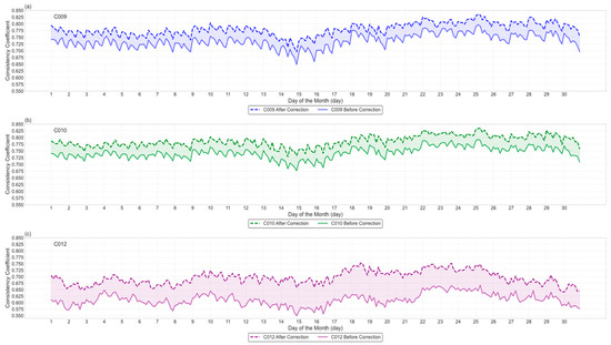
Figure 16.
Consistency coefficient comparison between data before correction and data after correction against ERA5 data (dotted line, data before correction; solid line, data after correction). C009 represents the high-level water vapor channel, C010 represents the low-level water vapor channel, and water vapor channel data mainly focus on the mid-to-upper troposphere. C012 represents the infrared channel, with data primarily concentrated in the mid-level troposphere.
Table 1 and Table 2 display the monthly average outcomes of the four evaluation functions throughout November 2022. These results are presented both before and after correction and are based on various observation channels of the AMV data.

Table 1.
Monthly average comparison results of the four evaluation functions (U wind vector, B–C represents pre-correction data, A–C represents post-correction data).

Table 2.
Monthly average comparison results of the four evaluation functions (V wind vector, B–C represents pre-correction data, A–C represents post-correction data).
Based on the evaluation results that consider mathematical statistics and physical characteristics, the model showcases exceptional performance. The quality of the corrected data has significantly improved, and the corrected wind field characteristics better conform to actual fluid characteristics. Conventional methods for preprocessing AMV data usually entail comparing it directly with reanalysis data and then eliminating data with significant deviations. As a result, some AMV data are often lost before entering the assimilation system. In contrast, the error correction method in this study optimizes errors while preserving the integrity of the data.
This study delves deeper into the cost of training the model. We performed model training using varying data volumes, specifically 6 months, 12 months, and 24 months of data. (The test data used in this study are all from November 2022, while the training set is based on data up to August 2022, going back to the corresponding months. For example, the training data for 6 months include data from February 2022 to August 2022, and the training data for 12 months include data from August 2021 to August 2022.) Following that, we conducted quality evaluations of the respective models. Figure 17 presents the respective quality-evaluation results. The results indicate that a data period of 6 months is enough to achieve favorable error correction outcomes for AMV data. Furthermore, as the data volume increases, the correction effect continues to improve.
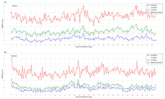
Figure 17.
Analysis of model correction results with training data of different periods (red represents the original root mean square error, green represents the root mean square error corrected by the model trained with 6 months of data, pink represents the root mean square error corrected by the model trained with 12 months of data, and blue represents the root mean square error corrected by the model trained with 24 months of data).
4.3. Assimilation Experiment Results
This study involved four assimilation experiments utilizing the WRF and WRFDA systems:
- (1)
- Assimilation of single-channel AMVs data before error correction (BC-Single);
- (2)
- Assimilation of single-channel AMVs data after error correction (AC-Single);
- (3)
- Assimilation of multi-channel AMVs data before error correction (BC-Multi);
- (4)
- Assimilation of multi-channel AMVs data after error correction (AC-Multi).
In order to assess the effect of error correction on assimilation experiments, the assimilated analysis fields were compared with ERA5 data to determine any differences in impact. Figure 18 presents the vertical profiles of root mean square error (RMSE) for four variables (u and v wind fields, temperature field t, and relative humidity rh). The figure demonstrates that the main improvements brought by the corrected AMVs data primarily exhibit improvements in the wind fields at higher altitudes. For the C009 and C010 water vapor channels, the improvements are primarily above the 500 hPa level, with the most significant improvements around 450–300 hPa, which is consistent with the vertical profile characteristics of their own observational errors. The data distribution of the C012 infrared channel covers a wider vertical range, impacting a broader range of meteorological elements. The figure indicates that the C012 infrared channel data quality significantly improves after model error correction compared to the two water vapor channels. In addition, despite the presence of minor initial errors, the corrected data demonstrate noticeable optimization effects on the upper-level temperature field.
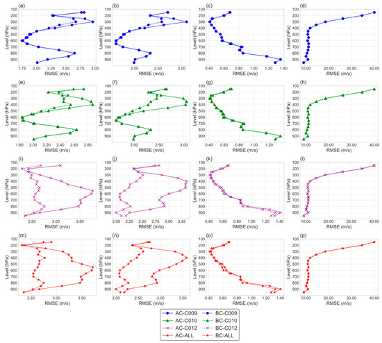
Figure 18.
Vertical profiles of root mean square error (RMSE) for the three-dimensional variational assimilation experiment results of AMVs data before and after correction for different channels (U wind vector: (a,e,i,m); V wind vector: (b,f,j,n); temperature: (c,g,k,o); relative humidity: (d,h,l,p); blue represents the C009 channel, green represents the C010 channel, purple represents the C012 channel, and red represents the multi-channel fusion; solid lines represent pre-correction data, dashed lines represent post-correction data).
Figure 19 and Table 3 display the cost and gradient functions throughout the assimilation process. They also show the observation innovations and analysis residuals of the AMV data before and after correction.
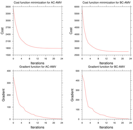
Figure 19.
Loss and gradient functions in the assimilation experiments before and after correction for C009 channel data (AC-AMVs represent the corrected AMV data, BC-AMVs represent the pre-correction AMV data).

Table 3.
Observation innovations (OI) and analysis residuals (AO) of the three-channel AMVs data before and after correction.
By examining the figures and tables, it becomes clear that the data from the three channels have distinct impacts on the wind field adjustments resulting from assimilation. Additionally, the adjustment heights exhibit significant variations. Therefore, based on the preliminary statistical results, this study proposes a new optimization strategy for the cross-fusion of data from different channels during multi-channel data-assimilation experiments:
- (1)
- When analyzing the data, it is important to consider the proximity of each data point in terms of both horizontal distance and pressure height. In this study, a close horizontal distance is defined as 0.5 degrees of latitude and longitude, while a similar pressure height is determined by data within 50 hPa of each other. By considering these factors, we can ensure that we are comparing data points that are in the same pressure layer and are geographically close to each other. If multiple data points exist simultaneously, make the following judgments: if the data point is located between 150–300 hPa, prioritize selecting data from the C009 channel; if the data point is between 300–500 hPa, prioritize selecting data from the C010 channel; if the data point is below 500 hPa, prioritize selecting data from the C012 channel. If there are multiple data points from the same channel, select the data with the higher QI value;
- (2)
- When there is a single data point within the same horizontal distance and height layer, it should be used;
- (3)
- When data points are spread out across various height layers but have the same horizontal distance, it is recommended to utilize all of them.
Taking the data from 1 November as an example, the optimized data showed better assimilation quality, particularly in adjusting the upper wind field. Additionally, some optimization was done to fine-tune the upper-temperature field. Here are the results of the assimilation experiment, as shown in Figure 20.
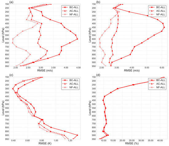
Figure 20.
Comparison of multi-channel fusion before and after improvement on 1 November, 2022: (a) is the U wind vector, (b) is the V wind vector, (c) is the temperature, (d) is the relative humidity; BC-ALL means before correction, AC-ALL means after correction, NF-ALL means new fusion method.
5. Discussions
Remote-sensing data from meteorological satellites play a crucial role in numerical weather prediction (NWP). However, there is still room for enhancing the accuracy of the data due to inherent errors in the observation and retrieval processes. As one of the meteorological remote-sensing data, atmospheric motion vectors (AMVs) play a crucial role in refining upper-level wind fields. However, the data characteristics of AMVs are complex, exhibiting strong temporal continuity and high spatial complexity. This research focuses on using AMVs as an example to enhance the initial field quality of NWP systems, optimize observation errors, and improve NWP performance. The goal is to improve the quality of meteorological satellite remote-sensing data. It breaks through the limitations of conventional preprocessing methods by using high-quality reanalysis data as relative true values and explores the effect of deep learning on correcting observation errors. A deep-learning network model was constructed to adapt to spatiotemporal characteristics of the data retrieved from FY-4A AMVs and ERA5 reanalysis. Here are the benefits of the model:
- (1)
- By analyzing the temporal and spatial aspects of AMVs independently and combining their features, the model effectively utilizes the unique data properties of AMVs and improves its ability to extract and fit features;
- (2)
- The multi-scale temporal dimension module set for AMV temporal characteristics effectively extracts temporal features, retaining long-term continuous features and capturing small-scale variation features, thus making the wind field’s temporal continuity more complete;
- (3)
- In the spatial dimension, a setup with multiple layers for encoding and decoding is utilized. This setup not only learns the larger spatial features of AMVs but also improves the ability to capture finer details. The channel attention module, created separately, aids in constraining the features of AMVs by considering the pressure and temperature field characteristics, thereby enhancing their physical attributes.
The analysis results using relevant quality-evaluation functions, fluid consistency tests, and NWP assimilation systems for error correction results indicate:
- (1)
- The model’s correction effect has a long-lasting duration. In challenging circumstances where there is a lack of new data for training, the model’s correction effect can remain stable for a minimum of 4 months;
- (2)
- Deep-learning technology can effectively correct AMV errors, showing significant correction effects across various dimensions, including daily observation errors of different channels, observation errors at different pressure levels, and observation errors with different QI quality labels;
- (3)
- As the amount of data increases, the error-correction capabilities of deep-learning technology can be further enhanced. By utilizing extensive historical observation data and top-notch reanalysis data, the model’s ability to correct errors will enhance as it continuously receives and undergoes training with more data;
- (4)
- The WRFDA assimilation experiment results further confirm the effectiveness of AMV error correction. The assimilation effect of corrected AMV data is significantly enhanced, and the newly set multi-channel fusion optimization strategy can further improve the assimilation effect of AMVs data.
The results of this research highlight the feasibility and effectiveness of utilizing deep-learning technology to correct errors in meteorological remote-sensing data. For further improvement in research results, the next step will be to conduct error-correction experiments on a wider range of meteorological remote-sensing data, including altimeter and scatterometer data. Additionally, incorporating more input data, such as longer time spans and additional channels, will be essential.
Author Contributions
All authors contributed significantly to this manuscript. Specific contributions include data collection, H.C. and H.L.; data analysis, H.C. and J.Z.; methodology, H.C., X.X., J.Y. and Y.Z.; manuscript preparation, H.C., H.L., B.L. and L.H. All authors have read and agreed to the published version of the manuscript.
Funding
This work was supported by the National Natural Science Foundation of China (Grant No. 41605070) and the National Key R&D Program of China [Grant Number 2022YFB3207304].
Data Availability Statement
No new data were created or analyzed in this study. The original contributions presented in the study are included in the article, further inquiries can be directed to the corresponding author.
Conflicts of Interest
The authors declare no conflicts of interest.
References
- Zeng, Q.C. Weather forecast—From empirical to physicomathematical theory and super-computing system engineering. Physics 2013, 42, 300–314. [Google Scholar]
- Benjamin, S.G.; Brown, J.M.; Brunet, G.; Lynch, P.; Saito, K.; Schlatter, T.W. 100 years of progress in forecasting and NWP applications. Meteorol. Monogr. 2019, 59, 13.1–13.67. [Google Scholar] [CrossRef]
- Bauer, P.; Thorpe, A.; Brunet, G. The quiet revolution of numerical weather prediction. Nature 2015, 525, 47–55. [Google Scholar] [CrossRef] [PubMed]
- Bannister, R.N. A review of operational methods of variational and ensemble-variational data assimilation. Q. J. R. Meteorol. Soc. 2017, 143, 607–633. [Google Scholar] [CrossRef]
- Zhang, L.; Liu, Y.; Liu, Y.; Gong, J.; Lu, H.; Jin, Z.; Tian, W.; Liu, G.; Zhou, B.; Zhao, B. The operational global four-dimensional variational data assimilation system at the China Meteorological Administration. Q. J. R. Meteorol. Soc. 2019, 145, 1882–1896. [Google Scholar] [CrossRef]
- Xue, J.S. Scientific issues and perspective of assimilation of meteorological satellite data. Acta Meteorol. Sin. 2009, 67, 903–911. [Google Scholar]
- Eyre, J.; English, S.; Forsythe, M. Assimilation of satellite data in numerical weather prediction. Part I: The early years. Q. J. R. Meteorol. Soc. 2020, 146, 49–68. [Google Scholar] [CrossRef]
- Sun, X.J.; Zhang, C.L.; Fang, L.; Lu, W.; Zhao, S.J.; Ye, S. A review of the technical system of spaceborne Doppler wind lidar and its assessment method. Natl. Remote Sens. Bull. 2022, 26, 1260–1273. [Google Scholar] [CrossRef]
- Velden, C.S.; Hayden, C.M.; Nieman SJ, W.; Paul Menzel, W.; Wanzong, S.; Goerss, J.S. Upper-tropospheric winds derived from geostationary satellite water vapor observations. Bull. Am. Meteorol. Soc. 1997, 78, 173. [Google Scholar] [CrossRef][Green Version]
- Jianmin, X.; Qisong, Z. Status review on atmospheric motion vectors-derivation and application. J. Appl. Meteorol. Sci. 2006, 17, 574–582. [Google Scholar]
- Lee, E.; Todling, R.; Karpowicz, B.M.; Jin, J.; Sewnath, A.; Park, S.K. Assessment of Geo-Kompsat-2A Atmospheric Motion Vector Data and Its Assimilation Impact in the GEOS Atmospheric Data Assimilation System. Remote Sens. 2022, 14, 5287. [Google Scholar] [CrossRef]
- Chen, K.; Guan, P. The Impacts of Assimilating Fengyun-4A Atmospheric Motion Vectors on Typhoon Forecasts. Atmosphere 2023, 14, 375. [Google Scholar] [CrossRef]
- Lyu, X.; Wang, X. The Impact of High-Density Airborne Observations and Atmospheric Motion Vector Observation Assimilation on the Prediction of Rapid Intensification of Hurricane Matthew (2016). Atmosphere 2024, 15, 395. [Google Scholar] [CrossRef]
- Yang, C.Y.; Lu, Q.F.; Jing, L. Numerical experiments of assimilation and forecasts by using dualchannels AMV products of FY-2 C based on height reassignment. J. PLA Univ. Sci. Technol. (Nat. Sci. Ed.)/Jiefangjun Ligong Daxue Xuebao 2012, 13, 6. [Google Scholar]
- Folger, K.; Weissmann, M. Lidar-Based Height Correction for the Assimilation of Atmospheric Motion Vectors. J. Appl. Meteorol. Climatol. 2016, 55, 2211–2227. [Google Scholar] [CrossRef]
- Hoffman, R.N.; Lukens, K.E.; Ide, K.; Garrett, K. A collocation study of atmospheric motion vectors (AMVs) compared to Aeolus wind profiles with a feature track correction (FTC) observation operator. Q. J. R. Meteorol. Soc. 2022, 148, 321–337. [Google Scholar] [CrossRef]
- Lean, K.; Bormann, N. Using Model Cloud Information to Reassign Low-Level Atmospheric Motion Vectors in the ECMWF Assimilation System. J. Appl. Meteorol. Climatol. 2023, 62, 361–376. [Google Scholar] [CrossRef]
- Jian, S.; Zhuo, C.; Heng, L.; Simeng, Q.; Xin, W.; Limin, Y.; Wei, X. Application of artificial intelligence technology to numerical weather prediction. J. Mech. Eng. 2021, 32, 1–11. [Google Scholar]
- Key, J.; Maslanik, J.A.; Schweiger, A.J. Classification of merged AVHRR and SMMR Arctic data with neural networks. Photogramm. Eng. Remote Sens. 1989, 55, 1331–1338. [Google Scholar]
- Dai, L.; Zhang, C.; Xue, L.; Ma, L.; Lu, X. Eyed tropical cyclone intensity objective estimation model based on infrared satellite image and relevance vector machine. J. Remote Sens. 2018, 22, 581–590. [Google Scholar] [CrossRef]
- Han, L.; Chen, M.; Chen, K.; Chen, H.; Zhang, Y.; Lu, B.; Song, L.; Qin, R. A Deep Learning Method for Bias Correction of ECMWF 24–240 h Forecasts. Adv. Atmos. Sci. 2021, 38, 1444–1459. [Google Scholar] [CrossRef]
- Ziyi, D.; Zhenhong, D.; Sensen, W.; Yadong, L.; Feng, Z.; Renyi, L. An automatic marine mesoscale eddy detection model based on improved U-Net network. Haiyang Xuebao 2022, 44, 123–131. [Google Scholar]
- Hess, P.; Boers, N. Deep Learning for Improving Numerical Weather Prediction of Heavy Rainfall. J. Adv. Model. Earth Syst. 2022, 14, e2021MS002765. [Google Scholar] [CrossRef]
- Litjens, G.; Kooi, T.; Bejnordi, B.E.; Setio, A.A.A.; Ciompi, F.; Ghafoorian, M.; van der Laak, J.A.W.M.; van Ginneken, B.; Sánchez, C.I. A survey on deep learning in medical image analysis. Med. Image Anal. 2017, 42, 60–88. [Google Scholar] [CrossRef]
- Liu, W.; Wang, Z.; Liu, X.; Zeng, N.; Liu, Y.; Alsaadi, F.E. A survey of deep neural network architectures and their applications. Neurocomputing 2017, 234, 11–26. [Google Scholar] [CrossRef]
- Pouyanfar, S.; Sadiq, S.; Yan, Y.; Tian, H.; Tao, Y.; Reyes, M.P.; Shyu, M.-L.; Chen, S.-C.; Iyengar, S.S. A Survey on Deep Learning: Algorithms, Techniques, and Applications. ACM Comput. Surv. 2018, 51, 92. [Google Scholar] [CrossRef]
- Alom, M.Z.; Taha, T.M.; Yakopcic, C.; Westberg, S.; Sidike, P.; Nasrin, M.S.; Hasan, M.; Van Essen, B.C.; Awwal, A.A.S.; Asari, V.K. A State-of-the-Art Survey on Deep Learning Theory and Architectures. Electronics 2019, 8, 292. [Google Scholar] [CrossRef]
- Li, T.; Wu, D.; Wang, L.; Yu, X. Recognition algorithm for deep convective clouds based on FY4A. Neural Comput. Appl. 2022, 34, 21067–21088. [Google Scholar] [CrossRef]
- Oh, S.G.; Son, S.W.; Kim, Y.H.; Park, C.; Ko, J.; Shin, K.; Ha, J.-H.; Lee, H. Deep learning model for heavy rainfall nowcasting in South Korea. Weather. Clim. Extrem. 2024, 44, 100652. [Google Scholar] [CrossRef]
- Wang, C.; Li, X. A Deep Learning Model for Estimating Tropical Cyclone Wind Radius from Geostationary Satellite Infrared Imagery. Mon. Weather. Rev. 2023, 151, 403–417. [Google Scholar] [CrossRef]
- Otsuka, M.; Seko, H.; Shimoji, K.; Yamashita, K. Characteristics of Himawari-8 Rapid Scan Atmospheric Motion Vectors Utilized in Mesoscale Data Assimilation. J. Meteorol. Soc. Jpn. 2018, 96, 111–131. [Google Scholar] [CrossRef]
- Velden, C.; Lewis, W.E.; Bresky, W.; Stettner, D.; Daniels, J.; Wanzong, S. Assimilation of high-resolution satellite-derived atmospheric motion vectors: Impact on HWRF forecasts of tropical cyclone track and intensity. Mon. Wea. Rev. 2017, 145, 1107–1125. [Google Scholar] [CrossRef]
- Kunii, M.; Otsuka, M.; Shimoji, K.; Seko, H. Ensemble data assimilation and forecast experiments for the September 2015 heavy rainfall event in Kanto and Tohoku Regions with atmospheric motion vectors from Himawari-8. SOLA 2016, 12, 209–214. [Google Scholar] [CrossRef][Green Version]
- Zhao, J.; Gao, J.; Jones, T.A.; Hu, J. Impact of Assimilating High-Resolution Atmospheric Motion Vectors on Convective Scale Short-Term Forecasts: 2. Assimilation Experiments of GOES-16 Satellite Derived Winds. J. Adv. Model. Earth Syst. 2021, 13, 1–25. [Google Scholar] [CrossRef]
- Lu, F.; Zhang, X.H.; Chen, B.Y.; Liu, H.; Wu, R.; Han, Q.; Zhang, Z.Q. FY-4 geostationary meteorological satellite imaging characteristics and its application prospects. J. Mar. Meteorol. 2017, 37, 1–12. [Google Scholar]
- Zhang, Z.Q.; Lu, F.; Fang, X.; Tang, S.; Zhang, X.; Xu, Y.; Han, W.; Nie, S.; Shen, Y.; Zhou, Y. Application and development of FY-4 meteorological satellite. Aerosp. Shanghai 2017, 34, 8–19. [Google Scholar]
- Wan, X.; Gong, J.; Han, W.; Tian, W. The Evaluation of FY-4A AMVs in GRAPES_RAFS. Meteorol. Mon. 2019, 45, 458–468. [Google Scholar]
- Chen, Y.; Shen, J.; Fan, S.; Meng, D.; Wang, C. Characteristics of Fengyun-4A Satellite Atmospheric Motion Vectors and Their Impacts on Data Assimilation. Adv. Atmos. Sci. 2020, 37, 1222–1238. [Google Scholar] [CrossRef]
- Chen, Y.; Shen, J.; Fan, S.; Wang, C. A study of the observational error statistics and assimilation applications of the FY-4A satellite atmospheric motion vector. Trans. Atmos Sci. 2021, 44, 418–427. [Google Scholar]
- Faghmous, J.H.; Kumar, V. A Big Data Guide to Understanding Climate Change: The Case for Theory-Guided Data Science. Big Data 2014, 2, 155–163. [Google Scholar] [CrossRef]
- Gheysari, A.F.; Maghoul, P.; Ojo, E.R.; Shalaby, A. Reliability of ERA5 and ERA5-Land reanalysis data in the Canadian Prairies. Theor. Appl. Climatol. 2024, 155, 3087–3098. [Google Scholar] [CrossRef]
- Hersbach, H.; Bell, B.; Berrisford, P.; Hirahara, S.; Horányi, A.; Muñoz-Sabater, J.; Nicolas, J.; Peubey, C.; Radu, R.; Schepers, D.; et al. The ERA5 global reanalysis. Q. J. R. Meteorol. Soc. 2020, 146, 1999–2049. [Google Scholar] [CrossRef]
- Graham, R.M.; Hudson, S.R.; Maturilli, M. Improved Performance of ERA5 in Arctic Gateway Relative to Four Global Atmospheric Reanalyses. Geophys. Res. Lett. 2019, 46, 6138–6147. [Google Scholar] [CrossRef]
- Taszarek, M.; Pilguj, N.; Allen, J.T.; Gensini, V.; Brooks, H.E.; Szuster, P. Comparison of Convective Parameters Derived from ERA5 and MERRA-2 with Rawinsonde Data over Europe and North America. J. Clim. 2021, 34, 3211–3237. [Google Scholar] [CrossRef]
- Benjamin, S.G.; Schwartz, B.E.; Cole, R.E. Accuracy of ACARS Wind and Temperature Observations Determined by Collocation. Weather. Forecast. 1999, 14, 1032. [Google Scholar] [CrossRef]
- Gao, F.; Zhang, X.Y.; Jacobs, N.A.; Huang, X.Y.; Zhang, X.; Childs, P.P. Estimation of TAMDAR Observational Error and Assimilation Experiments. Weather. Forecast. 2012, 27, 856–877. [Google Scholar] [CrossRef]
- Zhou, K.; Zheng, Y.; Li, B.; Dong, W.; Zhang, X. Forecasting Different Types of Convective Weather: A Deep Learning Approach. J. Meteorol. Res. 2019, 33, 797–809. [Google Scholar] [CrossRef]
- Zhang, W.; Han, L.; Sun, J.; Guo, H.; Dai, J. Application of Multi-channel 3D-cube Successive Convolution Network for Convective Storm Nowcasting. In Proceedings of the 2019 IEEE International Conference on Big Data (Big Data), Los Angeles, CA, USA, 9–12 December 2019. [Google Scholar]
- Liu, N.; Yan, Z.; Tong, X.; Jiang, J.; Li, H.; Xia, J.; Lou, X.; Ren, R.; Fang, Y. Meshless Surface Wind Speed Field Reconstruction Based on Machine Learning. Adv. Atmos. Sci. 2022, 39, 1721–1733. [Google Scholar] [CrossRef]
- Zhang, Y.; Yang, Q. A survey on multi-task learning. IEEE Trans. Knowl. Data Eng. 2021, 34, 5586–5609. [Google Scholar] [CrossRef]
- Ruiz, C.; Alaíz, C.M.; Dorronsoro, J.R. A survey on kernel-based multi-task learning. Neurocomputing 2024, 577, 127255. [Google Scholar] [CrossRef]
- Li, Y.; Liu, Y.; Sun, R.; Guo, F.; Xu, X.; Xu, H. Convective Storm VIL and Lightning Nowcasting Using Satellite and Weather Radar Measurements Based on Multi-Task Learning Models. Adv. Atmos. Sci. 2023, 40, 887–899. [Google Scholar] [CrossRef]
- Chu, W.T.; Liang, Y.H.; Ho, K.C. Visual Weather Property Prediction by Multi-Task Learning and Two-Dimensional RNNs. Atmosphere 2021, 12, 584. [Google Scholar] [CrossRef]
- Qiu, M.; Zhao, P.; Zhang, K.; Huang, J.; Shi, X.; Wang, X.; Chu, W. A short-term rainfall prediction model using multi-task convolutional neural networks. In Proceedings of the 2017 IEEE International Conference on Data Mining (ICDM), New Orleans, LA, USA, 18–21 November 2017; IEEE: New York City, NY, USA, 2017; pp. 395–404. [Google Scholar]
- Ni, L.; Wang, D.; Singh, V.P.; Wu, J.; Wang, Y.; Tao, Y.; Zhang, J. Streamflow and rainfall forecasting by two long short-term memory-based models. J. Hydrol. 2020, 583, 124296. [Google Scholar] [CrossRef]
- Wang, F.; Cao, Y.; Wang, Q.; Zhang, T.; Su, D. Estimating Precipitation Using LSTM-Based Raindrop Spectrum in Guizhou. Atmosphere 2023, 14, 1031. [Google Scholar] [CrossRef]
- Parasyris, A.; Alexandrakis, G.; Kozyrakis, G.V.; Spanoudaki, K.; Kampanis, N.A. Predicting Meteorological Variables on Local Level with SARIMA, LSTM and Hybrid Techniques. Atmosphere 2022, 13, 878. [Google Scholar] [CrossRef]
- Vaswani, A.; Shazeer, N.; Parmar, N.; Uszkoreit, J.; Jones, L.; Gomez, A.N.; Kaiser, L.; Polosukhin, I. Attention Is All You Need. Learning 2017, 5. [Google Scholar]
- Huang, J.; Zhang, Y.; Ma, G.; Zhu, L.; Tian, W. Research on Precipitation Estimation Algorithm from Fengyun-4 Satellite Based on Improved U-Net. J. Comput. Eng. Appl. 2023, 59, 285. [Google Scholar]
- Mishra, S.; Guhathakurta, P.K. Identification of Cloud Types for Meteorological Satellite Images: A Character-Based CNN-LSTM Hybrid Caption Model. In Proceedings of the International Conference on Computational Intelligence in Communications and Business Analytics, Kalyani, India, 27–28 January 2023; Springer Nature: Cham, Switzerland, 2023; pp. 199–212. [Google Scholar]
- Kattenborn, T.; Leitloff, J.; Schiefer, F.; Hinz, S. Review on Convolutional Neural Networks (CNN) in vegetation remote sensing. ISPRS J. Photogramm. Remote Sens. 2021, 173, 24–49. [Google Scholar] [CrossRef]
- Velden, C.S.; Olander, T.L.; Wanzong, S. The Impact of Multispectral GOES-8 Wind Information on Atlantic Tropical Cyclone Track Forecasts in 1995. Part I: Dataset Methodology, Description, and Case Analysis. Mon. Weather. Rev. 1998, 126, 1202–1218. [Google Scholar] [CrossRef]
- Xue, C.B.; Gong, J.D.; He, C.F.; Wang, R.C. Quality control of cloud derived wind vectors from geostationary meteorological satellites with its application to data assimilation system. J. Appl. Meteor. Sci. 2013, 24, 356–364. [Google Scholar]
Disclaimer/Publisher’s Note: The statements, opinions and data contained in all publications are solely those of the individual author(s) and contributor(s) and not of MDPI and/or the editor(s). MDPI and/or the editor(s) disclaim responsibility for any injury to people or property resulting from any ideas, methods, instructions or products referred to in the content. |
© 2024 by the authors. Licensee MDPI, Basel, Switzerland. This article is an open access article distributed under the terms and conditions of the Creative Commons Attribution (CC BY) license (https://creativecommons.org/licenses/by/4.0/).