Article

A Multi-Task Convolutional Neural Network Relative Radiometric Calibration Based on Temporal Information

1
The Department of Computer Science, Harbin Institute of Technology, Shenzhen 518055, China
2
National Satellite Meteorological Center, Beijing 100086, China
3
National Meteorological Center, Beijing 100086, China
*
Author to whom correspondence should be addressed.
Remote Sens. 2024, 16(17), 3346; https://doi.org/10.3390/rs16173346
Submission received: 9 July 2024 / Revised: 30 August 2024 / Accepted: 4 September 2024 / Published: 9 September 2024

Abstract

:
Due to the continuous degradation of onboard satellite instruments over time, satellite images undergo degradation, necessitating calibration for tasks reliant on satellite data. The previous relative radiometric calibration methods are mainly categorized into traditional methods and deep learning methods. The traditional methods involve complex computations for each calibration, while deep-learning-based approaches tend to oversimplify the calibration process, utilizing generic computer vision models without tailored structures for calibration tasks. In this paper, we address the unique challenges of calibration by introducing a novel approach: a multi-task convolutional neural network calibration model leveraging temporal information. This pioneering method is the first to integrate temporal dynamics into the architecture of neural network calibration models. Extensive experiments conducted on the FY3A/B/C VIRR datasets showcase the superior performance of our approach compared to the existing state-of-the-art traditional and deep learning methods. Furthermore, tests with various backbones confirm the broad applicability of our framework across different convolutional neural networks.

Graphical Abstract

1. Introduction

Satellite remote sensing image data are increasingly used in a wide range of fields such as meteorological forecasting, weather analysis, environmental disaster response and monitoring of agricultural land resources. However, the performance of satellite sensors is compromised by operational environments and the aging of devices during in-orbit operations, while natural factors such as lighting conditions, atmospheric composition and meteorological conditions also greatly affect the spectral data of features acquired by the sensors. These factors together lead to the problem of distortion in the acquired satellite data, which has a significant impact on further applications. Therefore, the calibration process of satellite sensors has become a crucial step in satellite big data mining, which is defined as the establishment of a quantitative conversion relationship between the output value of the thermal remote sensor and the brightness value of the incident radiation. In order to ensure that the acquired data can truly reflect the changes in the ground features and to improve the quality and reliability of the data, the calibration has become an indispensable part of the satellite data application.
The traditional calibration methods are mainly divided into two categories: absolute radiometric calibration and relative radiometric calibration. Absolute radiometric calibration usually has to dispatch technicians to conduct field surveys for obtaining the surface reflectance during the satellite transit [1]. Alternative methods involve using ground-based automatic station data. For example, Chen Y. et al. used ground-based automatic station data to realize the calibration of the MERSI-II sensors through the BRDF calibration [2], and D. Rudolf et al. used Absolute radiometric calibration for the novel DLR “Kalibri” transponder [3]. However, these methods are often time-consuming, labor-intensive and costly, and obtaining accurate reference data for historical datasets is challenging. Therefore, the relative radiometric calibration method is more commonly used nowadays. Relative radiometric calibration leverages the statistical characteristics of the pixel gray values within the image itself to establish a correction equation between the target image and a reference image, facilitating direct radiometric calibration [4], which is more time-saving and labor-saving than the absolute radiometric calibration and can even yield superior results.
The concept of relative radiometric calibration is based on the assumption that the radiance response is linearly related to digital counts. The calibration process adjusts the gain of this linear response to match the radiance that would be consistent with the initial radiance if the Earth’s reflectance were constant. It assumes that at different times at the same place on the two images, the existence of invariant characteristics of the surface reflectance of the approximate linear changes, so to find out the invariant characteristics of the point for linear regression, this linear regression is the value of the ratio of the relative sensitivity coefficients of the two images. Then, the target image, by multiplying this ratio coefficient, can be realized by correcting the reference image, the process is called calibration. Relative radiometric calibration encompasses various methods, with one of the simplest being the histogram matching (HM) method. HM uses a statistical method to calculate the cumulative histogram of the original image and the reference image, followed by a matching transformation to align their hue contrasts, thereby correcting the target image to the reference image [5]. Although this method is straightforward and user-friendly, its accuracy is often suboptimal. Schott and Salvaggio introduced the concept of pseudo-invariant features (PIFs) [6] in 1988, selecting stable reflectance spectra features with minimal change over time as sample points for radiometric correction. However, manually selecting invariant feature points can be subjective, as these points are not truly invariant. However, the concept of no-change pixels (NCPs) opened the door to linear regression for relative radiometric calibration, and after that, Nielsen, Conradsen et al. proposed a novel method of multivariate alteration detection (MAD) [7] by integrating the radiometric information of each spectral band through a statistical analysis. This approach reduced the influence of subjective judgment by utilizing a mathematical method of statistical analysis for NCP identification. Moreover, the authors enhanced their methodology by introducing a weighting coefficient and a loop, leading to the development of the iteratively reweighted multivariate alteration detection (IR-MAD) method [8]. IR-MAD utilizes iterative reweighting, which updates the weight value of each pixel point. Large weights are assigned to observation points exhibiting minimal change over time. This is carried out until the correlation coefficient of the typical correlation analysis converges or is smaller than a certain threshold. The pixel point with the largest weight in the final result is selected as the stable pixel sample point detected in the image pair. Others are image regression (IR) [9], dark setbright (DB) set normalization [10] and no-change (NC) set radiometric normalization [11]. Overall, traditional calibration methods typically require the identification of NCPs, presenting a considerable challenge in the calibration process. The initial phase involves eliminating subjectivity and thoroughly filtering the data to ensure consistency among the identified points. However, this process is inherently uncertain, lacking a definitive method for determining the number of points or establishing a standard threshold for identification.
With the rapid development of deep learning in recent years, many people have started to use neural networks in remote sensing, such as Velloso et al. for radiometric normalization of land cover change detection [12] and G. Yang et al. for estimating sub-pixel temperature [13], as opposed to the research on intelligent self-calibration, because the advantage of intelligent self-calibration is that it can bypass the identification of pseudo-invariant feature points and has a faster speed and less computational effort. Convolutional neural networks [14], a powerful tool in the field of computer vision, have also achieved good results in the field of remote sensing, for example, mapping the continuous cover of invasive noxious weed species [15], sea surface temperature reconstruction [16] and GNSS deformation monitoring forecasting [17]. Meanwhile, they also have applications in calibration. In the relative radiometric calibration method using the convolutional neural network proposed by Xutao Li et al. [18], they directly try to use deep learning to solve the relative radiometric calibration of on-orbit satellites and solve the calibration task as an image classification problem in the field of computer vision. However, there are two primary weaknesses with this approach. Firstly, directly applying computer vision (CV) models for calibration is evidently insufficient. Calibration focuses on examining the relationship and differences between the reference image and the target image, which involves concatenating the two images along the channel dimension. In traditional CV tasks, channels typically represent RGB values, and the relationships between these channels are not closely related to calibration. Therefore, when designing deep-learning-based calibration methods, it is inadequate to directly transplant CV models. Instead, a new framework needs to be designed to assist the model in exploring the correlations between channels specifically for calibration purposes. Secondly, temporal information is critically important in calibration. Generally, the larger the time span between two images, the smaller the corresponding relative sensitivity coefficient. For deep learning, this temporal information is crucial for fitting the final labels. However, the previous work has not sufficiently investigated this aspect.
Therefore, we propose a relative radiometric calibration method using deep learning with a multi-task module. This method emphasizes the crucial temporal information in calibration by incorporating time as an auxiliary task within a multi-task module. Additionally, since the temporal information used is the time span between the reference and target images, the multi-task module can effectively focus on the correlations between the two images across different channels, aligning seamlessly with the specific calibration requirements. Finally, our experiments show that the framework surpasses state-of-the-art methods, validating the effectiveness of incorporating the time span as a task rather than merely a feature across various neural networks. Figure 1 presents the calibration results visualized using multisite (MST) [19] calibration, IR-MAD, VGG and our method. In summary, our contributions are as follows:
1.
We propose a time-based multi-task neural network framework for calibration, demonstrating broad applicability and compatibility with numerous CNN models, thereby enhancing the calibration results.
2.
We introduce time span information by using the interval between the reference image and the target image for calibration, effectively prompting the model to recognize the importance of temporal factors in determining the ratio coefficients.
3.
Leveraging the multi-task module and time information, our proposed approach achieves state-of-the-art performance on the VIRR sensor dataset from FY3A and FY3C satellites, with improvements of 9.38% for FY3A and 22.00% for FY3C compared to the current state-of-the-art methods.

2. Preliminary

The first step in the calibration process is to establish a conversion relationship between the raw satellite digital numbers (DNs) and the top of atmosphere (TOA) reflectance. This relationship is defined as follows:
ρ c = slope c · DN c + offset c ) d 2 cos ( θ )
where ρ c is the TOA reflectance corresponding to channel c, and DN c is the DN value of channel c. Both slope c and offset c are the absolute calibration coefficients of channel c prior to launch, d is the Sun–Earth distance, and θ is the solar zenith angle. With this formula, we can obtain the TOA reflectance for in-orbit calibration.
The calibration coefficients are divided into two categories: absolute calibration coefficients and relative calibration coefficients. The absolute calibration coefficients are the pre-launch calibration coefficients mentioned in the equation above. In contrast, relative calibration coefficients, which are the focus of this study, are used for in-orbit calibration to account for changes over time. Meanwhile, the sensitivity coefficient is the inverse of the correction coefficient. As mentioned above, the ultimate goal of calibration is to fit the ratio of the relative sensitivity coefficients of the two images. This is because there is such a relationship between the reference and target images and the relative sensitivity coefficients of both, shown as follows:
ρ c , t 1 N t 1 , t 2 S R c t 1 = ρ c , t 2 N t 1 , t 2 S R c t 2
S R c t 2 S R c t 1 = ρ c , t 2 N t 1 , t 2 ρ c , t 1 N t 1 , t 2 = m c t 1 , t 2
where N t 1 , t 2 represents the NCPs on the image at times t 1 and t 2 for channel c. The terms S R c t 1 and S R c t 2 denote the relative sensitivity coefficients corresponding to channel c at times t 1 and t 2 . By applying certain transformations to Equation (2), we derive Equation (3), where m c t 1 , t 2 is the parameter we need to fit. This parameter is highly correlated with the sensitivity coefficient of the input image.

3. Proposed Method

In this section, we show the comprehensive model of a multi-task convolutional neural network based on temporal information. Our method bypasses the detection of NCPs by directly fitting the ratio coefficients m c t 1 , t 2 , thereby avoiding the associated challenges and potential interferences. First, we introduce the overall architecture of the model, followed by detailed descriptions of the feature extraction module, the multi-task module and the composite loss computation within the multi-task module.

3.1. Overview of the Proposed Method

This section presents an overview of the network architecture, which comprises two primary modules: a feature extraction module and a multi-task module, shown in Figure 2.
The feature extraction module, containing convolutional and pooling layers, extracts features from images, addressing the low resolution and redundant information typical of remote sensing images. Given that crucial information may be localized at the pixel level, the module effectively filters out redundant and extraneous features, retaining only those essential for accurate label fitting.
The multi-task module further facilitates label fitting. It takes the output of the feature extraction module, stretches it into vectors and fits the respective labels. Recognizing that fitting a single branch may not fully exploit the available information, a multi-task module is employed to indirectly support the main task fitting through auxiliary task branches. In this module, the feature extraction module is shared across tasks during backpropagation, facilitating parameter updates in two ways: primarily tuning for the main task and secondarily for the auxiliary tasks. By combining the losses from both tasks into a composite loss, this approach ensures the effective utilization of image information for fitting m c t 1 , t 2 . Detailed explanations follow in the later subsections.

3.2. Feature Extraction Module

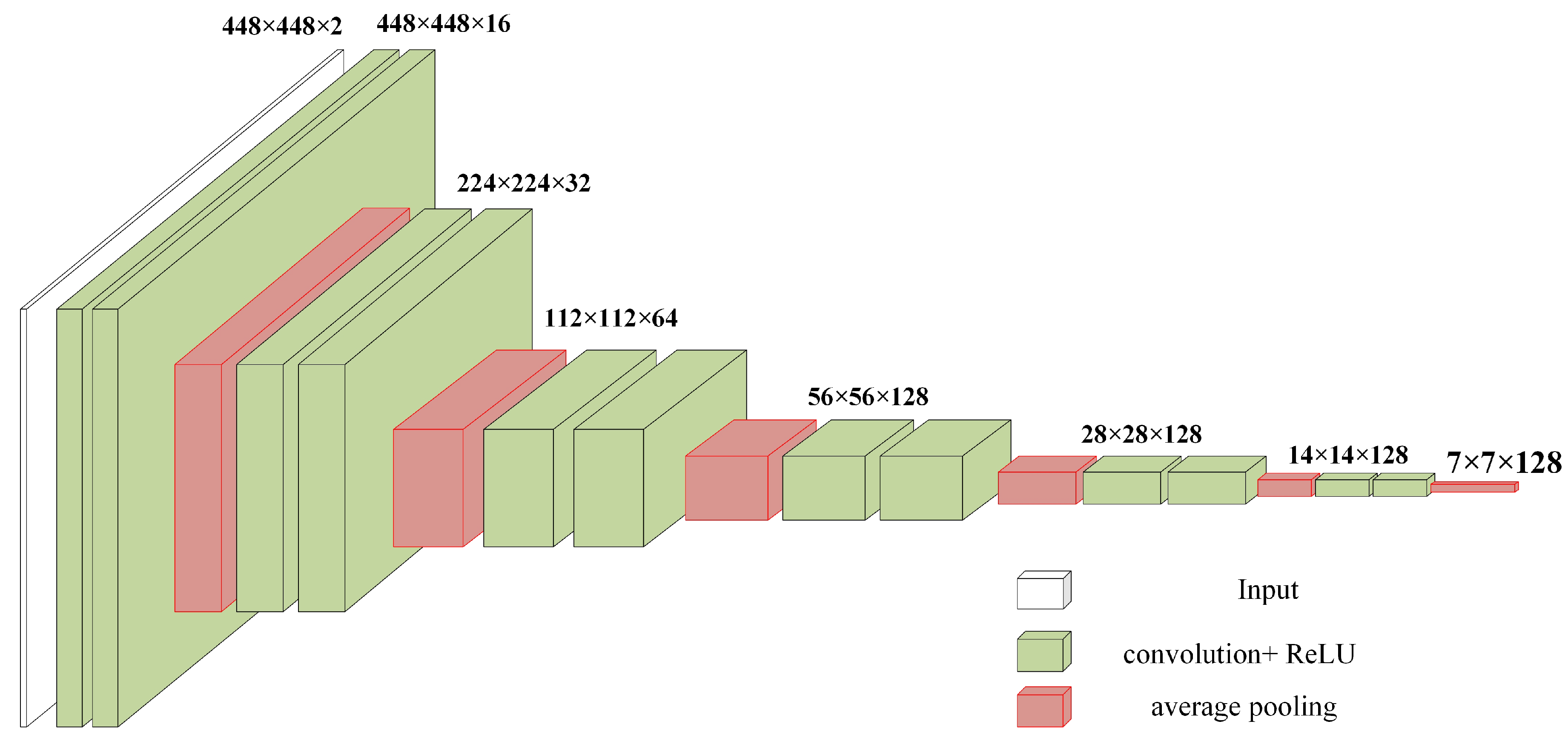
This paper introduces a feature extraction module inspired by a VGG-like network, as shown in Figure 3, with detailed parameters listed in Table 1. This module is an enhanced version of the VGG13 neural network [20] and consists of 12 layers. Each convolutional block, made up of two identical convolutional layers, aims to extract features from images of the same size. Following each convolutional block is a pooling layer, which downsamples the image to compress and filter features while expanding the channels to minimize information loss from downsampling.
Given that the input is a remote sensing image where each pixel represents a 1.1 km × 1.1 km area, small pixels can contain substantial information. Therefore, a 3 × 3 convolution size is used for small-area convolution. This captures detailed information, thus preventing important information from being lost due to convolution. Furthermore, the rectified linear unit (ReLU) is chosen as the activation function. The feature map sizes change as follows: 448→224→112→56→28→14→7.
In contrast to the VGG13 network, which uses max pooling to capture prominent features, this module focuses on background features rather than texture details. The research by Bolei Zhou et al. [21] demonstrated that average pooling has a localizable depth representation and is better at capturing deep details and background features. Therefore, average pooling is used for downsampling, positioned between two convolutional blocks as a downsampling transition layer. The channel variations are: 2→16→32→64→128→128→128.

3.3. Multi-Task Module

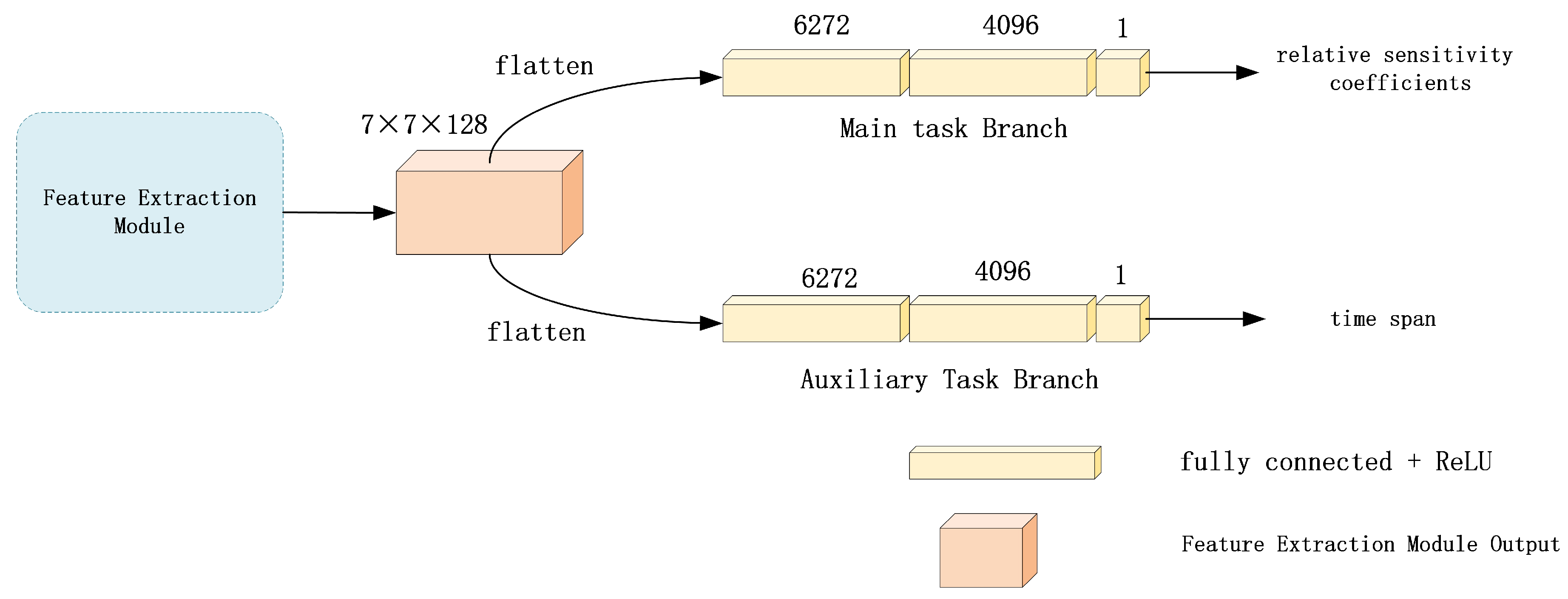
We propose a multi-task module based on time-assisted tasks to address the specific requirements of calibration. This module is illustrated in Figure 4. It is well-known that the cornerstone of calibration is obtaining the ratio coefficient m c t 1 , t 2 . The primary goal of calibration is to correct images that have undergone degradation due to factors such as atmospheric changes, instrument aging, and varying lighting conditions over time. Consequently, we posit that time information is uniquely critical for accurately fitting m c t 1 , t 2 .
Generally, as the time span increases, image degradation becomes progressively more severe. The calibration process involves multiplying the ratio coefficient m c t 1 , t 2 by the target image, thereby aligning the target image with the reference image. This implies that over longer time spans, the relative sensitivity coefficient decreases, exhibiting a non-linear relationship. Therefore, the greater the time difference between the target image and the reference image, the smaller the ratio coefficient m c t 1 , t 2 . This relationship is evident in the multisite MST calibration results [19], which also serve as the true values of the relative sensitivity coefficient used for training. This is shown in Figure 5.
The integration of temporal information is a key innovation of this paper. Typically, temporal information is incorporated as a feature input. However, we argue that this approach can result in the loss of information during the convolution and pooling processes. This issue is particularly pronounced in deep learning, where the depth of neural networks can cause temporal information to become overshadowed by redundant features, potentially leading to its ablation within the network and resulting in suboptimal performance in the final fitting.
To address this, we have adopted a multi-task module that uses time as a label value for auxiliary tasks. By treating time as a label, it effectively permeates the entire network and influences the network’s adjustments during backpropagation. Consequently, this approach allows temporal information to be effectively used throughout the network, even for deep neural networks with deep hierarchies, and ensures that it does not interfere with the fitting of the main task through the clever design of the composite loss. Moreover, we have conducted extensive experiments to validate the advantages of our method, which are detailed in the experimental section.
The multi-task module we design for temporal information fusion leverages the output of the feature extraction module. Initially presented as a matrix, this output undergoes flattening into a vector. Subsequently, the module branches into two multi-task pathways: a shared backbone and two specialized branches. Both branches are fitted using three fully connected layers. The primary task branch focuses on fitting m c t 1 , t 2 , while the auxiliary task branch fits the time span. This design ensures that temporal information is effectively integrated and leveraged throughout the entire network.

3.4. Composite Loss

In addition to task selection, multi-task training is crucial, and the configuration of the loss function is equally significant [22]. In this paper, we design a multi-task architecture with hard parameter sharing and make specific adjustments to the loss computation. First, we introduce a learnable parameter to regulate the weights of the main task (loss1) and the auxiliary task (loss2) during the loss generation. Given the hierarchical nature of these tasks, this coefficient is set between 0.1 and 0.4 to ensure that the main task contributes more significantly to the final calculated loss, thereby biasing the network towards the main task. The network is thus optimized with a preference for the primary task. The specific formula is presented as follows:
loss = loss 1 × ( 1 α ) + loss 2 × α
where loss 1 is the loss of main task, and loss 2 is the loss of auxiliary task. α is a learnable parameter that takes values from 0.1 to 0.4. Finally, loss is the composite loss.

4. Experiment

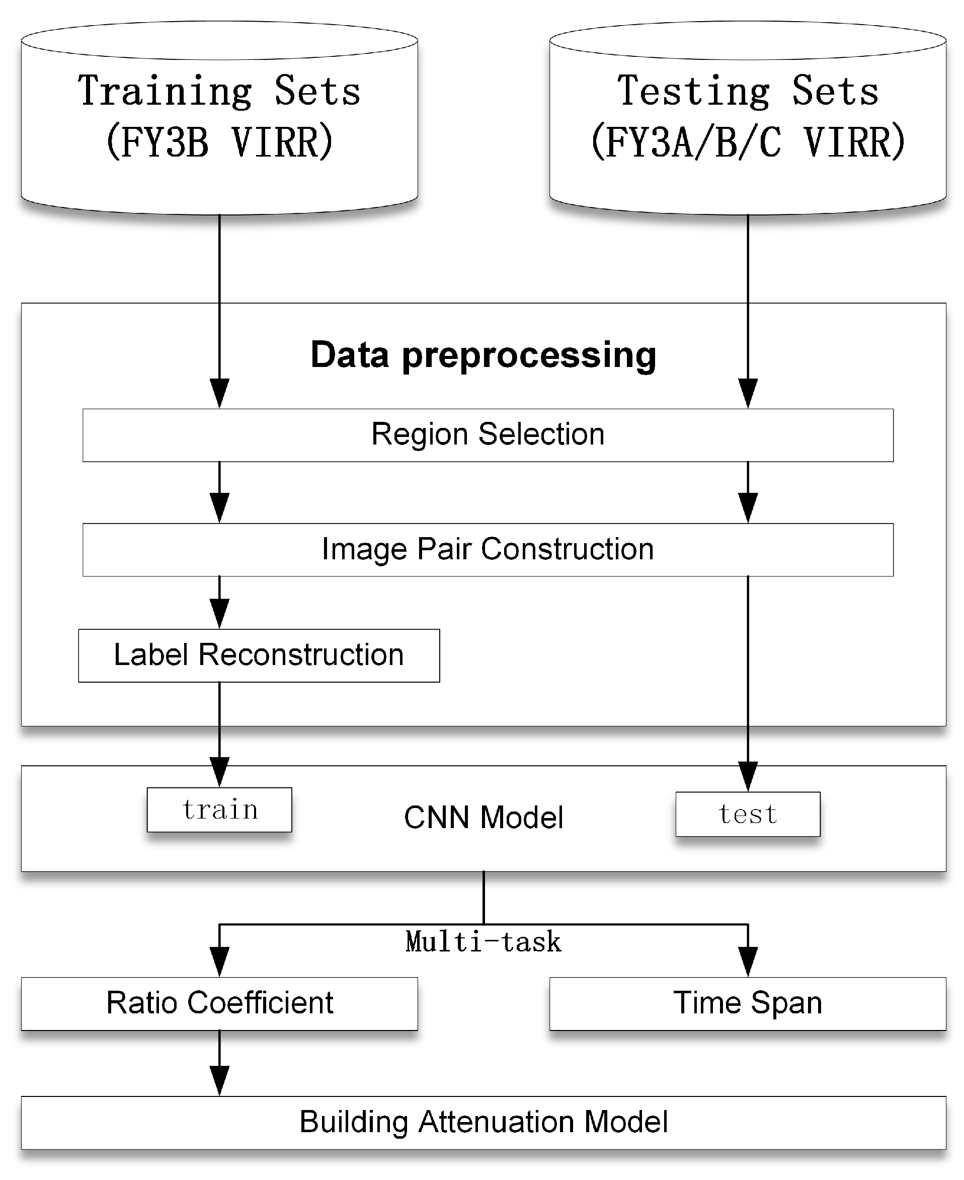
This section presents the experimental findings, providing comprehensive details on the dataset utilized and the methodology employed to construct the degradation model. Additionally, specific experimental results are presented to illustrate the analysis conducted. The basic flow of the experiment is depicted in Figure 6, outlining the sequential steps involved in the experimentation process.

4.1. Dataset and Preprocessing

This section introduces the construction and preprocessing of the dataset.

4.1.1. Dataset

In this paper, we obtained data from the VIRR sensors on the A, B and C satellites of the FengYun-3 (FY-3) series, which are part of China’s second-generation polar-orbiting meteorological satellites. The A and B satellites are the first in this series to be launched, and C is the second series. The visible and infra red radiometer (VIRR) sensor has 10 spectral channels with a 1.1 km resolution, including seven visible channels and three infrared atmospheric window channels. The specific parameters can be found in Table 2 below.

4.1.2. Region Selection

After dataset selection, regional filtering becomes imperative. Calibration necessitates detecting changes between reference and target images, which can be categorized into two types. The first type comprises normal changes in ground vegetation and landscape over time, while the second type involves degradation caused by the degradation of satellite sensors, impeding accurate reflection of ground reflectance. Calibration primarily targets the second type of change, aiming to minimize interference from the first type. Therefore, the goal of regional filtering is to select areas with minimal land cover changes, such as deserts and wastelands. In this study, the North African region was chosen as the sampling point. This selection was primarily motivated by North Africa’s prominent feature—the Sahara Desert, which is the world’s largest desert. The majority of this region experienced a tropical desert climate with minimal annual climate changes and low humidity. Additionally, the terrain is predominantly plateau, resulting in relatively stable landscape features.
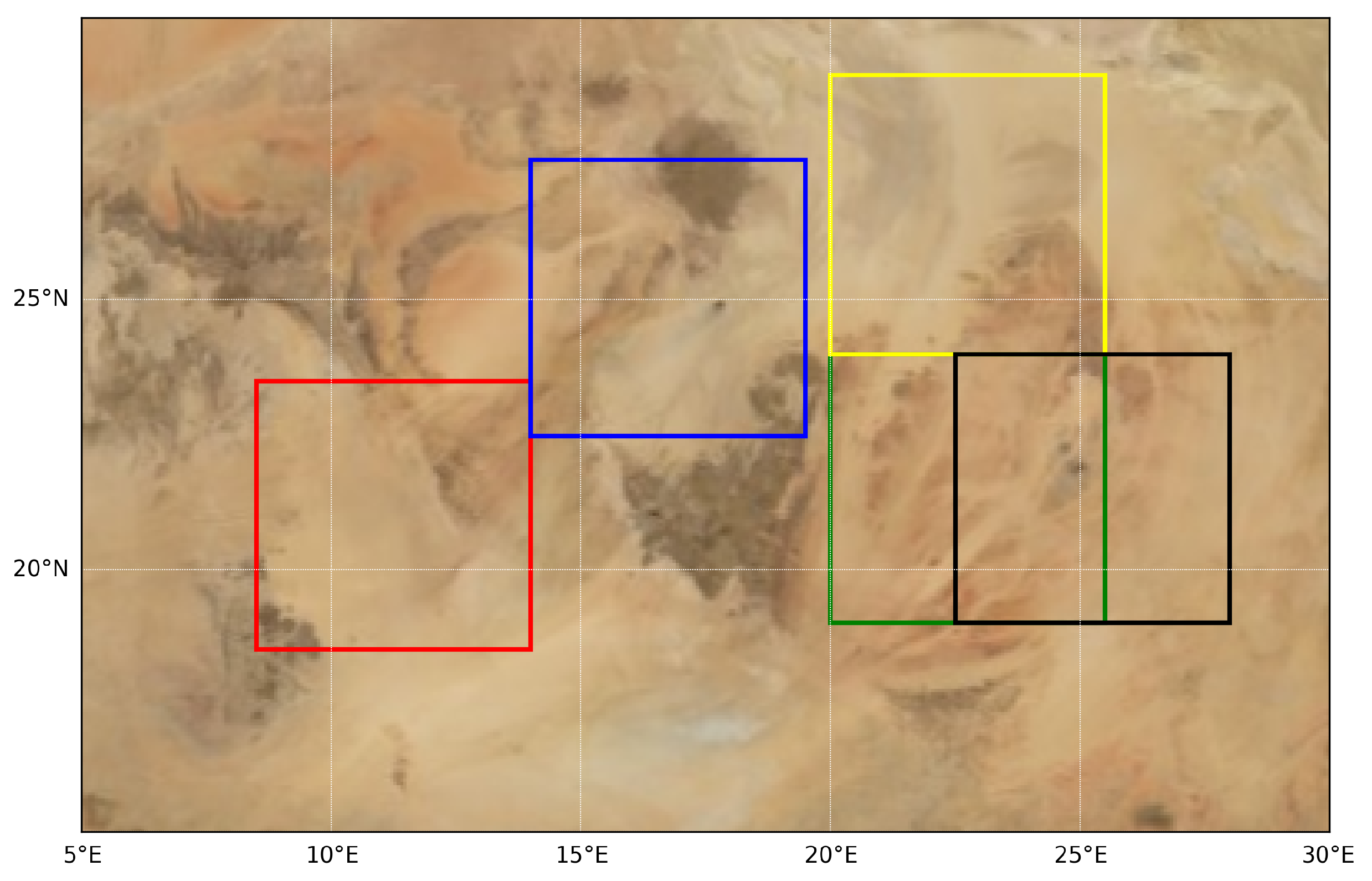
Meanwhile, to reduce computational costs and maximize training efficiency, the input image size was chosen to be 512 × 512. Therefore, further filtering of the sampling points is necessary to select the most suitable areas for calibration. We used traditional methods to detect NCPs across the entire North African region. Areas with high concentrations of NCPs were selected and divided into 512 × 512 images to form the dataset. The five selected regions are illustrated in Figure 7.
Additionally, regional selection must also consider the satellite’s view zenith angle (VZA) at the sampling points. A large VZA can result in image distortion. This distortion occurs because, as the satellite captures images from its orbit, the curvature of the Earth (being a sphere rather than a flat surface) causes images taken beyond a certain angle to become warped. Consequently, these images cannot accurately reflect the ground’s reflectance. Therefore, the training set with |VZA| ≤ 40° and the test set with |VZA| ≤ 30° were chosen for the experiments to ensure the accuracy of the test set used to construct the degradation model. Only images in which every pixel met the requisite criteria were included in the dataset. This rigorous filtering process helps guarantee the integrity and reliability of the dataset for calibration purposes. Finally, it should be noted that calibration always involves the input of two images: a reference image and a target image. Consequently, image pairs must be constructed for use in the input network. When constructing these pairs, images from different time points in the same region are selected for pairing. Additionally, the seasonal distribution has a significant impact on surface and atmospheric variations. Therefore, it is essential to select two images from the same quarter of the same or different years to eliminate the influence of seasonal factors. To guarantee the precision of the degradation model, we imposed more rigorous criteria on the test set and permit a more lenient approach to the training set. This allows for the inclusion of a greater quantity of data for training purposes, ensuring robust model development. Finally, we selected 6 years of FY3A satellite data (from 1 January 2009 to 31 December 2014), 7 years of FY3B satellite data (from 1 January 2009 to 31 December 2014) and 4 years of FY3C satellite data (from 1 January 2014 to 31 December 2017) to construct the dataset. In addition, we selected only three visible channels and three infrared channels to be used as data, striving to achieve an optimal balance between representativeness and efficiency. The specific dataset parameters are given in Table 3.
Table 3 presents the specific data parameters of the training and test sets, including the visible and infrared channels selected for different time periods. The wavelength ranges corresponding to each channel are already explained in Table 2, with each channel clearly numbered and matched accordingly. The training set comprises data from various time periods where the MST curves for these periods fit well as a linear function. In contrast, the test set includes all selected channels within the specified time period, namely, three visible and three infrared channels (1, 2, 6, 7, 8, 9). We mixed the data from all channels together to create a complete dataset, which involves different factors such as time, location and channel. Additionally, “-” indicates that the satellite is not included in the dataset. Therefore, we used FY3B as the source for the training set samples, while FY3A, FY3B and FY3C were all included in the test set for evaluation.

4.1.3. Preprocessing

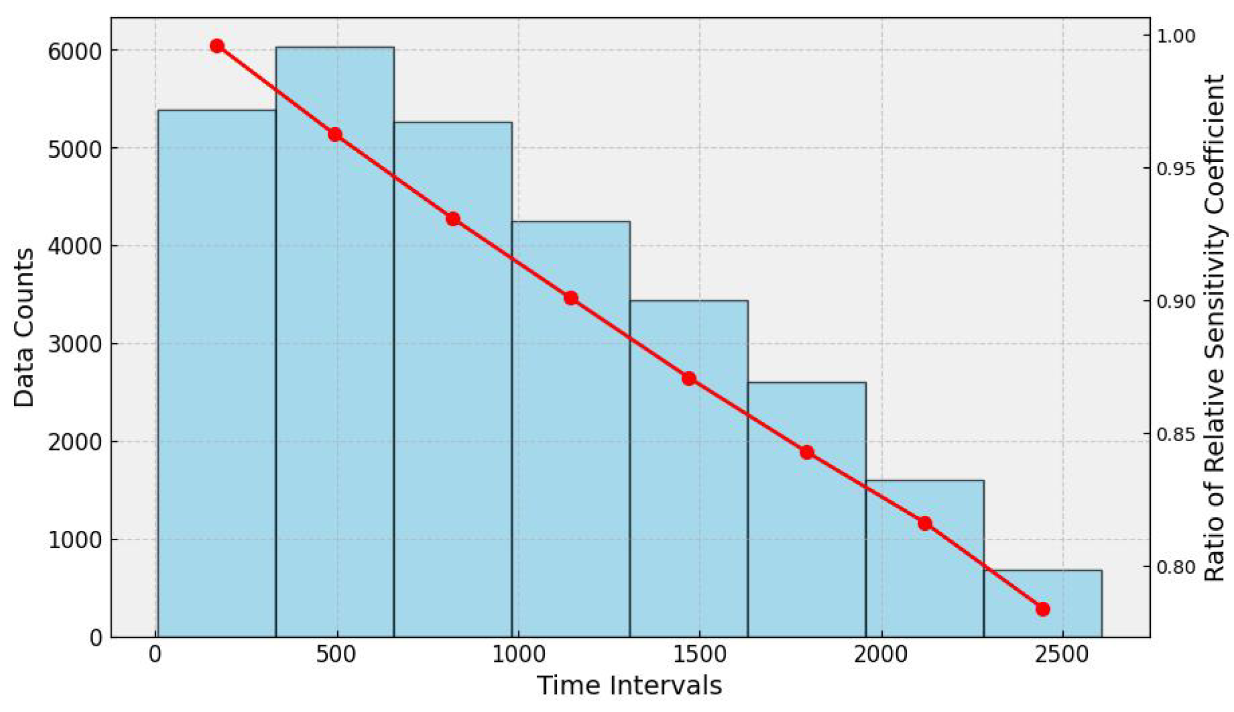
During the preprocessing stage, to augment the data and prevent model overfitting, we applied random cropping, flipping and rotation, resizing the input images to 448 × 448 pixels. Additionally, the dataset inherently exhibits data imbalance. Since the model input consists of a pair of images concatenated along the channel dimension as a single sample, constructing samples by pairing images from different time points within a given period results in more samples with short time intervals than those with long time intervals. The samples were made by choosing one image from the set as a reference and using the others as targets. We removed the original reference image from the dataset and repeated the process with the new dataset. As the new dataset became smaller, the maximum time interval for the samples became shorter, which led to data imbalance. The labels we aim to fit, m c t 1 , t 2 , are entirely dependent on the time interval between the samples. This data imbalance can significantly affect the overall dataset’s validity. For deep learning models, data imbalance might cause the model to neglect samples with fewer instances. Therefore, addressing data imbalance in the preprocessing stage is crucial. Figure 8 illustrates the extent of the data imbalance.
Therefore, we used the data label reconstruction method proposed by Xutao Li et al. to balance the data [18]. Briefly, the new label is reconstructed by multiplying an artificial coefficient around the original label m c t 1 , t 2 computation expression. This method has the advantage of artificially adjusting the label to achieve data balancing without destroying the original data information.

4.2. Construction of Degradation Models

After obtaining the relative sensitivity coefficients of the image pairs through model prediction, we further constructed an MST-like degradation model. This model consists of polynomial equations that fit the relationship between time and relative sensitivity. The basic form can be seen as follows:
S R c t , a k k = 1 N = 1 + k = 1 N a k t k
where the left side of the equation S R c t , a k k = 1 N represents the relative sensitivity coefficient calculated for channel c at time t, derived from an N-degree polynomial degradation model. The right side of the equation shows the specific calculation formula, which is essentially an N-degree polynomial equation.
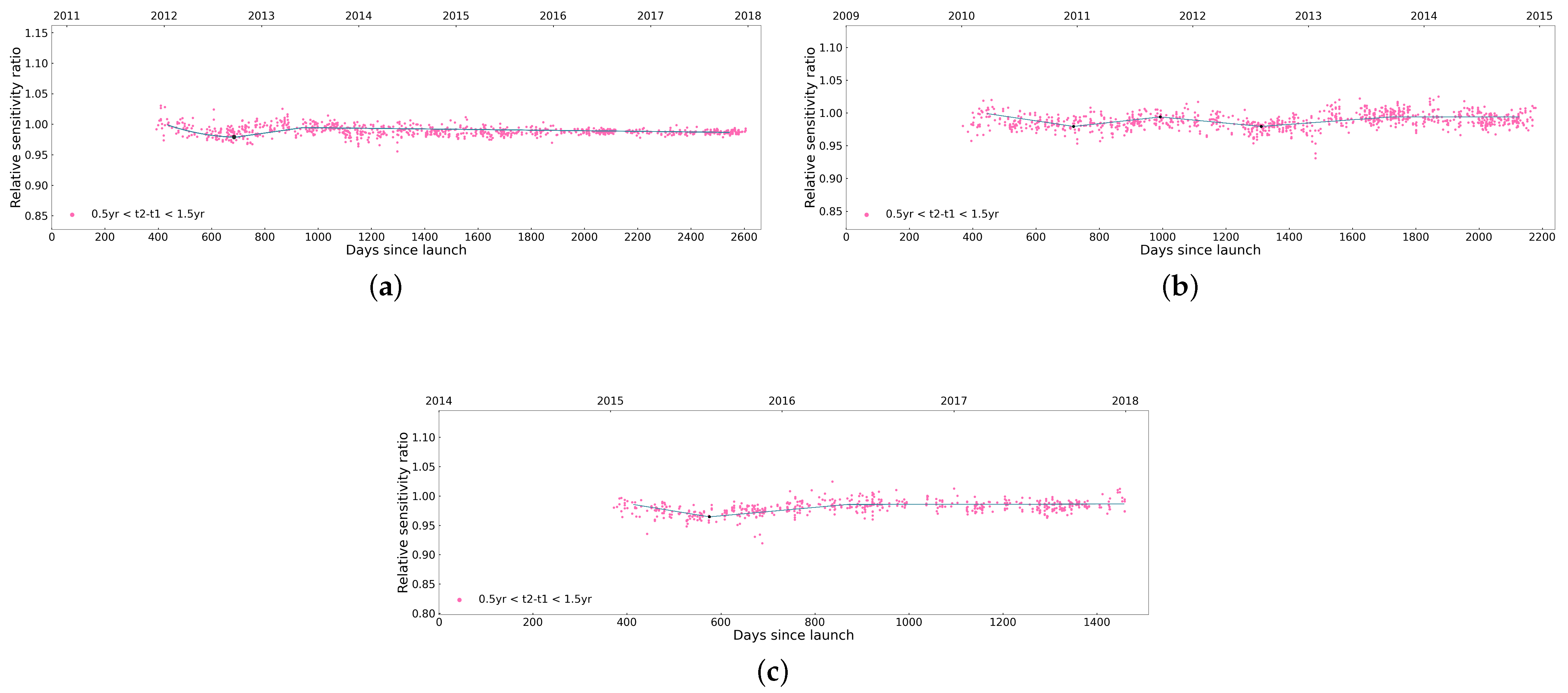
Therefore, the value of N must first be determined. Since the fitted value is m c t 1 , t 2 , a scatter plot of m c t 1 , t 2 against time is created. By observing the basic trend in the scatter plot and the distribution of the extrema, the value of N can be ascertained, because a polynomial curve with n extrema requires at least N = n + 1 . Additionally, as previously mentioned, the dataset contains more data for shorter time intervals. Hence, the scatter plot is drawn using the data from the most frequent time intervals, specifically between 0.5 years and 1.5 years. This is illustrated in Figure 9. Using this method, the polynomial degrees for the six channels of the FY3A/B/C satellites are confirmed and can be seen in Table 4.
After determining the polynomial degree, we defined an objective function and use a fitting function to derive the polynomial coefficients. Since the model outputs the ratio coefficient m c t 1 , t 2 , but the final degradation model is a polynomial equation of the relative sensitivity coefficient over time, the objective function for fitting the polynomial should aim to closely approximate these two values based on Equation (3). The objective function is defined as follows:
i = 1 M S R c t 2 i , a k k = 1 N S R c t 1 i , a k k = 1 N m c t 1 , t 2 i 2
where i denotes the i-th image pair, and M represents the total number of samples. The coefficients a k k = 1 N are the k-th order polynomial coefficients. By minimizing this objective function, we can obtain the optimal degradation model.

4.3. Results

This section primarily presents the experimental results, including the numerical display and visualization of the decay models. The polynomial coefficients derived from fitting the polynomial equations to each channel are presented in Table 5. First, we conducted an analysis of the mean, standard deviation, and coefficient of variation of these coefficients. It can be observed that the coefficients of variation for the calibration models established across the six channels of the three satellites are all below 3.5%. The ratio of the fitted values to the predicted values is close to 1. The mean ratio is approximately 1.001 and the variance remains below 0.3, demonstrating excellent modeling performance.
Moreover, Figure 10 shows the degradation curves of the six channels on the FY3A/B/C satellites using MST, IR-MAD, VGG and our method. In comparison to the absolute radiometric calibration techniques that necessitate substantial human input, our approach facilitates on-orbit automatic calibration, thereby reducing costs. In contrast to the conventional linear regression calibration methods employed in relative radiometric calibration, our method circumvents the necessity to identify NCPs, consequently diminishing the associated errors. Furthermore, in contrast to alternative deep learning techniques such as VGG-based relative radiometric calibration, our method utilizes crucial temporal information and attains superior calibration accuracy through the design of a multi-task structure. The horizontal axis represents the timeline, extending from the satellite launch time. The vertical axis represents the relative sensitivity coefficients. It can be seen that our model fits the degradation curves well, maintaining a consistent overall trend. Additionally, our method demonstrates better fitting performance in some channels compared to other methods.

4.4. Comparison with State-of-the-Art Method

To conduct horizontal comparisons with state-of-the-art (SOTA) methods, we selected the traditional calibration algorithm IR-MAD [8] and the deep-learning-based VGG algorithm [18], as both have demonstrated superior performance in calibration tasks. The evaluation metric used is the root mean square error (RMSE), a widely adopted metric for assessing model performance in fitting tasks. The RMSE is calculated as follows:
RMSE = 1 n i = 1 n y ^ ( i ) y ( i ) 1 2
where y ^ ( i ) represents the predicted value output by the model, y ( i ) represents the corresponding true value, and i denotes the i-th sample.
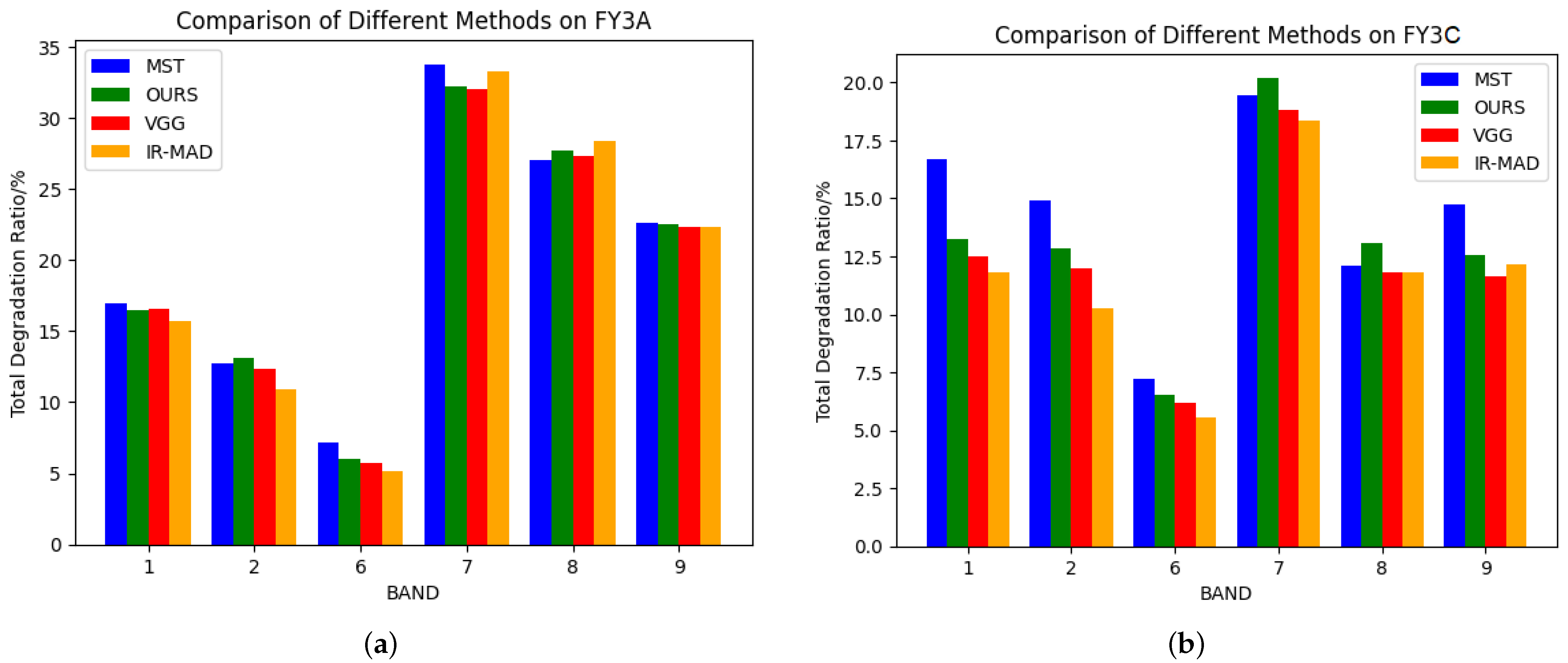
As the satellite operation time increases, the images acquired by the satellite undergo more significant changes. Therefore, to better compare the calibration effects, the total degradation rate is selected as the evaluation metric. The total degradation rate is calculated by subtracting the relative sensitivity coefficient at the end time point from that at the starting time point. Using MST as a reference, we compared the absolute error and root mean square error (RMSE) of IR-MAD, VGG and our method and present them in percentage form. Detailed results can be found in Table 6.
Our model was trained on FY3B satellite data, so choosing FY3A and FY3C for quantitative analysis helps avoid the potential overfitting issues and demonstrates the model’s generalization capability. This selection shows that our model can be applied to other satellites for calibration and achieve excellent results. As illustrated in the table, our model outperforms both the traditional IR-MAD method and the deep-learning-based VGG model, which are both considered state-of-the-art (SOTA). Our model achieves superior results across most channels, effectively demonstrating its robustness and high performance.
Figure 11 displays the total degradation rates of the six channels on FY3A/C evaluated using MST, our method, VGG and IR-MAD. This visualization offers a more intuitive representation of the consistency of the total degradation rates across different methods and demonstrates the superiority of our method over the state-of-the-art (SOTA) approaches. It can be observed that our method closely approximates the evaluation results of MST across most channels, indicating its effectiveness in capturing the overall degradation trends across the satellite channels.

4.5. Testing on Multiple Backbone

To validate the applicability of our architecture with other convolutional neural networks, we selected several classic image classification neural networks as backbones for our experiments. The experiments were limited to 300 epochs of training, and the performance of the optimal models was compared. The specific experimental results are presented in Table 7. Clearly, our model exhibits applicability across different backbones and achieves superior results compared to models lacking our framework. These findings strongly demonstrate that the time-based multi-task module enhances the neural network’s fitting of calibration coefficients. Moreover, it shows broad applicability, indicating that this framework can be directly transferred to other neural networks to improve their performance.

5. Discussion

5.1. Utilization of Temporal Information

Convolutional neural networks (CNNs) extract information by performing convolution operations on local regions, controlling the receptive field through the size and stride of the convolutional kernels. Meanwhile, the sliding window approach enables the extraction of features from the entire image. However, due to the limited size of the receptive field, CNNs cannot directly extract global information from the original image and instead rely on the stacking of network layers to expand the receptive field. When dealing with temporal information, which is not directly represented in a specific local area of the image, it becomes challenging for CNNs to extract such information directly from the feature map. Temporal information is dispersed across the feature map, and during the stacking of network layers, there is a risk of incorporating redundant information, leading to feature blurring, and the potential loss of information in deeper layers.
Therefore, directly inputting weak but crucial temporal information as features from top to bottom is overly coarse. Instead, we chose to treat it as a task, influencing the network’s bias adjustment from the bottom up during training. This approach ensures that temporal information permeates the entire network without loss and directly impacts the loss function, thereby influencing gradient updates and ensuring the network’s capability to extract temporal information.
We conducted experiments to validate this point by comparing two approaches: directly inputting temporal information as features for training and treating temporal information as a task. We selected the best results from 2000 epochs for a horizontal comparison. The specific results are summarized in Table 8. As shown, both methods achieved excellent performance on the test sets from the FY3A/C satellites, surpassing the VGG network without temporal information (see Table 6). Moreover, training with temporal information as a task outperformed training with temporal information as features in most channels and overall RMSE, demonstrating the effectiveness of multi-task training.

5.2. Ablation Study

To further validate the effectiveness of the multi-task module based on temporal information, we conducted an ablation study to evaluate the results. Considering fairness, the experiments were configured to train for 2000 epochs, allowing for full convergence before selecting the optimal model for horizontal comparison. The results are presented in Table 9. Evidently, models that did not use our framework performed significantly worse on the FY3A/C test sets compared to those using our framework. Not only did they lag substantially in most channels but the overall RMSE evaluation also showed a difference of 30.4% for FY3A and 13.3% for FY3C.

6. Conclusions

This paper introduces a novel approach: a multi-task convolutional neural network framework leveraging temporal information for calibration. Notably, this method stands out as the first to underscore the significance of temporal information in deep-learning-based relative radiometric calibration methods. It introduces a multi-task structure, treating temporal information as a task to enhance calibration. Experiments and comparisons with state-of-the-art (SOTA) methods demonstrate its superior performance and effectiveness. Moreover, by substituting the backbone, we demonstrated its broad applicability to various convolutional neural network calibration methods. Finally, we have examined the efficiency of the framework in extracting temporal information for calibration. In the future, we will continue to explore the integration of information between different channels and develop multi-channel calibration within a time-based multi-task module. Furthermore, we plan to employ transfer learning to develop a unified calibration model across multiple sensors and channels, thereby overcoming the limitation of requiring retraining for different sensors.

Author Contributions

Conceptualization, L.T. and X.Z.; Methodology, L.T.; Software, L.T.; Validation, L.T., C.L. and M.L.; Formal analysis, L.T.; Investigation, X.Z.; Resources, X.H.; Data curation, X.H.; Writing—original draft, L.T., C.L. and M.L.; Writing—review & editing, X.Z., C.L. and M.L.; Visualization, X.H.; Supervision, X.Z., C.L. and M.L.; Project administration, X.Z. All authors have read and agreed to the published version of the manuscript.

Funding

This work was supported by the Nature Science Program of Shenzhen under Grant JCYJ20210324120208022 and the Major Project of High Resolution Earth Observation System under Grant 30-Y60B01-9003-22/23.

Data Availability Statement

The data presented in this study are available on request from the corresponding author, because the data are not publicly available due to privacy or ethical restrictions.

Conflicts of Interest

The authors declare no conflicts of interest.

References

  1. Teillet, P.M.; Slater, P.N.; Ding, Y.; Santer, R.P.; Jackson, R.D.; Moran, M.S. Three methods for the absolute calibration of the NOAA AVHRR sensors in-flight. Remote Sens. Environ. 1990, 31, 105–120. [Google Scholar] [CrossRef]
  2. Chen, Y.; Sun, K.; Li, W.; Hu, X.; Li, P.; Bai, T. Vicarious Calibration of FengYun-3D MERSI-II at Railroad Valley Playa Site: A Case for Sensors with Large View Angles. Remote Sens. 2021, 13, 1347. [Google Scholar] [CrossRef]
  3. Rudolf, D.; Raab, S.; Döring, B.J.; Jirousek, M.; Reimann, J.; Schwerdt, M. Absolute radiometric calibration of the novel DLR “Kalibri” transponder. In Proceedings of the German Microwave Conference, Nuremberg, Germany, 16–18 March 2015; pp. 323–326. [Google Scholar]
  4. Dinguirard, M.; Slater, P.N. Calibration of space-multispectral imaging sensors: A review. Remote Sens. Environ. 1999, 68, 194–205. [Google Scholar] [CrossRef]
  5. Yuan, D.; Elvidge, C.D. Comparison of relative radiometric normalization techniques. ISPRS J. Photogramm. Remote Sens. 1996, 51, 117–126. [Google Scholar] [CrossRef]
  6. Schott, J.R.; Salvaggio, C.; Volchok, W.J. Radiometric scene normalization using pseudoinvariant features. Remote Sens. Environ. 1988, 26, 1–16. [Google Scholar] [CrossRef]
  7. Nielsen, A.A.; Conradsen, K.; Simpson, J.J. Multivariate Alteration Detection (MAD) and MAF Postprocessing in Multispectral, Bitemporal Image Data: New Approaches to Change Detection Studies. Remote Sens. Environ. 1998, 64, 1–19. [Google Scholar] [CrossRef]
  8. Nielsen, A.A. The Regularized Iteratively Reweighted MAD Method for Change Detection in Multi- and Hyperspectral Data. IEEE Trans. Image Process. Publ. IEEE Signal Process. Soc. 2007, 16, 463–478. [Google Scholar] [CrossRef] [PubMed]
  9. Yang, X.; Lo, C.P. Relative radiometric normalization performance for change detection from multi-date satellite images. Photogramm. Eng. Remote Sens. 2000, 66, 967–980. [Google Scholar]
  10. Hall, F.G.; Strebel, D.E.; Nickeson, J.E.; Goetz, S.J. Radiometric rectification: Toward a common radiometric response among multidate, multisensor images. Remote Sens. Environ. 1991, 35, 11–27. [Google Scholar] [CrossRef]
  11. Elvidge, C.D.; Yuan, D.; Weerackoon, R.D.; Lunetta, R.S. Relative radiometric normalization of Landsat multispectral scanner (MSS) data using an automatic scattergram-controlled regression. Photogramm. Eng. Remote Sens. 1995, 61, 1255–1260. [Google Scholar]
  12. Velloso, M.L.F.; de Souza, F.J.; Simoes, M. Improved radiometric normalization for land cover change detection: An automated relative correction with artificial neural network. IEEE Int. Geosci. Remote Sens. Symp. 2002, 6, 3435–3437. [Google Scholar]
  13. Yang, G.; Pu, R.; Huang, W.; Wang, J.; Zhao, C. A Novel Method to Estimate Subpixel Temperature by Fusing Solar-Reflective and Thermal-Infrared Remote-Sensing Data With an Artificial Neural Network. IEEE Trans. Geosci. Remote Sens. 2010, 48, 2170–2178. [Google Scholar] [CrossRef]
  14. LeCun, Y.; Bottou, L.; Bengio, Y.; Haffner, P. Gradient-based learning applied to document recognition. Proc. IEEE 1998, 86, 2278–2324. [Google Scholar] [CrossRef]
  15. Xing, F.; An, R.; Guo, X.; Shen, X. Mapping the Continuous Cover of Invasive Noxious Weed Species Using Sentinel-2 Imagery and a Novel Convolutional Neural Regression Network. Remote Sens. 2024, 16, 1648. [Google Scholar] [CrossRef]
  16. Li, Z.; Wei, D.; Zhang, X.; Gao, Y.; Zhang, D. A Daily High-Resolution Sea Surface Temperature Reconstruction Using an I-DINCAE and DNN Model Based on FY-3C Thermal Infrared Data. Remote Sens. 2024, 16, 1745. [Google Scholar] [CrossRef]
  17. Xie, Y.; Meng, X.; Wang, J.; Li, H.; Lu, X.; Ding, J.; Jia, Y.; Yang, Y. Enhancing GNSS Deformation Monitoring Forecasting with a Combined VMD-CNN-LSTM Deep Learning Model. Remote Sens. 2024, 16, 1767. [Google Scholar] [CrossRef]
  18. Li, X.; Ye, Z.; Ye, Y.; Hu, X. A Convolutional Neural Network-Based Relative Radiometric Calibration Method. IEEE Trans. Geosci. Remote Sens. 2021, 60, 5403611. [Google Scholar] [CrossRef]
  19. Wang, L.; Hu, X.; Chen, L.; He, L. Consistent calibration of VIRR reflective solar channels onboard FY-3A, FY-3B, and FY-3C using a multisite calibration method. Remote Sens. 2018, 10, 1336. [Google Scholar] [CrossRef]
  20. Simonyan, K.; Zisserman, A. Very deep convolutional networks for large-scale image recognition. arXiv 2014, arXiv:1409.1556. [Google Scholar]
  21. Bolei, Z.; Aditya, K.; Agata, L.; Aude, O.; Antonio, T. Learning Deep Features for Discriminative Localization. In Proceedings of the IEEE Conference on Computer Vision and Pattern Recognition (CVPR), Las Vegas, NV, USA, 27–30 June 2016; pp. 2921–2929. [Google Scholar]
  22. Tang, H.; Liu, J.; Zhao, M.; Gong, X. Progressive Layered Extraction (PLE): A Novel Multi-Task Learning (MTL) Model for Personalized Recommendations. In Proceedings of the 14th ACM Conference on Recommender Systems (RecSys ’20), Virtual, 22–26 September 2020; Association for Computing Machinery: New York, NY, USA, 2020; pp. 269–278. [Google Scholar]
Figure 1. This figure shows the visualization of the calibration, where the upper half of the figure shows an image from 27 May 2009 on channel 1 of FY3A, and the lower half shows an image from 25 June 2014 on channel 1 of FY3A. They all situate between 18.8°N and 23.5°N latitude and 22.5°E and 27.5°E longitude. The processing in the lower half of the figure is (a) without calibration, (b) with MST calibration, (c) with IR-MAD calibration, (d) with VGG network calibration and (e) with our calibration method.
Remotesensing 16 03346 g001
Figure 2. Multi-task convolutional neural network model based on temporal information.
Remotesensing 16 03346 g002
Figure 3. Feature Extraction Module.
Remotesensing 16 03346 g003
Figure 4. Multi-task module.
Remotesensing 16 03346 g004
Figure 5. The multisite (MST) calibration results on (a) FY3A, (b) FY3B and (c) FY3C for six selected channels. Different colors for different channels. This shows that the relative sensitivity coefficients of each channel decrease with time.
Remotesensing 16 03346 g005
Figure 6. The experimental procedure.
Remotesensing 16 03346 g006
Figure 7. The illustration of the five regions of North Africa where NCPs are concentrated, each cut in a 512 × 512 square.
Remotesensing 16 03346 g007
Figure 8. The presentation of data imbalance. The x-axis represents the time intervals between the reference and target images. The left vertical axis (y-axis of the histogram) represents the number of image pairs at different time intervals. The right vertical axis (y-axis of the line graph) represents the relative sensitivity coefficient m c t 1 , t 2 for different time intervals. This illustrates that as the time interval increases and the number of pairs in the dataset decreases, the labeled value of m c t 1 , t 2 also decreases.
Remotesensing 16 03346 g008
Figure 9. The scatter plots showing the variation in the relative sensitivity ratio m c t 1 , t 2 with respect to Days. Since Launch for image pairs with time intervals between 0.5 years and 1.5 years for channel 6 on the FY3A (a), FY3B (b) and FY3C (c) satellites. By observing the number of extrema in the basic trend, we can determine the degree of the fitting polynomial. For instance, in (a), there is 1 extremum point, so the polynomial degree for fitting channel 6 on FY3A is N = 2 . Similarly, in (b), there are 3 extrema points, resulting in a polynomial degree of N = 4 for FY3B, and there is 1 extremum point in (c), so the polynomial degree of FY3C is N = 2 .
Remotesensing 16 03346 g009
Figure 10. The sensitivity degradation curves for channels 1, 2, 6, 7, 8 and 9 on the (a) FY3A VIRR, (b) FY3B VIRR and (c) FY3C VIRR satellites using MST, IRMAD, VGG and our method.
Remotesensing 16 03346 g010aRemotesensing 16 03346 g010b
Figure 11. The total degradation ratio for channels 1, 2, 6, 7, 8 and 9 on the (a) FY3A VIRR and (b) FY3C VIRR satellites using MST, IRMAD, VGG, and our method.
Remotesensing 16 03346 g011
Table 1. Parameter Setting on the Feature Extraction Module.
Configuration
15 weight layers
input (448 × 448 image pair)
LayersOutput SizeParameters
Convolution Block 1448 × 448[3 × 3 conv, 16 channels, 1 stride] × 2
Transition Layer224 × 224[2 × 2 average pool, 2 stride]
Convolution Block 2224 × 224[3 × 3 conv, 32 channels, 1 stride] × 2
Transition Layer112 × 112[2 × 2 average pool, 2 stride]
Convolution Block 3112 × 112[3 × 3 conv, 64 channels, 1 stride] × 2
Transition Layer56 × 56[2 × 2 average pool, 2 stride]
Convolution Block 456 × 56[3 × 3 conv, 128 channels, 1 stride] × 2
Transition Layer28 × 28[2 × 2 average pool, 2 stride]
Convolution Block 528 × 28[3 × 3 conv, 128 channels, 1 stride] × 2
Transition Layer14 × 14[2 × 2 average pool, 2 stride]
Convolution Block 614 × 14[3 × 3 conv, 128 channels, 1 stride] × 2
Transition Layer7 × 7[2 × 2 average pool, 2 stride]
Table 2. Specifications of FY-3 (A/B/C)/VIRR spectral band.
Band12345678910
Central
Wavelength0.4550.5050.5550.6300.8651.3601.6003.74010.8012.00
(µm)
Band
Range0.43–0.480.43–0.480.53–0.580.58–0.680.84–0.891.325–1.3951.55–1.643.55–3.9310.3–11.311.5–12.5
(µm)
Noise ( Δ ρ
or   Δ K )0.05%0.05%0.05%0.1%0.1%0.19%0.15%0.3 K (FY-3A 0.4 K)0.2 K0.2 K
(300 K)
Dynamic
Range0–50%0–50%0–50%0–100%0–100%0–90%0–90%180–350 K180–350 K180–350 K
( ρ /K)
Table 3. Summary of Our Dataset.
Training SetsTest Sets
FY3A VIRR-20090101–20141231
FY3B VIRR20150101–20171231(1,2,6)20101119–20171231
20130101–20151231(7,8,9)
FY3C VIRR-20140101–20171231
|VZA|≤40°≤30°
Interval [ 365.25 × y 1 40 , 365.25 × y 1 + 40 ] [ 365.25 × y 2 30 , 365.25 × y 2 + 30 ]
Table 4. Polynomial Degree of Different Bands and Satellite.
BandFY3A VIRRFY3B VIRRFY3C VIRR
1442
2442
6242
7442
8242
9242
Table 5. Calibration Model Coefficients for FY3A/B/C VIRR Sensors.
SensorBanda1a2a3a4MeanStdCV ( μ / σ , % )
FY3A VIRR1 1.98 × 10 4 9.48 × 10 8 2.76 × 10 11 3.04 × 10 15 1.0010.0151.536
2 2.01 × 10 4 1.18 × 10 7 3.17 × 10 11 2.48 × 10 15 1.0020.0292.935
6 4.32 × 10 5 6.28 × 10 9 --1.0010.0111.100
7 4.39 × 10 4 5.15 × 10 8 7.28 × 10 11 2.28 × 10 14 1.0010.0313.142
8 2.47 × 10 4 3.28 × 10 8 --1.0020.0272.725
9 1.34 × 10 4 5.84 × 10 10 --1.0010.0112.187
FY3B VIRR1 3.58 × 10 4 3.11 × 10 7 1.37 × 10 10 2.07 × 10 14 1.0010.0121.193
2 2.79 × 10 4 2.78 × 10 7 1.32 × 10 10 2.10 × 10 14 1.0010.0242.380
6 9.12 × 10 6 3.14 × 10 8 1.09 × 10 11 1.36 × 10 15 1.0000.0090.854
7 1.80 × 10 4 1.61 × 10 7 8.44 × 10 11 1.06 × 10 14 1.0010.0222.213
8 1.59 × 10 4 3.01 × 10 8 3.43 × 10 11 9.12 × 10 15 1.0010.0201.956
9 3.22 × 10 4 2.49 × 10 7 1.14 × 10 10 1.73 × 10 14 1.0000.0141.415
FY3C VIRR1 1.73 × 10 4 4.72 × 10 8 --1.0010.0151.522
2 1.58 × 10 4 3.89 × 10 8 --1.0020.0282.767
6 6.71 × 10 5 1.33 × 10 8 --1.0010.0101.045
7 2.72 × 10 4 6.75 × 10 8 --1.0010.0343.426
8 1.68 × 10 4 4.44 × 10 8 --1.0010.2972.969
9 1.64 × 10 4 4.50 × 10 8 --1.0000.0232.300
Table 6. Total degradation (absolute difference to MST) for FY3A/C VIRR sensors. The bolded numbers in the table represent the values with the best vertical comparison performance.
SensorMethodTotal Degradation (Absolute Difference to MST)/%
Band 1Band 2Band 6Band 7Band 8Band 9RMSE
FY3A VIRRMST16.96(-)12.74(-)7.18(-)33.77(-)26.98(-)22.61(-)-
IR-MAD15.73(1.24)10.94(1.80)5.18(2.00)33.22(0.55)28.37(1.40)22.31(0.30)1.39
VGG16.57(0.40)12.33(0.41)5.73(1.45)32.06(1.71)27.30(0.32)22.31(0.30)0.96
Ours16.51(0.45)13.12(0.38)6.06(1.11)32.24(1.53)27.74(0.77)22.53(0.08)0.87
FY3C VIRRMST16.69(-)14.89(-)7.24(-)19.47(-)12.10(-)14.73(-)-
IR-MAD11.83(4.86)10.26(4.63)5.53(1.71)18.33(1.14)11.84(0.26)12.18(2.55)3.05
VGG12.48(4.23)12.00(2.89)6.16(1.08)18.83(0.64)11.79(0.31)11.65(3.08)2.50
Ours13.23(3.46)12.82(2.07)6.52(0.72)20.21(0.74)13.06(0.95)12.58(2.15)1.95
Table 7. Total degradation (absolute difference to MST) for different backbones on FY3A/CVIRR sensors. The bolded numbers in the table represent the values with the best vertical comparison performance.
SensorMethodTotal Degradation (Absolute Difference to MST)/%
Band 1Band 2Band 6Band 7Band 8Band 9RMSE
FY3A VIRRMST16.96(-)12.74(-)7.18(-)33.77(-)26.98(-)22.61(-)-
mobilenet17.51(0.55)14.08(1.34)5.64(1.54)31.70(2.07)27.30(0.32)22.19(0.42)1.23
mobilenet Task17.63(0.67)13.52(0.79)5.87(1.31)32.16(1.61)27.79(0.81)22.79(0.18)1.01
mobilenetV216.87(0.10)13.81(1.07)5.82(1.35)31.04(2.73)26.57(0.41)21.96(0.65)1.59
mobilenetV2 Task16.62(0.35)13.19(0.46)6.20(0.98)31.13(2.64)26.72(0.26)22.34(0.27)1.18
squeezenet17.73(0.77)14.25(1.51)5.99(1.19)30.98(2.79)26.80(0.18)22.06(0.55)1.44
squeezenet Task17.97(1.01)14.06(1.32)6.52(0.66)32.17(1.60)27.88(0.90)22.91(0.30)1.05
preactresnet16.05(0.91)12.05(0.68)5.70(1.48)30.98(2.79)26.26(0.72)21.57(1.04)1.46
preactresnet Task17.23(0.27)13.51(0.78)5.48(1.70)32.10(1.67)26.84(0.14)22.49(0.12)1.03
FY3C VIRRMST16.69(-)14.89(-)7.24(-)19.47(-)12.10(-)14.73(-)-
mobilenet12.77(3.92)11.82(3.07)5.96(1.28)19.69(0.22)13.61(1.50)12.89(1.84)2.31
mobilenet Task13.50(3.19)12.05(2.84)6.02(1.22)20.25(0.78)14.03(1.92)13.44(1.30)2.07
mobilenetV213.17(3.52)12.03(2.86)5.30(1.94)20.44(0.97)14.57(2.46)14.28(0.45)2.15
mobilenetV2 Task13.29(3.39)12.60(2.29)6.35(0.89)20.61(1.14)13.51(1.41)13.04(1.69)1.99
squeezenet11.99(4.70)11.60(3.29)5.54(1.70)19.47(0.002)13.07(0.97)12.13(2.60)2.69
squeezenet Task13.74(2.94)12.36(2.53)5.95(1.29)20.89(1.42)14.81(2.70)14.38(0.36)2.09
preactresnet12.81(3.88)11.82(3.07)6.01(1.23)20.57(1.10)13.63(1.52)13.13(1.60)2.31
preactresnet Task13.39(3.30)12.49(2.40)5.71(1.53)20.93(1.47)13.82(1.72)13.27(1.46)2.09
Table 8. Comparison of the total degradation rate, absolute error and RMSE between the use of time as a feature for training and the use of time as a task for training for six channels on FY3A/C VIRR sensors. The bolded numbers in the table represent the values with the best vertical comparison performance.
SensorMethodTotal Degradation (Absolute Difference to MST)/%
Band 1Band 2Band 6Band 7Band 8Band 9RMSE
FY3A VIRRMST16.96(-)12.74(-)7.18(-)33.77(-)26.98(-)22.61(-)-
Train as feature17.41(0.44)14.35(1.61)5.77(1.40)33.16(0.61)28.74(1.77)23.23(0.62)1.20
Train as task16.51(0.45)13.12(0.38)6.06(1.11)32.24(1.53)27.74(0.77)22.53(0.08)0.87
FY3C VIRRMST16.69(-)14.89(-)7.24(-)19.47(-)12.10(-)14.73(-)-
Train as feature13.39(3.30)12.80(2.09)6.01(1.22)20.55(1.08)13.16(1.06)12.52(2.21)2.00
Train as task13.23(3.46)12.82(2.07)6.52(0.72)20.21(0.74)13.06(0.95)12.58(2.15)1.95
Table 9. Comparison of the total degradation rate, absolute error and RMSE between model without our framework and model with our framework for six channels on FY3A/C VIRR sensors. The bolded numbers in the table represent the values with the best vertical comparison performance.
SensorMethodTotal Degradation (Absolute Difference to MST)/%
Band 1Band 2Band 6Band 7Band 8Band 9RMSE
FY3A VIRRMST16.96(-)12.74(-)7.18(-)33.77(-)26.98(-)22.61(-)-
Train without framework16.28(0.68)12.15(0.59)5.16(2.02)31.71(2.05)27.10(0.12)22.16(0.45)1.25
Train with framework16.51(0.45)13.12(0.38)6.06(1.11)32.24(1.53)27.74(0.77)22.53(0.08)0.87
FY3C VIRRMST16.69(-)14.89(-)7.24(-)19.47(-)12.10(-)14.73(-)-
Train without framework12.79(3.89)12.65(2.24)5.96(1.28)19.30(0.16)11.97(0.13)11.79(2.94)2.25
Train with framework13.23(3.46)12.82(2.07)6.52(0.72)20.21(0.74)13.06(0.95)12.58(2.15)1.95
Disclaimer/Publisher’s Note: The statements, opinions and data contained in all publications are solely those of the individual author(s) and contributor(s) and not of MDPI and/or the editor(s). MDPI and/or the editor(s) disclaim responsibility for any injury to people or property resulting from any ideas, methods, instructions or products referred to in the content.