1. Introduction
With the rapid development of sensor technology, multisensor mapping platforms are becoming increasingly popular in geospatial data acquisitions. Light detection and ranging (LiDAR) scanners and cameras are integrated on common platforms (i.e., rigid installations), where the relative orientation and position between the instruments are constant within the platform frame. The increased use of multisensor mapping platforms has been facilitated by the smaller sensor form factor, lower cost, and increased accuracy. Furthermore, this has enabled data fusion of different complementary data sources. Weight limitations inherent to unmanned aerial vehicles (UAVs) used to restrain their payloads in the early days of UAV development. At present, UAVs built for mapping purposes are commonly equipped with several sensors such as LiDAR scanners, cameras, and global navigation satellite system (GNSS)-aided inertial navigation systems (INS), e.g., [
1,
2,
3]. Hyperspectral imaging (HSI) cameras have also been integrated on GNSS/INS-supported UAVs together with LiDAR scanners, e.g., [
4], and similar set-ups are used for mapping from helicopters and airplanes, e.g., [
5,
6].
The data from the different sensors have different strengths that are utilized in the data analysis. One example is the unique potential for detailed radiometric analyses using HSI. Some examples of the applications of HSI include geological mapping, e.g., [
7,
8], forestry, e.g., [
9,
10], urban classification, e.g., [
6,
11], and agriculture, e.g., [
12]. HSI cameras are often LP cameras, as one image dimension is used for signal registration in multiple spectral bands. After data acquisition, the appropriate geospatial accuracy of the data from the different sensors is traditionally obtained and documented from fundamentally different processing pipelines. Geometric errors may introduce both systematic and random errors in the data to be analyzed. Enhanced geometric accuracy thus increases the value of the acquired data and allows more advanced analysis techniques to be applied, including temporal studies from recurring data acquisitions. Images are commonly aligned in the bundle adjustment, while LiDAR point clouds are separately matched in a strip adjustment process to provide accurate estimates of the interior and exterior parameters of the respective sensors. Bundle adjustment traditionally discretizes the trajectory parameters as the exterior orientations of the camera per image exposure, while the LiDAR strip adjustment discretizes the trajectory corrections in temporally longer strips. However, if mounted on the same platform, the observations from these sensors conceptually provide information for estimating common trajectory parameters (i.e., the GNSS/INS position and orientation errors). Due to the sensor-specific trajectory error parameterization, the common trajectory parameters cannot be readily estimated based on observation residuals from the different functional models.
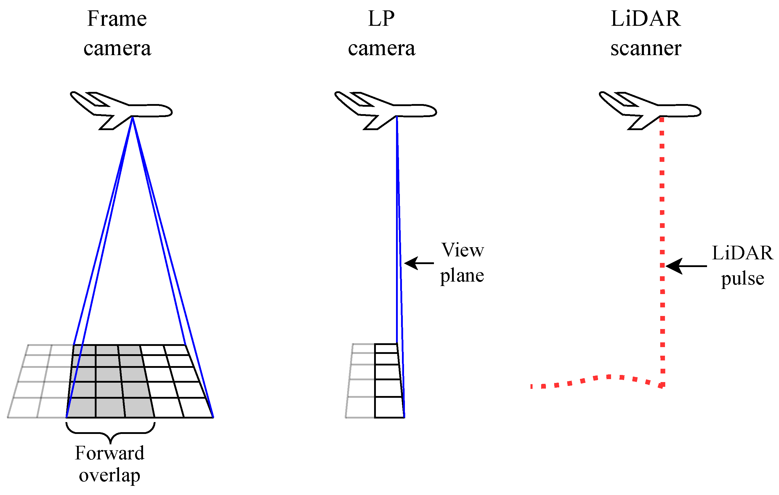
The operating principles of frame cameras, linear pushbroom (LP) cameras, and LiDAR scanners are shown in
Figure 1. The passive cameras store radiometric information in image pixels. Forward overlap, commonly seen in photogrammetric blocks from frame images, is not feasible to achieve with LP image lines without unwanted distortion. The active LiDAR scanner measures the range and angle of the emitted pulses. Based on the scanner-specific configuration and technology, forward overlap may also be achieved in LiDAR scanning. This could be accomplished, for example, using rotating mirrors or prisms.
Here, we present a novel theoretical development for integrating observations from 3D LiDAR point clouds, 2D images from frame cameras, and 1D image lines from LP cameras in a joint hybrid adjustment using one common trajectory correction model for all observation types. This modeling allows integrating the data from the three sensor types at the observation level such that the optimal matching solution from all the data is found. To our knowledge, this is the first demonstration of a joint adjustment involving these three sensor modalities using a rigorous and scalable trajectory formulation.
3. Methodology
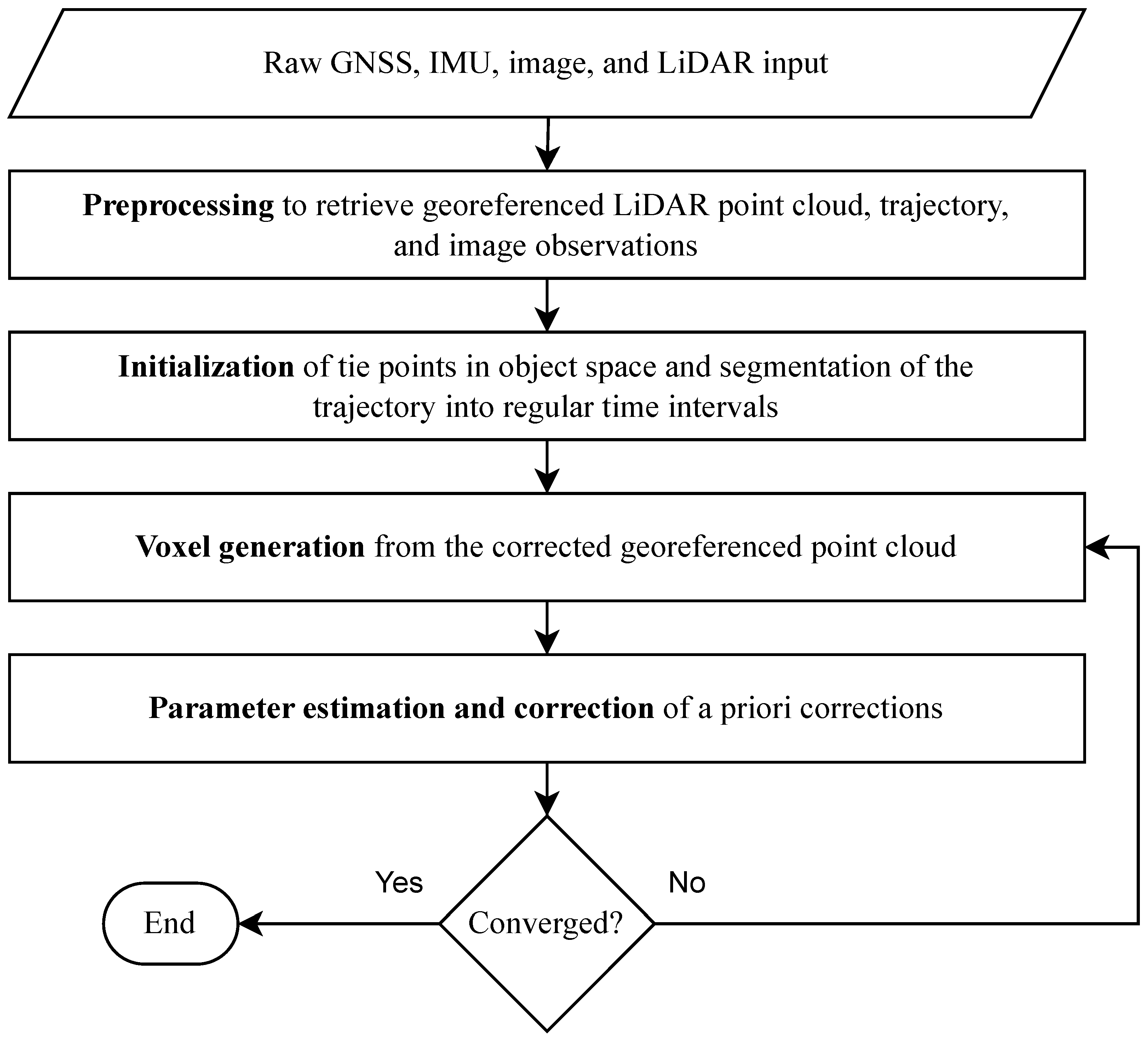
Figure 2 shows the workflow where the method is divided into four simplified steps.
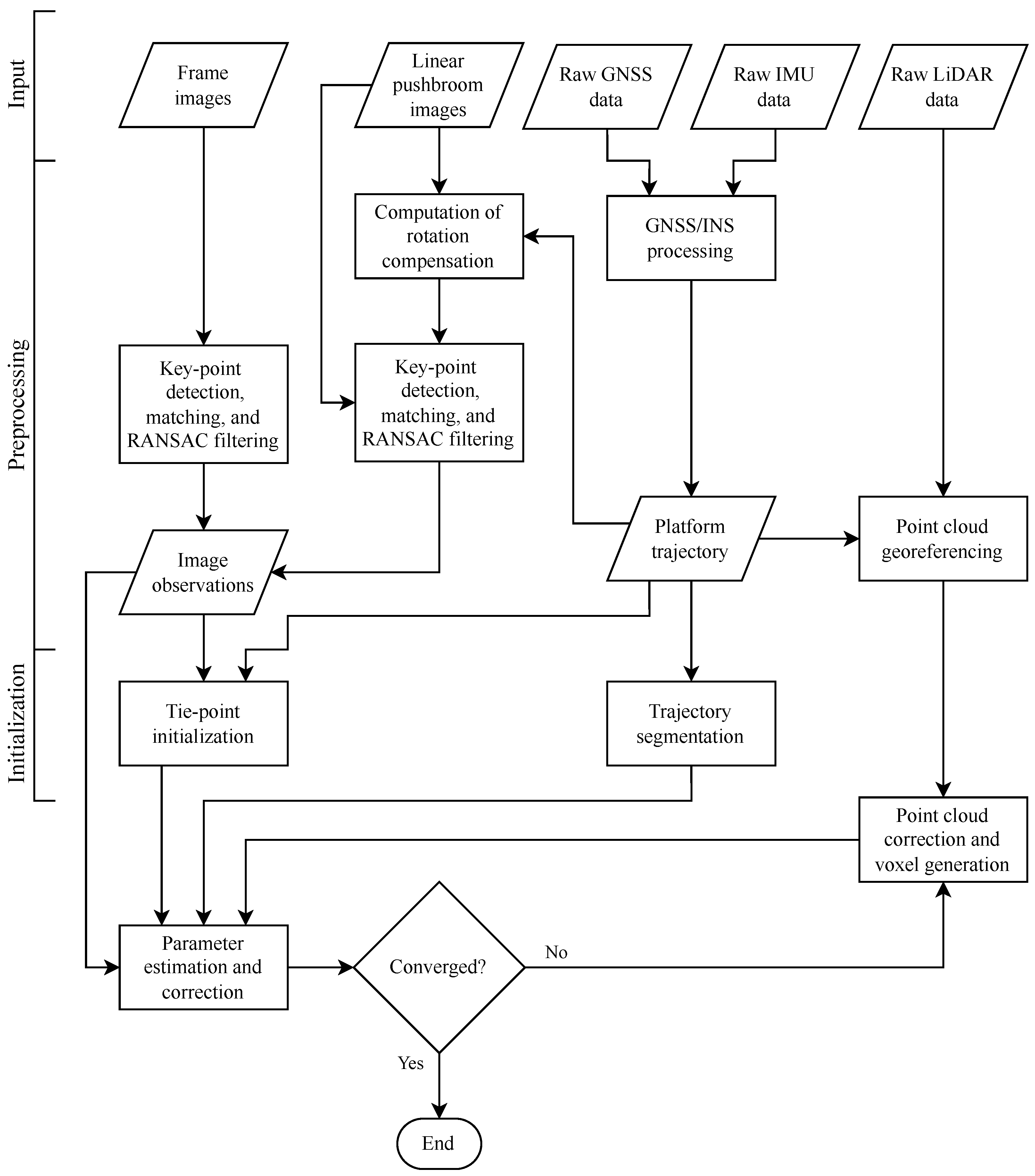
Figure 3 shows the steps in more detail. More detailed explanations of the steps in
Figure 3 can be found in [
13,
14]. Thus, only the basic underlying theory is covered in this section.
3.1. Preprocessing
The preprocessing steps are needed to retrieve the observations from frame images and LP image lines before the adjustment. Additionally, the platform trajectory is computed, and point clouds are formed from the direct georeferencing of LiDAR points.
3.1.1. GNSS/INS Processing
A Kalman filter/smoother is used to retrieve the trajectory of the platform using the software TerraPos; see [
25]. The trajectory consists of high-rate positions and orientations for the platform, along with their full covariance matrices. To conduct the GNSS/INS processing as presented, an IMU must be rigidly mounted on each platform, and the lever arm between the GNSS antenna and an IMU is either known a priori or estimated using the Kalman filter. Typically, a gyro-stabilized mount serves as a platform within an aircraft.
3.1.2. Point Cloud Georeferencing
Once an initial trajectory has been computed via the Kalman filter, it is used for the direct georeferencing of the LiDAR measurements with the use of the a priori mounting parameters and raw LiDAR scanner measurements. The result of this is a georeferenced point cloud with spatial mismatches between the overlapping scans owing to scanner noise, errors in the estimated trajectory, and unknown errors in the interior components and mounting of the scanner.
3.1.3. Observation Retrieval from Frame Images
Image observation retrieval is based on finding salient key points in multiple images using a standard key-point detector [
26]. Furthermore, the descriptors corresponding to the key points are matched to find the key-point correspondences likely to represent the same tie-point in object space. Here, the binary robust invariant scalable key points (BRISK: [
27]) method is used for the efficient and accurate matching of key points.
Epipolar geometry constraints are used to filter the correspondences using random sample consensus (RANSAC: [
28]). The epipolar geometry constraints for a pinhole camera relate the image coordinates in one image to those in another image. Usually, hundreds to thousands of point pairs exist between two overlapping frame images to provide an overdetermined system, and RANSAC can be used to effectively filter out the outlier key-point correspondences.
The remaining key-point correspondences after RANSAC filtering serve as image observations in the following adjustment.
3.1.4. Observation Retrieval from LP Image Lines
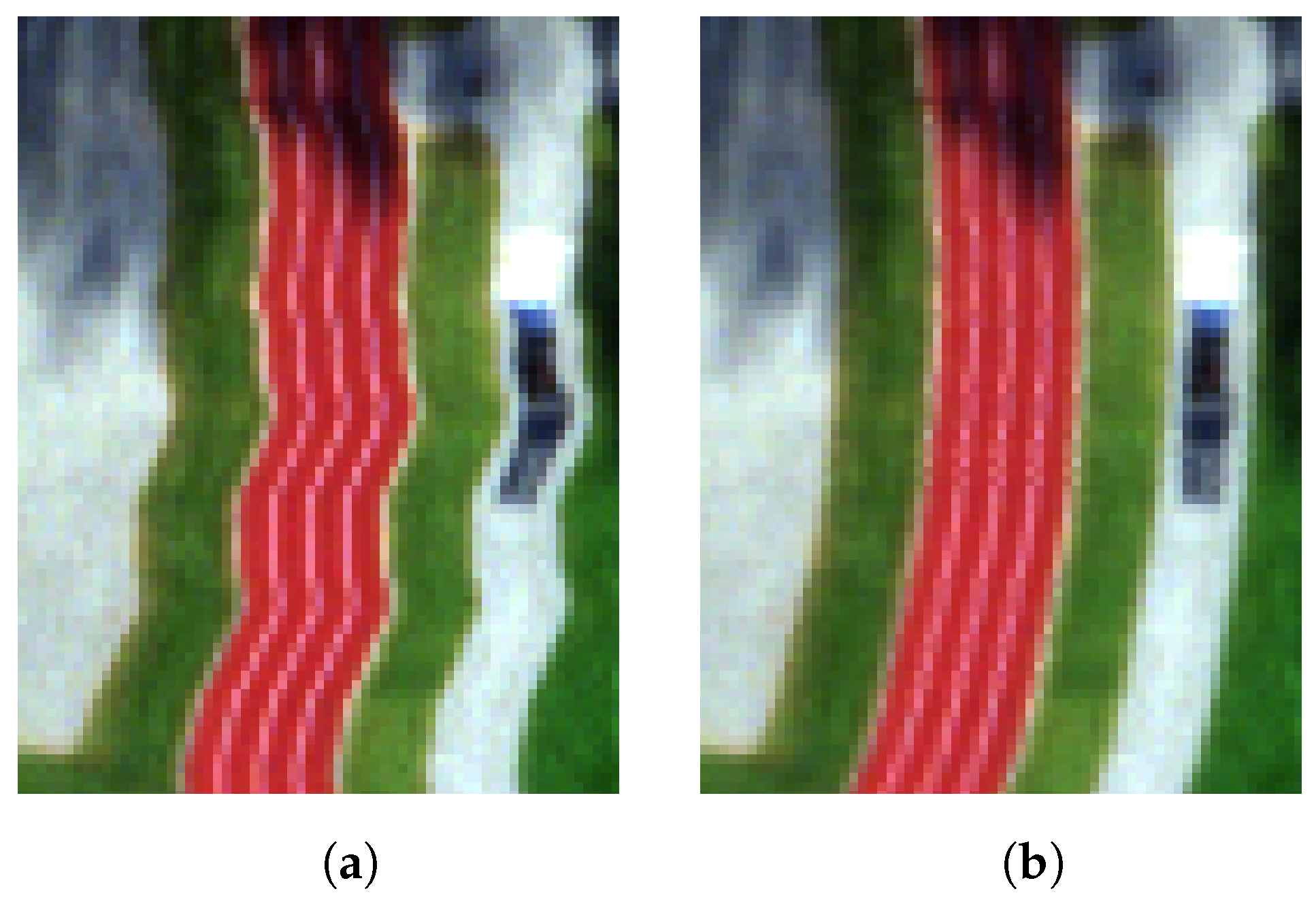
As with the observations used for the bundle adjustment of frame images, the LP image observations are key-point correspondences identified from multiple overlapping images that represent the same tie-point in object space. However, a problem with identifying key points in LP image lines arises, as key-point detectors and descriptors use local 2D image neighborhoods. As LP image lines consist only of a single pixel in one of the image dimensions, a local image neighborhood cannot directly be used to describe the key point in 2D. Thus, several consecutive LP image lines are stacked to form 2D LP image scenes. However, these LP image scenes are subject to significant image distortions, due to the relative camera rotation within an LP image scene (
Figure 4a). Thus, a rotation compensation for this effect is conducted as presented in [
14] (
Figure 4b). The method effectively compensates for the rotations captured using the IMU for a small range of consecutive LP image lines to limit the image distortions in that neighborhood. After observation retrieval, the rotation compensation is no longer considered nor required. The bundle adjustment of LP image lines has shown sub-pixel planimetric accuracy without the use of other data sources [
14].
Each LP image scene is relatively rotation-compensated using the preprocessed trajectory orientations (
Figure 4). Furthermore, BRISK is used to detect and describe the key points within the rotation-compensated LP image scenes, and RANSAC is used for filtering, just as with the frame images. After RANSAC filtering, the observations are registered to the center of the pixel in their respective LP image lines. This center registration of observations makes the observations exact per respective LP image exposure; that is, the observations are independent of small errors in the local image scene neighborhood stemming from the approximate rotation compensation. The LP image observation precision is well-defined from the standard uniform distribution.
3.2. Initialization
The 3D tie-point positions in object space are estimated during the initialization step. The initial tie-point position is computed through finding the closest point of the intersection between the corresponding image rays from multiple images. Corrections to these positions are later estimated in the adjustment.
The second part of the initialization step is the trajectory segmentation. This segmentation is based on the assumption that high-frequency trajectory errors are captured using the INS, while only low-frequency trajectory errors remain after the initial GNSS/INS processing. The background for the trajectory correction model is described in [
13]. To summarize, the trajectory corrections are estimated in the following adjustment only at certain time steps with constant intervals. The corrections at the time of the discrete observations are interpolated using a cubic spline when estimating the parameters in the iterative least squares estimation process.
3.3. Voxel Generation
Voxels are created from the iteratively corrected LiDAR point cloud to effectively include the LiDAR data in the adjustment. The voxel-based method has been shown to ensure the scalability independent of the LiDAR point-cloud density, the efficiency in terms of the processing time, and state-of-the-art accuracy [
13]. No LiDAR points are stored in the voxels themselves, as only certain key properties are needed for each voxel. These metadata are the mean and covariance matrix of the positions, the mean time, and the relative number of intermediate returns of points within the voxel. The voxelization discretizes the LiDAR point cloud into voxels of equal size, such that LiDAR points within the same voxel originate from the same LiDAR scanner and are spatiotemporally close to each other. All points within a voxel stem from the same trajectory segment so that the trajectory corrections associated with a trajectory segment can be estimated from observations formed from the voxels.
The voxels are classified to remove vegetation and to provide meaningful matching between them. Voxels classified as vegetation are removed due to the potential temporal instability and geometric indistinctness in overlapping scans. Classes other than vegetation are used to match voxels of the same class to each other. The voxels are classified into three main groups (
Figure 5):
Planes, based on the eigen transformation of their covariance matrices. Subclasses within the group are horizontal, vertical, and other inclined planes.
Vegetation, based on the number of intermediate returns within a voxel.
Unclassified, representing indistinct geometric neighborhoods not classified as any of the other classes.
All voxels need to consist of some tens of points to provide a sufficient statistical representation of the points within a voxel. Thus, voxels with relatively few points (e.g., <50 points) should be discarded. The method is robust to the exact choice of the voxel size, and finetuning this is not needed [
13].
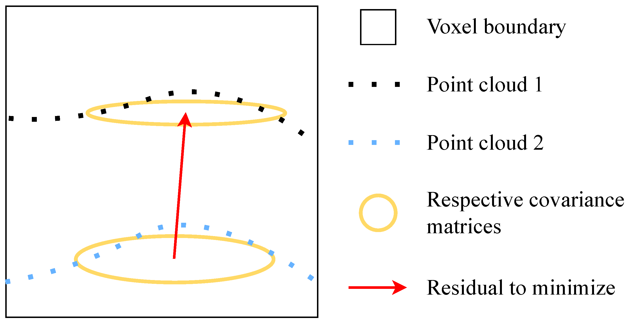
Voxel observations are created from the difference between the mean coordinates of two overlapping voxels. The observation is weighted with the inverse sum of the covariance matrices of the two voxels. These covariance matrices represent the spatial dispersion of points within a voxel. If the voxels represent planar surfaces, only the distance along the normal vector of the surface is minimized.
Hybrid observations are generated between the tie-points from images and the planar voxels from the LiDAR point clouds (
Figure 6). These hybrid observations express the distance between the tie-point position and the mean coordinate of the overlapping voxel classified as a planar surface. The residual is minimized along the normal vector of the plane. The hybrid observation weight is defined by the planarity of the voxel expressed through its eigen-transformed variance. The image rays are, unlike LiDAR pulses, incapable of penetrating certain structures such as vegetation, as images only observe the closest point to the camera. Thus, the voxel means are mostly biased estimates of the tie-point positions. This effectively makes only planar voxels suitable for hybrid observations.
3.4. Parameter Estimation and Correction
Once the observations for the adjustment have been formed between LP image lines, frame images, LiDAR voxels, and tie-points and voxels, these observations are connected to the estimation parameters through the linearization of the respective functional models. The models are referred to as the pinhole camera model, the LiDAR voxel model, and the hybrid voxel–tie-point model, as defined in [
13]. Common for all these models is that they build upon the same trajectory correction modeling, where corrections are estimated only at certain time steps and interpolated using cubic splines.
The trajectory parameters are stochastically constrained using the initial full covariance matrices of the GNSS/INS solution. This helps to control the stability and reliability of the cubic spline trajectory model.
The observation weights are the inverse of the observation covariance matrices for the respective observation types multiplied by the dynamic covariance scaling; see [
29,
30].
3.4.1. Pinhole Camera Model
The image observations to use in the adjustment are the same tie-points in object space identified in multiple images as key-point correspondences. The pinhole model expresses the relationship between a point in the object and image spaces (Equation (
1)) and is expanded to be differentiable with respect to the parameters in a kinematic mapping platform (Equation (
2)). Although the traditional pinhole camera creates a frame image, using the cubic spline model of the trajectory corrections also allows using the pinhole model for LP image lines [
14]. The residual to minimize in the least squares estimation process is known as the reprojection error, i.e., the residual between the measured image coordinates and the image coordinates reprojected from the tie-point in object space (
Figure 7).
represents the coordinates of the point in the camera frame c ( vector). This may be expanded to account for additional image corrections such as lens distortions or the principal point offset.
is the principal distance of the camera in the camera frame (scalar).
is the vector between the camera projection center and the object point in the camera frame.
represents additional image corrections; that is, the nonlinear distortion and the principal point. See [
31].
is the platform position in the map frame m at the time of measurement ( vector).
is the rotation matrix from the platform frame p to the map frame at the time of measurement ( matrix).
is the camera boresight matrix ( matrix), i.e., the rotation matrix from the platform frame to the camera frame.
represents the coordinates of the point in the map frame ( vector).
is the lever arm from the platform origin to the camera optical center expressed in the platform frame ( vector).
Several spatial and temporal factors affect the image observation uncertainty, such as the key-point detection method, uncertainties in the lens distortion and atmospheric refraction models, and motion blur. Thus, the precision estimates of the image observations are infeasible to obtain and are commonly predefined; for example, as a 1/3 pixel.
3.4.2. LiDAR Voxel Model
The LiDAR voxel model expresses the difference between the mean coordinates of two overlapping voxels of the same class (
Figure 8). The model is based on the direct georeferencing equation, which gives the coordinates
of a georeferenced LiDAR point
:
is the lever arm of scanner s in the platform frame ( vector).
is the scanner boresight matrix ( matrix), i.e., the rotation matrix from the platform frame to the scanner frame s.
is the line-of-sight unit vector of the LiDAR point ( vector).
is the range measurement of the LiDAR point (scalar). This may be expanded to account for additional interior scanner parameters, such as the range–scale factor and the range bias.
Since the individual LiDAR points are not stored in the voxels
and
d from Equation (
3) and are instead computed from the scanner-to-voxel geometry based on the mean position of the points within the voxel, the voxel mean time is used to retrieve the time-dependent
and
via the cubic spline interpolation of the trajectory corrections.
The weights of LiDAR voxel observations are the inverse of the sum of their voxel covariance matrices. These covariance matrices describe the spatial dispersion of points within the confined voxel.
3.4.3. Hybrid Voxel–Tie-Point Model
Similar to the LiDAR voxel model, the hybrid voxel–tie-point model is also based on Equation (
3). However, the voxel–tie-point model instead expresses the difference between the mean coordinate of a voxel classified as a planar surface and the tie-point located inside it (
Figure 9). These observations are used to estimate the trajectory, LiDAR scanner, and tie-point corrections.
The weights of the hybrid observations are the inverse of the covariance matrix of the overlapping voxel. However, the relationship between voxels from LiDAR point clouds and tie-points from images is not fully described by the voxel means and covariances. This could for example occur where the LiDAR point sampling is too sparse to capture nonplanar objects where tie-points from images are located. Thus, the hybrid voxel variance has to be inflated.
4. Experimental Results
An experiment was conducted to test the method for multisensor matching from LP images, frame images, and LiDAR point clouds. The experiment was based on a data set acquired from an airplane over the Norwegian University of Life Sciences in Ås, Norway (59.665°N, 10.775°E), in October 2022. The data set originally consisted of 24 flight strips flown at two altitudes as presented in [
14]. However, a reduced experiment with four flight strips was conducted here to imitate a more common operational photogrammetric block, where the flight time should be minimal while still providing enough observations for estimating the sensor and trajectory parameters. The planned data acquisition variables and used sensors are shown in
Table 1. Unlike the experiment in [
14], we introduced both LiDAR data and frame images to the joint adjustment with the LP image lines. All data were captured on the same flight with a dual-hatch airplane, where the LiDAR scanner and frame camera were installed with an INS in the fore hatch. The LP camera was installed in the aft hatch with a separate INS. The flight efficiency was mainly limited by the narrow FoV and minimum operational exposure time of the LP camera. The camera settings are shown in
Table 2. As the used LP HSI camera captures 186 spectral bands, chromatic aberration should be considered. However, this effect is at a sub-pixel level for the HySpex VNIR-1800 camera series used [
14,
32], and thus only a single spectral band at wavelength 592 nm was used in the experiment.
The LiDAR scanner settings of the precisely precalibrated dual-channel system are shown in
Table 3. Common lever-arm corrections (three parameters) and boresight angle corrections (three parameters) were estimated for the two LiDAR channels. Corrections to the boresight angles (three parameters), principal distance (one parameter), radial distortion (three parameters), and tangential distortion (two parameters) were estimated for the frame camera. For the LP camera in the aft hatch, corrections to the boresight angles (three parameters), principal distance (one parameter), radial distortion (two parameters), and tangential distortion (two parameters) were estimated. The constant distance between the two platform pivot points was constrained to a measured constant distance. The trajectory parameters were estimated as corrections to the position (three parameters per time segment) and orientation (three parameters per time segment). Additionally, corrections to each tie-point in object space were estimated. The positional standard deviation (STD) of the processed GNSS/INS solution used as the input for the adjustment was ≤1.3 cm in each horizontal dimension and <2.0 cm in height.
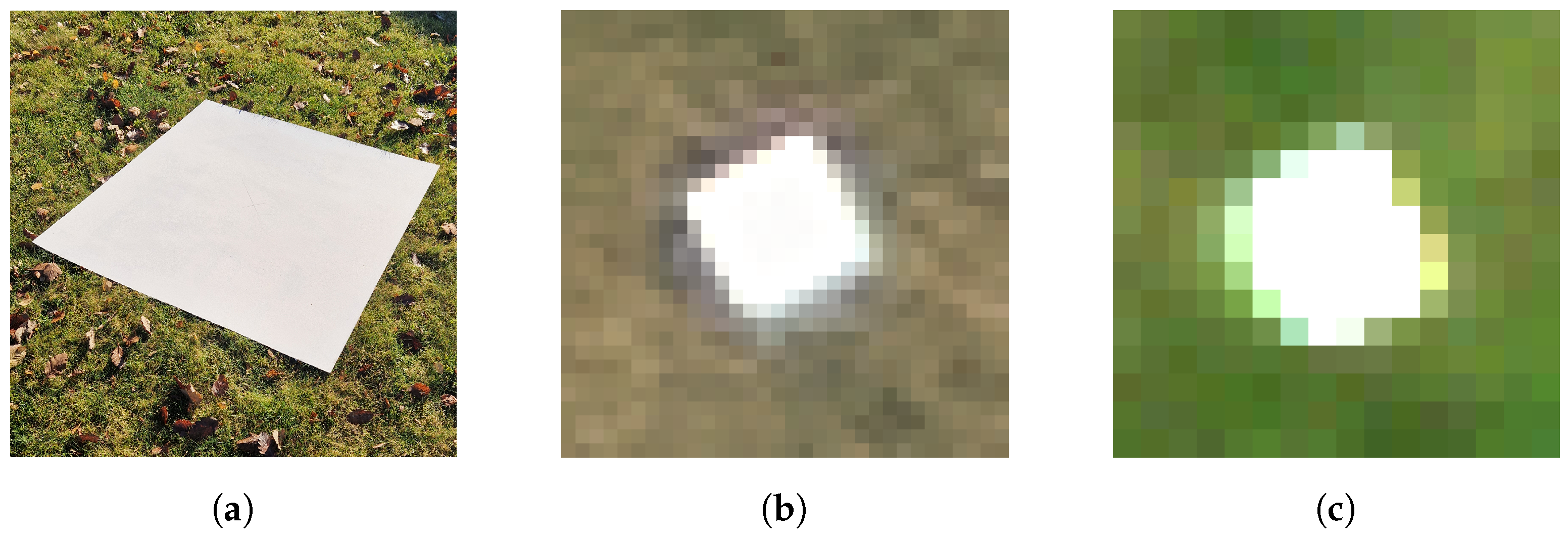
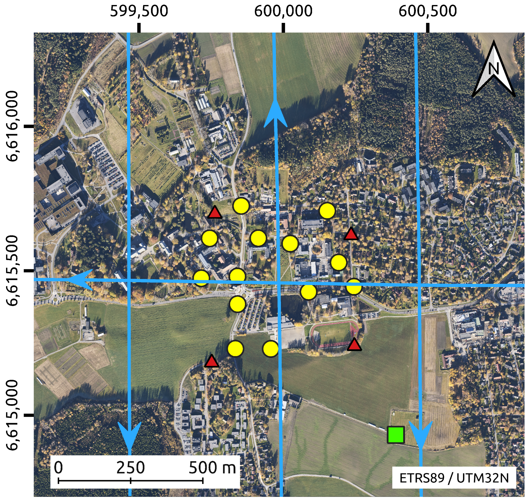
The accuracy after adjustment was assessed using 17 white 1.2 m × 1.2 m reference squares as the groundtruth data. They were placed on the ground within the survey area (
Figure 10). Four of these were used as ground control points (GCPs) for reference and 13 as checkpoints (CPs) for accuracy assessment. This accuracy assessment was conducted by comparing the estimated coordinates of the CP center points to their measured coordinates. The groundtruth centers were precisely measured on the same day as the aerial data acquisition using real-time kinematic (RTK) GNSS positioning on two to three repeated visits. The RTK-based reference data had an estimated precision of approximately 1 cm from the mean position of the repeated visits, which was used as the groundtruth coordinate. All the reference squares had a baseline of <1 km to the nearest permanent GNSS reference station. The locations of the ground reference data are shown together with the flight strips in
Figure 11.
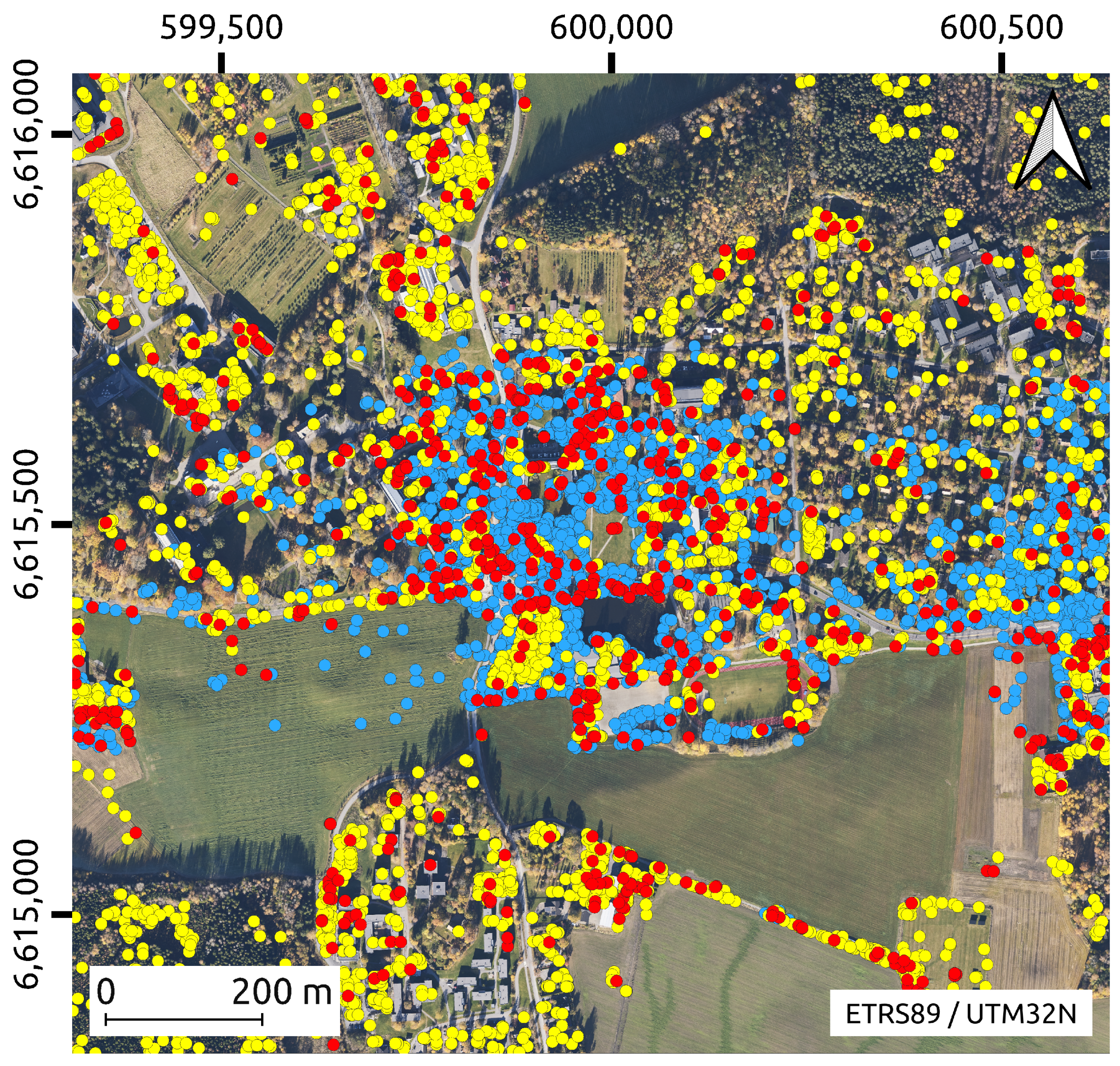
The distribution of the tie-points is shown in
Figure 12. These points were used to form either image observations or hybrid observations to link the LiDAR-derived voxel data to the images. Not shown in the figure are the additional voxel observations formed between overlapping voxels.
The LiDAR voxel size was set to 3 m for both experiments for a sufficient statistical representation of the points in a voxel. The observation weight for LiDAR voxel observations is given by the covariance of the voxel; however, the observation weight from the image observations was set to 1/3 pixel for the frame camera and 1/2 pixel for the LP camera.
Trajectory segmentation time steps of 1, 2, 5, 10, 20, and 30 s were tested to estimate the trajectory corrections (
Figure 13). This time step was evaluated by analyzing the RMSE of the height component of the CP errors for the LiDAR scanner.
Table 4 shows the initial CP error statistics of the LP camera, frame camera, and LiDAR scanner before adjustment. An initial aerotriangulation was performed from the images based on the a priori sensor states to produce these error statistics. The precisely precalibrated LiDAR scanner resulted in cm-accurate point clouds. The median of the STD of the LiDAR points used to compute the initial error statistics was 3.0 cm. This describes the precision of the LiDAR measurements on the CPs.
Table 5 shows the CP error statistics of the LP camera, frame camera, and LiDAR scanner for the experiment with a trajectory segmentation time step of 10 s. Hybrid observations were not formed for these CPs. On the other hand, they were formed for the other tie-points located within a voxel classified as a planar surface. The error statistics are shown as the minimum, maximum, median, interquartile range (IQR), and root mean square error (RMSE). The IQR is approximately 1.35 STDs under the assumption that the data are normally distributed. However, the IQR is robust to outliers. Only the height error is shown for the LiDAR scanner, as the distance along the normal vector of the reference squares was used as the error metric between the groundtruth data and the LiDAR voxels. The median of the STD of the LiDAR points was 1.1 cm.
5. Discussion
The presented method is an extension of earlier work on the hybrid adjustment of images and LiDAR point clouds [
13] and the bundle adjustment of LP HSI [
14]. However, we presented a method showing how to use observations from a LiDAR scanner, frame camera, and LP camera together in a joint hybrid adjustment. This is, to our knowledge, the first published work showing the possible combination of data from these three sensor types to jointly estimate the trajectory and sensor corrections using a common trajectory correction model. Under the assumption that the observations from the different sensors are weighted correctly, the increased number of observations stemming from all these sensors conceptually ensures a better determined system than using the sensor measurements in separate adjustment methods. The limited number of unknown parameters when using the trajectory cubic spline model and the voxelization of the LiDAR point cloud ensures scalability. Additionally, the joint adjustment of data from multiple sensors gives the optimal matching solution for all the used data.
5.1. Experiment Design and Accuracy
In the experiment, the frame camera was installed in the fore hatch in the airplane together with the LiDAR scanner (
Table 1). Thus, observations from these two sensors contribute to estimating the same trajectory parameters using the same modeling of the trajectory corrections. However, the experiment consisted of two platforms that could rotate independently. Thus, the two platforms had separate trajectories with unknown orientation errors. Even though a distance constraint was introduced between the platforms, both trajectories had to be corrected. Thus, only part of the hybrid adjustment potential from data from the three sensor types was fully utilized in the presented experiment. Only the distance was set as a constraint between the platforms, as the angular readings of the gyro mounts are one order of magnitude less accurate than the orientations from the two IMUs. This distance can be measured with mm to cm precision, unlike a constraint on the relative 3D positions between the platforms. The latter would require a transformation through the vehicle body frame and the additional consideration of the gyro-mount precision. Thus, unlike with the constraint on the distance between the platforms, it is neither feasible to use the gyro-mount information to constrain the relative orientation nor the 3D relative position of the two platforms.
The tie-points from the frame camera and those used to generate hybrid observations were evenly distributed in radiometrically inhomogeneous areas in object space (
Figure 12). The LP camera had a very small lateral overlap (
Table 2), which essentially led to tie-points being formed only in the areas where the three parallel flight strips overlapped the crossing flight strip.
The frame camera parameters are well-estimated and provide accurate results for this camera. The LiDAR scanner and frame camera combined provide accurate measurements in all three dimensions, and the platform distance constraint helps to estimate the temporal positional error for the LP camera.
The results show that the planimetric error is of sub-pixel level, whereas the poor base-to-height relation makes the CP height error large when measured from the LP camera. The adjustment of the frame images is very accurate (
Table 5). Thus, the effect of including the hybrid observations between tie-points from the frame images and the LiDAR point cloud is relatively limited, since the photogrammetric block is very strong with significant overlap and a good base-to-height ratio (
Table 2). The experiment was conducted with four GCPs; however, the joint adjustment effectively minimized the residuals between the observations derived from different sensors. Thus, the GCPs are only needed to ensure good absolute accuracy, while the relative consistency between the image and LiDAR data is unaffected by the GCPs. The lifted requirements for dedicated LiDAR ground-control data has been pointed out as a benefit of joint hybrid adjustment in previous studies, e.g., [
3,
33], and is a major advantage compared to processing the data in separate LiDAR strip adjustment and image bundle adjustment per sensor.
There are clear theoretical advantages of combining sensor data from all modalities at the observation level. The current experiment does not allow for an in-depth analysis of the precision and accuracy under different conditions, and serves only to verify the practical application of the suggested approach.
5.2. Observation Retrieval
The observations to be used in the adjustment must be retrieved from the images and the LiDAR point cloud to conduct the joint adjustment. The hybrid observations between the cameras and LiDAR scanner are important to ensure consistent geometric matching between the data from the different sensors.
One main advantage of conducting the joint hybrid adjustment of LiDAR and image data is the ability to estimate temporal trajectory corrections in geometric or radiometric homogeneous areas in object space as long as distinct features exist in one of these domains; the LiDAR scanner will provide valuable observations for the adjustment based on the geometric features, whereas the cameras will provide observations based on the radiometric salinity. For airborne platforms, such as in this experiment, the LiDAR scanning will result in an abundant number of observations, effectively representing the ground level. On the other hand, the cameras will provide observations effectively describing the planimetric discrepancies.
The hybrid observations from airborne platforms, such as in this experiment, often only describe the height errors. This is mainly owing to the limited number of hybrid observations being formed on non-horizontal planes from the aerial data acquisition. As the residual is minimized along the normal vector for planes detected in LiDAR voxels, the observability of parameters explaining the planimetric errors in the LiDAR point cloud is limited. This is also true for the voxel observations used to match LiDAR point clouds from different flight lines to each other. As only very few vertical surfaces are observed from the airborne LiDAR scanner, only the inclined surfaces (e.g., inclined roofs) and indistinct voxels contribute to minimizing the planimetric error. Even though the observations formed from indistinct voxels will contribute to estimating the parameters to minimize the planimetric error, these observations have a relatively low weighting compared to the planar surfaces as expressed by their respective covariance matrices. The exact voxel size has earlier been shown in [
13] to not be critical for the method, as long as it is reasonably chosen to include planar surfaces. The 0.3 cm vertical LiDAR RMSE with a segmentation time step of 10 s shown in
Figure 13 indicates that the ground level was geometrically well-defined from LiDAR measurements. However, vertical structures are difficult to detect from airborne LiDAR scanning, which limits both the observability of parameters connected to the horizontal displacement and the possibility of addressing the horizontal LiDAR point cloud accuracy. All in all, the photogrammetric block ensures sub-pixel planimetric accuracy and the combination of LiDAR and photogrammetric adjustment compensate each other to increase the accuracy in all three dimensions.
It is challenging to accurately form observations between RGB frame images and LP HSI. The LP cameras are often used for HSI, which typically have entirely different camera properties than standard RGB frame cameras (e.g., spectral bandwidth, spectral response, and chromatic aberration). Thus, an analysis of the spectral bands in the HSI camera to imitate the spectral signal as recorded by the RGB camera would be necessary if salient key points in two images from the two different camera types were to be confidently matched. Alternatively, the approach proposed in the experiment is robust to the different camera types (i.e., HSI and RGB cameras), as the image observations are retrieved separately in different preprocessing steps for the two cameras (
Figure 3).
Some hybrid observations are outliers, just as with any other observation material from real-world data. Tie-points from images are located in image neighborhoods with distinct radiometry, which are often found on geometrically sharp structures relative to the surrounding planar surface. An example of this from the presented experiment is shown in
Figure 14. The LiDAR point cloud is not always dense enough, nor is the footprint small enough, to precisely measure and express such distinct geometric structures through the voxel covariance matrix. Thus, the hybrid observation variance should in these cases be inflated to prevent over-optimistic observation weighting.
Hybrid observations between the tie-points and LiDAR voxels help to estimate the image depth, where the observations of the tie-points are found in the image. However, the accurate estimation of parameters describing the image depth, mostly the principal distance, still depends on the view geometry between the image rays observing a tie-point in object space. Furthermore, for an airborne platform, the limited LiDAR view angle limits the ability to correct horizontal errors with LiDAR scanners. Consequentially, very few tie-points located on vertical structures are used to form hybrid observations. As the tie-point positions in object space are initially estimated from the image observations (
Figure 3), they need to be observed in at least two images of cameras with similar radiometric properties. This further limits the number of hybrid observations, as some distinct radiometric image measurements may be visible in only a single image. However, the alternative ray-casting on the LiDAR point cloud required for computing the initial tie-point coordinates is a computationally expensive operation.
5.3. Trajectory Segmentation
The trajectory errors are known to change to such a degree that they degrade the resulting LiDAR scans for a flight strip, e.g., [
22]. Hence, a higher-order trajectory correction model is appropriate. For cameras, several images are often taken per second; thus, the trajectory parameterization per image exposure is often an over-parameterization. Additionally, it is common for several cameras to be installed on the same platform (e.g., in oblique imaging). In such cases, the method proposed here takes advantage of all the observations from all the used sensors to estimate the same trajectory corrections.
Figure 13 shows that the choice of the trajectory segmentation time step is not critical to achieving accurate results. However, the shorter trajectory segmentation time steps generally offer higher accuracy with increased model complexity.
Normally, the number of retrieved observations is extremely high compared to the required parameters when using a trajectory segmentation time step of some seconds; thus, the method is robust to the choice of this time step. Using a similar approach, a trajectory segmentation time step of ≤10 s has been shown to provide accurate results for UAVs; see [
22].
Certain sensor parameters, such as the boresight correction angles of the LP camera, are challenging to estimate correctly without a rigorous trajectory error model that considers the temporal changes in trajectory errors. When using a trajectory time segmentation as presented, any arbitrary sensor used for kinematic mapping can strengthen the trajectory error estimation as long as the functional model is known, the observations are reliable, and precise time stamps are provided for the data.
7. Conclusions
A novel theoretical development was presented, and an experiment was conducted to show that a scalable joint hybrid adjustment of data from LiDAR scanners, frame cameras, and LP cameras is achievable. To the authors’ knowledge, this is the first time the joint matching from observations from these three modalities has been demonstrated. In such an adjustment, the observations from the three sensors contribute to estimating the same corrections to the trajectory and sensor interior orientations. This allows for the use of observations from the different sensors directly in the joint adjustment, rather than adjusting the data in a subsequent process. Tie-points can be constrained to lie on planar surfaces from the LiDAR data, thus leading to increased height accuracy. The planimetric accuracies were 1/7 RMSE of the ground sampling distance (GSD) for the frame images and 1/2 RMSE of the GSD for the LP images in each of the two planimetric dimensions. In addition to the sensors used here, the general trajectory error formulation allows for observations from any arbitrary sensor with a known functional model, reliable observations, and precise time stamps to be included in the joint adjustment of the data from kinematic mapping platforms.
