1. Introduction
Remote sensing technology is a powerful tool for acquiring geographic environmental information and land resource data [
1]. Optical remote sensing satellites offer detailed Earth observations, making them significant for monitoring land, forests, and the atmosphere [
2]. However, cloud and snow cover can often obscure the Earth’s surface, hindering the observation of geomorphic features and surface characteristics [
3]. Additionally, understanding climate change, investigating hydrological resources [
4], and issuing snow disaster warnings all depend on accurate segmentation of clouds, snow, and lakes in remote sensing imagery [
5].
The similar reflectivity characteristics of clouds and snow in visible and near-infrared bands present challenges for distinguishing between them [
6], while lakes and cloud shadows exhibit similar low reflectance in visible bands, further complicating segmentation. Various algorithms have been proposed to address this issue, resulting in three primary technical approaches: spectral threshold-based methods [
7], classical machine learning-based methods [
8], and deep learning-based methods [
9]. Spectral threshold methods are straightforward, and they rely heavily on prior knowledge and struggle in complex scenes [
10]. Classical machine learning methods require manual selection of image features for classification [
11], achieving high accuracy but demanding significant manual effort [
12]. Deep learning, on the other hand, automatically extracts features and achieves high-precision segmentation, but it is heavily reliant on dataset quantity and quality, often requiring labor-intensive manual annotation [
13].
Recent advancements in deep learning have significantly improved cloud, snow, and lake detection in remote sensing data [
14]. Deep neural networks can automatically capture texture, shape, and contextual information, often outperforming traditional methods [
15]. Previous studies have successfully applied deep neural networks to detect these features. Guo et al. [
16] suggested a neural network with a codec structure to extract cloud regions in remote sensing images. Qu et al. [
17] proposed a parallel asymmetric network with dual attention, which has both a high detection accuracy and a rapid detection speed for detecting clouds in remote sensing images, but it has no advantage in the case of the coexistence of cloud and snow. Chen et al. [
18] used a Convolutional Neural Network (CNN) to segment the water bodies of lakes and demonstrated that deep learning methods were more accurate than traditional methods. However, this method cannot perceive global contextual information, so the segmentation results have a low degree of continuity. To improve the perception of global information to achieve dense prediction of lake pixels, Hu et al. [
19] designed a multibranch aggregation module using dilated convolutions to improve the prediction accuracy of lakes.
Current research often concentrates on a singular neural network model, leading to notable disparities across studies due to varying sample settings and parameters. Moreover, coarse spatial resolution and significant differences in object size contribute to considerable errors in object recognition outcomes. The successful deployment of the Sentinel-2 satellite has opened new avenues for object identification and detection. Sentinel-2, equipped with a high-resolution multi-spectral imager (MSI), facilitates land monitoring by providing comprehensive imagery of vegetation, soil and water cover, inland waterways, coastal regions, and more [
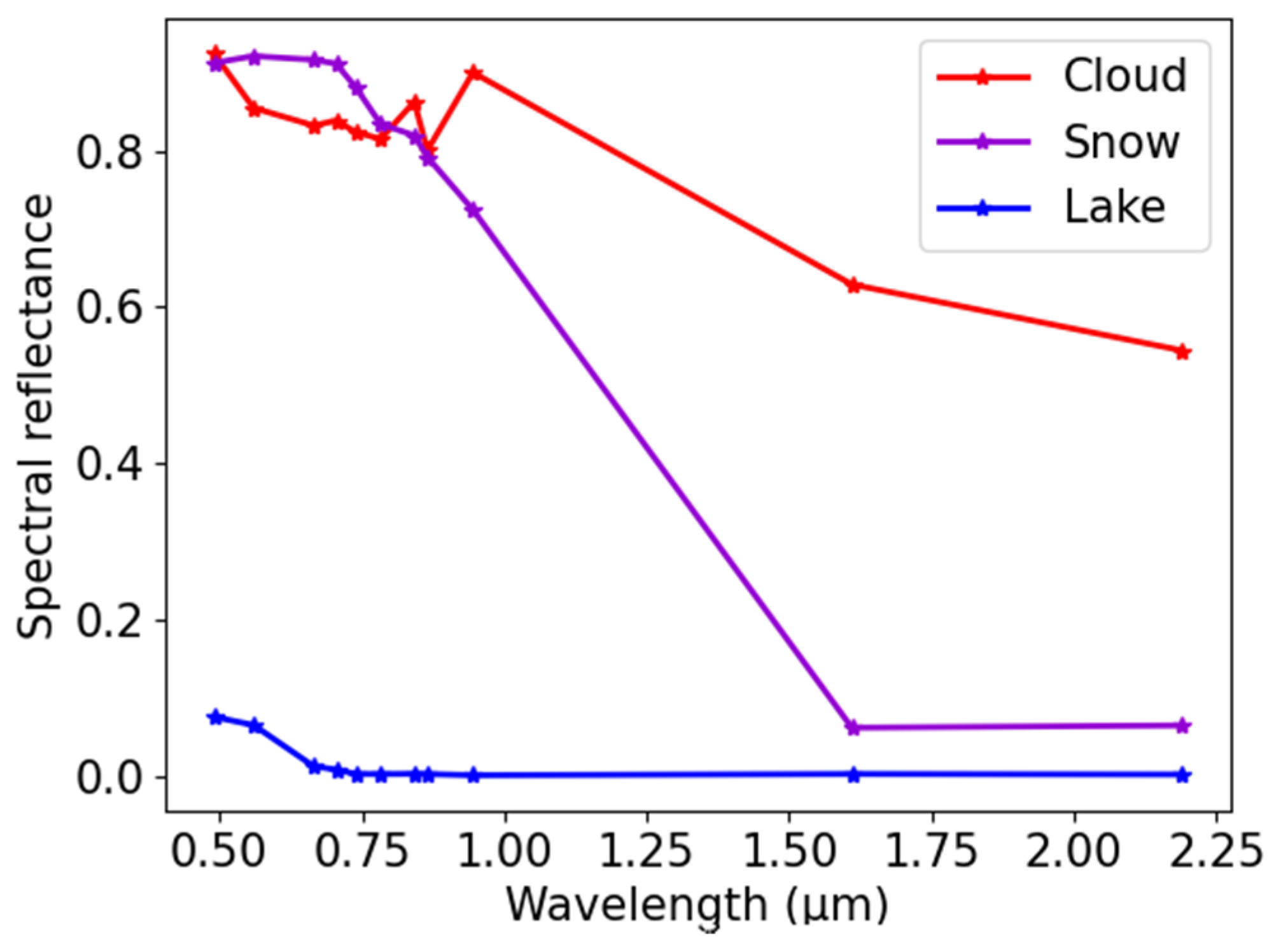
20]. Snow exhibits high reflectance in the visible light spectrum and low reflectance in the short-wave infrared spectrum, while clouds demonstrate higher short-wave infrared reflectance compared to snow. Lakes, conversely, exhibit low reflectance in the visible light band.
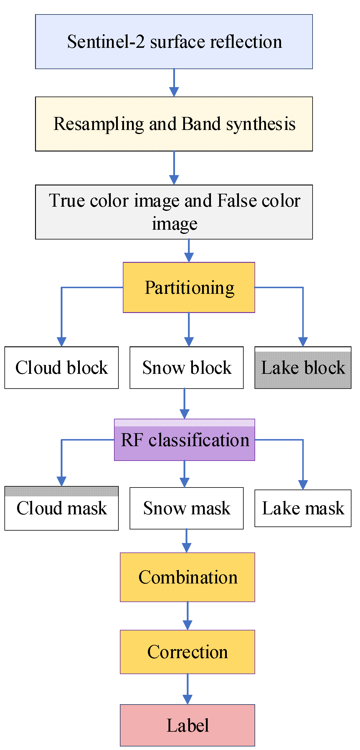
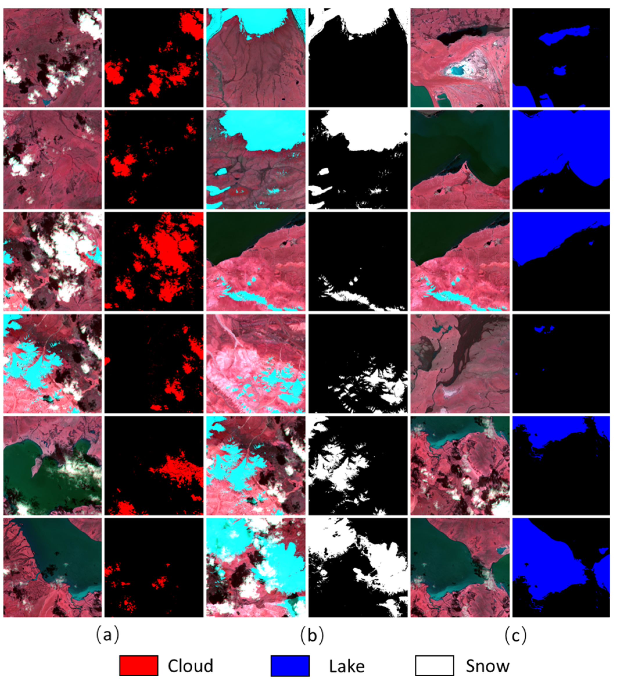
In this study, we investigate the factors influencing the performance of neural network algorithms for detecting clouds, snow, and lakes using Sentinel-2 remote sensing images. We propose a two-stage random forest algorithm for constructing a labeled dataset and then analyze the influencing factors of semantic segmentation networks from six perspectives: model architecture, encoder, learning rate adjustment strategy, loss function, input image size, and input bands.
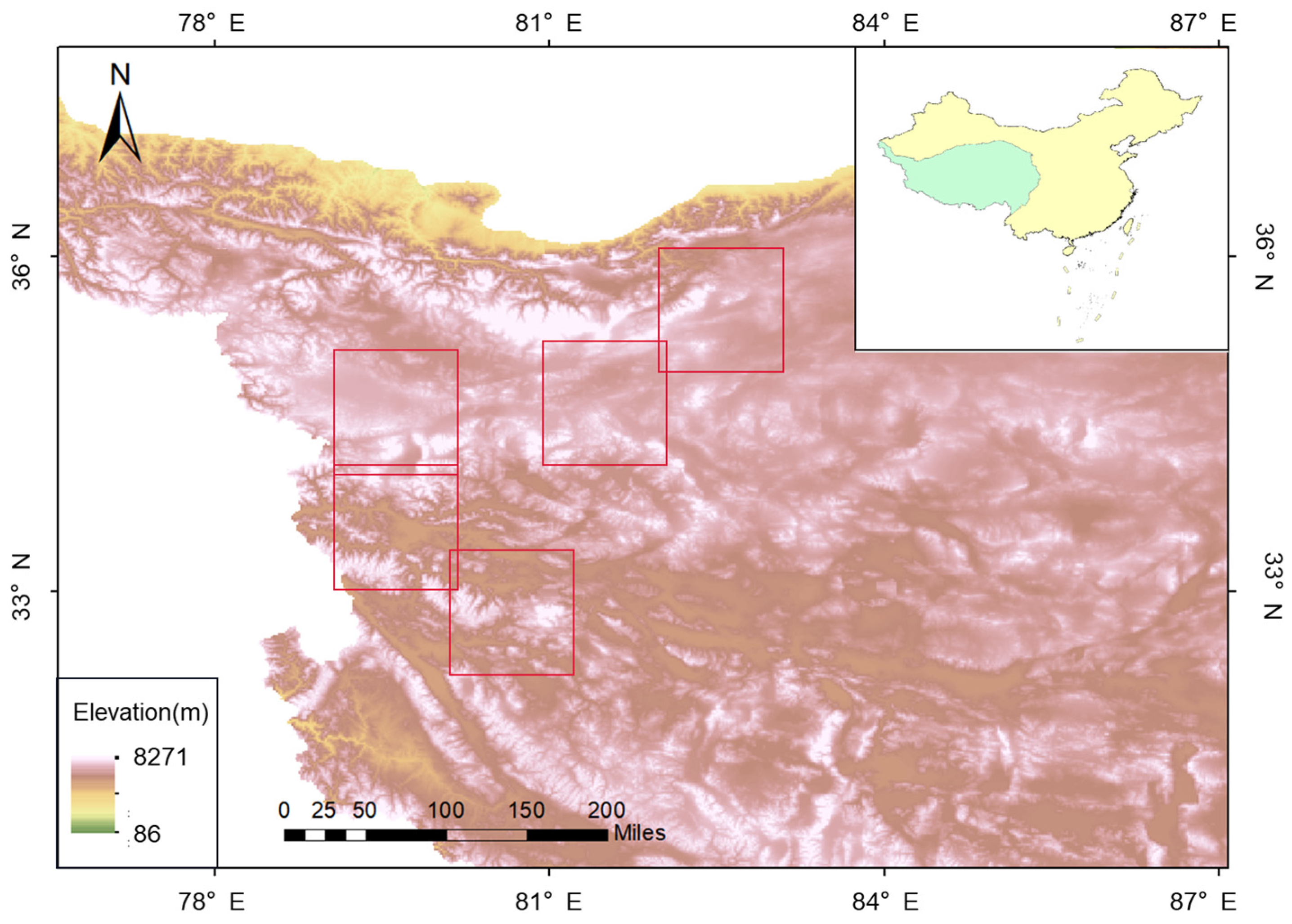
Section 2 introduces the research area and data.
Section 3 introduces the six influencing factors of the neural network model.
Section 4 details the experimental setup and parameter selection.
Section 5 presents the results and analysis.
Section 6 discusses the results of the work.
Section 7 concludes this work.
3. Factors Affecting the Performance of Neural Network Algorithm
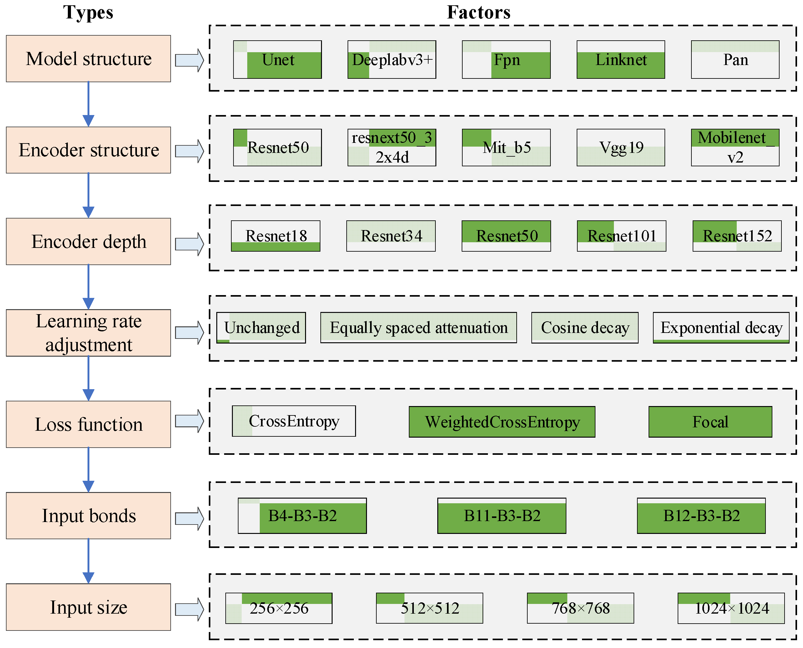
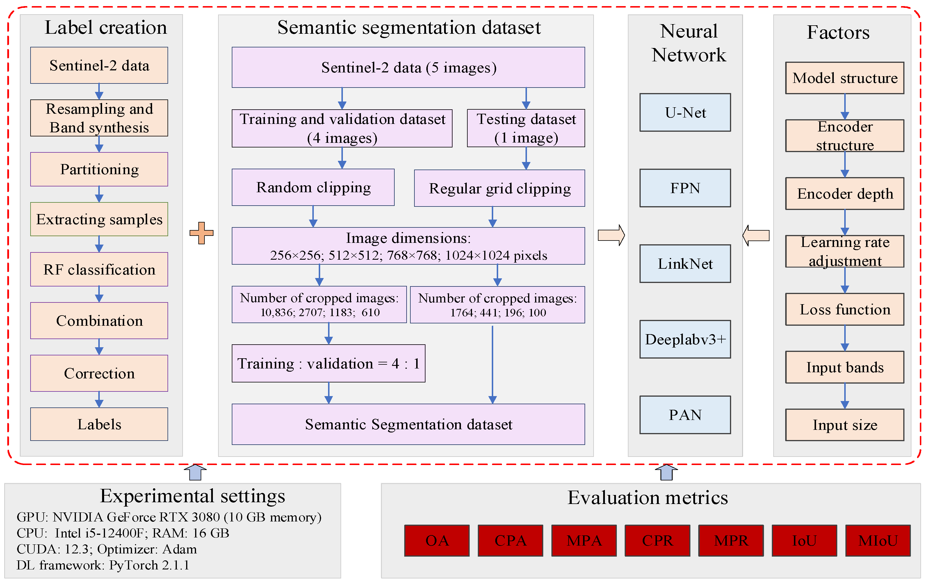
Utilizing the semantic segmentation dataset encompassing clouds, snow, and lakes, this study delves into the influence of six pivotal factors on model performance: model architecture, encoder, learning rate adjustment strategy, loss function, input image size, and input bands (
Figure 7). Each factor underwent systematic exploration, with parameters demonstrating optimal performance in the preceding step serving as the benchmarks for subsequent adjustments. We did not explore all possible parameter combinations, as this would be excessively labor-intensive and likely have minimal impact on the results. Additionally, we did not strictly distinguish between glacier and snow; in this study, the term ‘snow’ refers to both snow and glacier.
3.1. Model Architecture
The application of neural networks in semantic segmentation relies heavily on effective model construction and architecture optimization. In this study, the impact of different model architectures on final performance was evaluated, encompassing U-Net [
23], Deeplabv3+ [
24], Feature Pyramid Network (FPN) [
25], LinkNet [
26], and Pyramid Attention Network (PAN) [
27] (
Table 3). U-Net, renowned for its efficacy, integrates encoder and decoder feature layers via skip connections and facilitates the fusion of features from diverse receptive fields. This characteristic enables the retention of both low-level shallow features and high-level semantic features, rendering it particularly suitable for datasets with limited sample sizes. FPN employs a feature pyramid to amalgamate information from various scales, adeptly managing objects of varying sizes and categories. By leveraging this pyramid structure, FPN effectively handles multi-scale features, enhancing segmentation accuracy. DeepLabv3+ adopts an encoder-decoder architecture, with the encoder incorporating dilated convolutions to augment the receptive field without compromising information integrity. Furthermore, a spatial pyramid pooling module with dilated convolutions at the encoder’s end facilitates the fusion of multi-scale information, contributing to comprehensive feature representation. LinkNet, inspired by U-Net’s architecture, introduces modifications to the connection mechanism between the encoder and decoder. By directly transmitting input and output from the encoder to the decoder, LinkNet minimizes information loss, thereby enhancing segmentation performance. PAN employs a unique approach to feature aggregation, consolidating feature maps from different levels to ensure maximal utilization of information within each map. By mitigating information loss during cascading and preserving detailed information, PAN exhibits promising potential for semantic segmentation tasks. Each model architecture offers distinct advantages, tailored to specific segmentation requirements and dataset characteristics. By systematically evaluating these architectures, researchers can discern the most suitable model for a given task, thereby optimizing segmentation performance.
3.2. Encoder
The encoder-decoder architecture plays a pivotal role in semantic segmentation tasks, serving as the backbone for feature extraction and subsequent pixel-level classification. Understanding the characteristics and trade-offs of different encoders and depths is crucial for designing efficient and effective segmentation networks tailored to specific tasks and computational resources. We will analyze the influence of different encoder structures and depths on neural network performance in this work.
The encoder is responsible for extracting hierarchical feature representations from input images. In the context of semantic segmentation, it compresses the original image while retaining crucial semantic information. Contextual understanding, facilitated by an effective receptive field, is vital for accurate segmentation. Five commonly used encoders—Vgg19 [
28], ResNet50 [
29], ResNext50_32x4d [
30], MobileNet_v2 [
31], and Mit_b5 [
32]—are selected to discuss the influence of encoder structure on neural network performance in this study.
Vgg19 comprises five convolutional layers separated by max-pooling operations. Each convolutional layer consists of multiple convolution and ReLU operations. Vgg19 is relatively simple compared to other architectures and captures meaningful feature representations. ResNet50 introduces residual connections to address the vanishing gradient problem in deep networks. By allowing information to flow directly across layers, ResNet enhances convergence speed and accuracy, making it a popular choice for various computer vision tasks, including semantic segmentation. Building upon ResNet, ResNext50_32x4d incorporates group convolution to reduce the number of hyperparameters while maintaining accuracy. This architecture enhances parameter efficiency, making the model more suitable for running equipment with small video memory. MobileNet_v2 employs separable convolution, which decomposes the convolution operation into depthwise and pointwise convolutions. This reduces the number of parameters and computational complexity, making MobileNet_v2 particularly efficient for mobile and embedded applications. Mit_b5 merges the self-attention mechanism of the Transformer model [
33] with the feature extraction capability of CNNs. By leveraging both global context information and local features, Mit_b5 enhances the accuracy and efficiency of semantic segmentation, especially in capturing long-range dependencies.
Encoder depth refers to the number of layers used for feature extraction. Deeper encoders can learn more complex features, allowing the network to capture intricate patterns and structures in the data. However, increasing depth also amplifies the number of parameters and computational complexity, potentially leading to longer training times. The ResNet model offers varying depths. ResNet18 (with the number “18” indicating the depth), ResNet34, ResNet50, ResNet101, and ResNet152 were selected to explore the impact of encoder depth on segmentation performance.
3.3. Learning Rate Adjusting Strategy
The strategy for adjusting the learning rate plays a pivotal role in the effective training of neural networks. In the initial stages of training, employing a high learning rate enables the model to rapidly approach an optimal solution. However, an excessively large learning rate can lead to instability in the optimization process, thereby impeding the acquisition of an optimal solution. Gradually decreasing the learning rate facilitates more effective convergence toward either a global or local optimum while simultaneously reducing the risk of model overfitting.
In this study, we deployed four prevalent learning rate adjustment strategies to examine their influence on training outcomes. Let e denote the number of epochs completed during training, and
represent the learning rate until epoch e. We initialize the learning rate at 0.001. The strategies and their corresponding learning rate curves are delineated below (
Figure 8):
(1) Remaining constant: The learning rate remains unchanged throughout the training process. The curve is a straight line, as the learning rate does not change.
(2) Equally spaced decay: The learning rate decreases at equally spaced intervals.
The learning rate decreases from 0.001 to 0.0001 linearly.
(3) Cosine decay: The learning rate follows a cosine function to decay smoothly over time.
The learning rate follows a cosine function with a period of 20 epochs, decreasing and then increasing within each period.
(4) Exponential decay: The learning rate decays exponentially, reducing more rapidly in the initial stages.
The learning rate decreases smoothly throughout the training.
3.4. Loss Function
The loss function plays a pivotal role within neural networks, serving to quantify the disparity between the model’s predicted output and the actual label. Throughout the training process, minimizing the loss function becomes imperative to align the model’s predictions closely with the true labels. The selection of an appropriate loss function significantly influences the efficacy of training and the performance of the model. Cross-Entropy (CE) [
34] loss function stands out as a widely employed choice for semantic segmentation tasks. Its definition is outlined as follows:
where
N represents the number of pixels;
M represents the number of classes;
y is an indicator function that is 1 if the true class of sample
i is
c, and 0 otherwise;
p represents the predicted probability that the observed sample
i belongs to class
c.
In the Tibetan plateau, where mountains dominate the majority of the area, there is a pronounced data imbalance in the sample distribution. Specifically, one or more classes are significantly underrepresented compared to others. This imbalance poses a challenge as it biases the loss function, leading to poor performance of the model, particularly on smaller samples such as clouds and lakes. To mitigate this challenge, the Weighted Cross Entropy (WCE) loss function was introduced in this study. This loss function incorporates weighting factors into the Cross Entropy (CE) loss function, thereby rectifying the distribution of the loss function. The formulation of WCE is delineated as follows:
where
wc is the weight assigned to class
c. By assigning higher weights to underrepresented classes, WCE ensures that the model pays more attention to these classes during training, improving its performance on small samples. This weighted approach helps mitigate the dominance of the majority classes and enhances the overall accuracy of the semantic segmentation model.
Moreover, FocalLoss [
35] offers a solution by incorporating a focus factor that diminishes the loss impact of well-classified examples, thereby directing more attention toward challenging-to-classify samples. This is accomplished by assigning a weighting factor that tends toward 0 for accurately classified samples and 1 for misclassified ones. Consequently, the loss value attributed to accurately classified samples decreases, while that of misclassified ones remains relatively unchanged. This approach effectively amplifies the influence of inaccurately classified samples within the loss function. The formulation of Focal Loss is presented as follows:
where γ is a focusing parameter that adjusts the rate at which easy examples are down-weighted, and
is the weight assigned to class
c.
In this study, CE was employed as the benchmark to assess the efficacy of WCE and Focal Loss in tackling the data imbalance prevalent in cloud, snow, and lake segmentation. Through a comparative analysis of these loss functions, the objective is to investigate the potential of WCE and Focal Loss in alleviating the evaluation errors posed by imbalanced datasets and enhancing model performance.
3.5. Different Input Image Size
The size of the input image significantly impacts the performance of the model. A larger input size equips the model with more detailed information, thereby enhancing its ability to generalize and capture finer details and features within the data. Consequently, this often results in more precise and resilient predictions. However, larger input image size also increases computational complexity and processing time. Conversely, if the input image size is too small, critical information may be lost, potentially leading to model overfitting and undermining the neural network’s accuracy and generalization capacity. Hence, selecting an appropriate input image size tailored to specific application scenarios is very important for achieving optimal performance while striking a balance between accuracy and computational efficiency. In this study, five remote sensing images are cropped into sizes of 256 × 256, 512 × 512, 768 × 768, and 1024 × 1024 to serve as inputs for the neural network.
3.6. Different Band Combinations
Satellite remote sensing images capture both the reflected electromagnetic wave information and the thermal radiation emitted by ground objects. Due to various structural, compositional, and physical-chemical properties, the reflection and thermal radiation patterns of different ground objects are distinct. For instance, water bodies typically exhibit low reflectivity within the wavelength range covered by most remote sensing sensors due to their efficient absorption of solar energy. Conversely, snow demonstrates high reflectivity in visible light (VIS) and low reflectivity in short-wave infrared (SWIR), facilitating its effective differentiation from clouds.
Sentinel-2 incorporates three SWIR bands (
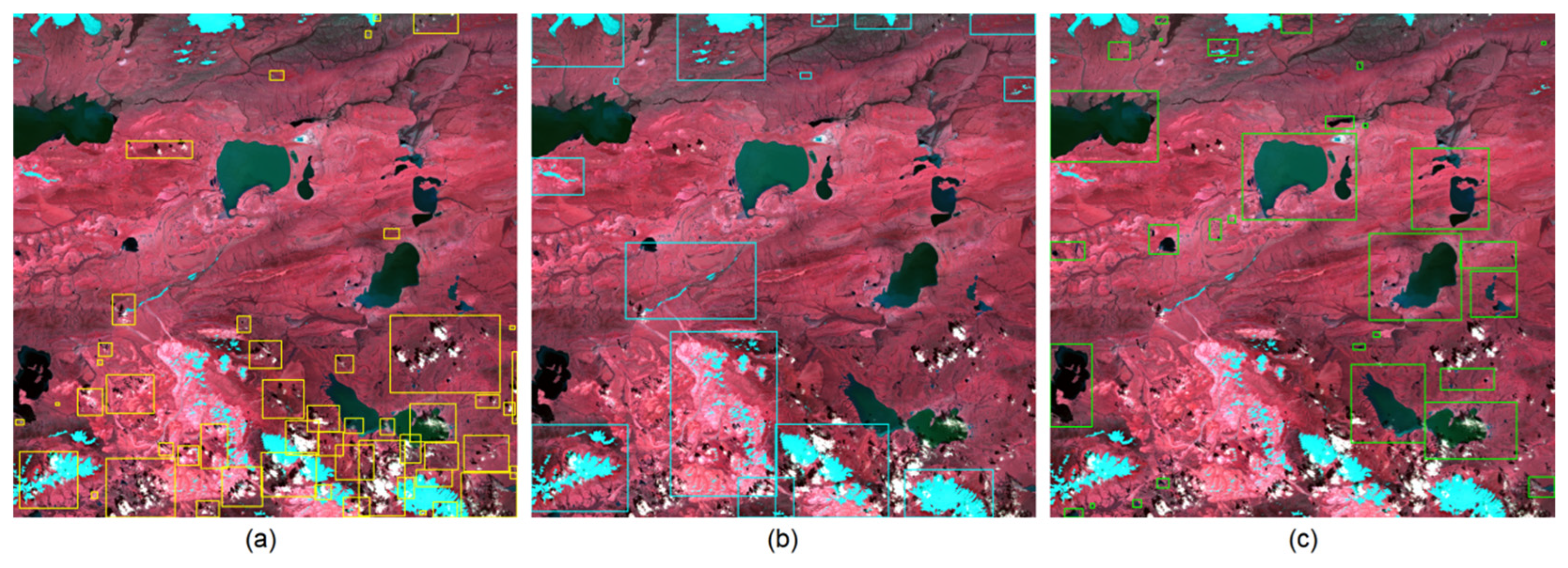
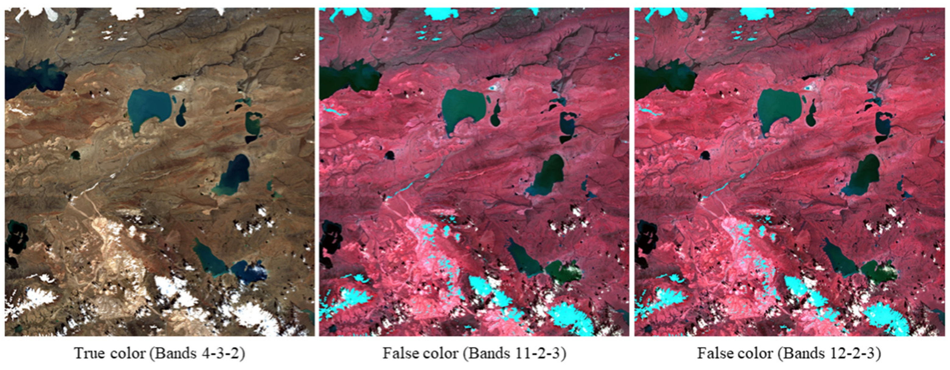
Table 1): Band 10 (1.375 um), Band 11 (1.610 um), and Band 12 (2.190 um). Band 10 (referred to as B10 hereinafter, similarly for other bands) is designed for cirrus detection and records Top-of-the-Atmosphere (TOA) reflectance rather than surface reflectance, which is omitted from L2A level data. Consequently, this investigation concentrates on bands B11 and B12. These bands are combined with visible bands B2 and B3 to produce true-color or false-color images. Specifically, combinations such as bands 4-3-2, 12-2-3, and 11-2-3 are used to explore the impact of different band combinations on the segmentation of clouds, snow, and lakes (
Figure 9).
5. Result and Analysis
5.1. Deep Learning Models Structure
Table 5 presents the evaluation metrics for U-Net, Deeplabv3+, FPN, LinkNet, and PAN models on the semantic segmentation dataset of clouds, snow, and lakes. It is evident that all models achieve high OA, exceeding 96%. However, the MPA is notably lower than the OA, with a maximum difference of up to 15% between the MPA and OA for the LinkNet model. This discrepancy is mostly due to the imbalance in the data categories, i.e., the background category comprises a significantly larger number of pixels compared to the target categories. Consequently, even if the segmentation accuracy for the target categories is very low, the overall accuracy remains high, indicating that OA is not a reliable metric for evaluating performance on imbalanced datasets. Additionally, the MPR for all models is above 95%, suggesting that there are a few missed points across categories. However, the large difference between MPR and MPA highlights the issue of data imbalance. That is, categories with a larger number of instances are often correctly identified, whereas those with fewer instances are less accurately segmented. Among all the models, LinkNet exhibited the lowest MIoU at 79.61%, while FPN achieved the highest MIoU at 85.69%, demonstrating the best performance.
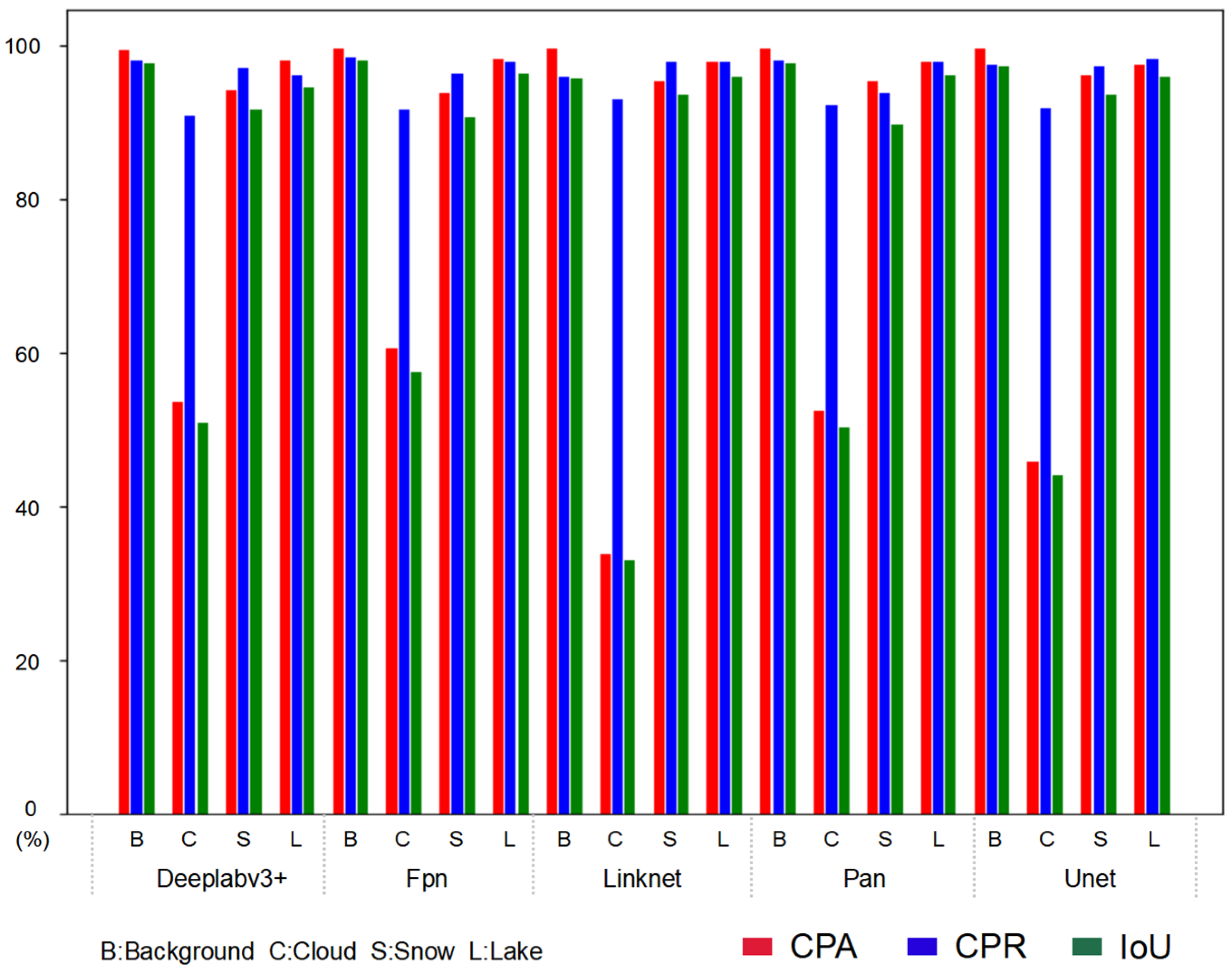
Figure 11 presents the CPA, CPR, and IoU metrics from five models to detect clouds, snow, and lakes. The various metrics of snow and lake are almost above 90%, which means that the segmentation accuracy of these two categories is very high. However, the IoU of most models for cloud segmentation is almost below 60%. Linknet’s cloud segmentation IoU was the lowest at only 30%, significantly reducing the value of MIoU. In contrast, FPN’s cloud segmentation IoU was the highest, at 60%. The reason for poor performance for cloud segmentation for all models is that a large number of pixels from other categories are misclassified as clouds.
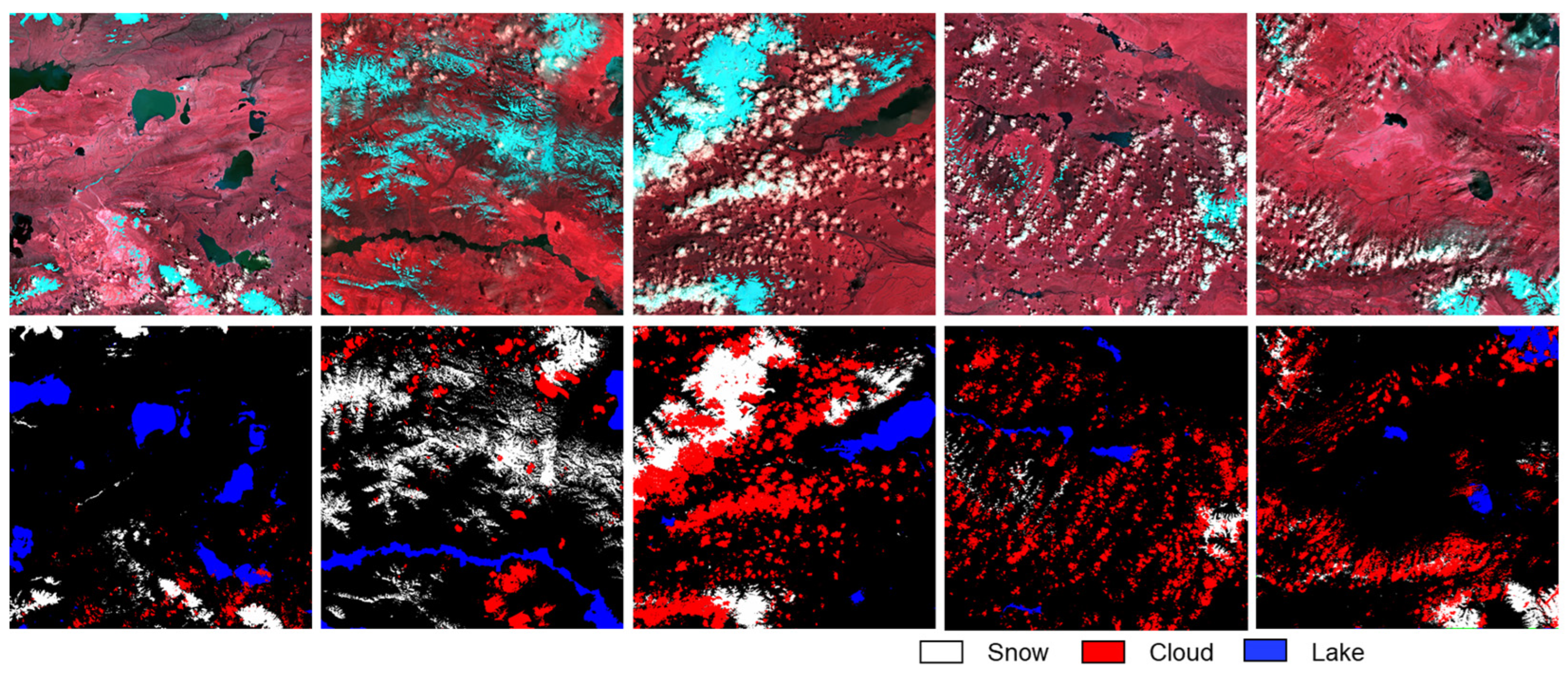
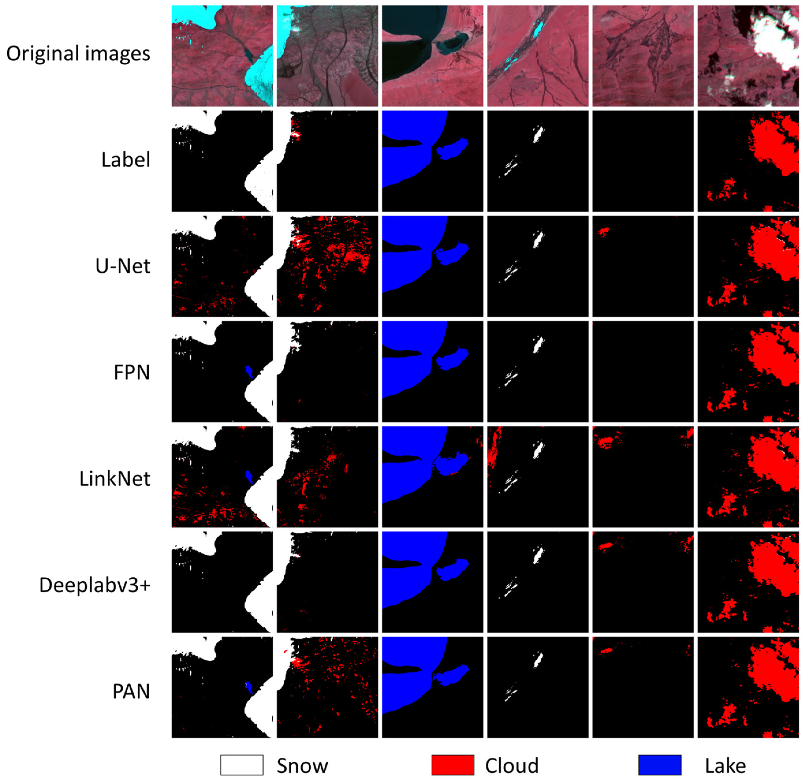
The prediction outcomes of each model are depicted in
Figure 12. Notably, LinkNet exhibits a pronounced misclassification of clouds, with a substantial number of background pixels erroneously categorized as clouds. This misclassification directly undermines LinkNet’s cloud segmentation accuracy (low IoU). Structurally, LinkNet diminishes subsampling operations in the encoder to retain spatial information, yet this also preserves excessive noise during training, leading to significant disruptions in cloud recognition. In contrast, FPN demonstrates superior segmentation performance compared to U-Net, Deeplabv3+, PAN, and LinkNet, owing to its simpler structure and effective utilization of a pyramid structure to merge shallow (small size of receptive field) and deep (large size of receptive field) features. Simple target objects, such as clouds, snow, and lakes, can be effectively detected using spectral and texture features without relying solely on complex semantic features. Consequently, opting for a lightweight network like FPN may yield superior results. The large size variations within the ground objects require a network capable of producing outputs with varying receptive field sizes; thereby, the feature pyramid structure is particularly suited for segmenting clouds, snow, and lakes.
5.2. Encoder Type and Depth
Based on the above conclusions, FPN is identified as the best network structure among the selected models. Therefore, the following section will discuss the influence of the encoder on the performance of the FPN model.
- (1)
Encoder structure analysis
We selected five encoders, i.e., Vgg19, Resnet50, Resnext50, MobileNet_v2, and Mit_b5, to analyze their impact on model performance (
Table 6). Resnet50, Resnext50_32x4d, and MobileNet_v2, which employ residual structure, exhibited approximately 20% higher MIoU than Vgg19, which does not use a residual structure. This underscores the effectiveness of residual connections. From the perspective of parameter count, MobileNet_v2 significantly reduces the number of parameters (only 4.22 million (M) parameters) and the computation load due to its deep separable convolution structure. This makes it more suitable for datasets with a small amount of data and relatively simple segmentation tasks. In contrast, Mit_b5 has a substantial number of parameters (83.33 M) due to its extensive use of multi-head self-attention mechanisms. This large parameter count needs a considerable amount of data for the model to be fully trained, which is a key factor in Mit_b5’s poor performance (low MIoU of 72.59%) in this experiment.
In summary, the use of residual connections in ResNet50, ResNeXt50_32x4d, and MobileNet_v2 significantly improves model performance, as evidenced by higher MIoU scores. MobileNet_v2, with its efficient deep separable convolution structure, stands out for its balance of performance and computational efficiency. Mit_b5, despite its potential for capturing complex features through multi-head self-attention mechanisms, requires more extensive data for optimal performance, which it lacked in this experiment.
- (2)
Encoder depth analysis
According to the above discussion, the MobileNet_v2 encoder performed the best among the tested encoders. However, due to the unavailability of MobileNet_v2 encoders with varying depths, the comparable performance of ResNet was chosen for the subsequent analysis of encoder depth. ResNet18, ResNet34, ResNet50, ResNet101, and ResNet152 were chosen to explore the impact of layer depth on feature extraction.
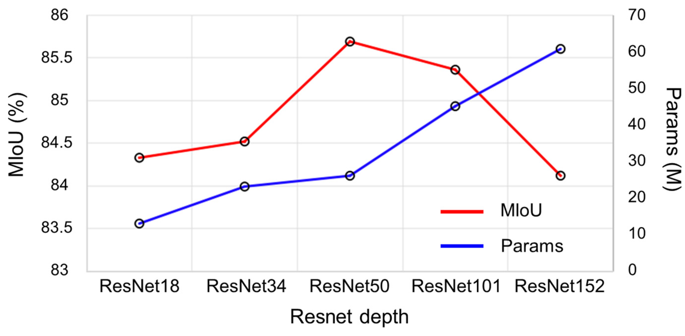
Figure 13 shows how the model performs as the encoder depth increases. The number of parameters rises with an increase in the number of network layers. Resnet50 has the highest MIoU at 85.69%, and Resnet152 has the lowest MIOU at 84.12%, a difference of 1.57%. This indicates that although the residual network can suppress the invalid convolutional layers through the residual connections, the suppression effect has its limitations, and an optimal number of layers exists. If the number of layers is below the optimal number, features cannot be fully extracted. Conversely, if the number exceeds the optimal amount, overfitting occurs. Thus, selecting an appropriate encoder depth is crucial for optimal performance.
5.3. Learning Rate Adjustment Strategy
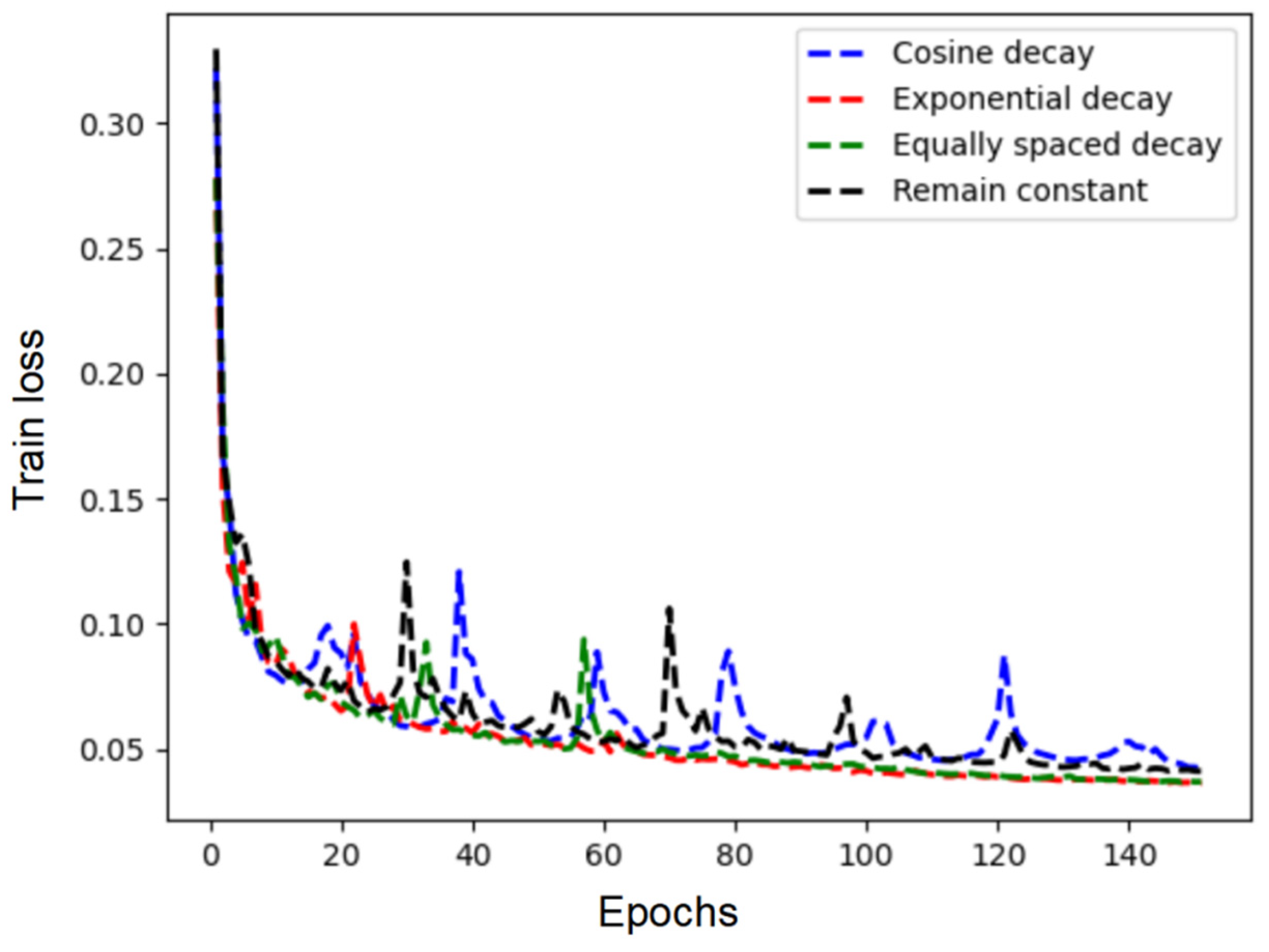
MobileNet_v2 was used as the encoder for the subsequent study, and four learning rate adjustment strategies were applied: Remain constant, Cosine decay, Equally spaced decay, and Exponential decay. These strategies were tested using Adam Optimizer. The metrics of different learning rate adjustment strategies are shown in
Table 7. Exponential Decay achieved the highest MIoU (87.14%), while the strategy with no attenuation (Remain Constant) resulted in the lowest MIoU (86.07%), a difference of 1.07%.
Figure 14 illustrates how the training loss (i.e., the value of the loss function) changes as the epoch increases. Equally spaced decay and exponential decay demonstrate the most stable training processes, reaching the lowest losses at final training. Conversely, the training losses associated them with remain constant, and cosine decay strategies exhibit considerable fluctuations. These fluctuations are likely attributable to the excessive learning rate, which causes the model parameters to oscillate around the extrema. This suggests that, despite the adaptability of the Adam optimizer in adjusting the learning rate, implementing step length attenuation remains essential for achieving optimal performance.
5.4. Loss Function and Data Imbalance
In this study, CE, WCE, and Focal Loss were used as loss functions to assess their effects on an unbalanced dataset, with CE serving as the standard for comparison.
Table 8 presents the metrics of models using different loss functions. Notably, the MPA value for WCE and Focal Loss is lower than that for CE, while the MPR is higher. Additionally, the MIoU for WCE and Focal Loss is approximately 3% lower than that for CE. This decrease can be attributed to the introduction of weight factors in WCE and focal factors in Focal Loss. These adjustments can mitigate the impact of data imbalance by reducing the emphasis on the dominant classes, thus potentially improving the recall for target categories. However, this improvement is relatively tiny for MPR. Generally, the WCE and Focal Loss lead to more misclassifications of other object types as target ground objects, which significantly diminishes the MPA. Consequently, the MIoU experiences a noticeable decrease. In summary, both WCE and Focal Loss fail to achieve the objective of enhancing segmentation accuracy on the unbalanced dataset. Despite attempts to address class imbalance through modified loss functions, the overall performance remains suboptimal compared to using traditional Cross-Entropy loss.
5.5. Input Image Size
Different sizes of input images are vital for optimizing model performance (
Table 9). The 512 × 512 size has the best performance, achieving an MIoU of 87.14%, while the remaining sizes hovered around 85–86%. Generally, larger image sizes offer more information to the model, aiding in pixel category prediction. However, distant information may be irrelevant and could potentially interfere with the model’s classification judgment. This likely explains why the 1024 × 1024 size yielded lower prediction accuracy compared to the 512 × 512 image size. Additionally, the size of the model’s receptive field is crucial. The study uses a receptive field of 512 × 512, which may also contribute to the superior performance of the 512 × 512 size images.
For segmentation accuracy across different categories, the 512 × 512 image size excelled in cloud and snow segmentation, likely due to its ability to capture relevant details effectively. However, for lakes, the 1024 × 1024 input size demonstrated superior accuracy. This suggests that larger objects, such as lakes, require a more comprehensive representation. The 1024 × 1024 size provides the network with more relevant information, which the 512 × 512 size image may not fully capture.
In conclusion, selecting the appropriate input size involves considering the size of the target object. Input sizes that are too small may hinder the model’s ability to capture all features accurately, while excessively large sizes may introduce noise, reducing prediction accuracy. Moreover, different input sizes impose varying requirements on the model’s receptive field, necessitating the selection of a suitable network structure tailored to the input size.
5.6. Bands Combinations
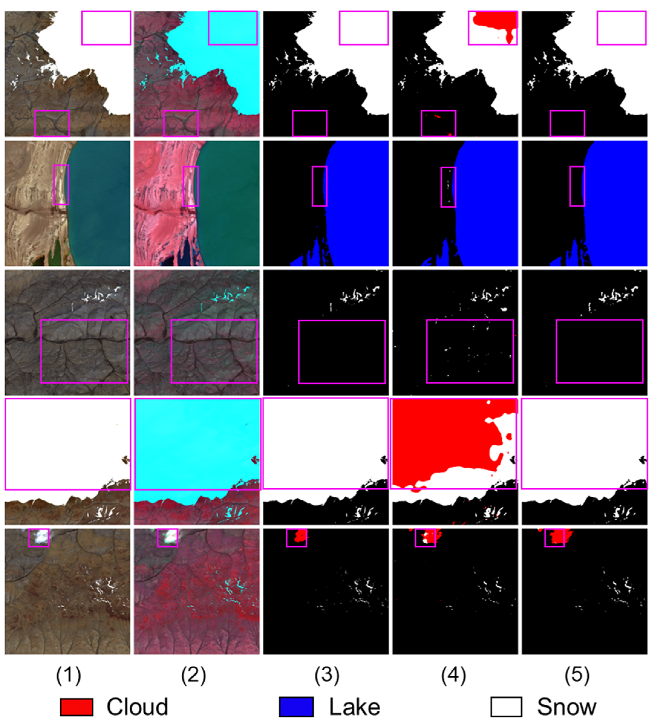
In this part, images synthesized in bands 4-3-2 (true-color image), 11-3-2 (false-color image), and 12-3-2 (false-color image) were input into the neural network. Results are shown in
Table 10. The MIoU for bands 12-3-2 was the highest at 87.14%, followed closely by the 11-3-2 bands at 86.65%. The MIoU for the 4-3-2 bands was the lowest at 82.28%. Since the 12-3-2 bands were selected for the initial settings, the parameter settings were configured accordingly. This primarily resulted in a slightly higher MIoU metric for the 12-3-2 bands compared to the 11-3-2 bands. However, different wavelengths within the SWIR band (i.e., bands 11 and 12) present slight discrepancies. Moreover, there was a significant difference in the results between the 12-3-2 bands and the 4-3-2 bands. The IoU for lakes was similar in both cases (i.e., bands 12-3-2 and 4-3-2), approximately 95%. However, the IoU for clouds and snow in images of bands 4-3-2 was significantly lower, by 7.82% and 11.63% lower, respectively, compared to images of bands 12-2-3.
Figure 15 shows images synthesized using different bands along with their predicted segmentation outputs for clouds, snow, and lakes. Notably, when utilizing the true-color image (bands 4-3-2), significant confusion between clouds and snow is evident. Specifically, central regions of snow are often erroneously detected as clouds, while cloud edges are mistakenly identified as snow. Moreover, background pixels frequently undergo misclassification as snow. Due to the presence of salt-out crystals or sand with spectral and texture properties similar to snow, lakes are often incorrectly classified as snow. Fortunately, the incorporation of SWIR bands (i.e., bands 11 and 12) substantially aids in distinguishing between clouds and snow.
6. Discussion
Clouds and underlying surfaces often share similar spectral characteristics, posing challenges for accurate cloud recognition due to their susceptibility to noise interference. Effective noise reduction is critical to enhancing precision in cloud recognition. Lakes, characterized by low reflectance in the visible light range, are relatively straightforward to segment. In contrast, clouds and snow present difficulties due to their similar spectral and textural features in the visible light range. To mitigate this, we introduce the SWIR bands, which significantly enhance discrimination between clouds and snow. Notably, different SWIR bands yield similar segmentation results. Some post-processed features, such as Normalized difference vegetation index (NDVI), Normalized difference water index (NDWI), and Normalized difference snow index (NDSI), may offer more direct guidance for the segmentation of snow and clouds. However, we chose not to use them as inputs, as they would interfere with the performance evaluation of the original bands in neural networks, which is the primary objective of this study. Given the considerable size variations among clouds, snow, and lakes, as well as variations within each category, multi-scale feature fusion becomes imperative in model simulation. The FPN employed in this study effectively integrates features across diverse receptive field sizes, facilitating accurate identification of objects at varying scales. Consequently, this model exhibits enhanced performance in the recognition of clouds, snow, and lakes.
The multi-head self-attention mechanism of the Transformer, employed by the Mit_b5 encoder, is currently a focal point of research. This mechanism excels at capturing global information, a task that CNN struggles with. However, in our study focusing on segmenting clouds, snow, and lakes, the Transformer did not perform as effectively. Two primary reasons account for this discrepancy. Firstly, the Transformer architecture requires a significant number of parameters, necessitating a large dataset for effective model training. The number of datasets utilized in our study did not meet these requirements. Secondly, the segmentation tasks in our study are relatively straightforward, requiring primarily local information rather than extensive global context. Overemphasis on global information may introduce noise, thereby reducing the accuracy of model predictions.
The introduction of residual structures in encoders such as ResNet50, ResNext50, and MobileNet_v2 significantly accelerates model convergence and enhances prediction accuracy compared to direct convolution (i.e., Vgg19) (
Table 6). Incorporating a depth-separable structure within the residual block not only reduces the number of parameters but also improves prediction accuracy. More parameters do not necessarily equate to better performance. Simple tasks often achieve superior results with streamlined structures and fewer parameters. In the experiment on encoder depth, MIoU initially increased with deeper encoders and more parameters but then plateaued and eventually decreased (
Figure 13). This change indicates that large parameter counts and deep encoder layers (i.e., large size of receptive fields) are not universally beneficial; instead, the optimal configuration depends on the specific task. While the Adam optimizer dynamically adjusts learning rates using a gradient (e.g., first and second moments), our experiment reveals the necessity of incorporating learning rate decay to achieve superior results (
Table 7). Learning rate decay aids the model in converging more effectively towards global or local optima, thereby enhancing prediction accuracy. Efforts to address data imbalance in clouds, snow, and lake segmentation using WCE and Focal Loss did not yield anticipated improvements. While WCE and Focal Loss alleviate the challenges of target classification, they introduce additional noise, leading to decreased prediction accuracy. This result may be attributed to suboptimal settings of weight and focus factors or inherent differences in multi-classification challenges. In binary classification tasks, WCE and Focal Loss might perform better.
Regarding the setting of the input image size, the experiments were conducted with optimal model parameters based on a receptive field size of 512 × 512. Consequently, it is expected that the 512 × 512 image size performs best. Generally, the choice of input image size should align with the size of the target objects. A too-small image size may limit the model’s ability to learn effective features, whereas an excessively large size can introduce unnecessary noise that hampers training. Ideally, with sufficient video memory, larger input image sizes are beneficial, as they provide more information for the model to use when predicting pixels. However, not all of this additional information is useful; some might introduce noise that interferes with predictions. Adjusting the model’s structure helps define an appropriate receptive field for the task, thereby specifying the scope of reference information used in predicting pixel categories, and mitigating noise interference enhances overall prediction accuracy.
The performance of the model is influenced by multiple factors, each impacting simulation results to varying degrees. The model structure, encoder choice, and input bands notably affect performance, with differences in MIoU indices exceeding 5% across different parameter configurations. In contrast, factors such as learning rate decay strategy, loss function selection, and input image size have a relatively minor impact on performance. These findings provide valuable insights for optimizing model parameters, offering a useful reference for future research and applications in semantic segmentation.
Few previous studies have comprehensively evaluated the factors influencing neural network performance in detecting clouds, snow, and lakes. Qiu et al. (2019) employed the Function of mask (Fmask) 4.0 algorithm to detect clouds and cloud shadows, which improved the overall segmentation accuracy. However, this approach is limited to small-scale regions and is less effective for large-scale areas like TP. Zhong et al. (2022) explored using a neural network to extract lake water bodies using public datasets. We believe that public datasets may not be suitable for all regions, and creating labels specific to the study area will likely enhance model performance. The performance of various neural networks and their structural innovation is a primary objective in the field of semantic segmentation [
17,
19,
20]. Xia et al. (2020) proposed a novel multi-scale feature extraction structure, demonstrating its effectiveness and crucial role in the extraction of clouds, snow, and lakes, which is consistent with the findings of this study. Transformer, combined with CNNs, has been proven effective in semantic segmentation tasks in previous studies [
15]. However, our research yielded contrary results. This discrepancy may be attributed to the dataset not being large enough, among other factors that warrant further exploration in future research.
7. Conclusions
This study investigates the factors influencing neural network algorithm performance in detecting clouds, snow, and lakes in Sentinel-2 images. Key contributions and findings include the following:
(1) A two-stage classification algorithm based on spectral features was developed using Sentinel-2 images. This algorithm effectively reduces the interference from spectral similar pixels between classes, ensuring accurate pixel classification.
(2) FPN was identified as the most effective model structure due to its ability to integrate features from different receptive field sizes, improving the recognition of objects with varying scales. Encoders with residual structures, such as ResNet50 and MobileNet_v2, showed better performance. The introduction of the SWIR band significantly improved the distinction between clouds and snow. Larger input image sizes did not necessarily yield better results due to potential noise interference.
(3) Model architecture, encoder type, and different band combinations were found to have the most substantial impact on performance, with variations in these parameters resulting in IoU differences of over 5%. Learning rate decay strategy, loss function, and input image size also influence performance, though their impact is relatively smaller.
While this study primarily investigates factors influencing semantic segmentation of clouds, snow, and lakes in plateau mountain regions, its findings provide insights applicable to various surface objects in remote sensing images. The conclusions offer valuable guidance for optimizing neural network parameters and structures tailored to remote sensing image segmentation. These insights are particularly pertinent for applications dealing with substantial object-scale variations and data imbalance.
