Article

Efficient Jamming Policy Generation Method Based on Multi-Timescale Ensemble Q-Learning

1
College of Electronic Engineering, National University of Defense Technology, Hefei 230037, China
2
Unit 93216 of PLA, Beijing 100085, China
*
Author to whom correspondence should be addressed.
Remote Sens. 2024, 16(17), 3158; https://doi.org/10.3390/rs16173158
Submission received: 26 June 2024 / Revised: 23 August 2024 / Accepted: 25 August 2024 / Published: 27 August 2024

Abstract

:
With the advancement of radar technology toward multifunctionality and cognitive capabilities, traditional radar countermeasures are no longer sufficient to meet the demands of countering the advanced multifunctional radar (MFR) systems. Rapid and accurate generation of the optimal jamming strategy is one of the key technologies for efficiently completing radar countermeasures. To enhance the efficiency and accuracy of jamming policy generation, an efficient jamming policy generation method based on multi-timescale ensemble Q-learning (MTEQL) is proposed in this paper. First, the task of generating jamming strategies is framed as a Markov decision process (MDP) by constructing a countermeasure scenario between the jammer and radar, while analyzing the principle radar operation mode transitions. Then, multiple structure-dependent Markov environments are created based on the real-world adversarial interactions between jammers and radars. Q-learning algorithms are executed concurrently in these environments, and their results are merged through an adaptive weighting mechanism that utilizes the Jensen–Shannon divergence (JSD). Ultimately, a low-complexity and near-optimal jamming policy is derived. Simulation results indicate that the proposed method has superior jamming policy generation performance compared with the Q-learning algorithm, in terms of the short jamming decision-making time and low average strategy error rate.

1. Introduction

With the rapid development of information technology, the electromagnetic environment of modern battlefields has become increasingly complex, and the role of electronic warfare has become more critical [1]. As a crucial part of electronic countermeasures, the goal of interference decision-making is to generate the optimal interference strategy in real-time based on threat perception and judgment of radar signals, thereby effectively completing the task of interfering with radar and reducing the threat of enemy radar [2]. Driven by advanced electronic technologies, such as digital phased array systems, radar is gradually evolving toward multifunctionality. For example, it has the ability to quickly change the waveform between pulses and can adaptively adjust the working state according to the task and external environment [3,4,5,6,7].
Currently, multifunctional phased array radar (MFPAR) has advantages, such as fast response speed, flexible beam control, strong anti-interference ability, and can achieve various functions, such as search, tracking, recognition, and guidance through multi-dimensional parameter regulation. Due to the inability to directly obtain changes in the radar operating status, it poses great challenges to the jamming decision-making of the jammer. If the jammer lacks sufficient prior knowledge of the radar state, it will be difficult to establish the optimal correspondence between the radar state and existing jamming styles, and thus impossible to form an optimal jamming strategy for different radar states. Therefore, it is of great significance to study efficient jamming strategy generation methods for MFPAR with complex systems.

1.1. Cognitive Radar Countermeasure Process

Electronic warfare (EW) is crucial in modern warfare for gaining electromagnetic superiority, which aims to control the electromagnetic spectrum by attacking enemy electronic systems while protecting friendly ones [2,8,9,10]. Traditional adaptive electronic warfare employs pre-set or environmentally adaptive countermeasures to respond to enemy electronic systems, which relies heavily on human expertise without the capability for reasoning and learning. The emergence of cognitive electronic warfare (CEW) can improve the rapid response capability and reliability of jammers [11,12,13,14]. CEW perceives enemy signals through prior knowledge and interactive learning, and then uses artificial intelligence algorithms to quickly generate optimal jamming decisions [15,16,17,18,19]. Figure 1 illustrates the cognitive radar countermeasure process, where cognitive jamming, cognitive reconnaissance, cognitive evaluation, and the target environment form a closed loop [20,21].
Combining cognitive theory with jamming decision-making concepts to form a cognitive-based jamming decision system will significantly enhance the accuracy and real-time capabilities of jamming and meet the need for effective jamming against advanced MFR. Therefore, the jamming decision system must be capable of real-time selection of the optimal jamming strategy based on the reconnaissance-obtained parameters of the radar. It should utilize an evaluation module to assess jamming effectiveness in real-time and adjust the jamming strategy accordingly. Thereby, it forms a closed-loop system from jamming application to real-time feedback, which aligns with the real-time and dynamic requirements of CEW.

1.2. Traditional Jamming Strategy Generation Methods

Researchers have extensively studied jamming decision-making from three aspects: template matching, game theory, and reasoning algorithms [22,23]. Nonetheless, these techniques significantly depend on extensive pre-existing knowledge, which poses a strong challenge when trying to adjust to the swiftly evolving and intricate electromagnetic environment. The template-matching method compares radar signal samples with those in a template library and selects the jamming pattern corresponding to the most similar sample. This approach is mainly suitable for radars with fixed and unchanging parameters, and the quality of the template library directly affects the accuracy of jamming decisions. However, it lacks timeliness and often lags behind the rapidly changing battlefield environment [24]. The game theory method treats the radar and jammer as two players in a game, where the strategy set and payoff matrices are defined. The jammer picks a jamming pattern from the available strategy set and then obtains a payoff based on the payoff matrix. This method can optimize the selection of jamming patterns to a certain extent [25,26]. However, the game-theory-based jamming decision method is highly dependent on the payoff matrix, which also requires extensive expert experience for its construction and cannot guarantee real-time jamming of the radar. The reasoning algorithms examine past events to identify causal links, thereby estimating the likelihood of future events occurring under specific conditions and supporting jamming decision-making [26,27]. However, this method also lacks real-time capability, and the easily accumulated errors will affect the accuracy of jamming decisions.
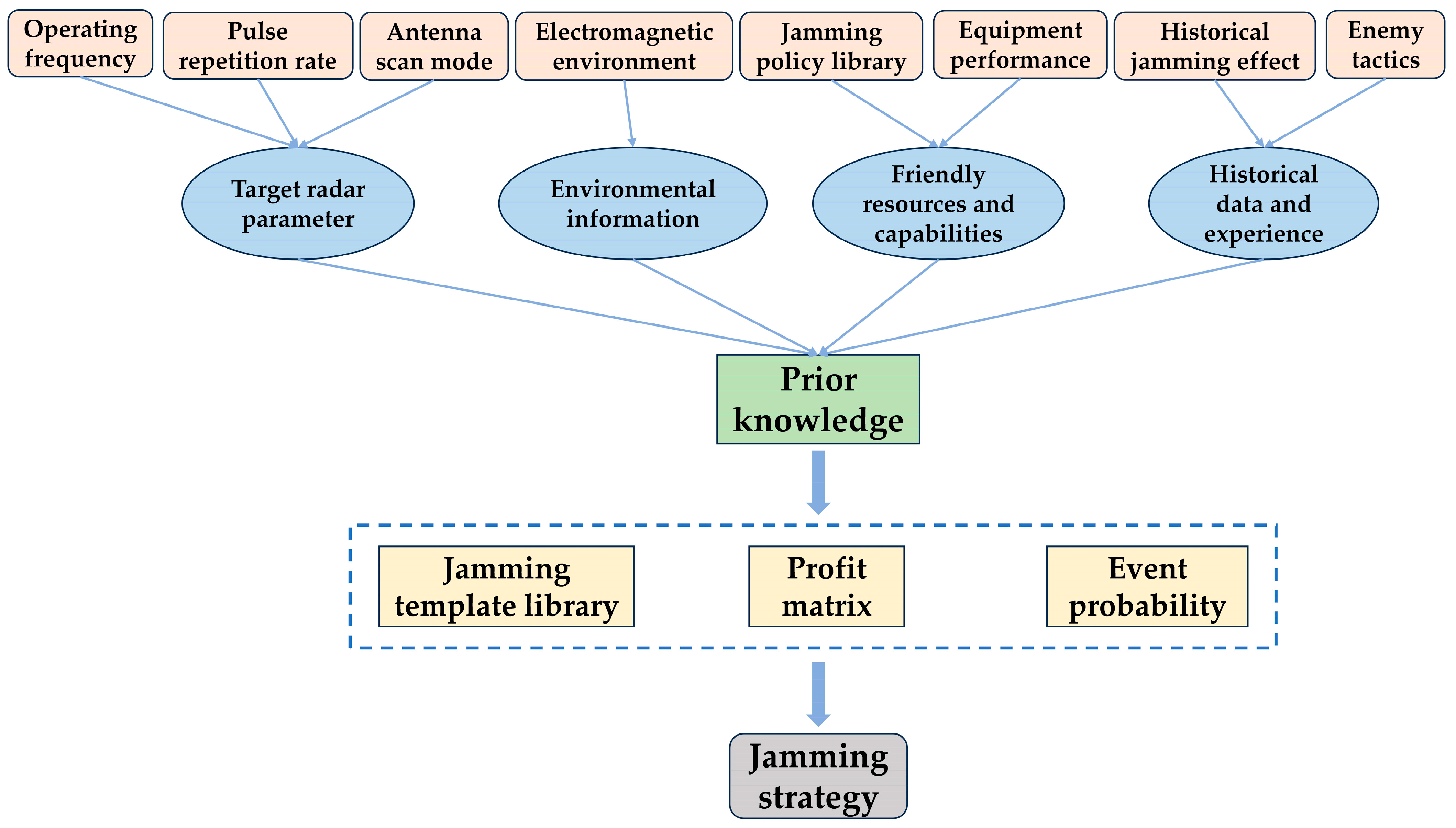
The three aforementioned methods can play a role in jamming decision-making to some extent. However, it is challenging to obtain prior information for new system radars, such as MFR, which makes it difficult for accurate jamming in actual combat. As shown in Figure 2, the prior knowledge refers to the information about the electromagnetic environment and target radar, which is already known before making jamming decisions. This includes the operation parameters of the target radar, environmental information, friendly resources and capabilities, historical data, and experience. This prior knowledge influences the jamming template library, the payoff matrix, and the calculation of event probabilities after taking different jamming measures, ultimately affecting the generation of jamming strategies.

1.3. Jamming Strategy Generation Methods Based on Reinforcement Learning

To develop a strategy for jamming that effectively counters MFRs, it is meaningful to explore an efficient jamming decision-making approach that does not rely on prior data. The advent of reinforcement learning addresses the shortcomings of traditional jamming decision-making methods that overly depend on prior data [28]. Popular reinforcement learning algorithms encompass methods such as temporal difference (TD), policy gradient, Q-learning, and SARSA [29,30,31]. Additionally, researchers have proposed improvements to these algorithms to address issues, such as high noise sensitivity and large estimation biases [32]. Llorente et al. provided a comprehensive overview of the application of Monte Carlo methods in noisy and costly densities and applied them to reinforcement learning and approximate Bayesian computation (ABC) [33]. Liu, W. et al. utilized the Q-ensemble approach to derive optimal policies from static datasets, employing techniques such as large-batch punishment and binary classification networks to differentiate in-distribution from out-of-distribution data, thereby reducing the Q-ensemble size and enhancing the performance and training speed [34]. Essentially, reinforcement learning entails an interaction between the agent and its environment, wherein the agent adapts its strategy according to the rewards received from its actions, aiming to maximize future rewards.
The concept of cognition was first introduced into the field of radar electronic warfare in [35], which applies the Q-learning algorithm to the cognitive radar countermeasure process. The authors of [36] developed a cognitive jamming decision-making system, concentrating on the creation of jamming strategies and the evaluation of their effectiveness. The authors of [37] improved the jamming decision problem model by modeling the problem as a Markov decision process with rewards. The authors of [38,39,40,41] improved the Q-learning algorithm significantly by enhancing the decision-making efficiency and reducing the training time. To handle larger radar state spaces, the authors of [42,43,44] employed deep reinforcement learning techniques to address the jamming decision problem, which significantly enhanced the efficiency and accuracy of jamming decisions within high-dimensional state spaces. The authors of [45] introduced a method for generating jamming strategies using heuristic planning combined with reinforcement learning. This method constructs a heuristic reward function using a potential function, which improves sample utilization while reducing sample complexity and shortening the jamming decision time. The authors of [46,47,48,49] began to consider various radar countermeasure scenarios, which addressed different issues, such as optimal jamming parameter selection and multi-agent jamming systems.
To address issues such as low jamming efficiency and accuracy against advanced MFRs, an efficient jamming policy generation method based on multi-timescale ensemble Q-learning is proposed in this paper. The main contributions of this paper are summarized as follows:
  • A realistic radar countermeasure scenario was established, in which an aircraft carries a jammer for self-protection to avoid being locked by radar during mission execution. The transition modes of the MFR operating modes were analyzed, and mode-switching rules were designed for scenarios both with and without jamming.
  • The problem of generating jamming strategies was modeled as a MDP, with the goal of identifying the optimal jamming strategy in the dynamic interaction between the MFR and the jammer.
  • An efficient jamming strategy generation method based on MTEQL was proposed. First, the adversarial process between the radar and the jammer was sampled to construct multiple structurally related Markov environments. The Q-learning algorithm was then run in parallel across these environments. A JSD-based adaptive weighting mechanism was employed to combine the multiple output Q-values, ultimately obtaining the optimal jamming strategy.
  • Numerical simulations and experimental investigations were carried out to demonstrate the effectiveness of the proposed method. Results highlighted that the proposed method achieved faster jamming strategy generation and higher decision accuracy.
The primary structure of this paper is outlined as follows: Section 2 designs the radar countermeasure scenario and models the jamming strategy problem, Section 3 proposes the jamming strategy generation algorithm, Section 4 presents the simulation experiments, and Section 5 provides the conclusions.

2. Radar Countermeasure Scenario Design and Problem Modeling

2.1. Radar Countermeasure Scenario Design

This paper discusses a scenario in which an aircraft carries a jammer for self-protection, releasing jamming signals to avoid being locked by a MFR during missions. The focus is on the one-on-one confrontation between the jammer and the radar, as illustrated in Figure 3. The MFR on the fighter jet tracks the target aircraft, which is equipped with a jammer capable of intercepting radar signals in real time for reconnaissance. The jammer evaluates the effectiveness of its jamming based on changes in the intercepted radar signals. Through continuous confrontation with the radar, the jammer learns the radar’s mode transition patterns and jamming strategies. It then selects the optimal jamming method based on these strategies and releases jamming signals accordingly. The goal of the jammer is to continuously reduce the threat level posed by the radar’s operational modes, thereby protecting the target from being locked by the radar.
At the present time step, the jammer detects that the MFR is in state s t . The jammer obtains a reward, r t , based on the transformation of the radar state. After updating its jamming strategy, it employs jamming pattern a t to jam with the MFR. As a result of the jamming, the radar state transitions to s t + 1 . The jammer detects the change in the radar state and obtains another reward, r t + 1 . The jammer then updates its policy and makes a new decision, iterating this process continuously. Based on the above analysis, the task of generating jamming policies is essentially a sequential decision-making problem, which can be modeled using the MDP. The MDP is described by the tuple { S , A , P , R } , in which S, A, P, and R represent the radar states, jamming patterns, radar state transition probabilities, and immediate rewards, respectively.

2.2. Radar Operation Mode Modeling

To effectively jam the MFR, it is crucial to accurately model its operational modes. Such modeling not only enhances the understanding of the radar’s performance across different modes but also provides a theoretical foundation for developing effective jamming strategies.
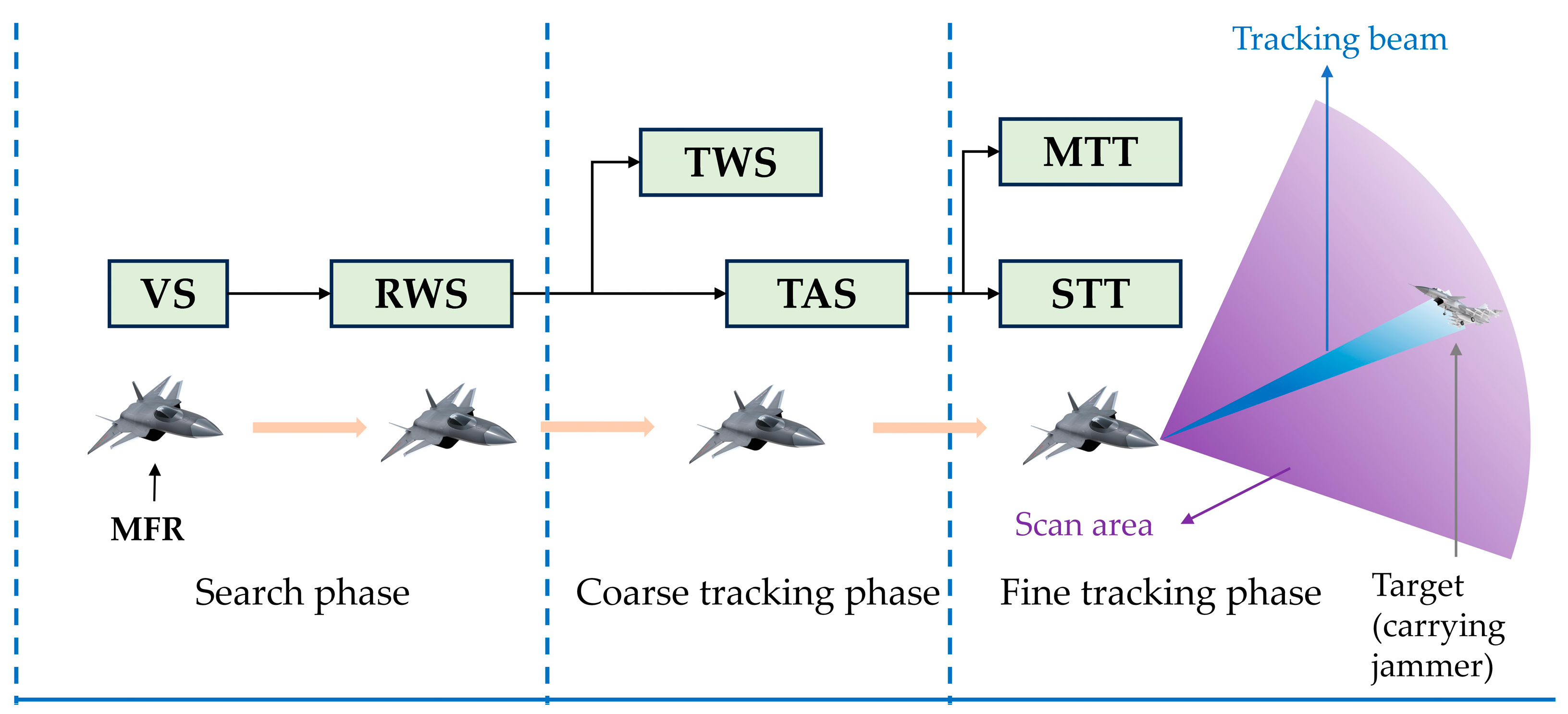
The state space, denoted as S = [ s 1 , s 2 , , s N ] , comprises various operation modes of the multi-function radar (MFR), totaling N modes. The MFR can operate in several modes, including velocity search (VS), range while search (RWS), track while scan (TWS), track and scan (TAS), multi-target track (MTT), and single-target track (STT). These operation modes can be flexibly switched. This paper designed the switching rule of the MFR’s operation modes in the absence of jamming, based on changes in the target’s threat level or distance, as shown in Figure 4.
When a fighter jet equipped with a MFR is at a considerable distance from the target and has not yet detected it, the radar initially operates in VS mode, conducting a comprehensive search of the mission area. At this stage, the threat level is minimal, as no target has been detected. Upon detecting a target, the MFR switches to RWS mode to continue tracking the target, taking into account resource constraints. As the target approaches, the MFR enters the coarse-tracking phase, with the fighter jet selecting either TWS or TAS mode based on real-time conditions. When the fighter jet is very close to the target and the threat level is high, the radar transitions to STT or MTT mode, entering a continuous fine-tracking phase. This phase provides robust support for subsequent precise weapon strikes. Consequently, the threat level is highest at this stage, and jamming efforts must focus on preventing the MFR from operating in this mode.
The action space consists of various jamming patterns, denoted as A = [ a 1 , a 2 , , a M ] , with a total of M patterns. These include narrowband noise jamming (NNJ), wideband noise jamming (WNJ), swept-frequency noise jamming (SFNJ), comb spectrum jamming (CSJ), dense false-target jamming (DFTJ), slice repeater jamming (SRJ), range gate pull-off jamming (RGPJ), velocity gate pull-off jamming (VGPJ), and doppler noise jamming (DNJ). These patterns are primarily categorized into three types: blanket jamming, deception jamming, and combined blanket–deception jamming. Each type exerts distinct effects on the radar, and successful jamming can reduce the threat level of the MFR’s operational modes.
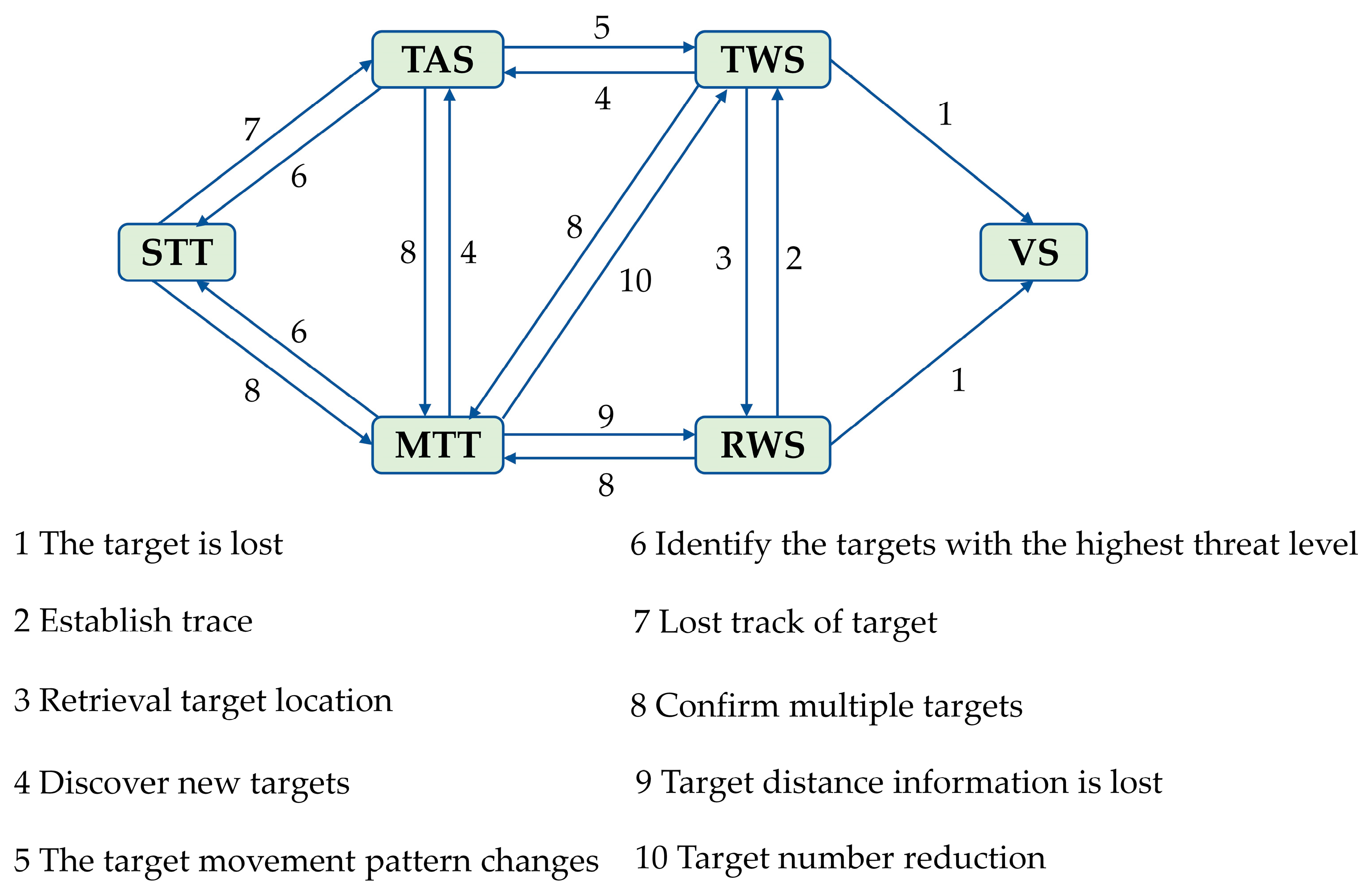
The state transition probability, p ( s t + 1 | s t , a ) , represents the likelihood of the radar transitioning from state s t to state s t + 1 after being subjected to jamming. Changes in the external electromagnetic environment can cause shifts in the radar’s operational modes, with the switching rules for these modes illustrated in Figure 5. Different types of jamming have varying effects on the radar’s mode transitions, and selecting effective jamming can reduce the threat level of these modes. For instance, when the radar is operating in TWS mode and subjected to RGPJ, the target position changes, prompting the radar to re-acquire the target and switch to RWS mode. If the radar encounters SFJ and detects a new target, it can still switch to TAS mode, and if multiple targets are confirmed, it can transition to MTT mode. When subjected to NNJ, if the target is successfully suppressed, the radar loses the target and needs to search again, thus switching to VS mode.
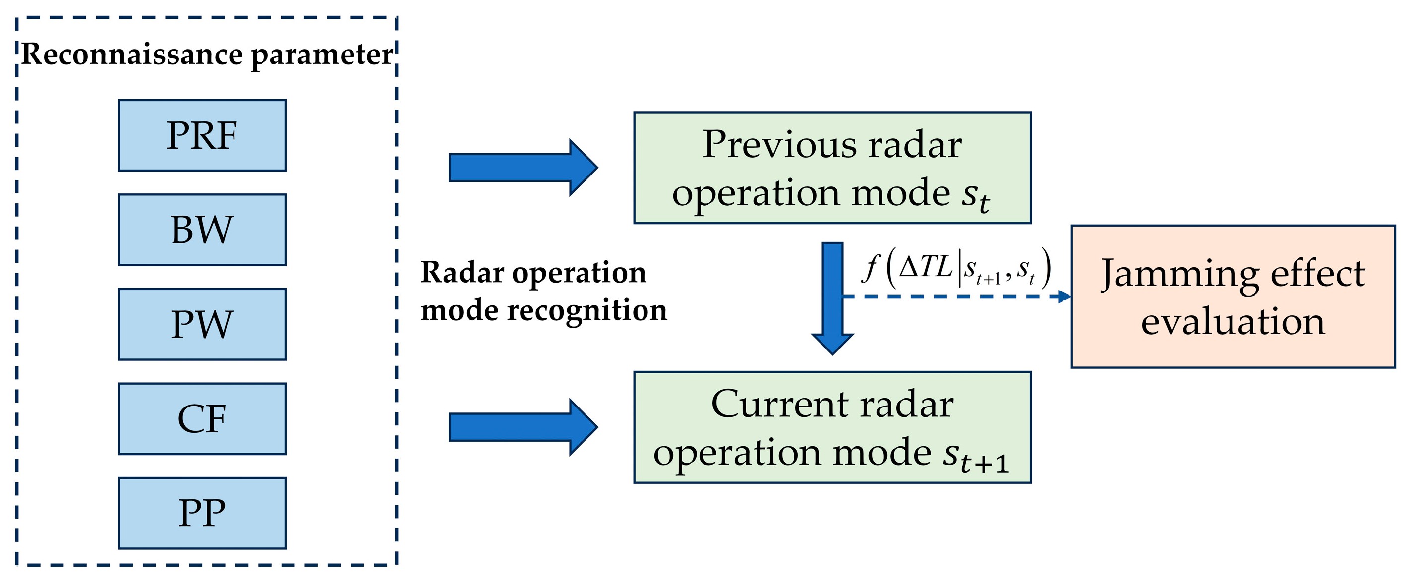
Online jamming effectiveness assessment, a critical component in the closed-loop generation of jamming strategies, has always faced significant challenges. Accurately evaluating jamming effectiveness requires real-time processing of complex electromagnetic environment data and considering the dynamic response and adaptive changes of the target radar. This evaluation process demands efficient algorithms and robust computational power to provide reliable feedback within a short timeframe, thereby optimizing the jamming policy. Since the jammer can intercept radar signals in real time and identify the radar’s state, and different radar states pose varying levels of threat to the jammer, it is possible to determine the effectiveness of the jamming in real time based on changes in the radar state. As shown in Figure 6, this paper defined the reward based on the changes in the radar state, where r ( s t + 1 | s t ) represents the reward obtained from the transition of the radar operation mode from s t to s t + 1 . The reward, r ( s t + 1 | s t ) , is the same as the jamming effectiveness evaluation value, r t , in Figure 3. In this paper, the effectiveness evaluation value was obtained based on the changes in the radar state observed after jamming. The current policy was adjusted and optimized according to the effectiveness evaluation value, ultimately identifying the optimal strategy that reduced the radar threat level the fastest. The difference in threat levels between two states is defined as:
Δ T L = T L ( s t + 1 ) T L ( s t ) .
Establishing a function, f , between the threat level difference and the reward, the reward, r ( s t + 1 | s t ) , is:
r ( s t + 1 | s t ) = f ( Δ T L | s t + 1 , s t ) .
The objective of this study was to minimize the threat level of the radar. Therefore, if the target threat level decreases, a positive reward is obtained, and the greater the decrease in the threat level, the higher the reward. Conversely, if the target threat level increases, a negative reward is received, and the greater the increase in the threat level, the lower the reward.

2.3. Problem Modeling

This paper modeled the problem of jamming policy generation as an MDP model. The core objective was to identify the optimal jamming pattern for each radar operation mode, ultimately transitioning the radar’s operation mode to the lowest threat level, i.e., finding the optimal jamming strategy, π : S A . After each jamming release, the jammer will perform an online evaluation of the jamming effectiveness, obtaining an instantaneous reward value, r a t ( s t ) . v π ( s ) is the value function under policy π , indicating the anticipated cumulative reward achieved by following the policy π from the initial state s , and its expression is given by the Bellman equation:
v π ( s ) = E π [ t = 0 γ t r a t ( s t ) | s 0 = s ] = E π [ r a t ( s t ) + γ v π ( s t + 1 ) | s 0 = s ] ,
where γ ( 0 , 1 ) represents the discount factor, which determines the importance of future rewards in current decision-making. The jammer’s objective is to solve the Bellman optimality equation to obtain the optimal policy as:
v * ( s ) = max π   v π ( s ) = max π   E π [ t = 0 γ t r a t ( s t ) | s 0 = s ] ,
π * ( s ) = arg max π   v π ( s ) ,
where v * is the optimal value function, and π * is the optimal policy. According to the aforementioned Bellman equation, solving the value function is a dynamic iterative process. Each state of the MFR can yield a value, and the continuous increase in the value function corresponds to the continuous optimization of the policy. Multiple different jamming actions can be executed for each radar state, resulting in the state–action value function, Q ( s , a ) . For the jammer, the state transition rules of the MFR are unknown. Through Q-learning, the jammer can learn these rules during the adversarial process with the MFR to solve for the optimal policy. By learning the value function, Q ( s , a ) , for each state–action pair ( s , a ) , the optimal policy can be found. The value function Q ( s , a ) is updated according to the following formula:
Q ( s , a ) Q ( s , a ) + α ( r a ( s ) + γ Q ( s , a ) Q ( s , a ) ) ,
where α ( 0 , 1 ) is the learning rate, representing the reward value obtained after performing action a in state s . Throughout the learning process, an ε -greedy policy was employed to balance exploration and exploitation, selecting a random action with a probability of ε and the current optimal action with a probability of 1 ε . Its greedy action selection strategy has similarities with simulated annealing and the Metropolis–Hastings algorithm in terms of balancing exploration and exploitation. The greedy action selection strategy in the ε -greedy algorithm is similar to the temperature control mechanism in simulated annealing, which includes a temperature parameter that initially allows for the acceptance of poorer solutions to avoid local optima [50]. As the temperature decreases, the algorithm increasingly favors greedy choices to achieve global optimality. The Metropolis–Hastings algorithm constructs a Markov chain by accepting or rejecting candidate states, with the acceptance probability proportional to the relative probability of the candidate state [51,52]. The ε -greedy strategy is akin to the acceptance probability strategy in the Metropolis–Hastings algorithm, particularly in introducing randomness to explore the state space. These algorithms introduce randomness and a gradual optimization strategy to avoid local optima, thereby increasing the probability of achieving a global optimum. The specific expression of the ε -greedy policy is shown as follows:
a = { arg max   Q ( s , a ) a ,   w i t h   a   probability   of   1 ε r a n d o m   selection ,   with   a   probabilty   of   ε .
The jammer interacts with the radar and collects samples { s , a , s , r } to update the Q ( s , a ) . The Q ( s , a ) eventually converges to the optimal value with probability 1, from which the optimal policy and value function can be derived as:
π * ( S ) = arg max a A   Q * ( s , a ) ,
v * ( s ) = max a A   Q * ( s , a ) ,
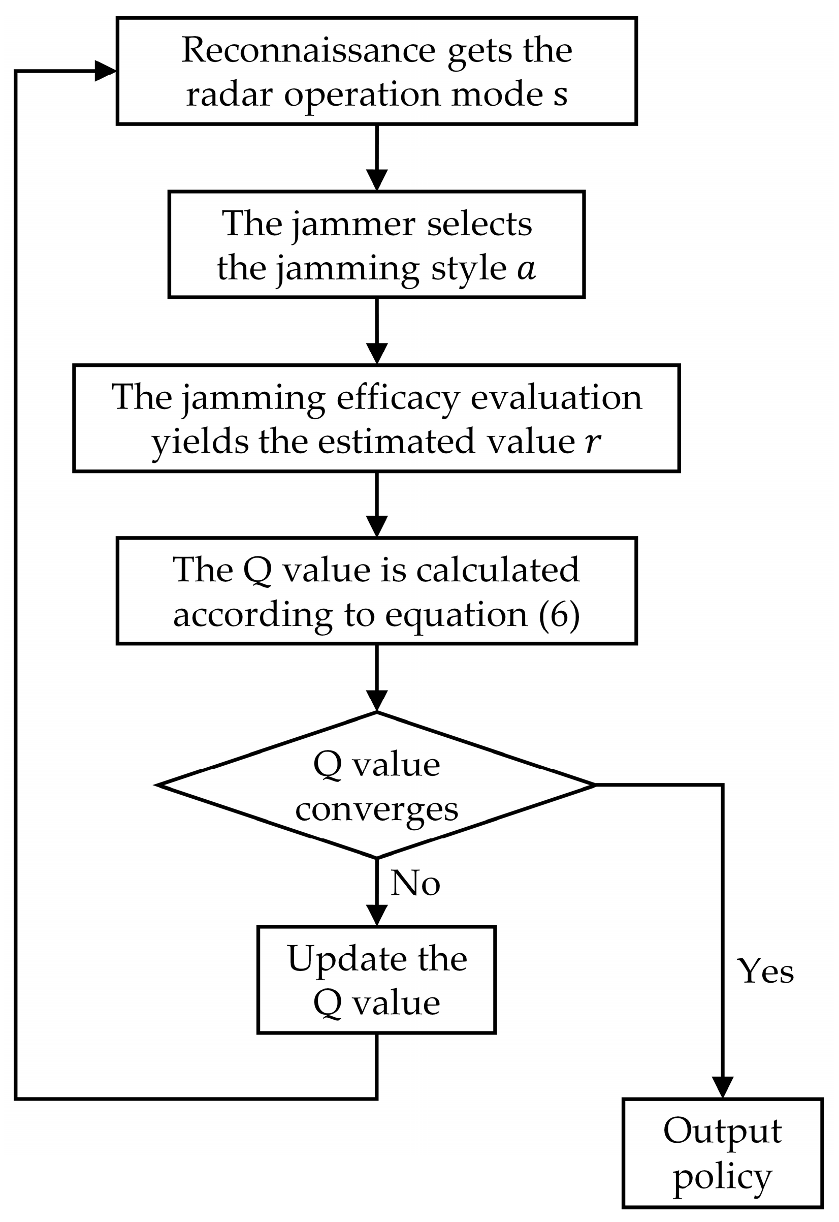
The jamming strategy generation algorithm table based on Q-learning is shown in Figure 7. The jammer detects the radar state and selects a jamming style. After obtaining the performance evaluation value, the Q-table is updated using Equation (1). The process iterates continuously, and after each Q-value calculation, it checks whether the Q-values have converged. If convergence is achieved, the optimal strategy is produced; if not, the process moves on to the next learning iteration.

3. Jamming Policy Generation Method Based on MTEQL

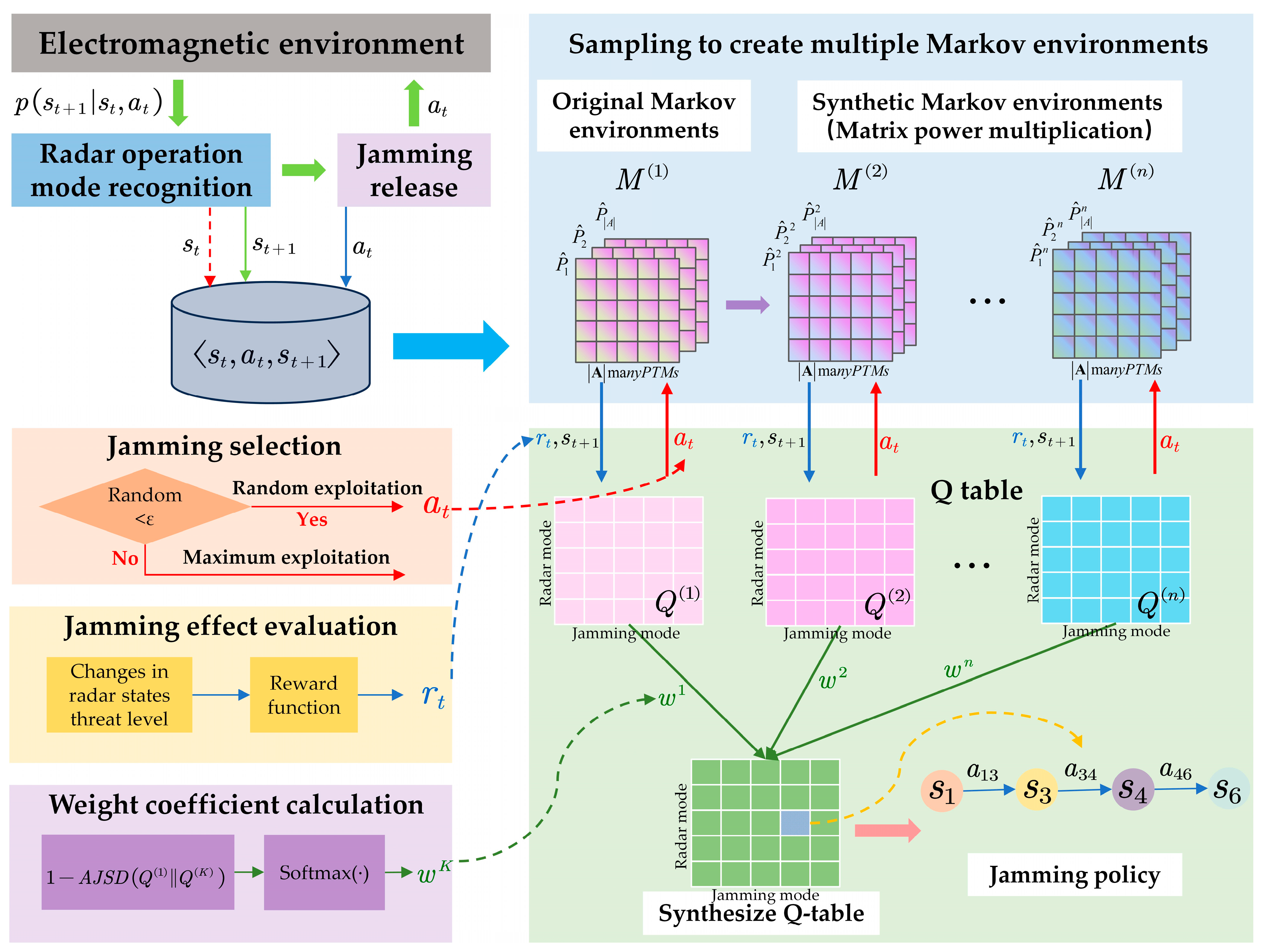
To enhance the efficiency and accuracy of jamming policy generation, this paper proposed an efficient jamming strategy generation method based on MTEQL [53]. The overall flowchart of the algorithm is shown in Figure 8, which primarily includes four parts: sampling to generate multiple Markov environments, jamming pattern selection, jamming effectiveness evaluation, and weight coefficient calculation. The jamming style selection was performed using a greedy method, the jamming effectiveness evaluation was based on the change in threat level of the radar operating mode before and after jamming, and the weight coefficients for each Q-table were calculated based on the JS divergence. The jamming style selection and jamming effectiveness evaluation were applied to the Q-table generated for each Markov environment. Finally, all Q-tables were combined into a composite Q-table using the calculated weight coefficients, and the optimal jamming strategy was obtained after the algorithm converged. The following sections will provide a detailed introduction to this method.
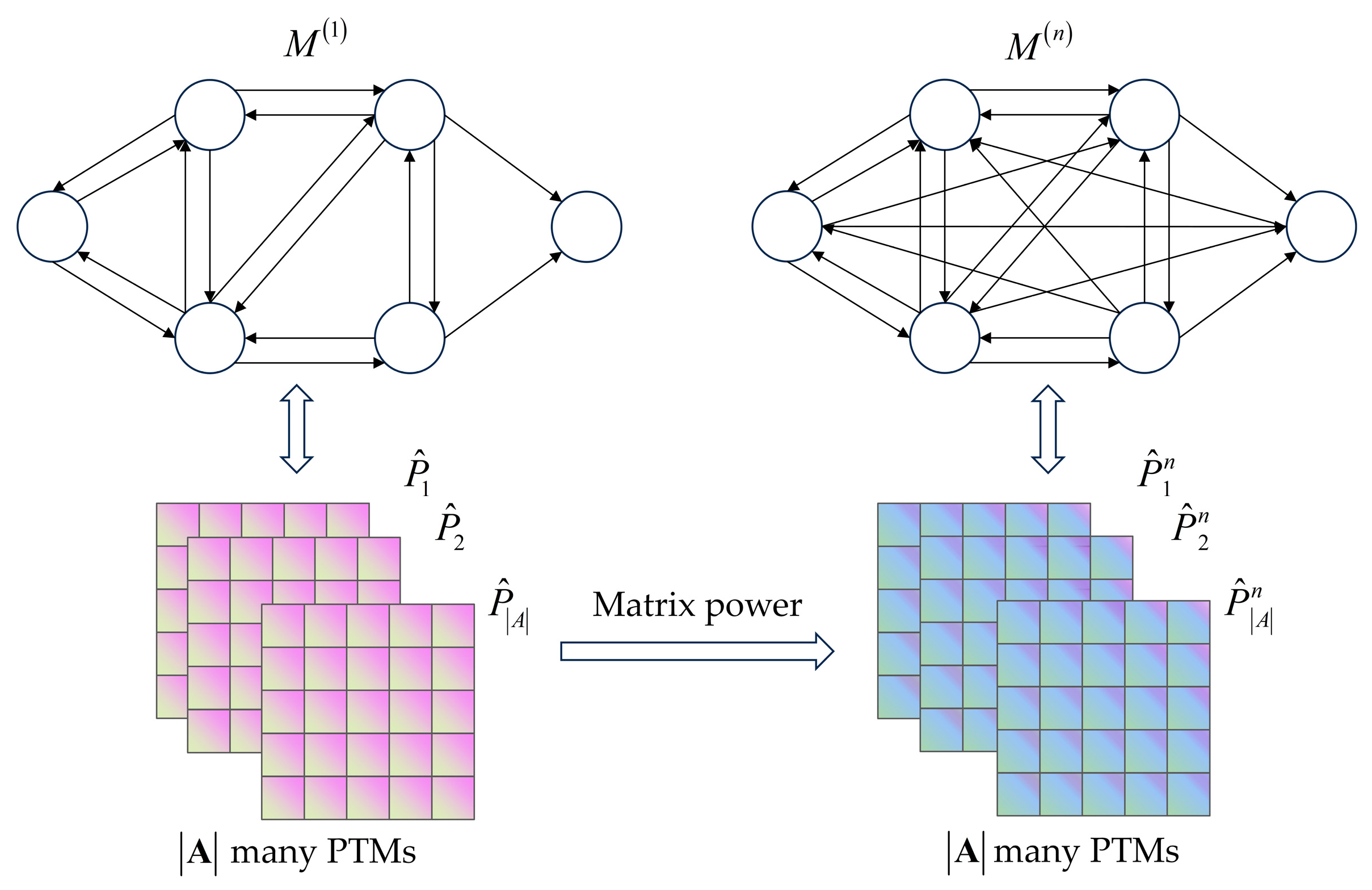
This method used an ε -greedy policy at the algorithm level and employed multiple structurally related Markov environments at the environment level to provide the jammer with radar state transition relationships over different time dimensions, thereby significantly enhancing the algorithm’s exploration capability in unknown environments. Different Markov environments correspond to different radar state transition probabilities, so the radar state transition probabilities are stored in a probability transition tensor (PTT), P , as Markov environments. P consists of | A | probability transition matrices (PTMs) of size | S | × | S | . First, approximate radar state transition matrices were obtained through sampling. Then, different Markov environments were generated by multiplying the original radar state transition matrices, constructing environments with multiple timescales that correspond to the n-hop transition matrices of the Markov chain. This approach enhanced the jammer’s exploration capability and accelerated the exploration phase of Q-learning.
Figure 9 illustrates the relationship between the original Markov environment and the synthesized Markov environment. Utilizing n-hop Markov environments can help the jammer better understand and adapt to the dynamically changing radar environment. Firstly, the jammer can accelerate its understanding of the environment by considering state transitions and reward signals over longer periods, discovering new valuable state–action pairs, and reducing unnecessary interactions with the radar. Secondly, n-hop Markov environments can simulate the potential trajectories of mode transitions that are not directly observable, allowing the jammer to learn the radar’s state transition patterns from indirect experiences.
The MTEQL algorithm uses the interactions between the jammer and the radar to obtain K Markov environments, including the original Markov environment and K-1 synthesized Markov environments. The difference between the MTEQL algorithm and the original Q-learning method is shown in the Figure 10. The MTEQL algorithm runs the Q-learning algorithm in parallel across multiple environments and finally merges the Q-functions obtained from different environments into a single Q-function estimate, resulting in an approximately optimal policy.
Algorithm 1 is the pseudocode for the jamming policy generation method based on MTEQL.
Algorithm 1 The pseudocode for the jamming policy generation method based on MTEQL
Input: Sampling path length,  l , the total number of Markov environments,  K , minimum number of times for each state transition pair,  v , training episodes,  E n u m , learning rate,  α , discount factor,  γ , replacement rate, ut, and Q-tables for K different environments,  Q ( n ) ,  n { 1 , 2 , 3 , , K } .
Output: The resultant Q-table,  Q i t , and jamming policy,  π ^ .
01. Initialize each element of P ^ a to 1 | S |
02. while the number of samples for ( s , s ) does not exceed v times do
03.          Randomly select an initial radar operation mode s
04.          repeat l times
05.                    The jammer obtains { s , a , s } after randomly applying jamming
06.                     P ^ a ( s , s ) P ^ a ( s , s ) + 1
07.          end
08. end while
09. Normalize the sum of each row in P ^ a to 1, and obtain M ( 1 ) through sampling
10. for n = 2,3, ,K do
11.          Compute the n t h power of the matrix to obtain P ^ a n
12.          Use M ( n ) to represent the synthesized Markov environment corresponding to P ^ a n
13. end for
14. Randomly initialize the weights w 0 , Q 0 i t 0 , t 0
15. for episode = 1,2, , E n u m do
16.          for n = 1,2, ,K do
17.                    Reconnaissance obtains the initial radar operation mode s 0
18.                    while  s s a i m  do
19.                              Select the jamming pattern a according to the ε -greedy policy
20.                              Obtain the next radar operation mode s from M ( n )
21.                              Obtain the reward r based on the radar state transition
22.                              Update Q t ( n ) using (5)
23.                    end while
24.                    Use SoftMax to convert Q t ( n ) to state probabilities Q ^ t ( n )
25.                     w t ( n ) 1 A J S D ( Q ^ t ( 1 ) Q ^ t ( n ) )
26.          end for
27.           w t s o f t max   ( w t )
28.           Q t + 1 i t u t Q t i t + ( 1 u t ) n = 1 K w t ( n ) Q t ( n )
29.           t t + 1
30. end for
31. π ^ ( s ) arg max a   Q i t ( s , a )
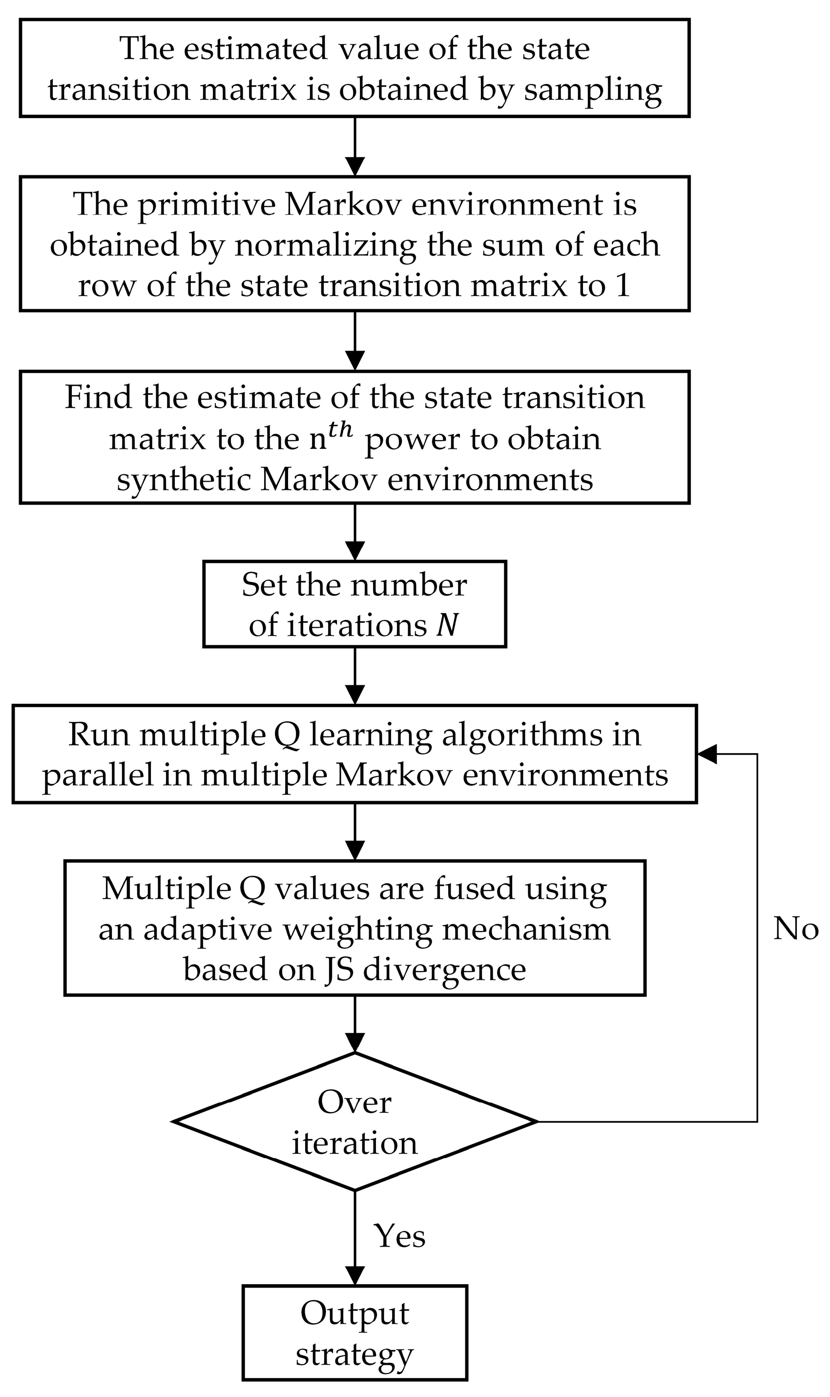
Since the jammer does not initially know the radar’s state transition matrix, it is necessary to sample the environment first and create multiple synthesized Markov environments. P ^ represents the estimated PTT, and P ^ a represents the PTM corresponding to each jamming pattern, a , in the PTT. Initialize as a matrix where each element value is 1 | S | . Record the number of times each state pair is experienced during the adversarial interaction between the jammer and the radar, ensuring that each state pair is experienced at least v times. Finally, normalize the sum of each row in P ^ a to 1 to obtain an approximate estimate of the radar state transition matrix. Compute the n t h power of matrix P ^ a to obtain P ^ a n , which is the PTM corresponding to the synthesized Markov environment M ( n ) .
Next, run the Q-learning algorithm for each Markov environment separately. The training ends when the radar operation mode reaches the target mode (i.e., the mode with the lowest threat level). The instantaneous reward, r , obtained from the interactions between the jammer and the radar is used to update the Q-table for each environment. Use the SoftMax function to convert the Q-function into probabilities for each state. The objective of the jammer is to maximize the reward, so larger Q-values correspond to optimal actions. Here, w t ( n ) is the weight vector, representing the weight of the n t h Markov environment when updating the final Q-table. This paper used the average Jensen–Shannon divergence (AJSD) to calculate the distance between the probability distributions Q ^ t ( 1 ) and Q ^ t ( n ) :
A J S D ( Q ^ t ( 1 ) Q ^ t ( n ) ) = 1 s s J S D ( Q ^ t ( 1 ) ( s , : ) Q ^ t ( n ) ( s , : ) ) ,
where Q t ( n ) ( s , : ) represents the probability of selecting a certain action in state s in the Q-table trained under Markov environment M ( n ) . It is a probability vector of size | A | . The formula for calculating the JSD between two probability distributions is as follows:
J S D ( p , q ) = 1 2 [ K L ( p p + q 2 ) + K L ( q p + q 2 ) ] ,
where K L ( ) in the equation represents the Kullback–Leibler divergence (KL divergence), which is an asymmetric measure used to assess the difference between two probability distributions. It quantifies the divergence between one probability distribution and another, reflecting the information loss when distribution Q is used to approximate distribution P. When P and Q are very similar, the KL divergence approaches zero; when they differ significantly, the KL divergence increases. The definition of the KL divergence is as follows:
K L ( P Q ) = x P ( x ) log P ( x ) Q ( x )
AJSD is used to measure the difference between two distributions. The greater the difference between the two Q-tables, the smaller the weight during the update, so 1 A J S D ( Q ^ t ( 1 ) Q ^ t ( n ) ) is used to update the weight vector. After each Markov environment completes an episode of training, a weight vector of size K is obtained. Normalize the weight vector using the SoftMax function. Then, update Q i t with an update rate of u t . Output the optimal policy when the algorithm converges.
The corresponding algorithm table is shown in Figure 11.

4. Simulation Experiments and Results Analysis

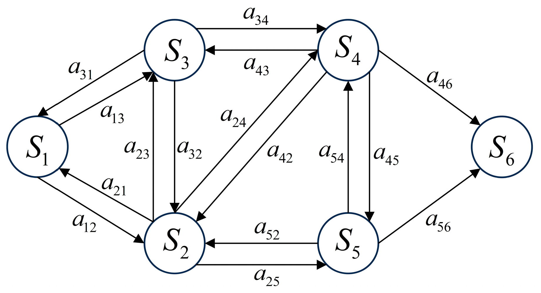
This paper established a radar state transition diagram using six operation modes of a MFR as states, as shown in Figure 12. The states S 1 S 6 represent the STT, MTT, TAS, TWS, RWS, and VS modes, with their threat levels defined as 10, 8, 6, 5, 3, and 1, respectively. The VS mode had the lowest threat level and was set as the radar’s target state. During training, the STT mode was set as the initial state. The rewards corresponding to the differences in threat levels of −4, −3, −2, −1, 1, 2, 3, and 4 were 20, 10, 5, 1, −1, −5, −10, and −20, respectively.
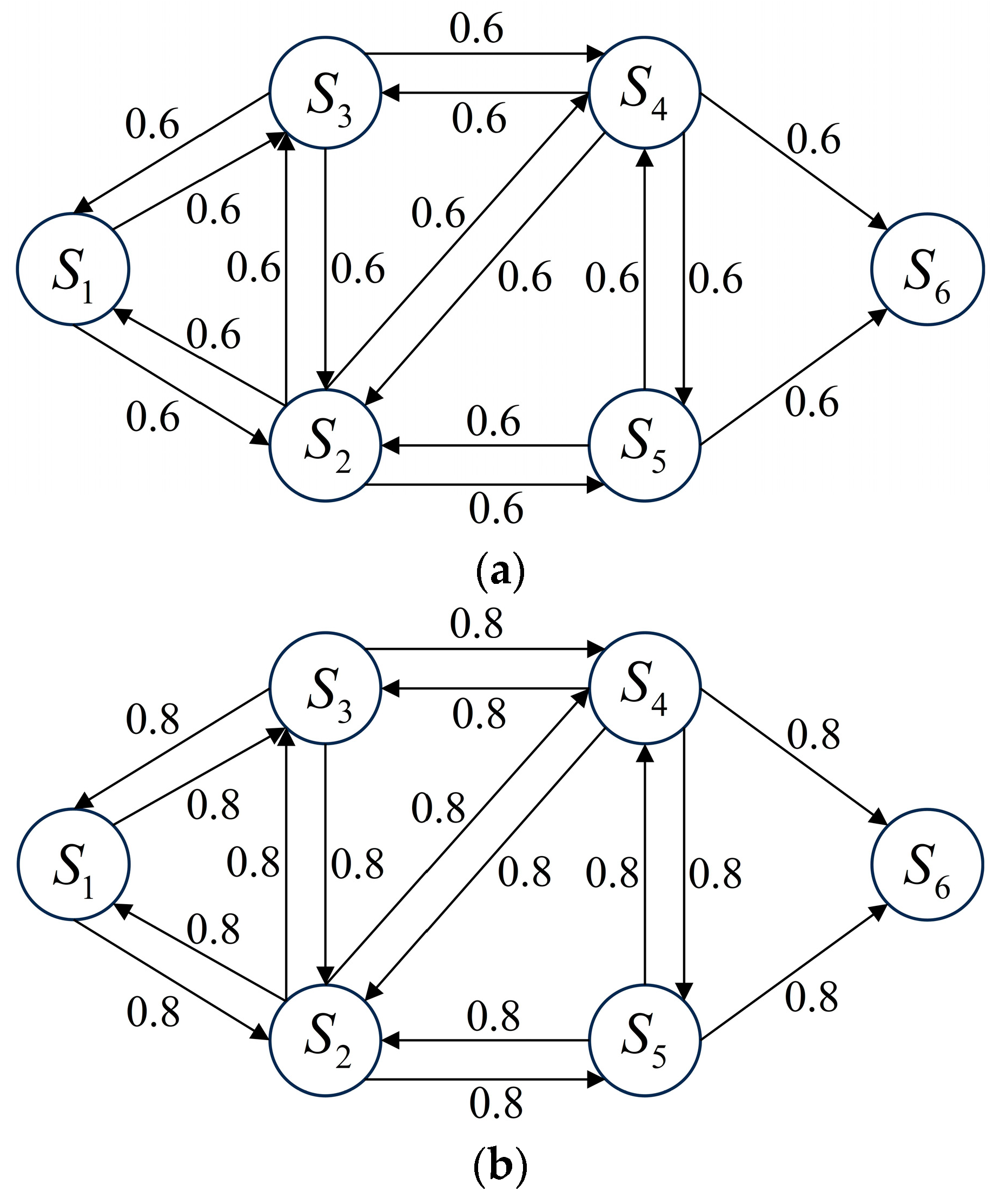
In the radar state transition diagram, a i j represents the jamming pattern that can transition the radar state from S i to S j , causing the radar state to change with probability p i j . To examine the effectiveness of the proposed algorithm across various environments, three different radar state transition models were defined: env_1, env_2, and env_3. We set the radar state transition probabilities in env_1, env_2, and env_3 to 0.6, 0.8, and 0.9, respectively, as shown in Figure 13. In env_1, the uncertainty of radar state transitions was the highest, making the environment the most unstable and posing the greatest challenge to the jammer.
The simulation experiments were conducted in a Python environment. The hardware resources included an AMD Ryzen 7 6800H processor with a clock speed of 3.2 GHz and 16 GB of memory, sourced from AMD Inc., Santa Clara, USA. Experimental parameter settings are shown in Table 1.
In reinforcement learning, the sum of Q-values can be used to evaluate whether the algorithm has converged. The algorithm is considered to have converged when the difference in the sum of Q-values between consecutive training episodes is less than a threshold. After each round of training, we computed the sum of all elements in the Q-table, defined as follows:
Q = i = 1 | S | j = 1 | A | q i j ,
where | S | represents the number of radar states, and | A | represents the number of jamming patterns. The Q-value sum curves of the Q-learning algorithm and the MTEQL algorithm in the three different environments are shown in Figure 14a–c.
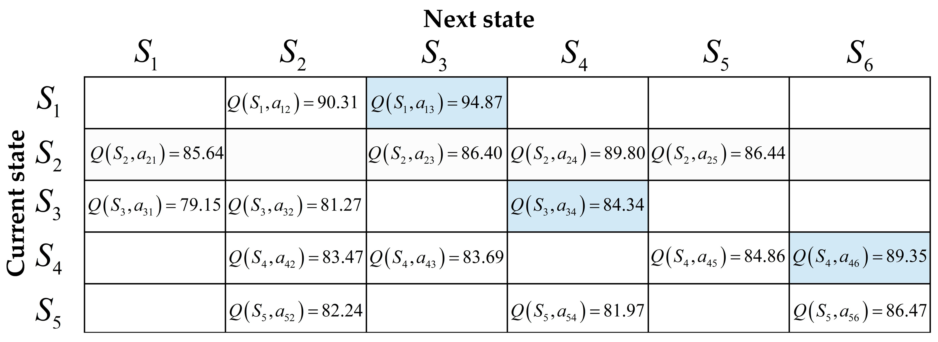
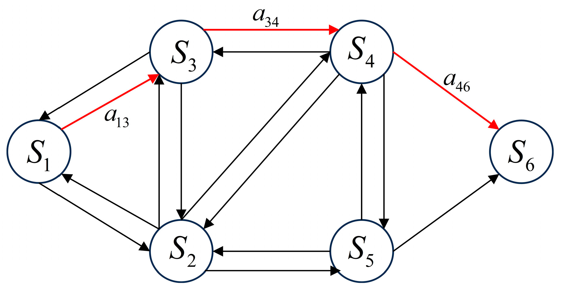
It can be observed that in all three environments, the MTEQL algorithm converged earlier than the Q-learning algorithm. The number of training iterations required for convergence in the three environments was 6100, 6400, and 7800, respectively, representing reductions of 28.23%, 20%, and 14.29% compared to the convergence iterations of the traditional Q-learning algorithm. Moreover, the more unstable the environment, the better the performance improvement in the MTEQL algorithm. Due to the parallel processing nature of MTEQL, each iteration may involve a greater computational load, which varies with the number of Markov environment sets. The computational load is equivalent to a constant multiple of that in the traditional Q-learning algorithm. However, the MTEQL method compensates for this by significantly reducing the number of iterations required for convergence. This results in a net decrease in convergence time, thereby improving the efficiency of jamming strategy generation. Taking environment env_1 as an example, the Q-table generated after convergence is shown in Figure 15. It can be seen that the optimal jamming patterns corresponding to the s 1 s 5 state were a 13 , a 24 , a 34 , a 46 , and a 56 . The optimal policy can be identified as S 1 a 13 S 3 a 34 S 4 a 46 S 6 , as shown in Figure 16. The red arrows represent the optimal jamming actions chosen by the jammer, demonstrating that the jammer transitioned the radar from the initial state to the target state in the fewest steps.
To investigate the impact of different numbers of Markov environments on algorithm performance, we varied the number of Markov environments by setting K to 2, 3, 4, and 5, respectively. Experiments were conducted in the env_1 environment, and the resulting Q-value sum curves are shown in Figure 17.
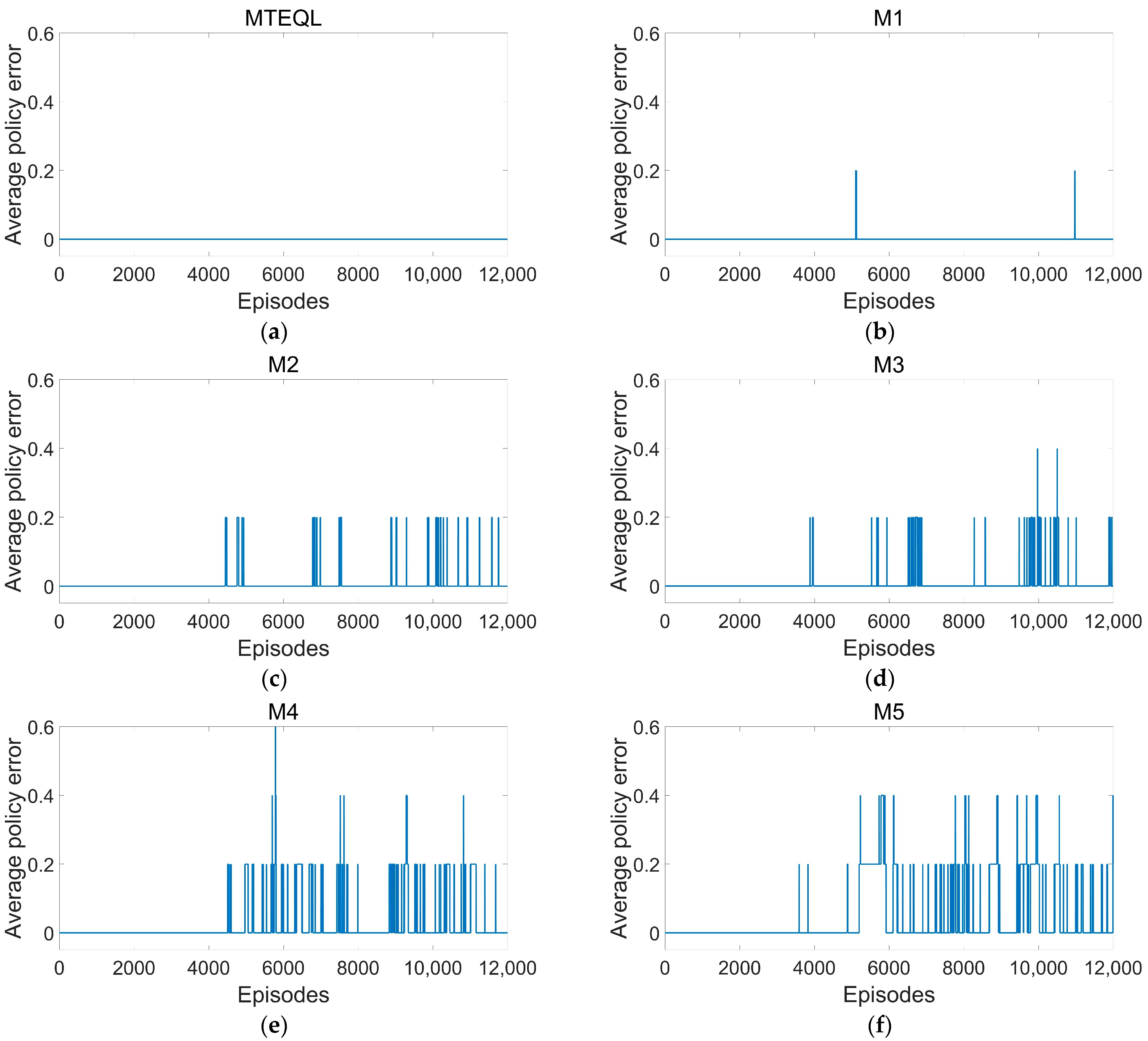
The experimental results indicated that the algorithm converged when K was set to 2, 3, 4, and 5. The Q-values represent the expected cumulative rewards for taking certain actions in given states. The faster convergence of MTEQL allowed it to stabilize and optimize its strategy more quickly, which is the primary advantage we highlighted here. However, the convergence speed was slightly faster when K was set to 5 compared to the other three cases. This is because, with K set to 5, the jammer can learn more knowledge from indirect experiences, enhancing its exploration capability in unknown environments. The accuracy of the policy determines whether the jammer can complete the jamming task, and the average policy error (APE) can measure the accuracy of the strategy. The APE is the probability that the jamming pattern chosen in each state is not the optimal jamming pattern out of all states. Its calculation formula is as follows:
A P E = 1 | S | s = 1 | S | 1 ( π ( s ) π ^ ( s ) ) ,
where π is the optimal policy calculated according to Equation (5), and π ^ is the policy learned from different Markov environments. Figure 18a shows the average strategy error obtained by the MTEQL algorithm, and Figure 18b–f shows the average strategy error for Markov environments M ( 1 ) to M ( 5 ) .
The experimental results indicated that the strategy derived using the MTEQL algorithm exhibited an APE of zero per round. In contrast, the strategy generated from the original Markov environment, M1, contained errors, suggesting that the traditional Q-learning algorithm may encounter decision errors during the training process. Furthermore, as the value of K increased, the APE of the training strategy also rose. These findings demonstrated that integrating strategies obtained from training multiple Markov environments is a feasible approach, yielding optimal strategies.

5. Conclusions

Reinforcement-learning-based jamming strategy generation methods can adjust jamming strategies in real time, understanding the patterns of radar operation modes in adversarial scenarios to find the optimal jamming strategy for each mode. However, traditional Q-learning algorithms face challenges, such as limited exploration capabilities in unknown environments and long convergence times. To address these issues and improve the jamming decision efficiency, enhance the jammer’s exploration capability in the strategy space, and reduce decision error rates, we introduced an efficient method for generating jamming strategies based on multi-timescale ensemble Q-learning. To confirm the algorithm’s effectiveness in real battlefield environments, we first constructed an adversarial scenario between the jammer and the radar and thoroughly analyzed the rules of radar operation mode transitions. Additionally, multiple Markov environments were utilized to accelerate the jammer’s understanding of the environment and speed up the algorithm’s convergence. Simulation experiments demonstrated that the proposed algorithm converged faster than the Q-learning algorithm in various environments and performed better in unstable environments. Moreover, the algorithm exhibited a very low average strategy error, capable of generating optimal jamming strategies.
Of course, the model established in this paper was relatively simple, considering only the impact of jamming on radar states and not accounting for factors such as targets. Therefore, the next step could be to improve the model to make it more representative of real-world adversarial scenarios. Additionally, the electromagnetic environment in actual battlefields is complex, and merely selecting the optimal jamming pattern may not effectively interfere with the radar. Optimizing jamming parameters based on the selected jamming pattern is also a direction for future research.

Author Contributions

Conceptualization, J.Q. and Q.Z.; methodology, J.Q. and Z.X.; software, J.Q. and Z.Y.; validation, J.Q., Z.L., and S.S.; formal analysis, J.Q.; investigation, J.Q. and Z.X.; resources, Z.L.; data curation, J.Q.; writing—original draft preparation, J.Q.; writing—review and editing, J.Q., Z.Y., S.S., and Q.X.; visualization, J.Q.; supervision, J.Q. and Z.L.; project administration, Q.Z.; funding acquisition, Q.Z. and Z.L. All authors have read and agreed to the published version of the manuscript.

Funding

This paper is partly supported by the National Natural Science Foundation of China under grant number 62301581, the China Postdoctoral Science Foundation under grant number 2023M734313 and the Postgraduate Scientific Research Innovation Project of Hunan Province under grant number CX20230045.

Data Availability Statement

The data are available to readers by contacting the corresponding author.

Acknowledgments

The authors would like to thank all of the reviewers and editors for their comments on this paper.

Conflicts of Interest

The authors declare no conflicts of interest.

References

  1. Zhou, Y.; An, W.; Guo, F.; Liu, Z.; Jiang, W. Principles and Technologies of Electronic Warfare System; Publishing House of Electronics Industry: Beijing, China, 2014. [Google Scholar]
  2. Huang, Z.; Wang, X.; Zhao, Y. Overview of cognitive electronic warfare. J. Natl. Univ. Def. Technol. 2023, 45, 1–11. [Google Scholar]
  3. Charlish, A. Autonomous Agents for Multi-Function Radar Resource Management. Ph.D. Thesis, University College London, London, UK, 2011. [Google Scholar]
  4. Apfeld, S.; Charlish, A.; Ascheid, G. Modelling, learning and prediction of complex radar emitter behaviour. In Proceedings of the 2019 18th IEEE International Conference on Machine Learning and Applications (ICMLA), Boca Raton, FL, USA, 16–19 December 2019; pp. 305–310. [Google Scholar]
  5. Liu, D.; Zhao, Y.; Cai, X.; Xu, B.; Qiu, T. Adaptive scheduling algorithm based on cpi and impact of tasks for multifunction radar. IEEE Sens. J. 2019, 19, 11205–11212. [Google Scholar] [CrossRef]
  6. Han, C.; Kai, L.; Zhou, Z.; Zhao, Y.; Yan, H.; Tian, K.; Tang, B. Syntactic modeling and neural based parsing for multifunction radar signal interpretation. IEEE Trans. Aerosp. Electron. Syst. 2024, 60, 5060–5072. [Google Scholar]
  7. Wang, S.; Zhu, M.; Li, Y.; Yang, J.; Li, Y. Recognition, inference, and prediction of advanced Multi-Function radar systems behaviors: Overview and prospects. J. Signal Process. 2024, 40, 17–55. [Google Scholar]
  8. Johnston, S.L. Radar Electronic Counter-Countermeasures. IEEE Trans. Aerosp. Electron. Syst. 1978, AES14, 109–117. [Google Scholar] [CrossRef]
  9. Wang, S.; Bao, Y.; Li, Y. The architecture and technology of cognitive electronic warfare. Sci. Sin. Inform. 2018, 48, 1603–1613. [Google Scholar] [CrossRef]
  10. Dahle, R. EW 104: Electronic Warfare Against a New Generation of Threats. Microw. J. 2024, 67, 118. [Google Scholar]
  11. Haykin, S. Cognitive radar: A way of the future. IEEE Signal Process. Mag. 2006, 23, 30–40. [Google Scholar] [CrossRef]
  12. Sudha, Y.; Sarasvathi, V. A Model-Free Cognitive Anti-Jamming Strategy Using Adversarial Learning Algorithm. Cybern. Inf. Technol. 2022, 22, 56–72. [Google Scholar] [CrossRef]
  13. Darpa, A. Behavioral Learning for Adaptive Electronic Warfare. In Darpa-BAA-10-79; Defense Advanced Research Projects Agency: Arlington, TX, USA, 2010. [Google Scholar]
  14. Knowles, J. Regaining the advantage—Cognitive electronic warfare. J. Electron. Def. 2016, 39, 56–62. [Google Scholar]
  15. Zhou, H. An introduction of cognitive electronic warfare system. In Proceedings of the International Conferences on Communications, Signal Processing, and Systems, Dalian, China, 14–16 July 2018. [Google Scholar]
  16. So, R.P.; Ilku, N.; Sanguk, N. Modeling and simulation for the investigation of radar responses to electronic attacks in electronic warfare environments. Secur. Commun. Netw. 2018, 2018, 3580536. [Google Scholar]
  17. Purabi, S.; Kandarpa, K.S.; Nikos, E.M. Artificial Intelligence Aided Electronic Warfare Systems- Recent Trends and Evolving Applications. IEEE Access 2020, 8, 224761–224780. [Google Scholar]
  18. Nepryaev, A.A. Cognitive radar control system using machine learning. In IOP Conference Series: Materials Science and Engineering; IOP Publishing: Bristol, UK, 2021; Volume 1047, p. 012119. [Google Scholar]
  19. BIS Research. Cognitive electronic warfare: An artificial intelligence approach. Microw. J. 2021, 64, 110. [Google Scholar]
  20. du Plessis, W.P.; Osner, N.R. Cognitive electronic warfare (EW) systems as a training aid. In Proceedings of the Electronic Warfare International Conference (EWCI), Bangalore, India, 13–16 February 2018; pp. 1–7. [Google Scholar]
  21. Xiao, L.; Liu, D. Modeling method of combat mission based on OODA loop. MATEC Web Conf. 2022, 355, 02015. [Google Scholar]
  22. Zhang, B.; Zhu, W. Overview of jamming decision-making method for Multi-Function phased array radar. J. Ordnance Equip. Eng. 2019, 40, 178–183. [Google Scholar]
  23. Zhang, C.; Wang, L.; Jiang, R.; Hu, J.; Xu, S. Radar jamming decision-making in cognitive electronic warfare: A review. IEEE Sens. J. 2023, 23, 11383–11403. [Google Scholar] [CrossRef]
  24. Liangliang, G.; Shilong, W.; Tao, L. A radar emitter identification method based on pulse match template sequence. In Proceedings of the 2010 2nd International Conference on Signal Processing Systems, Dalian, China, 5–7 July 2010. [Google Scholar]
  25. Li, K.; Jiu, B.; Liu, H. Game theoretic strategies design for monostatic radar and jammer based on mutual information. IEEE Access 2019, 7, 72257–72266. [Google Scholar] [CrossRef]
  26. Bachmann, D.J.; Evans, R.J.; Moran, B. Game theoretic analysis of adaptive radar jamming. IEEE Trans. Aerosp. Electron. Syst. 2011, 47, 1081–1100. [Google Scholar] [CrossRef]
  27. Sun, H.; Tong, N.; Sun, F. Jamming design selection based on D-S Theory. J. Proj. Rocket. Missiles Guid. 2003, 202, 218–220. [Google Scholar]
  28. Sutton, R.S.; Barto, A.G. Reinforcement learning: An introduction. Neural Netw. IEEE Trans. 1998, 19, 1054. [Google Scholar] [CrossRef]
  29. Rummery, G.A.; Niranjan, M. On-line q-learning using connectionist systems. Tech. Rep. 1994, 37, 335–360. [Google Scholar]
  30. Sutton, R.S. Learning to predict by the methods of temporal differences. Mach. Learn. 1988, 3, 9–44. [Google Scholar] [CrossRef]
  31. Watkins, C.; Dayan, P. Q-learning. Mach. Learn. 1992, 8, 279–292. [Google Scholar] [CrossRef]
  32. Ribeiro, R.; Koerich, A.L.; Enembreck, F. Noise tolerance in reinforcement learning algorithms. In Proceedings of the 2007 IEEE/WIC/ACM International Conference on Intelligent Agent Technology (IAT’07), Fremont, CA, USA, 2–5 November 2007. [Google Scholar]
  33. Llorente, F.; Martino, L.; Read, J.; Delgado-Gómez, D. A survey of Monte Carlo methods for noisy and costly densities with application to reinforcement learning and ABC. Int. Stat. Rev. 2024, 1. [Google Scholar] [CrossRef]
  34. Liu, W.; Xiang, S.; Zhang, T.; Han, Y.; Guo, X.; Zhang, Y.; Hao, Y. Judgmentally adjusted Q-values based on Q-ensemble for offline reinforcement learning. Neural Comput. Appl. 2024, 36, 15255–15277. [Google Scholar] [CrossRef]
  35. Li, Y.; Zhu, Y.; Gao, M. Design of cognitive radar jamming based on Q-Learning Algorithm. Trans. Beijing Inst. Technol. 2015, 35, 1194–1199. [Google Scholar]
  36. Zhang, B.; Zhu, W. Construction and key technologies of cognitive jamming decision-making system against MFR. Syst. Eng. Electron. 2020, 42, 1969–1975. [Google Scholar]
  37. Zhu, B.; Zhu, W.; Li, W.; Yang, Y.; Gao, T. Research on decision-making modeling of cognitive jamming for multi-functional radar based on Markov. Syst. Eng. Electron. 2022, 44, 2488–2497. [Google Scholar]
  38. Zhu, B.; Zhu, W.; Li, W.; Li, J.; Yang, Y. Multi-function radar jamming decision method based on planning steps adaptive Dyna-Q. Ordnance Ind. Autom. 2022, 41, 52–58. [Google Scholar]
  39. Li, H.; Li, Y.; He, C.; Zhan, J.; Zhang, H. Cognitive electronic jamming decision-making method based on improved Q-learning algorithm. Int. J. Aerosp. Eng. 2021, 2021, 8647386. [Google Scholar] [CrossRef]
  40. Zhang, C.; Song, Y.; Jiang, R.; Hu, J.; Xu, S. A cognitive electronic jamming decision-making method based on q-learning and ant colony fusion algorithm. Remote Sens. 2023, 15, 3108. [Google Scholar] [CrossRef]
  41. Zheng, S.; Zhang, C.; Hu, J.; Xu, S. Radar-jamming decision-making based on improved q-learning and fpga hardware implementation. Remote Sens. 2024, 16, 1190. [Google Scholar] [CrossRef]
  42. Zhang, B.; Zhu, W. DQN based decision-making method of cognitive jamming against multifunctional radar. Syst. Eng. Electron. 2020, 42, 819–825. [Google Scholar]
  43. Zou, W.; Niu, C.; Liu, W.; Gao, O.; Zhang, H. Cognitive jamming decision-making method against multifunctional radar based on A3C. Syst. Eng. Electron. 2023, 45, 86–92. [Google Scholar]
  44. Feng, L.W.; Liu, S.T.; Xu, H.Z. Multifunctional radar cognitive jamming decision based on dueling double deep q-network. IEEE Access 2022, 99, 112150–112157. [Google Scholar] [CrossRef]
  45. Zhang, Y.; Huo, W.; Huang, Y.; Zhang, C.; Pei, J.; Zhang, Y.; Yang, J. Jamming policy generation via heuristic programming reinforcement learning. IEEE Trans. Aerosp. Electron. Syst. 2023, 59, 8782–8799. [Google Scholar] [CrossRef]
  46. Mao, S. Research on Intelligent Jamming Decision-Making Methods Based on Reinforcement Learning. Master’s Thesis, Harbin Institute of Technology, Harbin, China, 2021. [Google Scholar]
  47. Zhang, P.; Ding, H.; Zhang, Y.; Li, B.; Huang, F.; Jin, Z. Multi-agent autonomous electronic jamming system based on information sharing. J. Zhejiang Univ. Eng. Sci. 2022, 56, 75–83. [Google Scholar]
  48. Pan, Z.; Li, Y.; Wang, S.; Li, Y. Joint optimization of jamming type selection and power control for countering multi-function radar based on deep reinforcement learning. IEEE Trans. Aerosp. Electron. Syst. 2023, 59, 108965. [Google Scholar] [CrossRef]
  49. Zhang, W.; Zhao, T.; Zhao, Z.; Ma, D.; Liu, F. Performance analysis of deep reinforcement learning-based intelligent cooperative jamming method confronting multi-functional networked radar. Signal Process. 2023, 207, 108965. [Google Scholar] [CrossRef]
  50. Kirkpatrick, S.; Gelatt, C.D.; Vecchi, M.P. Optimization by simulated annealing. Science 1983, 220, 671–680. [Google Scholar] [CrossRef]
  51. Metropolis, N.; Rosenbluth, A.W.; Rosenbluth, M.N.; Teller, A.H.; Teller, E. Equation of state calculations by fast computing machines. J. Chem. Phys. 1953, 21, 1087–1092. [Google Scholar] [CrossRef]
  52. Hastings, W.K. Monte Carlo sampling methods using Markov chains and their applications. Biometrika 1970, 57, 97–109. [Google Scholar] [CrossRef]
  53. Bozkus, T.; Mitra, U. Multi-timescale ensemble Q-learning for markov decision process policy optimization. IEEE Trans. Signal Process. 2024, 72, 1427–1442. [Google Scholar] [CrossRef]
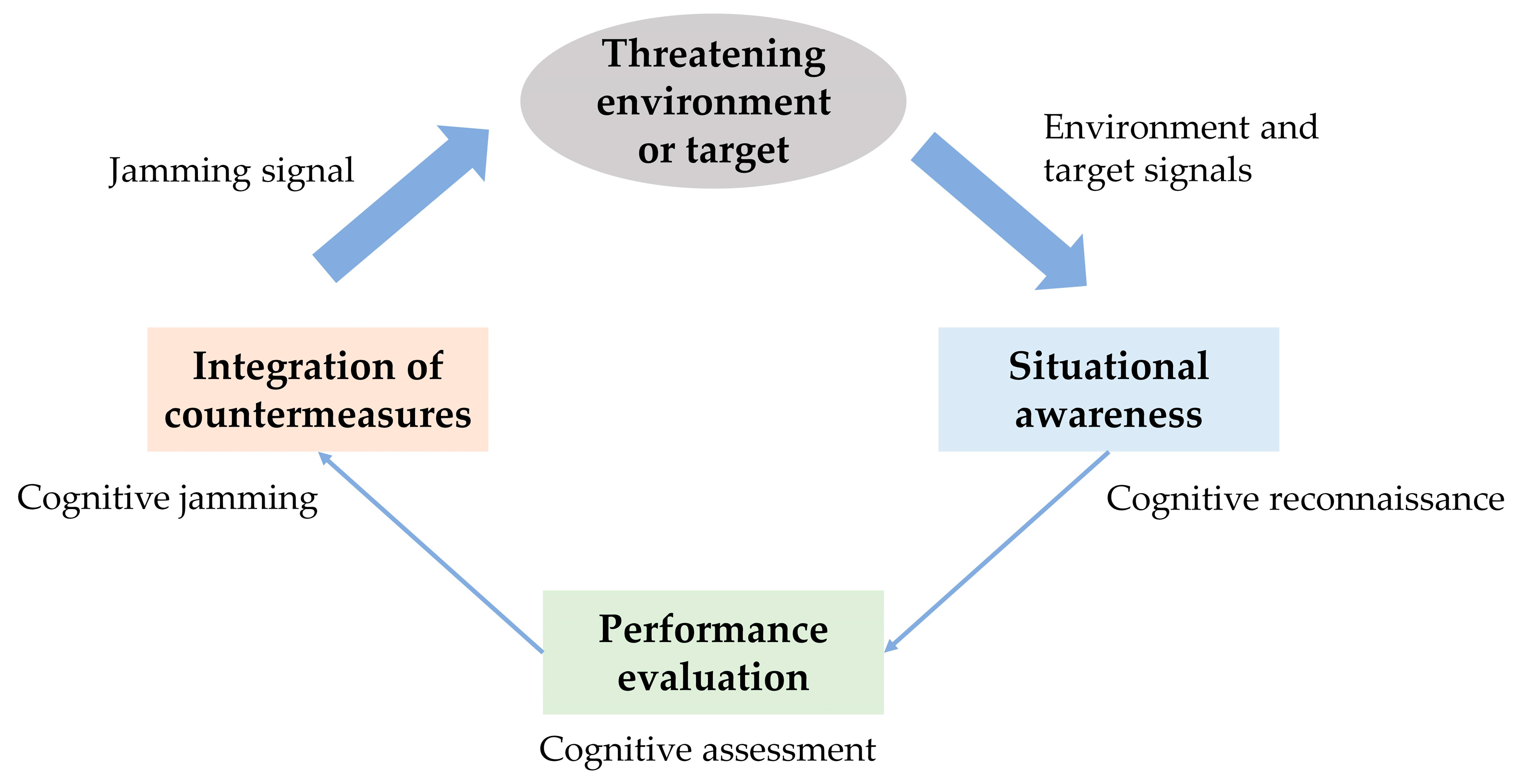
Figure 1. Closed-loop cognitive radar countermeasure process, integrating reconnaissance, evaluation, and jamming phases.
Remotesensing 16 03158 g001
Figure 2. Prior knowledge influences accurate jamming decisions by shaping templates, profit matrices, and event probability calculations.
Remotesensing 16 03158 g002
Figure 3. Radar countermeasure scenario diagram.
Remotesensing 16 03158 g003
Figure 4. Switching rule of the MFR’s operation modes in the absence of jamming.
Remotesensing 16 03158 g004
Figure 5. Switching rule of the MFR’s operation modes.
Remotesensing 16 03158 g005
Figure 6. Jamming effect evaluation.
Remotesensing 16 03158 g006
Figure 7. Jamming strategy generation algorithm table based on Q-learning.
Remotesensing 16 03158 g007
Figure 8. The overall block diagram of the jamming strategy generation algorithm based on MTEQL.
Remotesensing 16 03158 g008
Figure 9. Original and synthetic Markov environments.
Remotesensing 16 03158 g009
Figure 10. Q-learning algorithm and MTEQL algorithm.
Remotesensing 16 03158 g010
Figure 11. Jamming strategy generation algorithm table based on MTEQL.
Remotesensing 16 03158 g011
Figure 12. Radar state transition diagram.
Remotesensing 16 03158 g012
Figure 13. Radar state transition diagram under different environments: (a) env_1, (b) env_2, and (c) env_3.
Remotesensing 16 03158 g013aRemotesensing 16 03158 g013b
Figure 14. The sum of Q-values under different circumstances: (a) env_1, (b) env_2, and (c) env_3.
Remotesensing 16 03158 g014
Figure 15. Q-table after convergence. The blue box indicates the Q-values of the optimal jamming pattern for the current state.
Remotesensing 16 03158 g015
Figure 16. Optimal jamming strategy. The red arrows indicate the selected optimal jamming strategy.
Remotesensing 16 03158 g016
Figure 17. The sum of Q-values in different numbers of Markov environments.
Remotesensing 16 03158 g017
Figure 18. Average policy errors in different Markov environments: (a) MTEQL, (b) M1, (c) M2, (d) M3, (e) M4, and (f) M5.
Remotesensing 16 03158 g018
Table 1. Simulation parameter settings.
ParametersValue
Sampling path length, l 200
Minimum number of times for each state transition pair, v 40
Training episodes, E n u m 12,000
The total number of Markov environments, K 5
Learning rate, α 0.1
Discount factor, γ 0.9
Replacement rate, u t 0.5
Disclaimer/Publisher’s Note: The statements, opinions and data contained in all publications are solely those of the individual author(s) and contributor(s) and not of MDPI and/or the editor(s). MDPI and/or the editor(s) disclaim responsibility for any injury to people or property resulting from any ideas, methods, instructions or products referred to in the content.