Article

Hyperspectral Data Can Differentiate Species and Cultivars of C3 and C4 Turf Despite Measurable Diurnal Variation

by
Thomas A. Cushnahan
1,2,
Miles C. E. Grafton
1,
Diane Pearson
1 and
Thiagarajah Ramilan
1,*
1
School of Agriculture and Environment, College of Sciences, Massey University, Palmerston North 4442, New Zealand
2
AgResearch Ltd., Grasslands Research Centre, Private Bag 11008, Palmerston North 4410, New Zealand
*
Author to whom correspondence should be addressed.
Remote Sens. 2024, 16(17), 3142; https://doi.org/10.3390/rs16173142
Submission received: 7 July 2024 / Revised: 16 August 2024 / Accepted: 20 August 2024 / Published: 26 August 2024
(This article belongs to the Section Remote Sensing in Agriculture and Vegetation)

Abstract

:
The ability to differentiate species is not adequate for modern forage breeding programs. The measurement of persistence is currently a bottleneck in the breeding system that limits the throughput of cultivars to the marketplace and prevents it from being selected as a trait. The use of hyperspectral data obtained through remote sensing offers the potential to reduce guesswork by identifying the distribution of pasture species, but only if such data alone can distinguish the subtle differences within species, i.e., cultivars. The implementation of this technology faces many challenges due to the spectral and temporal variability of species. To understand the spectral variability between and within species groups, differentiation using hyperspectral data from monoculture plots of turf species was utilized. Spectral data were collected over a year using an ASD FieldSpec® and canopy pasture probe (CAPP). The plots consisted of monocultures of various species, and cultivars (a total of 10 plots). Linear discriminant analysis (LDA) was conducted on the full spectrum and reduced band data. This technique successfully differentiated the species with high accuracy (>98%). We demonstrate the potential of hyperspectral data and analysis techniques to accurately separate differences down to cultivar level. We also show that diurnal variation is measurable in the spectra but does not preclude differentiation.

1. Introduction

This article explores the use of hyperspectral sensing in a controlled field setting to better understand the capabilities and limitations of the technology to separate varieties and cultivars of both C3 and C4 fine turf species and cultivars of the same species. The physiological differences that allow plants to be classified create variation in reflectance, so we hypothesized it would be possible to differentiate species and even cultivars of species only using hyperspectral data. Turf species were used as a surrogate for agricultural pasture species as they were available in a diverse array of species and cultivars.
In attempting to understand the spectral reflectance of pasture species, this research acknowledges that grass and forage breeders experience problems assessing the long-term benefits of sown species. Persistence in the managed pasture environment is the ability of a sown species to compete with self-seeded species and remain within the sward after sowing. A number of metrics have been suggested to measure persistence in the sown sward, but all rely on visual assessment by experienced personnel [1]. The reliance on operator dependent pattern recognition leaves the task subject to intra- and inter-observer variability, which is typically mitigated by using multiple experts [2]. The need for multiple experts and the time needed to assess the trials also create logistical issues in finding, coordinating, and paying for the required number of experts to be on site at the same time. This limits the throughput of such trials, as some prospects must be excluded earlier in the breeding process. There is a probability that the cumulative benefits (yield) from more persistent species might outperform less persistent species that are otherwise superior. Varieties that might have greater persistence could therefore be excluded, resulting in breeders not readily selecting for this trait. Hyperspectral remote sensing could enable a data-driven selection process that requires less expert time and simultaneously increases throughput, but there are potential obstacles to this goal.
It is common that field hyperspectral surveys take the time of day for sample collection into consideration to ensure repeatable results. This is particularly true if the sample collection relies on illumination from the sun, as the deleterious effects of sun angle are well established [3,4,5,6,7,8]. Other important plant characteristics that change throughout the day, including carbohydrate [9] and photosynthetic function [10], also need to be considered. How the diurnal changes in plant characteristics impact species identification via spectral reflectance is not well known. This work investigates the extent of diurnal change in plant spectral signatures and whether those variations are sufficient to interfere with species differentiation.
Differentiation is an important step prior to the challenges in species identification. Differentiation and identification are not the same. Differentiation is defined here as the ability to predict the correct target from a small, confined, and defined group. This can be thought of as a multiple-choice type of question where a probability exists of choosing the correct answer in error. Identification is the ability to identify a target in any context with an unlimited list of options. The structural and chemical variability within and between species has a large impact on the signal returned from reflectance and thus on our ability to differentiate them. Plant species and communities are physiologically adapted to specific environments, which enables each to compete in those unique circumstances [11]. These adaptations to environmental forces can enhance or obstruct differentiation. When different species are adapted to the same environmental niche (evolutionary convergence) [12], they may exhibit similarities in their spectral returns and create difficulties when trying to distinguish them [13]. The adaptations may also create distinctiveness that can be leveraged for identification as found by Wang, Hunt [14]. Researchers employ some remote sensing and precision agriculture techniques in breeding and cultivar development [15,16,17,18], but not yet for cultivar differentiation, perhaps because the breeding lines are so closely related. This study builds on the work that has been started by others to solve these problems.
Caturegli, Lulli [19] examined a series of spectral indices and associated traits of twenty turf subjects to help understand if they could be distinguished from satellite data with mixed results. They found that, although helpful to highlight spectral differences, indices were not capable of separating within species variation. Irisarri, Oesterheld [20] also investigated the reflectance of seven C3 and C4 turf species. Their work focused on plants in pots and used hyperspectral data ranging from 350 to 1075 nm. Other research on turf focused on the nutrient status [21,22] and water status [23,24,25] of turf species. Some studies, e.g., Schmidt and Skidmore [26] and others, have sought to map species richness or diversity in grasslands [27,28]. Many of the attempts to differentiate grass species have focused on the separation of C3 and C4 species. In doing so, most have taken advantage of the spectral variability that they exhibit at different times of the year [14,29]. Although this is a step forward in our understanding, the reality is that such a method requires data from two seasons to carry out. Liu and Cheng [30] have shown that it is possible to differentiate C3 from C4 plant functional types within a single data collection. However, the challenge still exists to define different pasture species or cultivars within those C3 and C4 groups. For the technology to be of practical use, it must differentiate varieties and cultivars from a single data collection without the need for additional supplementary data.
The question we sought to answer with this work was whether the spectral similarity of species or cultivars and the spectral differences caused by diurnal variation would work together to suppress our ability to differentiate them. The aim of the study is to assess if hyperspectral data can be used to differentiate species in an established, field-based, pastoral setting. The objectives were to identify and define the extent of species or cultivar differentiation and to assess if subjects can be separated with the technology alone, without supplementary information.

2. Materials and Methods

The trial sites were located on the north island of New Zealand, 6 km south of the Palmerston North CBD, at the New Zealand Sports Turf Institute (NZSTI). The location was selected for its wide range of C3 and C4 turfgrass species and some broad-leafed species grown in homogenous, long-term trial plots. The sites were established for various research trials and as teaching aids for greenkeeper training.

2.1. Site Description

For simplicity and to avoid misnomers, the various species and cultivars used in the trial are referred to as subjects. Managed monoculture sites of turfgrass and broadleaf turf species were used to reduce external variability. Sites varied in size from 2 m2 to 12 m2 (averaging around 10 m2) and were positioned within a single 50 m area on a series of terraces. The sites had been growing for at least two years, so they were well established and mature. The species used in the trial are listed in Table 1.
It was assumed that it would be more difficult to distinguish plants with close taxonomic associations, such as the closely related, elite-performing ryegrass accessions studied in forage trials. The subjects were selected for their purity and to represent a wide range of taxonomies, i.e., family, genus, species, variety, and cultivar, as illustrated in Figure 1 and in line with other work [19,31]. The wide taxonomic range of subjects was hypothesized to offer better insight into the technology’s threshold for differentiation.
Cotula (Leptinella sp.) was the only dicotyledon subject in the trial, it is the primary species used on New Zealand bowling greens and was maintained at 5 mm. All other subjects were monocotyledons from the poaceae genera but can again be further distinguished. The couch and Kikuyu are both C4 plants; that is, they have physiological adaptations to both their leaf cell structure and cell metabolites [32] that differ from the remaining seven subjects. The remaining subjects are from the Agrostis, Festuca, and Lolium genera, with each having quite distinctive morphological differences. Lolium is from the same genera as the elite forage accessions bred for animal feed. The group has tufted growth habits, glossy, hairless leaves, and often a pink/purple tinge to the leaf base. Fescues have narrow, needle-like leaves, which reduces the surface area, an adaptation that provides tolerance to dry conditions. Agrostis have wider leaves; they produce both stolons and rhizomes, which form a dense spreading sward. They do well in many habitats, especially in damp soil conditions.

2.2. Reflectance Data Collection

Reflectance data from the sites was collected using an ASD FieldSpec® 4 High Resolution (Malvern Panalytical Ltd., Malvern, UK) with an attached CAPP [33]. The ASD collected reflectance in the visible near-infrared (VNIR) 350–1000 nm and shortwave infrared (SWIR) 1000–2500 nm to produce a combined reflectance curve from 350 nm to 2500 nm. The CAPP diameter on the ground is 32 cm, with elliptical internal sampling dimensions of 19.7 cm and 18.7 cm for the major and minor axes [34].

2.3. Collection of Data for Diurnal Analysis

Reflectance spectra were collected from all plots at 08.00, 10.00, 12.00, 14.00, and 16.00 h on the 3rd and 5th of September 2014 (Southern Hemisphere Spring). Sample areas were marked with location pegs (Figure 2) that remained in place for three days to ensure the collection of data from the same area on each occasion. The CAPP was rotated for each sample to account for variations in leaf orientation while maintaining positional accuracy at the same location. Data collection took place under bright and sunny conditions. Although sunny conditions were not needed for data collection (the CAPP had internal illumination), it did mean maximizing photosynthetic activity. Data collection took place three days after mowing to minimize the influence of mechanical damage.

2.4. Continued Data Collection for Subject Differentiation

Following the initial daily collection, spectral data were collected from each site every 4 to 6 weeks (weather-dependent) over the course of one year. Again, the internal illumination of the CAPP meant consistency in spectral data regardless of external illumination. Data were collected from various points within the core of the plots to optimize sample purity. Unfortunately, the Cynodon site was removed for operational reasons by the NZSTI towards the end of the trial period, while data collection for the other sites continued throughout the year.

2.5. Data Handling

All spectra from both datasets were corrected for variations in the internal sensors according to manufacturer specifications using the ViewSpec Pro software, v 6.20, (Malvern Panalytical Ltd., Malvern, UK) that is packaged with the ASD spectrometer. The corrected data were exported to Matlab® 8.4 and R 3.2.2 statistical software packages via Excel. The first and last fifty bands (350–400 nm and 2450–2500 nm) were excised due to signal-to-noise problems [35], resulting in each dataset having 2050 bands ranging from 400 nm to 2450 nm.

2.6. Statistics and Analysis

2.6.1. Pre-Processing

Preprocessing of spectral data is often necessary to simplify the relationships between spectra and target traits, and to maximize model performance [36].
The raw spectral data were transformed in two ways: by Standard Normal Variate (SNV) transformation ((x)−Mean(x)/Std(x)) [37] and by conversion to 1st derivative. The SNV is a widely used method to reduce the variability caused by the impact of nonspecific surface radiation scatter, differences in spectral pathlength, and chemical composition. [37]. For SNV calculation. the reflectance at a given wavelength has the average intensity for all wavelengths subtracted from it. The result is then divided by the standard deviation for all wavelengths to provide a corrected value for each.
Derivatives have a long history of use in the pre-processing of spectral data and with good reason, as they often improve performance [38,39]. The first derivative was calculated by applying the gap-segment algorithm, which included smoothing with a Savitzky–Golay filter. Smoothing is an important part of the derivative procedure as it is susceptible to noise [40]. The filter with a window size of 11, followed by a gap segment derivative with a segment size of 10, was carried out using the ‘prospectr’ package in ‘R’ [41].

2.6.2. Band Ranking and Band Reduction, U-Test

A Mann–Whitney U test (U-Test) was carried out in Matlab® to identify bands that were sensitive to species discrimination. The U-Test compared median values at each wavelength across all subjects to assess between-subject variation. Bands were ranked based on the cumulative results, with higher results considered more useful in classification or prediction.

2.6.3. Subject Differentiation with Linear Discriminate Analysis (LDA)

LDA is a statistical technique based on Fisher’s linear discriminant that is used for classification and pattern recognition. It tries to maintain the between-class variance by projecting a line that is orthogonal to the overall class variance to best separate the classes [42]. The LDA decision boundary is determined by both the position of the class centroid and the class distribution covariance [43]. The approach is applicable to numerical data, such as reflectance data, and is a good approach for classification [44]. LDA is used for a wide variety of classification problems, including facial analysis [45], complex pattern recognition [46], and the analysis of spectroscopic data [47,48]. The long history of its use and wide array of applications mean it is an easily accessible method for classification.
The LDA for the discrimination of subjects was first carried out using a small selection of the most prominent bands as predicted by the U test. The number of bands used was incrementally increased, and the accuracies were plotted to identify the optimal number for the highest accuracy. This approach was repeated for both standardized and derivative data.

2.6.4. Stepwise LDA

Stepwise feature selection was utilized to include or exclude features based on improvements in model performance. LDA with stepwise feature selection was employed to overcome the sensitivity of LDA to the Hughes effect [49,50]. The model was created and refined using a 10-fold repeated cross-validation approach with the ‘KLAR’ package in ‘R’ [51]. A reduced number of variables were identified for the analysis of collection time. The model was then independently validated on a previously isolated test dataset.
The LDA for diurnal collection time was carried out with the model built from a 30/70 (training/test) data split instead of the more common 80/20 data split. The decision was taken to use a 30/70 (training/test) split as it hindered the output somewhat and was more revealing of the limits of the analysis.

3. Results

3.1. Datasets

2800 total sample spectra (280 per subject) were collected in a series of collection events over one year, resulting in two primary datasets:
  • Diurnal dataset: This dataset (n = 2000) was examined for fluctuations in diurnal reflectance for each subject. Forty spectral samples per subject, at each of the five time periods, were collected over two days. Each spectral sample represents the average of ten automatically collected and averaged readings.
  • Differentiation dataset: The total dataset (n = 2800) collated data from all subjects over the 12 months, including the data used for diurnal analysis, to investigate subject separability and explore dimensionality reduction through band selection.
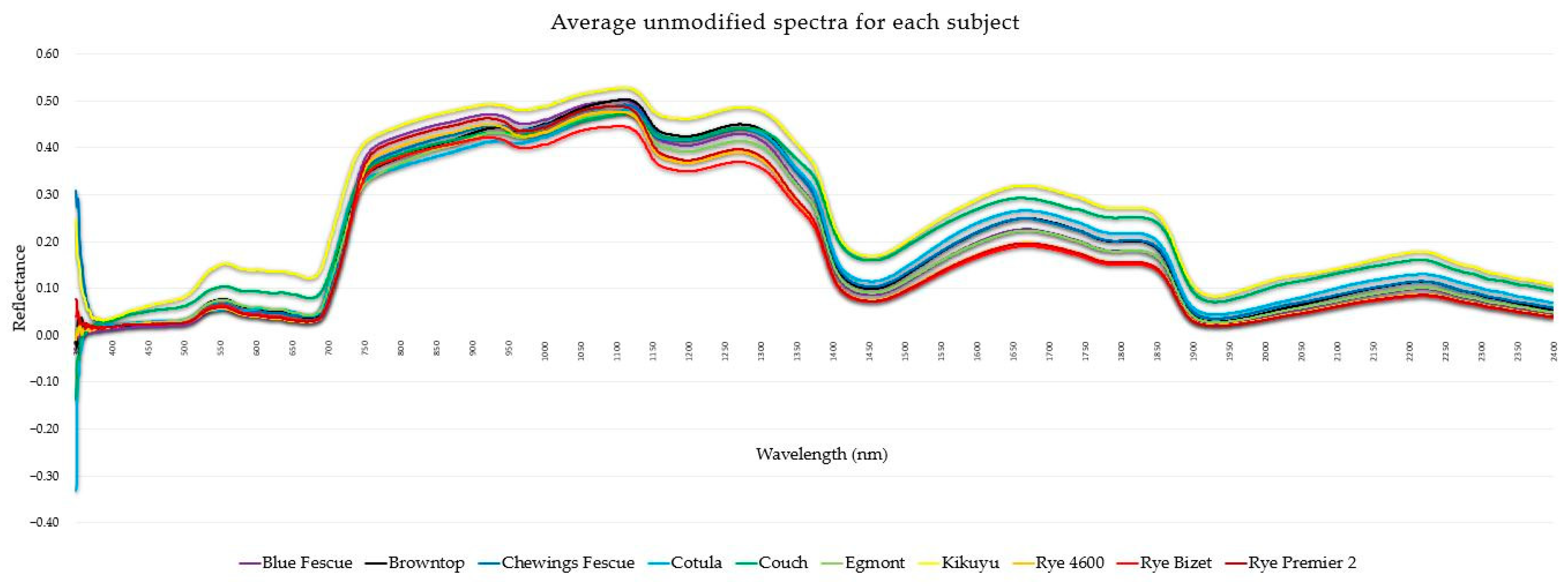
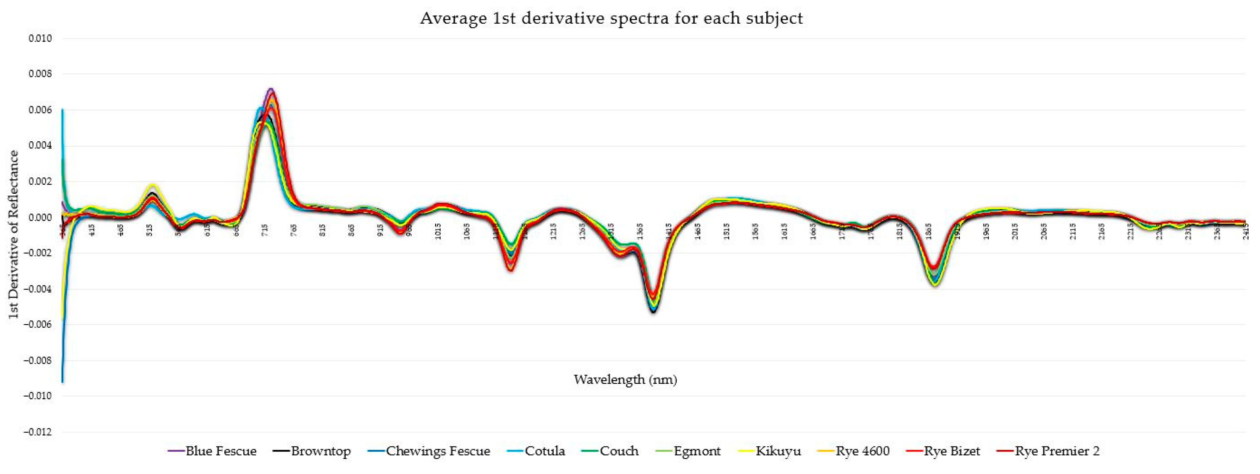
The subtle variations in reflectance recovered from each of the subjects are illustrated in Figure 3 and Figure 4, showing the overall similarity typical of vegetation reflectance.

3.2. Subject Differentiation with LDA

Both data transformations allowed the LDA to differentiate subjects. Table 2 and Table 3 show the output statistics from the LDA for the smallest number of bands used in the analysis. Both had relatively high overall accuracies >78%, with a general trend in the incorrect predictions made between the three Ryegrass cultivars and two fescues.
The optimum number of bands necessary for species differentiation varied with the pre-processing method (as seen in Table 4 and Table 5). Although both datasets ended up with similar prediction accuracy maxima, the 1st derivative data did so with fewer bands. Prediction accuracies of greater than 95% were achieved with as few as 50 bands.

3.3. Band Reduction

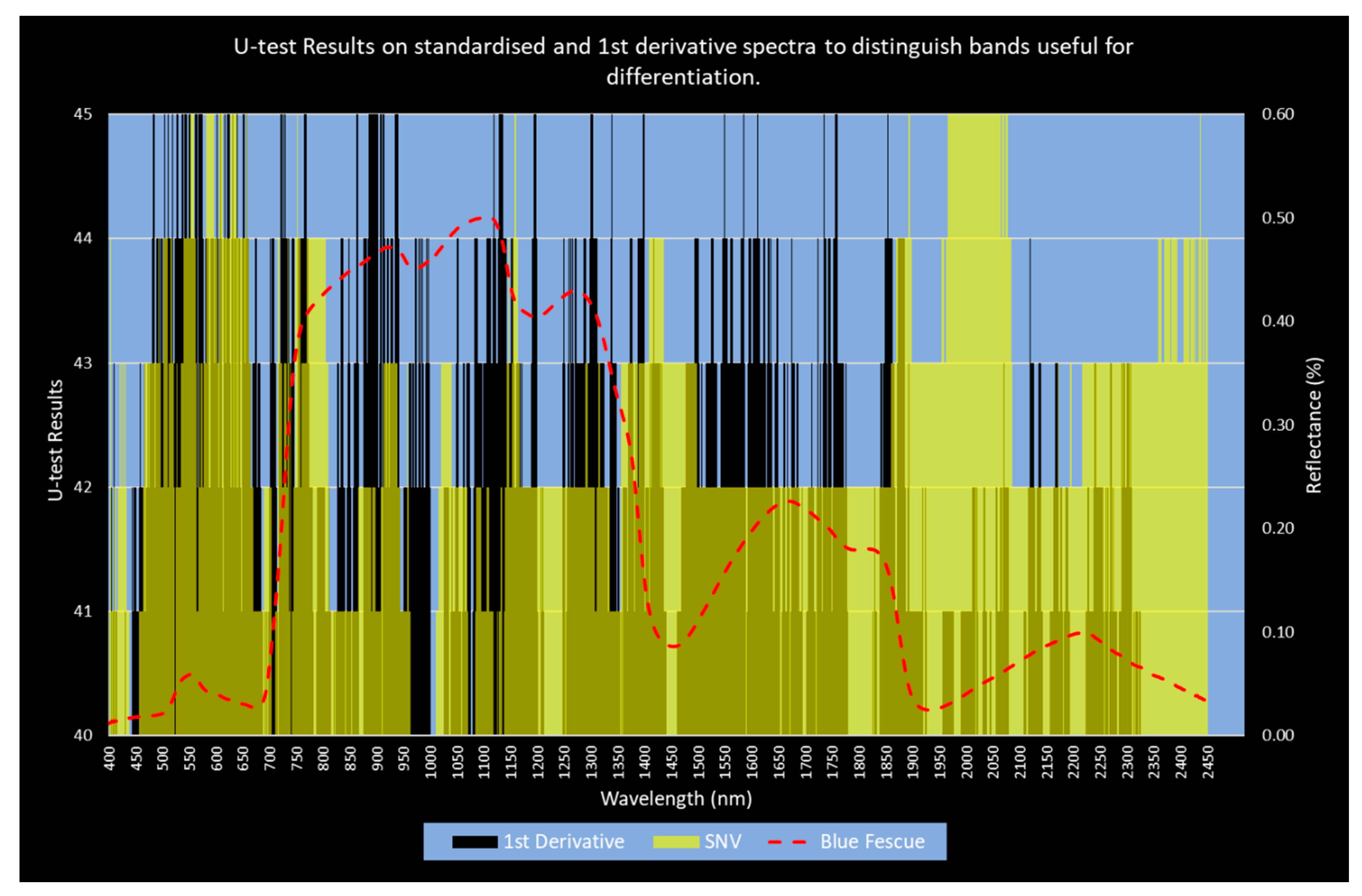
Figure 5 shows the distribution, over the spectrum, of important ranked bands from the U-Test. Important bands are markedly different between the standardized (yellow) and 1st derivative data (black).
The U test from the derivative data indicated a higher importance of VNIR bands, whereas the standardized data highlighted a greater importance of bands in the SWIR.
The U-Test defined 110 1st derivative transformed bands as important, and 148 of the bands were from SNV data. When transformed to the 1st derivative, most of the important bands were identified in the VNIR range of the spectrum. The dramatic change in the distribution of important bands between the two pre-treatments was interesting. The results from the SNV transformation had a greater spread but indicated bands mostly in the SWIR region as important. Table 6 below shows the numbers, distributions, and proportions of each group selected as important.

3.4. Prediction of Sample Collection Time

The reduced training set of 60 samples (30% of the total) resulted in a larger test set (140 samples) for subsequent validation. A successful prediction of collection ‘time’ with an accuracy of >92% was achieved. Table 7 shows the overall accuracy for predicting the collection time associated with each individual subject. Chewings fescue had the lowest overall accuracy at 92.14%.
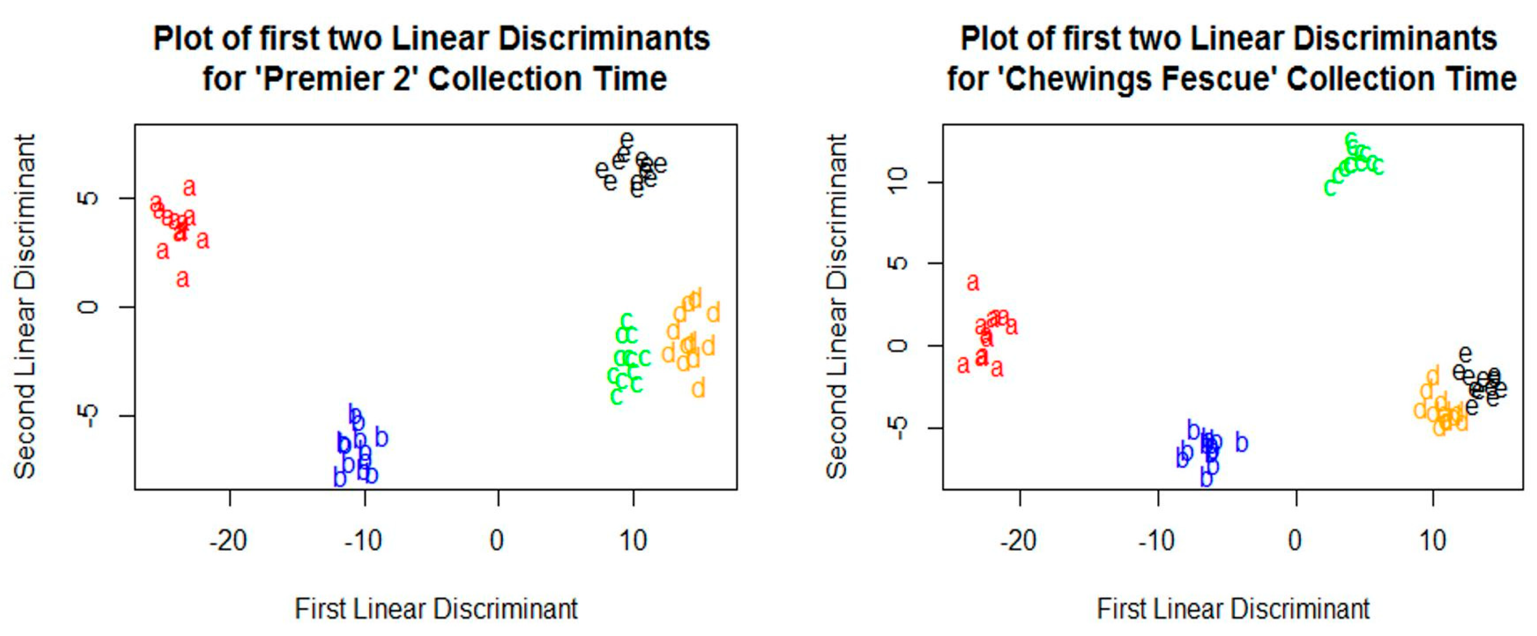
Figure 6 shows a scatter plot for the highest and lowest scoring subjects (‘Premier 2’ and Chewings fescue, respectively). Both show good separability for the early collection times and less separability for the later collection times as plotted in discriminant space. The prediction for sampling at 0800 h was correct with 100% accuracy for all subjects. Later predictions for time of collection showed some variability from one subject to another, with the last two collections (1400 h and 1600 h) misclassified most often.

3.5. Analysis of Collection Time Predictions for Colated Samples

The prediction accuracy for sample time fell to 68.36% (Kappa 60.45%) when the data for all subjects (2000 samples) were combined into a single analysis for collection time. As shown in Table 8, 0800 h (a) and 1200 h (c) were most separable. 1000 h (b) had a spread of predictions before and after the correct time, as did 1400 h (d). The separability problems are illustrated by Figure 7, which shows how categories overlap.

4. Discussions

4.1. Subject Differentiation

The optimum number of bands necessary for subject differentiation varied with the pre-processing method, although both datasets ended up with similar maximum prediction accuracies. The U-test may have contributed to this; Prospere, McLaren [52] reported slightly lower classification accuracies from bands chosen by the U-test, which was consistent across the three methods they used for classification, including LDA. Despite this drawback, in this work, accuracies greater than 95% were achieved with as few as 50 bands. Other studies of species managed to use smaller numbers of bands. For example, Schmidt and Skidmore [26] used six; Prospere, McLaren [52] used around twenty; and Vaiphasa, Skidmore [53] managed with just four. However, the high accuracy in this study extended to the cultivar level. This work supports other studies of reflectance data that have promoted the value of first derivatives to improve analytical results [38,54], but it does contrast with Zhang, Rivard [55], who suggested they may not be suitable for species identification, although the later study was on tree canopies rather than pasture species.

4.2. Band Selection

The bands chosen from the U-Tests produced highly accurate subject predictions. However, these wavelengths may not be the only ones capable of this result [56]. The analyses of species revealed that different bands selected from the two pre-processing methods yielded comparable results. This suggests that the relevant information is widespread in the reflectance bands, supporting the findings of Asner [57], who suggest that bands carrying the pertinent information will vary depending on the species. It is therefore unlikely that a single analysis or group of bands will be usable for all species. For this reason and because the maximum accuracy was achieved with >50 bands, it may be prudent to have a greater number of bands included in a species analysis than previous researchers aspired to use [26,52,53]. The number of bands used and samples collected may require some consideration of the specific variability within the species being examined. Brown, Shepherd [58] suggested it would take more than 5.2 × 10⁹ carefully selected calibration samples to create a comprehensive spectral library for each subject. Care must be taken to avoid the phenomenon known in remote sensing as the Hughes effect, where including too many bands can have a deleterious effect on the prediction accuracy [59]. This drop in accuracy is usually noted when the number of bands is substantially larger than the number of samples and is evident in Table 4 and Table 5, where the accuracy drops with larger amounts of bands included in the analysis.
The techniques and data combined to produce high accuracies for subject determination, even though some of the subjects were closely related cultivars of the same species. This gives promise that the technology could be adapted for persistence trials, if only as a tool to identify those plots that should be attended by experienced agronomists for further scrutiny.

4.3. Band Reduction and Selection

The U test from the derivative data indicated a shift in importance between SWIR and VNIR depending on data pre-treatment. Not having access to data from both regions negates the ability to check this possibility for a specific dataset or task. Cho, Debba [60] did not include any bands from the SWIR region for their study on savannah tree species but suggested some bands in the SWIR might have improved their results. Sobhan, Vaiphasa [61] found important bands for discrimination in the visible part of the spectrum but noted a reduced number of bands in the NIR. They idenitified bands for species descrimination in several regions, including the SWIR, and suggested that bands within these regions ‘share’ information to descriminate species. Our results indicated that both data transformations suggested there were useful bands in the visible range. The derivative transformation suggested very different, important features. This is not unexpected, as derivatives have previously been used to resolve precise features in hyperspectral data [40,62]. Demetriades-Shah, Steven [62] showed the ability of derivatives to suppress background noise, which could explain the narrower features it created and the realization of other features not apparent in the SNV data.

4.4. Diurnal Identification

The lower accuracy achieved when all samples were analyzed suggests that the analysis for individual subjects used slightly different criteria to separate collection times. Plant species and communities are physiologically adapted to specific environments, which enables each to compete in unique circumstances [11]. These environmental forces can pose difficulties with respect to species identification when different species adapt to the same environmental niche (evolutionary convergence) [12].
The challenge our analysis encountered in identifying the collection time for some subjects is interesting because it often occurred in data collected towards the end of the day. This trend only became evident when we reduced the number of samples the model was constructed from. Not all the species exhibited this trait, which points to a possible divergence in physiology. We noted that most of the subjects that were more difficult to categorize later in the day were C3 species, such as the Chewings Fescue example shown in Figure 6, that are less adapted to high-growth competition situations. The other plot in Figure 6 shows the Ryegrass cultivar “Premier 2”, which is more separable and competitive in high-growth environments. This trend is also evident in Figure 7, where all subjects were included in the analysis. It shows the latter two times of day, “d” (2.00 pm) and “e” (4.00 pm), with more overlap than any of the others. This supports the premise that the criteria responsible for change in the spectra throughout the day may have reached an asymptote in some species. This is feasible given the high light conditions experienced during the trial. It is hypothesized that this could relate to a buildup of xanthophyll cycle pigments, photochemical quenching, carbohydrate storage, or a combination of such biophysical properties. The diurnal samples were collected in early spring, which may help explain the inclusion of Kikuyu in the group that was less separable, as the C4 Kikuyu is less active at that time of year [63]. The results are based on limited data but raise intriguing questions around species competition strategies that hyperspectral data may help answer. Further tests with data collected on cloudy days with reduced light levels in comparison to days where sunlight hours are longer (summer) might be a good follow-up study.
The bands chosen by the stepwise feature selection process for this analysis heavily favored bands in the SWIR region. These bands, known to be sensitive to protein, starch, and nutrients in plants [64,65], are thought to enable detection of subtle differences in plant chemistry that change systematically throughout the day, such as carbohydrates.
Although this study was investigating subject separation, in the absence of supplementary data, the lack of additional correlation to plant chemistry became a problem. Plant chemistry, i.e., leaf carbohydrate, nitrogen, fiber, or other variable component concentrations, could have added to the discussion both in terms of species separability and diurnal fluctuation. However, investigating the diurnal fluctuations of plants as measured by reflectance appears to be unique, so comparison with the results from other studies is not possible. The nearest comparison was found to be Gamon, Peñuelas [66], who created the Physiological Reflectance Index (PRI) to measure subtle diurnal fluctuations in photosynthetic efficiency. The goal of this analysis was quite different, as it only sought to identify if it was possible to predict the ‘time’ of a sample collection and was not limited to a 2-band index. It was successful in this respect as collection time was accurately predicted, supporting the use of this equipment for such tasks. The study of Susič, Žibrat [67] found that separating their data into groups according to time of collection improved the overall result accuracy when trying to separate abiotic and biotic drought stress. It therefore seems prudent that diurnal fluctuations should be considered in the experimental setup and data analysis, if not as a category of interest, at least to remove the deleterious effects they introduce to the examination.
The species were well separated, even though diurnal variation was clear. The question of whether individual species can be identified from samples taken under different growth and stress conditions has yet to be fully answered. Price [68] gave a concise list of reasons why it may be difficult or impossible to distinguish any given species from spectra alone, and it has been suggested by others [69,70] that identification may need to be defined by spectra taken at a particular time or growth period to be most effective.
The homogenous nature of the soils within each plot and consistent maintenance between plots, including mowing and watering, reduced the potential variability that might normally be associated with field trials. Those factors, coupled with the use of the CAPP to remove solar variability, contributed to the overall reduction in the variability of the spectral data collected and, thus, likely improved results.
For now, there is still no substitute for expert agronomists in species surveys, and this will likely remain the case for the foreseeable future. Human experts are still the most accurate, but they take a long time to train, which makes them expensive. Add to that the need to include multiple experts to reduce observer error [2], and the cost increases. If hyperspectral analysis technology can be implemented for species identification, it will certainly reduce the burden on those experts since it would be possible to use with minimal training. Therefore, the cost per hour should be a lot lower, making it a cost-effective way to reduce reliance on experts for all tasks. That could allow their effort to be better utilized when it is necessary, for checking equipment accuracy, or to add further value to the hyperspectral results. The added value that hyperspectral differentiation would have is the ability to scale the technology far beyond the capabilities of a human. Analysis of data is only limited by computer speeds, so implementing the analysis of thousands of plots or numerous hectares of land would only be limited by the available data collection technology.
This study faced three primary constraints. Firstly, the absence of wet chemical analysis on the plant samples hindered our ability to link certain observations to plant chemistry, which likely influences variation across species and time of day. Secondly, the small scale of the experimental plots restricted the scope of data collection, preventing a comprehensive, large-scale study. Lastly, the limited geographical diversity due to the experiments being conducted at a single site means we cannot determine the extent to which the findings might vary or remain consistent in different locations. Despite these limitations, the results are promising and hint at the feasibility of this technology to differentiate pasture plants in breeding systems.

5. Conclusions

This research confirms that highly detailed hyperspectral data can be used to differentiate pasture/fine turf species and cultivars and answers the question of whether species similarity and diurnal variation would confound our ability to differentiate them. This supports the hypothesis that it would be possible to differentiate species groups and even cultivars of species only using hyperspectral data. This suggests it would be possible for hyperspectral data to overcome the need for indirect measurements of the persistence trait [1] and allow direct measurement of persistence.
The diurnal variation was discernible, but importantly, it did not preclude species differentiation. Diurnal variation should be a consideration for experimental setups to reduce or negate it as a source of error.
This research provides insight into regions of the spectrum that might assist with species identification or that may be helpful in differentiating subjects. There is still much work needed to enable a practical application, but it is clear from the results that such possibilities exist. The derivative transformed data provided a wider range of useful bands for separation, and importantly, most of them were in the VNIR. This has positive implications for sensor acquisition for such tasks, with the potential to use less expensive variants. Additional research is required to delve deeper into understanding the species-specific mechanisms responsible for the alterations in reflectance. For instance, a comprehensive exploration of the spectral responses of various plant components (e.g., carbohydrates) and physiological processes, such as non-photochemical quenching, could provide valuable insights. By unraveling these intricacies, we can enhance our comprehension of how these factors contribute to changes in reflectance across different plant species and across time. We also suggest that specific field applications of this technology may require adaptation of the method to the specific conditions and requirements. At that stage, an examination of multiple methods would be appropriate to ascertain if LDA is still best suited to the application.

Author Contributions

Conceptualization, T.A.C. and M.C.E.G.; methodology, T.A.C. and M.C.E.G.; software, T.A.C. and M.C.E.G.; validation, T.A.C.; formal analysis, T.A.C. and M.C.E.G.; investigation, T.A.C. and M.C.E.G.; resources, T.A.C. and M.C.E.G.; data curation, T.A.C. and M.C.E.G.; writing—original draft preparation, T.A.C.; writing—review and editing, D.P., T.R. and M.C.E.G.; visualization, T.A.C.; supervision, D.P., T.R. and M.C.E.G.; project administration, M.C.E.G.; funding acquisition, M.C.E.G. All authors have read and agreed to the published version of the manuscript.

Funding

This research was funded as part of the PGP Project: Pioneering to Precision by Ravendsown Limited and the New Zealand Ministry for Primary Industries. Available online: https://www.mpi.govt.nz/funding-and-programmes/primary-growth-partnership/primary-growthpartnership-programmes/pioneering-to-precision-application-of-fertiliser-in-hill-country/, accessed on 22 August 2024.

Data Availability Statement

The data presented in this study are available on request from the corresponding author.

Acknowledgments

The authors would like to acknowledge and thank the NZSTI for their support by allowing data collection from their trial plots. The authors would also like to acknowledge the support of Massey University and AgResearch Ltd. for their support of this work.

Conflicts of Interest

Author T. A. Cushnahan is currently employed by the Crown Research Institute, AgResearch Ltd., but all fieldwork and data analysis was carried out while researching a PhD at Massey University. The remaining authors declare that the research was conducted in the absence of any commercial or financial relationships that could be construed as a potential conflict of interest.

References

  1. Dodd, M.B.; Chapman, D.F.; Ludemann, C.I.; Griffiths, W.; Tozer, K.N.; Donnelly, L. The measurement of perennial ryegrass persistence. J. N. Z. Grassl. 2018, 80, 161–168. [Google Scholar] [CrossRef]
  2. Morrison, L.W. Observer error in vegetation surveys: A review. J. Plant Ecol. 2015, 9, 367–379. [Google Scholar] [CrossRef]
  3. Schaaf, C.B.; Strahler, A.H. Solar zenith angle effects on forest canopy hemispherical reflectances calculated with a geometric-optical bidirectional reflectance model. IEEE Trans. Geosci. Remote Sens. 1993, 31, 921–927. [Google Scholar] [CrossRef]
  4. Middleton, E.M. Solar zenith angle effects on vegetation indices in tallgrass prairie. Remote Sens. Environ. 1991, 38, 45–62. [Google Scholar] [CrossRef]
  5. Huete, A.R. Soil and sun angle interactions on partial canopy spectra. Int. J. Remote Sens. 1987, 8, 1307–1317. [Google Scholar] [CrossRef]
  6. Ma, X.; Huete, A.; Tran, N.N.; Bi, J.; Gao, S.; Zeng, Y. Sun-Angle Effects on Remote-Sensing Phenology Observed and Modelled Using Himawari-8. Remote Sens. 2020, 12, 1339. [Google Scholar] [CrossRef]
  7. Jafarbiglu, H.; Pourreza, A. Impact of sun-view geometry on canopy spectral reflectance variability. ISPRS J. Photogramm. Remote Sens. 2023, 196, 270–286. [Google Scholar] [CrossRef]
  8. Pinter, P.J.; Jackson, R.D.; Idso, S.B.; Reginato, R.J. Diurnal patterns of wheat spectral reflectances. IEEE Trans. Geosci. Remote Sens. 1983, 2, 156–163. [Google Scholar] [CrossRef]
  9. Graf, A.; Schlereth, A.; Stitt, M.; Smith, A.M. Circadian control of carbohydrate availability for growth in Arabidopsis plants at night. Proc. Natl. Acad. Sci. USA 2010, 107, 9458–9463. [Google Scholar] [CrossRef]
  10. Horton, P.; Ruban, A.V.; Walters, R.G. Regulation of light harvesting in green plants. Annu. Rev. Plant Physiol. Plant Mol. Biol. 1996, 47, 655–684. [Google Scholar] [CrossRef]
  11. Grime, J.P.; Thompson, K.; Hunt, R.; Hodgson, J.G.; Cornelissen, J.H.C.; Rorison, I.H.; Hendry, G.A.F.; Ashenden, T.W.; Askew, A.P.; Band, S.R.; et al. Integrated screening validates primary axes of specialisation in plants. Oikos 1997, 79, 259–281. [Google Scholar] [CrossRef]
  12. Ollinger, S. Sources of variability in canopy reflectance and the convergent properties of plants. New Phytol. 2011, 189, 375–394. [Google Scholar] [CrossRef] [PubMed]
  13. Girolamo-Neto, C.D.; Sanches, I.D.A.; Neves, A.K.; Prudente, V.H.R.; Körting, T.S.; Picoli, M.C.A.; Aragão, L.E.O.e.C.d. Assessment of texture features for bermudagrass (cynodon dactylon) detection in sugarcane plantations. Drones 2019, 3, 36. [Google Scholar] [CrossRef]
  14. Wang, C.; Hunt, E.R.; Zhang, L.; Guo, H. Phenology-assisted classification of C3 and C4 grasses in the U.S. Great Plains and their climate dependency with MODIS time series. Remote Sens. Environ. 2013, 138, 90–101. [Google Scholar] [CrossRef]
  15. Lilienthal, H.; Wilde, P.; Schnug, E. Proximal hyperspectral sensing in plant breeding. In Proceedings of the 13th International Conference on Precision Agriculture, St. Louis, MI, USA, 31 July–3 August 2016. [Google Scholar]
  16. Araus, J.L.; Cairns, J.E. Field high-throughput phenotyping: The new crop breeding frontier. Trends Plant Sci. 2014, 19, 52–61. [Google Scholar] [CrossRef]
  17. Walter, A.; Studer, B.; Kölliker, R. Advanced phenotyping offers opportunities for improved breeding of forage and turf species. Ann. Bot. 2012, 110, 1271–1279. [Google Scholar] [CrossRef]
  18. Ghamkhar, K. Phenomics for the Improvement of Crop Adaptation. In Plant Genetic Resources for the 21st Century, 1st ed.; Apple Academic Press: Palm Bay, FL, USA, 2023; pp. 115–129. ISBN 9781003302957. [Google Scholar]
  19. Caturegli, L.; Lulli, F.; Foschi, L.; Guglielminetti, L.; Bonari, E.; Volterrani, M. Turfgrass spectral reflectance: Simulating satellite monitoring of spectral signatures of main C3 and C4 species. Precis. Agric 2015, 16, 297–310. [Google Scholar] [CrossRef]
  20. Irisarri, J.; Oesterheld, M.; Verón, S.; Paruelo, J. Grass species differentiation through canopy hyperspectral reflectance. Int. J. Remote Sens. 2009, 30, 5959–5975. [Google Scholar] [CrossRef]
  21. Caturegli, L.; Corniglia, M.; Gaetani, M.; Grossi, N.; Magni, S.; Migliazzi, M.; Angelini, L.; Mazzoncini, M.; Silvestri, N.; Fontanelli, M. Unmanned aerial vehicle to estimate nitrogen status of turfgrasses. PLoS ONE 2016, 11, e0158268. [Google Scholar] [CrossRef]
  22. Caturegli, L.; Gaetani, M.; Volterrani, M.; Magni, S.; Minelli, A.; Baldi, A.; Brandani, G.; Mancini, M.; Lenzi, A.; Orlandini, S. Normalized Difference Vegetation Index versus Dark Green Colour Index to estimate nitrogen status on bermudagrass hybrid and tall fescue. Int. J. Remote Sens. 2020, 41, 455–470. [Google Scholar] [CrossRef]
  23. Caturegli, L.; Matteoli, S.; Gaetani, M.; Grossi, N.; Magni, S.; Minelli, A.; Corsini, G.; Remorini, D.; Volterrani, M. Effects of water stress on spectral reflectance of bermudagrass. Sci. Rep. 2020, 10, 15055. [Google Scholar] [CrossRef]
  24. Marín, J.; Yousfi, S.; Mauri, P.V.; Parra, L.; Lloret, J.; Masaguer, A. RGB vegetation indices, NDVI, and biomass as indicators to evaluate C3 and C4 turfgrass under different water conditions. Sustainability 2020, 12, 2160. [Google Scholar] [CrossRef]
  25. Fotia, K.; Ntoulas, N.; Koliopanos, C.; Tsirogiannis, I.; Nektarios, P. Utilization of reflectance indices to evaluate the impact of grey or recycled irrigation water on Festuca arundinacea turfgrass. In Proceedings of the International Symposium on Sensing Plant Water Status-Methods and Applications in Horticultural Science 1197, Potsdam, Germany, 5−7 October 2016; pp. 103–108. [Google Scholar]
  26. Schmidt, K.S.; Skidmore, A.K. Spectral discrimination of vegetation types in a coastal wetland. Remote Sens. Environ. 2003, 85, 92–108. [Google Scholar] [CrossRef]
  27. Möckel, T.; Dalmayne, J.; Schmid, B.; Prentice, H.; Hall, K. Airborne Hyperspectral Data Predict Fine-Scale Plant Species Diversity in Grazed Dry Grasslands. Remote Sens. 2016, 8, 133. [Google Scholar] [CrossRef]
  28. Carter, G.A.; Knapp, A.K.; Anderson, J.E.; Hoch, G.A.; Smith, M.D. Indicators of plant species richness in AVIRIS spectra of a mesic grassland. Remote Sens. Environ. 2005, 98, 304–316. [Google Scholar] [CrossRef]
  29. Davidson, A.; Csillag, F. A comparison of three approaches for predicting C4 species cover of northern mixed grass prairie. Remote Sens. Environ. 2003, 86, 70–82. [Google Scholar] [CrossRef]
  30. Liu, L.; Cheng, Z. Mapping C3 and C4 plant functional types using separated solar-induced chlorophyll fluorescence from hyperspectral data. Int. J. Remote Sens. 2011, 32, 9171–9183. [Google Scholar] [CrossRef]
  31. Sims, D.A.; Gamon, J.A. Relationships between leaf pigment content and spectral reflectance across a wide range of species, leaf structures and de-velopmental stages. Remote Sens. Environ. 2002, 81, 337–354. [Google Scholar] [CrossRef]
  32. Hull, R.J. Energy relations and carbohydrate partitioning in turfgrasses. Turfgrass 1992, 32, 175–205. [Google Scholar]
  33. Sanches, I.D.A. Hyperspectral Proximal Sensing of the Botanical Composition and Nutrient Content of New Zealand Pastures: A Thesis Presented in Partial Fulfilment of the Requirements for the Degree of Doctor of Philosophy in Earth Science. Ph.D. Thesis, Massey University, Palmerston North, New Zealand, 2009. [Google Scholar]
  34. Sanches, I.; Tuohy, M.; Hedley, M.; Bretherton, M. Large, durable and low-cost reflectance standard for field remote sensing applications. Int. J. Remote Sens. 2009, 30, 2309–2319. [Google Scholar] [CrossRef]
  35. Pu, R. Broadleaf species recognition with in situ hyperspectral data. Int. J. Remote Sens. 2009, 30, 2759–2779. [Google Scholar] [CrossRef]
  36. Lu, Y.; Saeys, W.; Kim, M.; Peng, Y.; Lu, R. Hyperspectral imaging technology for quality and safety evaluation of horticultural products: A review and celebration of the past 20-year progress. Postharvest Biol. Technol. 2020, 170, 111318. [Google Scholar] [CrossRef]
  37. Barnes, R.; Dhanoa, M.; Lister, S.J. Standard normal variate transformation and de-trending of near-infrared diffuse reflectance spectra. Appl. Spectrosc. 1989, 43, 772–777. [Google Scholar] [CrossRef]
  38. Penuelas, J.; Gamon, J.A.; Fredeen, A.L.; Merino, J.; Field, C.B. Reflectance Indexes Associated with Physiological-Changes in Nitrogen-Limited and Water-Limited Sunflower Leaves. Remote Sens. Environ. 1994, 48, 135–146. [Google Scholar] [CrossRef]
  39. Rubo, S.; Zinkernagel, J. Exploring hyperspectral reflectance indices for the estimation of water and nitrogen status of spinach. Biosyst. Eng. 2022, 214, 58–71. [Google Scholar] [CrossRef]
  40. Tsai, F.; Philpot, W. Derivative Analysis of Hyperspectral Data. Remote Sens. Environ. 1998, 66, 41–51. [Google Scholar] [CrossRef]
  41. Stevens, A.; Ramirez–Lopez, L. An Introduction to the Prospectr Package. R Package Vignette. 2014, Version 0.1.3. Available online: https://cran.r-project.org/web/packages/prospectr/index.html (accessed on 19 August 2024).
  42. Welling, M. Fisher Linear Discriminant Analysis; Department of Computer Science, University of Toronto: Toronto, STC, Canada, 2006; p. 3. [Google Scholar]
  43. Hastie, T.; Tibshirani, R.; Friedman, J.H. The Elements of Statistical Learning: Data Mining, Inference, and Prediction, 2nd ed.; Springer series in statistics; Springer: New York, NY, USA, 2009. [Google Scholar]
  44. Bhardwaj, A.; Verma, P. A Textbook on Pattern Recognition; Alpha Science International: Oxford, UK, 2015. [Google Scholar]
  45. Lu, J.; Plataniotis, K.N.; Venetsanopoulos, A.N. Face recognition using LDA-based algorithms. IEEE Trans. Neural Netw. 2003, 14, 195–200. [Google Scholar] [PubMed]
  46. Dudoit, S.; Fridlyand, J.; Speed, T.P. Comparison of discrimination methods for the classification of tumors using gene expression data. J. Am. Stat. Assoc. 2002, 97, 77–87. [Google Scholar] [CrossRef]
  47. Acquah, G.E.; Via, B.K.; Billor, N.; Fasina, O.O.; Eckhardt, L.G. Identifying plant part composition of forest logging residue using infrared spectral data and linear discriminant analysis. Sensors 2016, 16, 1375. [Google Scholar] [CrossRef]
  48. Wu, W.; Mallet, Y.; Walczak, B.; Penninckx, W.; Massart, D.; Heuerding, S.; Erni, F. Comparison of regularized discriminant analysis linear discriminant analysis and quadratic discriminant analysis applied to NIR data. Anal. Chim. Acta 1996, 329, 257–265. [Google Scholar] [CrossRef]
  49. Bioucas-Dias, J.M.; Plaza, A.; Camps-Valls, G.; Scheunders, P.; Nasrabadi, N.; Chanussot, J. Hyperspectral remote sensing data analysis and future challenges. IEEE Geosci. Remote Sens. Mag. 2013, 1, 6–36. [Google Scholar] [CrossRef]
  50. Bandos, T.V.; Bruzzone, L.; Camps-Valls, G. Classification of hyperspectral images with regularized linear discriminant analysis. IEEE Trans. Geosci. Remote Sens. 2009, 47, 862–873. [Google Scholar] [CrossRef]
  51. Weihs, C.; Ligges, U.; Luebke, K.; Raabe, N. klaR Analyzing German Business Cycles. In Data Analysis and Decision Support; Baier, D., Decker, R., Schmidt-Thieme, L., Eds.; Springer: Berlin/Heidelberg, Germany, 2005; pp. 335–343. [Google Scholar]
  52. Prospere, K.; McLaren, K.; Wilson, B. Plant Species Discrimination in a Tropical Wetland Using In Situ Hyperspectral Data. Remote Sens. 2014, 6, 8494–8523. [Google Scholar] [CrossRef]
  53. Vaiphasa, C.; Skidmore, A.K.; de Boer, W.F.; Vaiphasa, T. A hyperspectral band selector for plant species discrimination. ISPRS J. Photogramm. Remote Sens. 2007, 62, 225–235. [Google Scholar] [CrossRef]
  54. Cho, M.A.; Skidmore, A.K. A new technique for extracting the red edge position from hyperspectral data: The linear extrapolation method. Remote Sens. Environ. 2006, 101, 181–193. [Google Scholar] [CrossRef]
  55. Zhang, J.; Rivard, B.; Sánchez-Azofeifa, A.; Castro-Esau, K. Intra- and inter-class spectral variability of tropical tree species at La Selva, Costa Rica: Implications for species identification using HYDICE imagery. Remote Sens. Environ. 2006, 105, 129–141. [Google Scholar] [CrossRef]
  56. Huberty, C.J. Issues in the use and interpretation of discriminant analysis. Psychol. Bull. 1984, 95, 156–171. [Google Scholar] [CrossRef]
  57. Asner, G.P. Biophysical and Biochemical Sources of Variability in Canopy Reflectance. Remote Sens. Environ. 1998, 64, 234–253. [Google Scholar] [CrossRef]
  58. Brown, D.J.; Shepherd, K.D.; Walsh, M.G.; Mays, M.D.; Reinsch, T.G. Global soil characterization with VNIR diffuse reflectance spectroscopy. Geoderma 2006, 132, 273–290. [Google Scholar] [CrossRef]
  59. Hughes, G. On the mean accuracy of statistical pattern recognizers. Inf. Theory IEEE Trans. 1968, 14, 55–63. [Google Scholar] [CrossRef]
  60. Cho, M.A.; Debba, P.; Mathieu, R.; Naidoo, L.; van Aardt, J.; Asner, G.P. Improving discrimination of savanna tree species through a multiple-endmember spectral angle mapper approach: Canopy-level analysis. Geosci. Remote Sens. IEEE Trans. 2010, 48, 4133–4142. [Google Scholar] [CrossRef]
  61. Sobhan, I.; Vaiphasa, C.; Skidmore, A. Spectral regions for maximizing species discrimination. Species Discrimination Hyperspectral Perspective. 2007, pp. 35–37. Available online: https://www.google.com/search?q=Species+discrimination+from+a+hyperspectral+perspective&oq=Species+discrimination+from+a+hyperspectral+perspective&gs_lcrp=EgZjaHJvbWUyBggAEEUYOTIGCAEQRRg8MgYIAhBFGDzSAQczMjNqMGo0qAIAsAIB&sourceid=chrome&ie=UTF-8 (accessed on 19 August 2024).
  62. Demetriades-Shah, T.H.; Steven, M.D.; Clark, J.A. High resolution derivative spectra in remote sensing. Remote Sens. Environ. 1990, 33, 55–64. [Google Scholar] [CrossRef]
  63. Betteridge, K.; Haynes, D. Altering the growth pattern of kikuyu pastures with temperate grasses. In Proceedings of the Proceedings of the New Zealand Grassland Association, Whangarei, New Zealand, 1 January 1986; pp. 149–156. [Google Scholar]
  64. Axelsson, C.; Skidmore, A.K.; Schlerf, M.; Fauzi, A.; Verhoef, W. Hyperspectral analysis of mangrove foliar chemistry using PLSR and support vector regression. Int. J. Remote Sens. 2013, 34, 1724–1743. [Google Scholar] [CrossRef]
  65. Curran, P.J. Remote sensing of foliar chemistry. Remote Sens. Environ. 1989, 30, 271–278. [Google Scholar] [CrossRef]
  66. Gamon, J.A.; Peñuelas, J.; Field, C.B. A narrow-waveband spectral index that tracks diurnal changes in photosynthetic efficiency. Remote Sens. Environ. 1992, 41, 35–44. [Google Scholar] [CrossRef]
  67. Susič, N.; Žibrat, U.; Širca, S.; Strajnar, P.; Razinger, J.; Knapič, M.; Vončina, A.; Urek, G.; Gerič Stare, B. Discrimination between abiotic and biotic drought stress in tomatoes using hyperspectral imaging. Sens. Actuators B Chem. 2018, 273, 842–852. [Google Scholar] [CrossRef]
  68. Price, J.C. How unique are spectral signatures? Remote Sens. Environ. 1994, 49, 181–186. [Google Scholar] [CrossRef]
  69. Sobhan, M.I. Species Discrimination from a Hyperspectral Perspective; Wageningen University and Research: Wageningen, The Netherlands, 2007. [Google Scholar]
  70. Cole, B.; McMorrow, J.; Evans, M. Spectral monitoring of moorland plant phenology to identify a temporal window for hyperspectral remote sensing of peatland. ISPRS J. Photogramm. Remote Sens. 2014, 90, 49–58. [Google Scholar] [CrossRef]
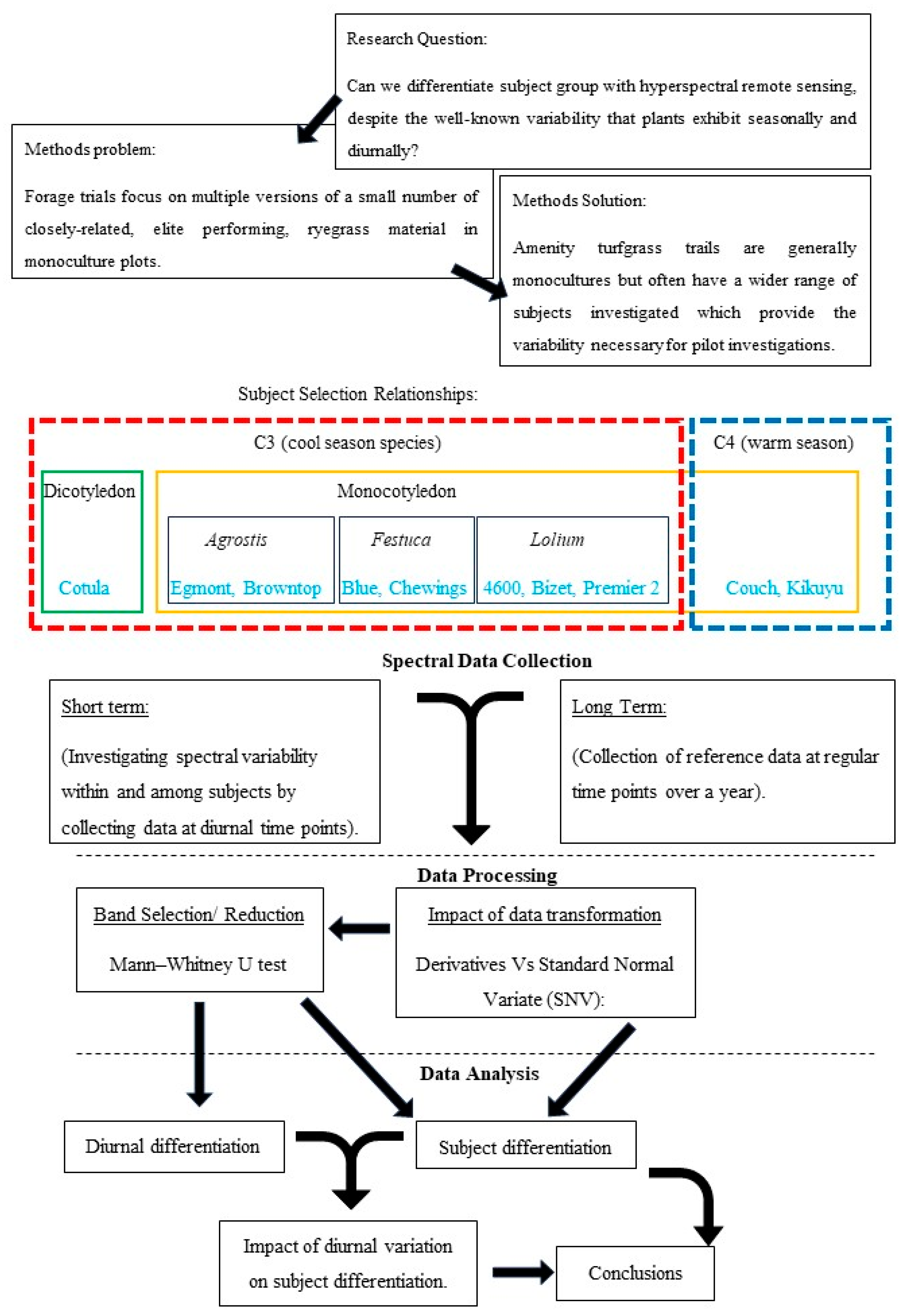
Figure 1. Research flow chart outlining the rationale and research story.
Remotesensing 16 03142 g001
Figure 2. Ryegrass ‘Bizet’ plot showing locational pegs and a graphic (black line, 32 cm diameter) showing how the CAPP was located within the pegs.
Remotesensing 16 03142 g002
Figure 3. Average unmodified reflectance for the 280 samples for each of the 10 subjects.
Remotesensing 16 03142 g003
Figure 4. Average of the 1st derivative of reflectance for each of the 10 subjects.
Remotesensing 16 03142 g004
Figure 5. Frequency plot of U-test results for standardized spectra and 1st derivative transformed spectra with a significance level of 5% from standardized data. The reflectance curve of Blue Fescue is overlaid for visualization of typical reflectance features. The y axis represents the cumulative total of positive results when each subject is compared against every other subject at a given wavelength.
Remotesensing 16 03142 g005
Figure 6. Plot of the first two linear discriminants for ‘Premier 2’ and ‘Chewings fescue’ (n = 200). a = 0800 h, b = 1000 h, c = 1200 h, d = 1400 h and e = 1600 h. The times are also color coded for added clarity.
Remotesensing 16 03142 g006
Figure 7. Plot of the first two linear discriminants for the time of collection when all subject data were collated and analyzed together. a = 0800 h, b = 1000 h, c = 1200 h, d = 1400 h and e = 1600 h. The times are also color coded for added clarity.
Remotesensing 16 03142 g007
Table 1. Common and botanical names of subjects chosen for inclusion in the trial.
Common NameLatin Name
CotulaLeptinella dioica cv. Pahia
CouchCynodon dactylon cv. Agridark
KikuyuPennisetum clandestinum cv. Regal Stay Green
EgmontAgrostis capillaris var. Egmont
BrowntopAgrostis capillaris cv. Arrowtown
Ryegrass ‘4600’Lolium perenne cv. 4600
Ryegrass ‘Bizet’Lolium perenne cv. Bizet
Ryegrass ‘Premier 2’Lolium perenne cv. Premier 2
Blue FescueFestuca sp.
Chewing’s FescueFestuca rubra subsp. Commutata
Table 2. Example confusion matrix and basic statistics for LDA used to differentiate subjects. Analysis carried out on 12 bands of SNV transformed spectra and defined as important by the U-Test. Overall accuracy is defined as the total correct (sum of diagonals) divided by the total samples.
Reference Sample
Blue FescueBrowntopChewings FescueCotulaCouchEgmontKikuyuRyegrass—4600Ryegrass—BizetRyegrass—Premier 2
LDA PredictionBlue Fescue50274023000
Browntop04420020000
Chewings Fescue03340010010
Cotula01246000000
Couch00015200000
Egmont05201500502
Kikuyu00121049000
Ryegrass—460010002102446
Ryegrass—Bizet50820047509
Ryegrass—Premier 2010100020139
Overall Statistics
Accuracy:0.7821
95% Confidence Interval:(0.7456, 0.8157)
No Information Rate:0.1
p-Value [Acc > NIR]:<2.2 × 10⁻¹⁶
Kappa:0.7579
Table 3. Example confusion matrix and basic statistics for LDA used to identify species. Analysis carried out on 11 bands of spectra transformed to the 1st derivative and defined as important by the U-Test.
Reference Sample
Blue FescueBrowntopChewings Fescue CotulaCouchEgmontKikuyuRyegrass—4600Ryegrass—BizetRyegrass—Premier 2
LDA PredictionBlue Fescue34320521221
Browntop05010040000
Chewings Fescue62480220001
Cotula00154000000
Couch50204600262
Egmont00001470000
Kikuyu00000054000
Ryegrass—460001000104313
Ryegrass—Bizet500020164313
Ryegrass—Premier 260220003436
Overall Statistics
Accuracy:0.8125
95% Confidence Interval:(0.7777, 0.844)
No Information Rate:0.1
p-Value [Acc > NIR]:<2.2 × 10⁻¹⁶
Kappa:0.7917
Table 4. Summary of LDA subject prediction accuracy results using standardized data with increasing numbers of bands chosen via the U-Test.
Bands Used127615020040480091417402050
Accuracy78.21%89.82%91.61%93.75%96.96%96.07%94.20%92.14%93.04%
kappa75.79%88.69%90.67%93.06%96.63%95.63%94.25%91.27%92.26%
Table 5. Summary LDA subject prediction accuracy results using 1st derivative data with increasing numbers of bands chosen via the U-Test.
Bands Used115011026642281411771665
Accuracy81.25%95.54%96.61%98.04%97.68%96.96%96.07%94.82%
kappa79.17%95.04%96.23%97.82%97.42%96.63%95.63%94.25%
Table 6. Number of important bands for subject separation, identified by U-Test, for each transformation and broken down by spectral region. The VNIR range was 400 nm to 1000 nm, the SWIR range was from 1000 nm to 2500 nm, and the total range was from 400 nm to 2500 nm.
Group DetailsImportant BandsBands in RangeImportance as a Proportion of the Group
1st derivative (total)1102020 bands5.4%
SNV (total)1482051 bands7.3%
1st derivative (VNIR only)981000 bands9.8%
SNV (VNIR only)411000 bands4.1%
1st derivative (SWIR only)131020 bands1.3%
SNV (SWIR only)1071051 bands10.2%
Table 7. LDA prediction accuracy for the time of data collection (by subject).
Target SubjectPrediction AccuracyKappa
Blue Fescue97.86%97.86%
Browntop95.71%95.71%
Chewings92.14%92.14%
Cotula98.57%98.57%
Couch94.29%94.29%
Egmont96.43%96.43%
Kikuyu98.57%98.57%
Ryegrass—‘4600’97.86%97.86%
Ryegrass—‘Bizet’94.29%94.29%
Ryegrass—‘Premier 2’100.00%100.00%
Table 8. The confusion matrix for collection time prediction when using all data (accuracy 68.36%, Kappa 60.45%) (n = 2000). Time = (a) 08.00 (b) 10.00 (c) 12.00 (d) 14.00 (e) 16.00.
Reference
Predictionabcde
a25771026
b815828182
c02422598
d12025172119
e147279145
Disclaimer/Publisher’s Note: The statements, opinions and data contained in all publications are solely those of the individual author(s) and contributor(s) and not of MDPI and/or the editor(s). MDPI and/or the editor(s) disclaim responsibility for any injury to people or property resulting from any ideas, methods, instructions or products referred to in the content.