A Study of the Effect of DEM Spatial Resolution on Flood Simulation in Distributed Hydrological Modeling

Abstract

Watershed hydrological modeling methods are currently the predominant approach for flood forecasting. Digital elevation model (DEM) data, a critical input variable, significantly influence the accuracy of flood simulations, primarily due to their resolution. However, there is a paucity of research exploring the relationship between DEM resolution and flood simulation accuracy. This study aims to investigate this relationship by examining three watersheds of varying scales in southern Jiangxi Province, China. Utilizing the Liuxihe model, a new-generation physically based distributed hydrological model (PBDHM), we collected and collated data, including DEM, land use, soil type, and hourly flow and rainfall data from monitoring stations, covering 22 flood events over the last decade, to conduct model calibration and flood simulation. DEM data were processed into seven resolutions, ranging from 30 m to 500 m, to analyze the impact of DEM resolution on flood simulation accuracy. The results are as follows. (1) The Nash–Sutcliffe efficiency coefficients for the entire set of flood events were above 0.75, demonstrating the Liuxihe model’s strong applicability in this region. (2) The DEM resolution of the Anhe and Dutou watersheds lost an average of 7.9% and 0.8% accuracy when increasing from 30 m to 200 m, with further losses of 37.9% and 10.7% from 200 m to 300 m. Similarly, the Mazhou watershed showed an average of 8.4% accuracy loss from 30 m to 400 m and 20.4% from 400 m to 500 m. These results suggest a threshold where accuracy sharply declines as DEM resolution increases, and this threshold rises with watershed scale. (3) Parameter optimization in the Liuxihe model significantly enhanced flood simulation accuracy, effectively compensating for the reduction in accuracy caused by increased DEM resolution. (4) The optimal parameters for flood simulation varied with different DEM resolutions, with significant changes observed in riverbed slope and river roughness, which are highly sensitive to DEM resolution. (5) Changes in DEM resolution did not significantly impact surface flow production. However, the extraction of the water system and the reduction in slope were major factors contributing to the decline in flood simulation accuracy. Overall, this study elucidates that there is a threshold range of DEM resolution that balances data acquisition efficiency and computational speed while satisfying the basic requirements for flood simulation accuracy. This finding provides crucial decision-making support for selecting appropriate DEM resolutions in hydrological forecasting.

1. Introduction

Flooding is one of the natural disasters with the heaviest impacts and losses, posing a major threat to the safety of people’s lives and property, while severely restricting local economic development [1,2,3]. Flood forecasting is simulating the future flood process according to the law of flood generation and movement, which is an important content of the current flood control non-engineering measures [4,5,6]. Watershed hydrological modeling is the mainstream method for flood forecasting [7,8], and hydrological models can be divided into lumped, semi-distributed and fully distributed physically hydrological models according to the stage of development [9,10]. The structure of lumped models is relatively simple, with representative models such as the Stanford model [11], the HBV model [12], the Sac model [13], the Xin’an Jiang model [14], etc. Semi-distributed hydrological models consider dividing the whole watershed into cells, but the cell grids are large, with representative models such as TOPMODEL [15], SWAT [16] and HEC-HMS [17]. In recent years, with the breakthroughs in computer technology, RS technology, GIS technology and radar rainfall measurement technology, physically based distributed hydrological models (PBDHMs) have been rapidly developed, which have obvious advantages in the theoretical basis of refined runoff simulation because of their strict physical mechanisms. It is an inevitable trend for the development of watershed hydrological stimulation in the future, and the representative models are the SHE model [18], the VFLO model [19], the VIC model [20], and the Liuxihe model [21], etc.

DEM (digital elevation model) data are an important input for PBDHMs, and contain important subsurface features. With the help of the D8 algorithm, the flow direction, catchment accumulation, and water system of a watershed are extracted in order. DEM data of different spatial resolution will affect the extraction of the water system of a watershed, which will then have an impact on the flood simulation accuracy of the watershed [22,23,24]. Many scholars have also researched the influence of different DEM resolutions on flood simulation results. Li Jianzhu et al. [25] obtained 10 sets of DEMs with 1–30 m resolution based on UAV 3D tilt photography with 7 cm representing high resolution and ASTER 30 m resampling, and constructed an HEC-HMS model for hydrological simulation, which showed that the Nash–Sutcliffe efficiency coefficient was slightly higher for the high resolution, but there was little difference in the overall simulation results of the flooding processes at other resolutions. Dixon et al. [26] found that the SWAT model is sensitive to the source of the DEM data, and considered that the effects of resolution of DEMs in watershed modeling cannot be ignored. Rocha et al. [27] used the SWAT model to assess the accuracy of hydrological response of low-elevation forested watersheds under the influence of 1 m-, 10 m-, and 30 m-resolution DEMs, and the results showed that the higher the resolution of the DEMs, the better the performance of the model. Suliman et al. [28] resampled the ASTER 30 m DEMs to generate a total of 10 resolutions from 30 to 300 m, and constructed TOPMODEL for hydrological simulation in Malaysia. The results showed that the difference in resolution significantly affects the terrain index distribution, while the runoff simulation accuracy decreases with the resolution. Cotter et al. [29] suggested that DEM data with greater resolution would reduce watershed area and slope and increase slope length, and that the minimum resolution of the GIS data entered for a model output error of less than 10% depends on the output variable of interest. Li Jing et al. [30] established several DEM datasets with different data sources and resolutions, and the results showed that a DEM with higher resolution can obtain a more accurate simulation of the flood peak, but the highest-resolution data may not necessarily provide the best flood simulation results. Simon et al. [31] investigated the effect of the vertical accuracy of DEM on runoff simulation using TOPMODEL. The results showed that DEM resolution has an important effect on hydrological simulation performance, which can be compensated by model calibration. Yufang Gao et al. [32] used ASTER 30 m DEM, SRTM 90 m DEM and resampled DEM (40 m, 50 m, 60 m, 70 m, 80 m and 90 m) for hydrological simulation using the HEC-HMS model, and the results showed that the model based on SRTM 90 m had the best coefficient of determinism.

Theoretically, the higher the resolution of the DEM, the finer the details of the geographical elements it expresses, but as noted by other scholars, the highest resolution does not necessarily produce the best simulation results, and for watershed objects at different scales, the differentiation in flood simulation accuracies caused by the change in resolution is a difficult problem that needs to be further investigated.

Lumped hydrological models consider a watershed as a whole, which makes it difficult to address non-uniformity in spatial distribution of the watershed’s physical characteristics, so it is necessary to determine the model parameters by the rate of the measured data [33]. Semi-distributed hydrological models have a large grid, which cannot accurately express the spatial changes in a watershed’s sub-watershed topography, and the catchment computation is mainly based on hydrological algorithms with low computational accuracy [34]. PBDHMs can fully reflect spatial changes in the physical characteristics of a watershed, determine the model parameters from physical mechanisms, and utilize grid-based rainfall data with high spatial and temporal resolution to simulate runoff. Most of the previous studies have used aggregate or semi-distributed hydrological models to test the effect of different-resolution DEMs on flood simulation [25,26,27,28,31,32,35], and all of them focused exclusively on examining the impact of DEM resolution on flood simulation within a single-scale watershed.

The drastic impacts of global climate change and human activities have led to more frequent flooding events. Consequently, understanding the relationship between DEM resolution and simulation accuracy has become an urgent issue in flood forecasting. This study aims to address this challenge. In this study, we implemented innovations such as distributed hydrological modeling, comparative analysis of catchments of varying scales, and investigation of hydrological model parameter variations across different DEM resolutions. The study area comprised three watersheds—Anhe, Dutou, and Mazhou—in southern Jiangxi Province, China. DEM data were resampled at seven spatial resolutions, 30 m, 90 m, 150 m, 200 m, 300 m, 400 m, and 500 m, to construct a Liuxihe model for flood simulation. We used the stand-alone software CYB.LMS 2.0 for flood simulation [36,37], and the objectives were: (1) to test the applicability of the Liuxihe model in the south of Jiangxi Province; (2) to compare the impacts of different DEM spatial resolutions on flood simulation accuracy; (3) to examine whether the parameters of PBDHMs exhibit spatial scale effects in response to different resolutions; and (4) to explore why different spatial resolutions lead to changes in flood simulation accuracy.

2. Materials and Methods

2.1. Study Area

The Anhe, Dutou, and Mazhou watersheds in Ganzhou City, Jiangxi Province, China, were selected to evaluate the applicability of the Liuxihe model and assess the impact of different DEM resolutions on flood simulation. These watersheds, located in the upper reaches of the Gan River (a primary tributary of the Yangtze River), feature mountainous and hilly topography and experience a subtropical monsoon climate with abundant rainfall and a long frost-free period. During summer, influenced by the southwestern airflow at the edge of the subtropical high-pressure system, the region receives significant and concentrated rainfall and is also susceptible to typhoon-induced precipitation.

Anhe Watershed: The Anhe hydrological station (25°58′41″N, 114°30′48″E), established in January 1976, controls a watershed area of approximately 251.11 km². The station records an average flow rate of 10.6 m³/s, an average annual rainfall of 1497 mm, and an average annual temperature of 18.8 °C. The watershed has one hydrological station, one water level station, and nine rainfall stations, all equipped with rainfall monitoring equipment. Flood simulation data were sourced from hourly flow observations at the Anhe hydrological station and hourly rainfall data from the 11 stations.

Dutou Watershed: The Dutou hydrological station (24°47′16″N, 114°37′45″E), established in January 1958, oversees a watershed area of 434.27 km². The average flow rate is 16.9 m³/s, with an average annual rainfall of 1526.2 mm and an average annual temperature of 19.5 °C. This watershed has one hydrological station, one water level station, three reservoir stations, and ten rainfall stations, all equipped with rainfall monitoring equipment. Flood simulation data were derived from hourly flow observations at the Dutou hydrological station and hourly rainfall data from the 15 stations.

Mazhou Watershed: The Mazhou hydrological station (25°30′53″N, 115°46′58″E), established in January 1958, manages a watershed area of 1742.88 km². The station has an average flow rate of 47.3 m³/s, an average annual rainfall of 1560 mm, and an average annual temperature of 19.3 °C. The watershed has two hydrological stations, two water level stations, six reservoir stations, and 32 rainfall stations, all equipped with rainfall monitoring equipment. Flood simulation data were sourced from hourly flow observations at the Mazhou hydrological station and hourly rainfall data from the 42 stations. Figure 1 shows the spatial location of the three watersheds mentioned above.

2.2. Terrain Property Data

2.2.1. DEM

ASTER GDEM data, jointly developed by METI (Japan) and NASA (USA), are based on ASTER data calculations. ASTER GDEM3, an improved version using advanced algorithms, enhances the accuracy of its predecessors, V1 and V2. In contrast, the SRTM DEM, jointly developed by NASA and the National Mapping Agency, has been publicly available since 2003, with SRTM3 providing 90 m resolution data. Both datasets are freely accessible via http://www.gscloud.cn (accessed on 1 April 2024) and have been widely utilized in related studies. For this research, the 90 m resolution SRTM3 was chosen for DEM data in flood simulations using the Liuxihe model for the three watersheds. ASTER GDEM3 was selected for the 30 m resolution DEM, and DEMs with 150 m, 200 m, 300 m, 400 m, and 500 m resolutions were generated by resampling the SRTM3 data, the resampling method using bilinear interpolation [26,38].

Table 1. The elevation, slope, and area in the Mazhou watershed.

Resolution	Elevation (m)			Slope (°)			Watershed
	Min	Mean	Max	Min	Mean	Max	Area (km2)
30 m	169	437.62	1201	0	15.17	65.39	1742.61
90 m	169	445.86	1212	0	10.81	48.59	1742.88
150 m	169	449.14	1186	0	8.86	37.55	1701.49
200 m	180	446.65	1164	0	7.76	31.58	1742.88
300 m	174	445.87	1129	0.03	6.36	25.15	1746.81
400 m	178	447.22	1145	0.03	5.46	22.89	1748.48
500 m	180	448.08	1135	0.05	4.83	19.32	1752.75

and Figure 2 displays the characteristics and spatial distribution of the Mazhou watershed under different DEM resolutions.

2.2.2. Land Use Data

Different land use types significantly affect watershed water cycle processes and are crucial input variables for hydrological modeling. In this study, we used the CLCD dataset [39] for land use data. This dataset, developed based on the Google Earth Engine (GEE) platform, classifies land use in China at 30 m resolution for each year from 1990 to 2019. The classification accuracy has been validated with third-party test samples.

Table 2. Land use percentage at different resolutions in Mazhou, 2016.

Land Use Type	Resolution Percentage (%)
	30 m	90 m	150 m	200 m	300 m	400 m	500 m
Unused	0.06	0.04	0.02	0.02	0.03	0.02	0.05
Cropland	11.08	10.76	11.02	11.1	11.2	10.72	10.51
Forest	87.58	87.94	87.61	87.61	87.44	87.77	87.7
Shrub	0.02	0.02	0.04	0.03	0.03	0.03	0.02
Grassland	0.06	0.08	0.05	0.05	0.07	0.08	0.11
Water	0.17	0.17	0.15	0.17	0.15	0.16	0.22
Impervious	1.03	0.99	1.11	1.02	1.09	1.22	1.39

shows the land use percentage in 2016 at different resolutions, and the land use data are given in Figure 3.

2.2.3. Soil Type Data

Soil texture and void size are key determinants of soil infiltration, which determines rainfall distribution, and soil type data are also key input elements for hydrological modeling. In this study, soil type data from the Soil and Terrain (SOTER) database released by the Food and Agriculture Organization of the United Nations (FAO) are selected, and the data for the Chinese region are produced from census data (http://www.isric.org, accessed on 1 April 2024).

Table 3. Soil type percentages at different resolutions in the Mazhou watershed.

Soil Type	Different Resolution (%)
	30 m	90 m	150 m	200 m	300 m	400 m	500 m
Haplic acrisols	79.56	79.86	80.32	79.87	80.32	80.18	79.99
Haplic alisols	1.17	1.08	1.11	1.1	1.14	1.04	1.12
Cumulic anthrosols	7.12	7.12	6.35	7.11	7.06	7.12	7.17
Humic acrisols	12.15	11.94	12.2	11.92	11.48	11.66	11.72

and Figure 4 uses Mazhou as an example to show the statistical results and distribution map of soil types at different resolutions.

2.2.4. Hydrological Data

Runoff data were collected as hourly flow rates from the stations, and rainfall data were converted into hourly values. Rainfall values for each grid in the watershed were obtained using Thiessen polygon interpolation, and all hydrological data were formatted for model input. The Liuxihe model was employed to simulate floods over the past decade in the Anhe, Dutou, and Mazhou watersheds. Specifically, in the Anhe watershed, 8 floods were categorized as large, medium, and small based on peak flows of 150 m³/s and 200 m³/s. The Dutou watershed experienced 8 floods, classified by peak flows of 200 m³/s and 300 m³/s. The Mazhou watershed recorded 6 floods, categorized based on peak flows of 300 m³/s and 500 m³/s.

Table 4. Flood events in the three watersheds.

Flood Number	Start (h:m)	Span (Hour)	Total Rainfall (mm)	Peak Flow (m3/s)	Scale	Resolution Test	Watershed
20190707	0	120	162	126	Small		Anhe
20200402	0	96	110	115	Small
20210530	7	96	86	116	Small	★
20150704	0	96	114	179	Medium
20130604	0	120	170	186	Medium	★
20140811	20	100	173	201	Large
20160716	15	76	76	263	Large	★
20180607	0	192	215	366	Large
20160126	12	156	136	182	Small	★	Dutou
20170615	5	72	76	198	Small
20200402	0	144	142	182.8	Small
20150525	20	100	75	218	Medium	★
20180607	0	120	115	214	Medium
20160317	18	198	183	317	Large
20160826	0	88	119	354	Large	★
20190609	20	192	279	1010	Large
20150525	20	76	62.3	294	Small		Mazhou
20180106	4	100	134.3	299	Small	★
20180605	12	72	96.3	281	Small
20140521	12	96	68.7	422	Medium	★
20200605	12	204	113	331.6	Medium
20190623	0	192	191.6	827	Large	★

The symbol “★” means that this flood was chosen for the resolution experiment.

presents specific information on all 22 flood events.

2.3. Liuxihe Model

The Liuxihe model is a PBDHM mainly used for flood forecasting [21], named after its first success in studying flood forecasting in the Liuxihe watershed in Guangzhou City, China. It divides the whole watershed into several physically meaningful cell grids horizontally and vertically, calculates evapotranspiration and flow production on the cell grids, and then conducts cell-by-cell confluence through a confluence network until the watershed outlet cell. The confluence consists of slope confluence, channel confluence, and reservoir confluence, which are calculated by the kinematic wave method, diffusive wave method, and other hydrodynamic methods, respectively [36,37]. In addition, the Liuxihe model proposes an automatic parameter selection method based on the PSO algorithm [40,41] to determine the preferred parameters of the model, which greatly improves the performance of the model. The Liuxihe model has been successfully applied in flood forecasting, early warning and forecasting of flash floods, and simulation of hydrological processes in watersheds in the middle watershed of China [42,43,44,45,46,47,48]. The framework of the Liuxihe model is shown in Figure 5.

2.4. Model Implementation

2.4.1. Model Construction

For modeling with the Liuxihe model in the three watersheds, we utilized the 90 m SRTM3 DEM as an example. First, land use and soil data were resampled to 90 m resolution and unified within the same projected coordinate system. The three watersheds were then subdivided into unit watersheds based on the DEM data. These unit watersheds were classified into slope units, channel units, and reservoir units using the D8 streamflow method [49]. The river channel units were defined by setting a cumulative flow threshold, while other units were designated as side slope units, as there are no medium or large reservoirs in the study areas. The extracted river channels were categorized into three levels using the Strahler method [50]. The virtual river channels were segmented at each level, taking into account the actual river morphology. For each segment, the dimensions of the cross sections were estimated, including the bottom width, bottom slope, and side slope sizes. The bottom width of the river channels was determined from remote sensing imagery, measuring the width between riverbanks. The bottom slope was estimated based on the elevation difference between the upper and lower junctions of the virtual river channel and the length of the river segment. The side slopes were approximated using the slopes of the adjacent side slope units.

Table 5. Model structural information for the three watersheds of the 90 m resolution DEM.

Watersheds Name	Cumulative Flow Threshold	Number of River Classes	Number of River Units	Number of Slope Units	Number of Virtual Rivers
Anhe	600	3	792	30,142	27
Dutou	1300	3	1044	52,569	22
Mazhou	4500	3	2365	212,805	20

and Figure 6 show the delineation of water systems in the three watersheds.

2.4.2. Initial Model Parameters

The initial input parameters of each unit watershed of the Liuxihe model are divided into non-adjustable and adjustable parameters. (1) Adjustable parameters refer to the topographic parameters, i.e., flow direction and slope, which are determined by calculations carried out by the DEM data, and will not be adjusted anymore. (2) The non-adjustable parameters mainly include meteorological parameters, land use parameters and soil parameters. Meteorological parameters are mainly the potential evaporation rate, which is determined by the local climatic conditions, and the potential evaporation rate of the three watersheds mentioned above is determined to be 5 mm/s [21] through the multi-year observation data of the meteorological stations in Jiangxi Province. The land use parameters mainly include the slope unit roughness and evapotranspiration coefficients, and the slope unit roughness is estimated based on the parameter values given by Liu et al. [51]. The evaporation coefficient is an extremely insensitive parameter, and based on experience, it is uniformly taken as 0.7 for each unit. The soil parameters include soil layer thickness, saturated water content, field water-holding rate, withering water content, saturated hydraulic conductivity, and soil characteristic parameters, etc. The soil characteristic parameters were uniformly taken as 2.5 [21], and the rest of the parameters were determined using the soil hydraulic properties algorithm proposed by Arya et al. [52]. The results are shown in

Table 6. Initial values of land use parameters in the three watersheds.

Land Use	Evaporation Coefficient	Roughness Coefficient
Cropland	0.7	0.15
Forest	0.7	0.7
Shrub	0.7	0.4
Grassland	0.7	0.2
Water	0.7	0.2
Impervious	0.7	0.1
Unused	0.7	0.1

and

Table 7. Initial values of soil parameters in the three watersheds.

Soil Name	Thickness of Soil Layer (mm)	Saturated Water Content	Field Moisture Retention	Saturated Hydraulic Conductivity (mm·h−1)	Soil Characteristic Coefficient	Wilting Moisture Content
CN10033	1000	0.451	0.3	8.64	2.5	0.176
CN10039	600	0.515	0.422	1.95	2.5	0.296
CN10047	1000	0.455	0.319	6.34	2.5	0.192
CN10051	1000	0.508	0.411	2.19	2.5	0.28
CN10065	1000	0.491	0.433	0.47	2.5	0.315
CN10093	1000	0.454	0.063	74.49	2.5	0.063
CN10097	700	0.455	0.314	7.04	2.5	0.187
CN10115	700	0.5	0.377	4.89	2.5	0.221
CN10169	1000	0.438	0.192	35.15	2.5	0.109
CN10307	1000	0.451	0.315	6.28	2.5	0.193
CN10515	1000	0.444	0.16	54.15	2.5	0.086
CN10647	1000	0.454	0.337	3.99	2.5	0.214
CN10793	1110	0.436	0.249	15.76	2.5	0.149
CN30135	1000	0.435	0.207	28.33	2.5	0.121
CN30147	1000	0.443	0.262	14.88	2.5	0.149
CN30149	1300	0.429	0.211	24.13	2.5	0.132
CN30423	670	0.446	0.24	21.87	2.5	0.126
CN60041	870	0.446	0.24	21.87	2.5	0.126

. A total of 14 parameters of the Liuxi River model were determined directly or indirectly using the aforementioned methods. These parameters include soil saturated hydraulic conductivity (KS), slope roughness (N), Manning’s coefficient (M), soil layer thickness (Zs), soil characteristic parameter (B), river bottom slope (Bs), river bottom width (Bw), saturated water content (Csat), field capacity (Cfc), wilting percentage (Cwl), evapotranspiration coefficient (Ec), side slope grade (Ss), potential evaporation rate (Ep), and subsurface runoff recession factor (K).

2.4.3. Optimization of Model Parameters

Similarly to the parameter rate setting in lumped models, PBDHMs also require initial parameter optimization to enhance flood simulation performance. Given the extensive number of parameters in distributed models, manually or semi-automatically adjusting all parameters is impractical. Instead, new optimization techniques enable automatic parameter optimization. Vieux et al. [53,54] proposed optimizing the parameters of the VFLO model using the homogeneous scaling method, while Lei et al. [55] employed the SCE-UA algorithm to adjust the parameters of one of the principal components of the EASYDHM model, improving its simulation accuracy. For the Liuxihe model, a framework for automatic parameter selection based on the particle swarm optimization (PSO) algorithm [56] is proposed. This approach excludes non-adjustable parameters (flow direction and slope) and uses the PSO algorithm to optimize the initial values of the remaining parameters. The PSO algorithm, initially proposed by Eberhart in studying birds’ food-searching behavior, employs a stochastic preferential strategy. Through collaboration and competition among particles, it conducts a global optimization search to find the optimal solution within a complex population space. The PSO algorithm is known for its fast convergence and high efficiency [57,58]. In the PSO algorithm, each particle represents a parameter solution set with vector properties, adjusting its speed and direction according to the optimal position to achieve the complex spatial optimization process. The computational steps are: a. Set the particle swarm parameters; b. initialize the particle swarm; c. begin the optimization loop; d. update the velocity and position of each particle according to Formulas (1) and (2); and e. terminate the loop. The velocity and position updates of the particles are governed by the following formulas [59]:

$$V_{i,k}=\omega V_{i,k-1}+C_{1}rand\left(X_{i,pBest}-X_{i,k-1}\right)+C_{2}rand\left(X_{gBest}-X_{i,k-1}\right)$$

(1)

$$X_{i,k}=X_{i,k-1}+V_{i,k}$$

(2)

where $C_1$ and $C_2$ are learning factors; $rand$ is a random number; $V_{i,k}$ is the velocity of the $i$ particle at time step $k$; $X_{gBest}$ is the global best position; $X_{i,k}$ is the position of the $i$ particle at time step $k$; $X_{i,pBest}$ is the personal best position of the $i$ particle; and $\omega$ is the inertia factor.

The particle swarm population size was set to 10, with a maximum of 50 iterations, totaling 500 computations in this study. The particle search range was [0.5, 1.5], the acceleration learning factors C1 and C2 ranged from [0.5, 2.5], the inertia weights ranged from [0.4, 0.9], and the objective function was the sum of squares of residuals.

Table 8. The 20130721 flood parameter optimization results in Anhe watershed.

Parameters	KS	N	M	Zs	B	Bs	Ep
ah20130721	0.721802	0.876947	0.99860	1.0275712	1.152432886	0.567	0.23
Parameters	Bw	Csat	Cfc	Cwl	Ec	Ss	K
ah20130721	1.438850	0.835808	0.794393	0.88337671	0.653371	1.266	0.995

shows the parameter optimization results for the flood event on 21 July 2013 in the Anhe watershed. Figure 7a depicts the evolution of the objective function values during parameter optimization for these nine flood events, while Figure 7b illustrates the evolution of parameter values for the flood on 21 July 2013 in the Anhe watershed. The results indicate that after 23 iterations, the model’s objective function values stabilized and the parameters converged to optimal values.

2.4.4. Model Validation

A total of five indicators, namely, Nash–Sutcliffe coefficient (NSE), correlation coefficient (R), relative error of process (RE), relative error of flood peak (PE), and time difference of flood peak occurrence (PT) [36], were used in the Liuxihe model for the validation:

$$NSE=1-{\displaystyle \frac{{MSE}^2}{{F_0}^2}}$$

(3)

$$MSE=\sqrt{{\displaystyle \frac{{\sum }_{i=1}^N{ (Q_{sim}^i-Q_{obs}^i) }^2}{N}}}$$

(4)

$$F_0=\sqrt{{\displaystyle \frac{{\sum }_{i=1}^N{ (Q_{sim}^i-\overline{Q_{obs}^i}) }^2}{N}}}$$

(5)

$$R={\displaystyle \frac{N{\sum }_{i=1}^N{Q}_{obs}^i{Q}_{sim}^i-{\sum }_{i=1}^N{Q}_{obs}^i{\sum }_{i=1}^N{Q}_{sim}^i }{\sqrt{\left[N\sum { \left(Q_{obs}^i\right) }^2-{ \left({\sum }_{i=1}^N{Q}_{obs}^i\right) }^2\right]\left[N\sum { \left(Q_{sim}^i\right) }^2-{ \left({\sum }_{i=1}^N{Q}_{sim}^i\right) }^2\right]}}}$$

(6)

$$RE={\displaystyle \frac{1}{N}}{\sum }_{i=1}^N{\displaystyle \frac{\left|Q_{obs}^i-Q_{sim}^i\right|}{Q_{obs}^i}}$$

(7)

$$PE={\displaystyle \frac{{QP}_{sim}-{QP}_{obs}}{{QP}_{obs}}}$$

(8)

$$PT={HP}_{sim}-{HP}_{obs}$$

(9)

where $Q_{sim}^i$ and $Q_{obs}^i$ are the simulated flow and observed flow at time i, N is the total time step, ${QP}_{sim}$ and ${QP}_{obs}$ are the simulated peak flow and observed peak flow, and ${HP}_{sim}$ and ${HP}_{obs}$ are the times that the simulated peak flow occurred and the observed peak flow occurred.

2.5. Surface-Produced Flow Calculations

We drew a flood process line based on the flow information collected, and conducted calculations by calculating the area under this curve. Through the analysis and simulation of a total of 22 typical flood processes in the three watersheds mentioned above, the flood process lines of these 22 floods were obtained, and from the principle of mathematical calculus, it can be known that the area covered under the flood process lines is the surface flow yield of the present flood [60,61], which is also called the flood volume. The calculation is shown in Formula (1):

$$D_{i, j}={\sum }_{i=1}^{n}X\times 60\times 60\times Y_i$$

(10)

where i is the number of moments of the field flood, j is the number of the flood field, X is the hourly time interval, Y is the measured or real-time simulation of the size of the hourly flow (m³/s), and D is the production flow (m³) of each flood by approximate calculation.

3. Results

3.1. Analysis of Flood Simulation Results

Through the above modeling process and parameter optimization of the Liuxihe model, the flood simulation results of eight sub-flood processes in the Anhe watershed, eight sub-flood processes in the Dutou watershed, and six sub-flood processes in the Mazhou watershed were obtained with a 90 m-resolution DEM as the substrate, respectively.

After optimizing the parameters for the Anhe watershed, the simulation results (

Table 9. Flood modeling results for the Anhe watershed.

Flood Number	Flood Simulation	NSE	R	RE	PE	PT/h
20130604	Simulation	0.956	0.979	0.219	0.085	0
	Optimization	0.970	0.987	0.223	0.002	0
20140811	Simulation	0.449	0.925	0.782	0.000	−1
	Optimization	0.953	0.980	0.245	0.010	−1
20150704	Simulation	0.831	0.943	0.304	0.107	1
	Optimization	0.881	0.939	0.165	0.018	1
20160716	Simulation	0.42	0.529	0.933	0.072	2
	Optimization	0.947	0.978	0.217	0.060	0
20180607	Simulation	0.636	0.844	0.839	0.356	1
	Optimization	0.855	0.967	0.278	0.091	−1
20190707	Simulation	0.309	0.799	1.182	0.156	5
	Optimization	0.903	0.954	0.214	0.013	−2
20200402	Simulation	0.596	0.878	0.639	0.096	4
	Optimization	0.906	0.952	0.277	0.012	−3
20210530	Simulation	0.622	0.886	0.331	0.009	−2
	Optimization	0.874	0.947	0.192	0.026	−1

and Figure 8) for all eight floods showed a Nash–Sutcliffe efficiency coefficient exceeding 0.85 and a correlation coefficient surpassing 0.9. The process relative error was constrained to 0.3, the relative error of flood peaks was limited to 0.1, and the peak occurrence time was restricted to within 3 h. The significant enhancement in flood simulation accuracy of the Liuxihe model due to parameter optimization is evident. Notable improvements were observed even for the challenging multi-peak flood event on 7 July 2019. The coefficient of certainty for parameter preference increased from 0.309 to 0.903, the correlation coefficient from 0.799 to 0.954, the process relative error reduced from 1.182 to 0.214, the flood error diminished from 0.156 to 0.013, and the difference in peak occurrence time decreased from 5 to 2 h.

After optimizing the parameters for the Dutou watershed, the simulation results (

Table 10. Flood modeling results for the Dutou watershed.

Flood Number	Flood Simulation	NSE	R	RE	PE	PT/h
20150525	Simulation	0.785	0.896	0.410	0.013	0
	Optimization	0.846	0.925	0.196	0.098	0
20160126	Simulation	0.736	0.876	0.387	0.134	3
	Optimization	0.899	0.953	0.202	0.021	−3
20160317	Simulation	0.603	0.823	0.684	0.210	2
	Optimization	0.908	0.960	0.262	0.019	0
20160826	Simulation	0.828	0.912	1.049	0.032	2
	Optimization	0.945	0.980	0.407	0.018	−1
20170615	Simulation	0.415	0.787	0.495	0.013	3
	Optimization	0.849	0.944	0.294	0.052	0
20180607	Simulation	0.792	0.921	1.328	0.129	−1
	Optimization	0.939	0.972	0.407	0.011	3
20190610	Simulation	0.25	0.683	0.335	0.005	6
	Optimization	0.785	0.896	0.196	0.098	−3
20200402	Simulation	0.508	0.829	0.258	0.348	−12
	Optimization	0.8	0.854	0.250	0.214	3

and Figure 9) of all eight floods all but one simulation achieved a Nash–Sutcliffe efficiency coefficient above 0.8. The exception was the event on 10 June 2019, which recorded a coefficient of determination of 0.785. Additionally, the correlation coefficient exceeded 0.85, and process relative errors were predominantly below 0.4. Relative errors of flood peaks were constrained below 0.2, and the time difference of flood peaks was limited to within 3 h. It is also evident that following parameter optimization, floods with initially poor simulation results, such as the event on 10 June 2019, showed improved performance. The coefficient of determination increased from 0.25 to 0.785, the correlation coefficient from 0.683 to 0.896, and the peak time difference decreased from 6 to 3 h.

As shown in the

Table 11. Flood modeling results for the Mazhou watershed.

Flood Number	Flood Simulation	NSE	R	RE	PE	PT/h
20140521	Simulation	0.233	0.756	0.984	0.128	0
	Optimization	0.877	0.762	0.502	0.03	−2
20150525	Simulation	0.591	0.804	0.801	0.100	−4
	Optimization	0.668	0.842	0.767	0.115	−2
20180106	Simulation	0.228	0.814	1.318	0.002	−12
	Optimization	0.913	0.779	0.677	0.123	2
20180605	Simulation	0.553	0.225	3.450	0.016	−13
	Optimization	0.779	0.860	1.489	0.053	1
20190623	Simulation	0.603	0.850	0.497	0.056	7
	Optimization	0.757	0.882	0.29	0.013	−2
20200605	Simulation	0.520	0.694	1.845	0.110	2
	Optimization	0.610	0.877	0.785	0.088	2

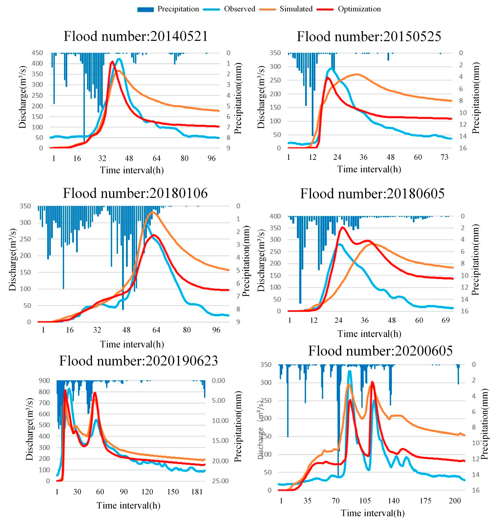
and Figure 10, after optimizing the parameters for the Mazhou watershed, the Nash–Sutcliffe efficiency coefficient for four out of six floods exceeded 0.75, the correlation coefficient surpassed 0.8, the relative errors of flood peaks were all constrained within 0.1, and the differences in the time of occurrence of flood peaks were all controlled within 2 h.

3.2. Effect of Different DEM Resolutions on Simulation Results

To study the effects of different DEM resolutions on flood simulation results, we selected nine floods from the Anhe (20130604, 20160716, 20210530), Dutou (20150525, 20160126, 20160826), and Mazhou watersheds (20140521, 20180106, 20190623). The original 90 m-resolution DEM was sequentially resampled to 150 m, 200 m, 300 m, 400 m, and 500 m, resulting in seven spatial resolution DEMs ranging from 30 m to 500 m used as input data for the Liuxihe model’s flood simulation. Notably, in the Dutou watershed, when the DEM resolution was resampled to 500 m, it was not possible to extract information about the river where the hydrological station at the watershed outlet was located. Therefore, the highest resolution used for the Dutou watershed was 400 m. Figure 11 illustrates the changes in flood modeling accuracy across different DEM resolutions.

For the Anhe watershed: a. The simulation results show that as the DEM resolution goes from 30 m to 500 m, the flood simulation accuracy as a whole gradually decreases, which is manifested in the gradual decrease in the coefficient of certainty and the correlation coefficient, the gradual increase in the process relative error and the relative error of the peak, and the peak present time error also gradually increases. b. It can be found that the coefficient of certainty decreases sharply in the interval from 200 m to 300 m. The certainty coefficient of 20130604 drops from 0.908 to 0.76, the certainty coefficient of 20160716 drops from 0.505 to 0.23, and the certainty coefficient of 20210530 drops from 0.437 to 0.076.

For the Dutou watershed: a. The simulation results show that as the DEM resolution increases from 30 m to 500 m, the accuracy of the flood simulation becomes lower and lower, which is manifested in the fact that the coefficient of determinism and correlation coefficient are a gradually decreasing trend, the process relative error and the relative error of flood flow are gradually increasing, and the peak-appearance time error is growing bigger and bigger. b. It can be seen that from the resolution of 200 m to the resolution of 300 m for 20150525, 20160126, and 20160826, the coefficient of certainty decreases from 0.867 to 0.799, 0.725 to 0.671, and 0.777 to 0.693, respectively, and all of these plummeted relative to the 30–200 m resolution.

For the Mazhou watershed: a. The simulation results show that with the gradual increase in DEM resolution (30 m to 500 m), the accuracy of flood simulation gradually decreases, which is reflected in the gradual decrease in the coefficient of determinism and correlation coefficient. The process relative error and the relative error of the flood flow become bigger and bigger, and the peak-appearance time error is gradually increasing. b. It can be seen that from the resolution of 400 m to the resolution of 500 m, Nash efficiency coefficients of 20140521, 20180106, and 20190623 decrease from −0.11 to −0.26, 0.288 to 0.24, and 0.618 to 0.541, respectively, and a sudden drop occurs relative to the 30–400 m resolution.

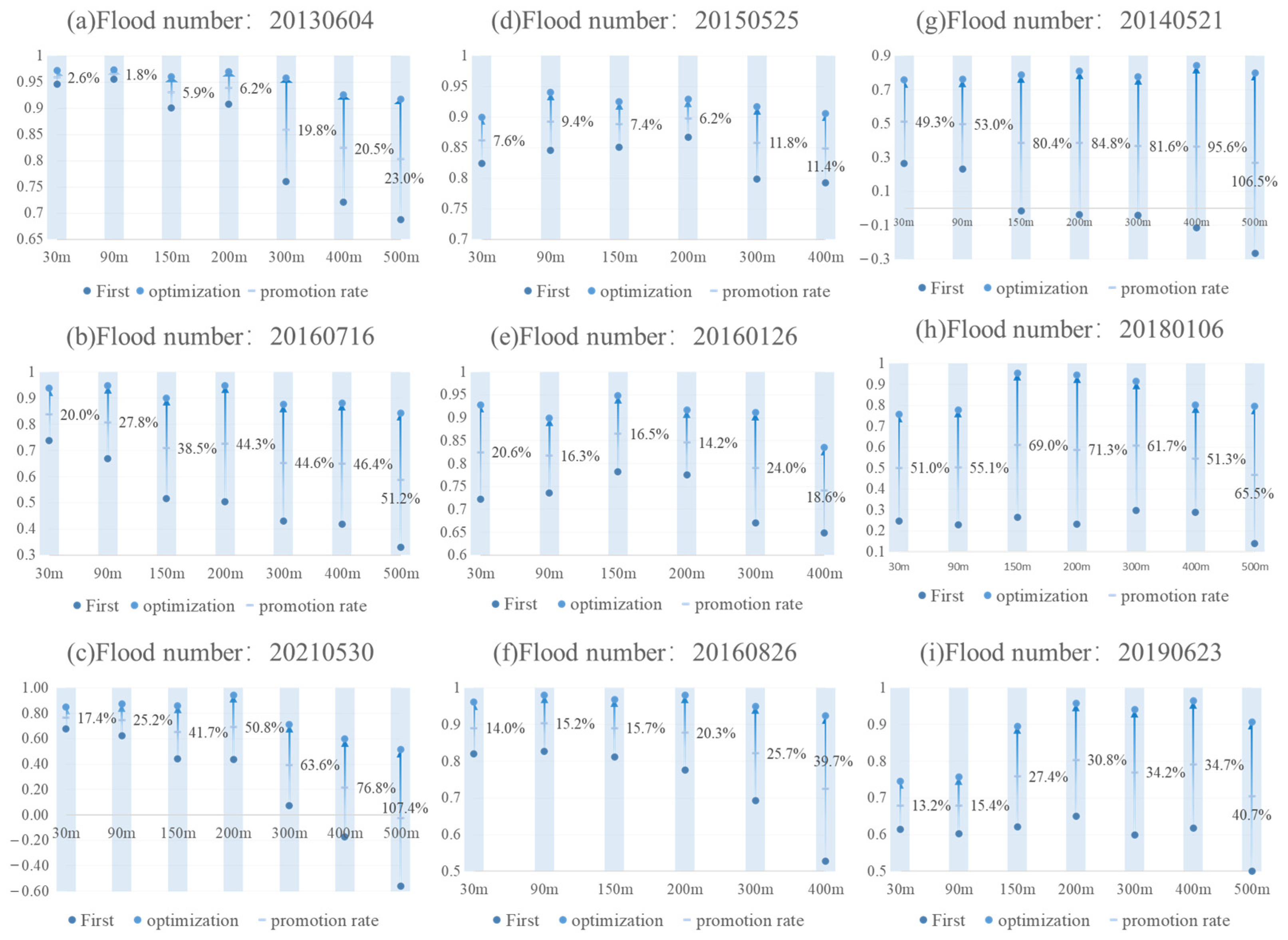
3.3. Spatial Scale Effects of Model Parameters at Different DEM Resolutions

In this section, we analyze the parameter preferences of the flood simulations at various DEM resolutions to observe the scaling effect on the optimal model parameters as resolution changes. As shown in the Figure 12, the simulation accuracy at 300 m, 400 m, and 500 m resolutions in the Anhe Watershed was significantly improved, especially for medium- and large-scale floods. For example, the Nash–Sutcliffe efficiency coefficients for the 20130604 (medium) and 20160716 (large) reached 0.918 and 0.843, respectively, at 500 m resolution. In contrast, the Nash–Sutcliffe efficiency coefficients for the 20210530 (small) were only 0.598 and 0.514 at 400 m and 500 m resolutions, respectively, indicating that these resolutions are not suitable for effective flood simulation of small-scale floods. The simulation accuracy at 300 m and 400 m resolutions showed significant improvement in the Dutou watershed, particularly for medium- and large-scale floods compared to small-scale floods. For instance, the Nash–Sutcliffe efficiency coefficients for the 20150525 (medium) and 20160826 (large) events increased to 0.906 and 0.924, respectively, at 400 m resolution, while the coefficient for the 20160126 (small) event only improved to 0.835. The simulation accuracy at 500 m resolution improved substantially in the Mazhou watershed, especially for medium- and large-volume floods. For example, the Nash–Sutcliffe efficiency coefficients for the 20140521 (medium) and 20190623 (large) events reached 0.901 and 0.908, respectively, while the coefficient for the 20180106 (small) event only improved to 0.795. These results indicate that while flood simulation accuracy is significantly enhanced after parameter optimization, there is still a decline in accuracy with increasing resolution. However, parameter optimization can effectively mitigate the reduction in simulation accuracy associated with higher DEM resolutions.

Due to space limitations, we use the Mazhou watershed as an example to demonstrate changes in the model’s optimal parameters at various resolutions, from 90 m to 500 m, for the 20140521, 20180106, and 20190623 floods after parameter optimization. The results indicate that some model parameters vary with resolution when achieving optimal simulation for the same flood event. Figure 13 illustrates that some model parameters change when achieving the best simulation results for the same flood event at different resolutions. This indicates a scale effect on parameter values, where parameters closely related to resolution, such as river bottom slope and river roughness, are more likely to vary. The range of parameter values varies with changes in DEM resolution, with variation intervals consistently between 0.5 and 1.5.

3.4. Statistics of the Surface Flow Production at Different DEM Resolutions

The results in Figure 14 indicated that the magnitude of flood production across different DEM resolutions is similar, and the statistical analysis of 60 flow production results showed an error range within ±10% for 59 and ±5% for 50.

4. Discussion

Understanding the impact of DEM resolution on flood simulation outcomes is critical for clarifying how varying DEM resolutions influence the accuracy of flood simulations. This insight assists hydrological agencies in selecting the most suitable DEM resolution for hydrological modeling in flood forecasting. By optimizing the DEM resolution, flood simulation accuracy can be maximized while minimizing computational costs. Achieving this balance ensures that the chosen DEM resolution is both cost-effective and meets required time constraints without sacrificing simulation accuracy. Therefore, identifying an optimal DEM resolution range that harmonizes simulation costs, time demands, and accuracy is crucial for effective and precise flood forecasting.

Our results complement, corroborate, and extend previous research findings: previous studies often divided resolution intervals into fine intervals within 90 m, conducting flood simulations using aggregate or semi-distributed hydrological models. These studies showed that while high-resolution simulations performed slightly better, there was not a significant difference in the overall flood process simulation within 90 m resolution [27], consistent with our findings. This agrees with the conclusion that flood simulation accuracy gradually decreases as resolution increases [28]. Our study extends the resolution range to 500 m at 100 m intervals, broadening the applicability of the results. Some researchers constructed hydrological models using DEM resolutions between 25 m and 1600 m. Their results indicated that flood peak simulation accuracy decreases slowly until a 200 m resolution, then drops significantly beyond 200 m [30]. These findings align with our conclusion that flood peak simulation accuracy sharply decreases between 200 m and 300 m resolutions. Furthermore, this interval may vary with the watershed scale.

As an important input data of the PBDHMs, a DEM can be found through the above study: the size of its resolution directly affects the flood simulation. In the following, we further investigate the reasons for the differences in the flood simulation effects of different DEM resolutions from the aspects of streamflow production and convergence.

(1)

Watershed Flow Analysis

The flow production calculation sub-module in the Liuxihe model computes flow production for each unit watershed by analyzing rainfall and evapotranspiration. This calculation is then categorized into surface runoff, loamy center flow, and subsurface runoff. The surface runoff calculation results, presented below, were derived from parameter-optimized flood process lines. The findings indicated that while varying DEM resolutions result in changes to model input data—such as soil, land use, and rainfall—the overall impact on flood simulation accuracy is minimal and is not the primary factor contributing to accuracy decline.

(2)

Watershed Confluence Analysis

The declining accuracy of flood simulations is likely attributable to issues in watershed convergence. Our investigation focuses on two primary aspects. First, the calculation of catchment channel confluence depends on the watershed’s water system, which encompasses basic characteristics such as shape, length, and direction. The accuracy of river channel confluence calculations improves when the extracted watershed water system closely aligns with the actual water system. Conversely, significant deviations in the extracted watershed water system’s grade and shape from the actual river channel information increase errors in confluence calculations. The water systems of the Anhe, Dutou, and Mazhou watersheds were extracted at different DEM resolutions up to the tertiary river network. The findings revealed that as DEM resolution increases, information about some upstream tributaries is gradually lost, leading to the disappearance of certain river sections and alterations in the water system’s direction, particularly in river bends. A 500 m resolution was not utilized for the Dutou watershed because river information at the hydrological station’s location could not be extracted, resulting in a significantly different extracted watershed range compared to the actual watershed range. This distortion in the extracted water system information increases errors in confluence calculations, thereby affecting the accuracy of flood simulations. Second, the slope factor, the first-order derivative of DEM, characterizes the intrinsic changes in DEM. Statistical analysis revealed that as DEM resolution increases, the average slope of the three watersheds decreases, which corresponds with the observation that flood simulation accuracy diminishes with higher resolution. When the resolution reaches 300 m, simulation accuracy decreases sharply, indicating a significant reduction in accuracy when the average slope falls below a certain threshold or the watershed attains a particular level of stability. For watersheds ranging from 500 km² to 2000 km², this threshold extends from 400 m to 500 m.

In this study, there are also deficiencies in the experimental process, such as the choice of resampling method and uncertainty concerning hydrological model parameters. On one hand, further research is needed on DEM data resampling methods. On the other hand, the next step of the study will involve a quantitative analysis of how resolution impacts flood simulation accuracy. These findings will have significant practical implications for selecting the optimal DEM resolution for flood simulation across different river watersheds.

5. Conclusions

This study utilized the Liuxihe model to simulate flood events in three watersheds located in Ganzhou, Jiangxi Province, China, to investigate the relationship between DEM resolution and flood simulation accuracy. The main findings are as follows.

(1) The Liuxihe model achieved high flood simulation accuracy across the three watersheds, particularly after parameter optimization, which significantly enhanced model performance and met the accuracy requirements for flood forecasting. (2) The accuracy exhibited a gradual decline from 30 m to 200 m resolution, followed by a sharp drop between 200 m and 300 m. This pattern was particularly evident in smaller watersheds with catchment areas of 500 km² or less, such as the Anhe and Dutou watersheds. In larger watersheds, like Mazhou, the threshold interval extended further, with the critical range reaching 400–500 m. (3) The optimization of Liuxihe model parameters effectively mitigated the decrease in flood simulation accuracy associated with coarser DEM resolutions, allowing for the maintenance of higher accuracy even at larger spatial scales. Different DEM resolutions for the same flood event necessitate varying optimal parameter combinations to achieve the best simulation results, with significant adjustments required for parameters such as riverbed slope and river roughness. (4) The impact of DEM resolution on simulation accuracy was analyzed from the perspectives of flow production and confluence, as follows. a. Although changes in DEM resolution influence model input data such as soil, land use, and rainfall, these factors have a minimal impact on surface flow production within the watershed and are not the primary contributors to changes in accuracy. b. The primary influence of increased DEM resolution lies in its effect on convergence mechanisms. Higher DEM resolution can misalign the extracted water system of the watershed, affecting river convergence calculations and thereby reducing flood simulation accuracy. Additionally, higher DEM resolution leads to a decrease in the average slope of the watershed, a phenomenon known as watershed flattening. When this flattening surpasses a certain threshold, a significant decline in flood simulation accuracy is observed.