
HA-Net for Bare Soil Extraction Using Optical Remote Sensing Images

Abstract
:1. Introduction
- The Hybrid Attention Network (HA-Net) is proposed in this paper, which possesses the excellent feature learning ability for bare soils, and effectively suppress the interference of the background, so excellent extraction performance for bare soil from remote sensing can be achieved.
- By introducing the attention mechanism, the Spatial Information Perception Module (SIPM) and Channel Information Enhancement Module (CIEM) are proposed, which can effectively learn multiscale information of the bare soil and better suppress the complex background noise.
- In the decoder, the Semantic Reconstructing-based Upsampling Module (SRUM) is constructed, which improves the ability of capturing the detailed information for bare soils during the downsampling process in the encoder.
- HA-Net not only enables high-precision automatic extraction of bare soil targets, but also has significant application values in the semantic segmentation for other typical targets in remote sensing images.
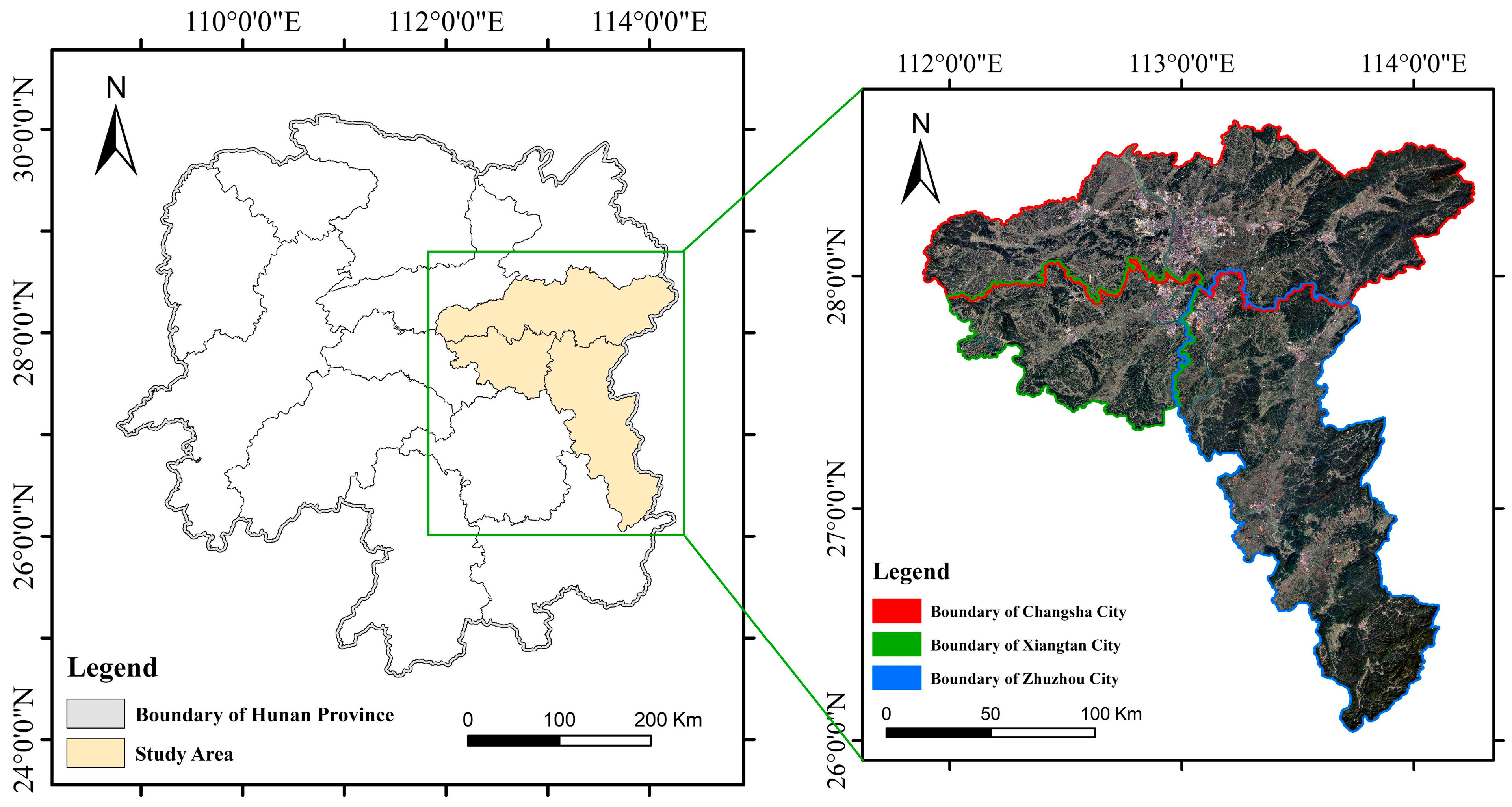
2. Study Regions and Data
2.1. Study Regions
2.2. CBERS-04A Data
2.3. Data Set
3. Methods
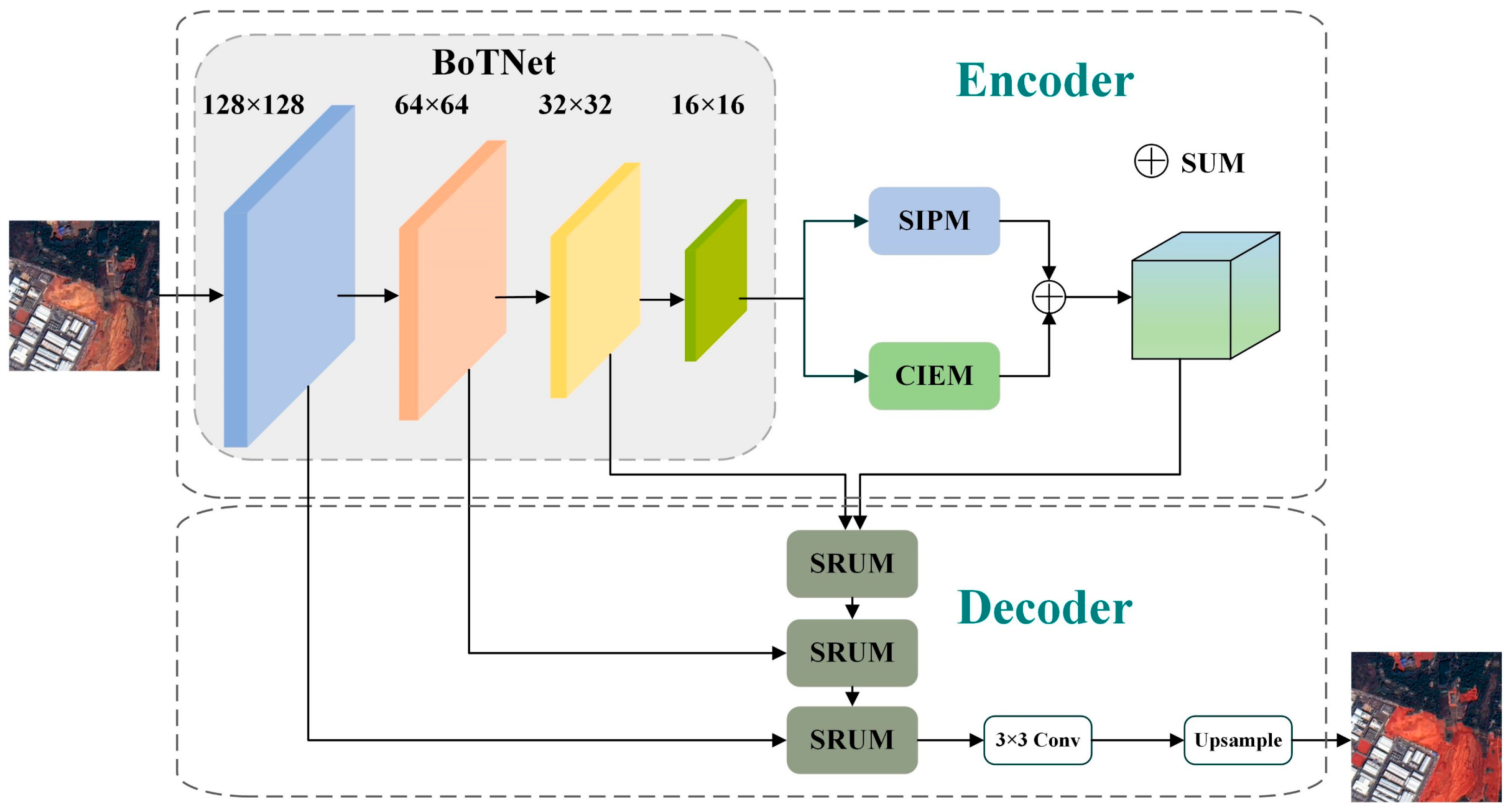
3.1. Overall Framework of HA-Net
3.2. The Encoder
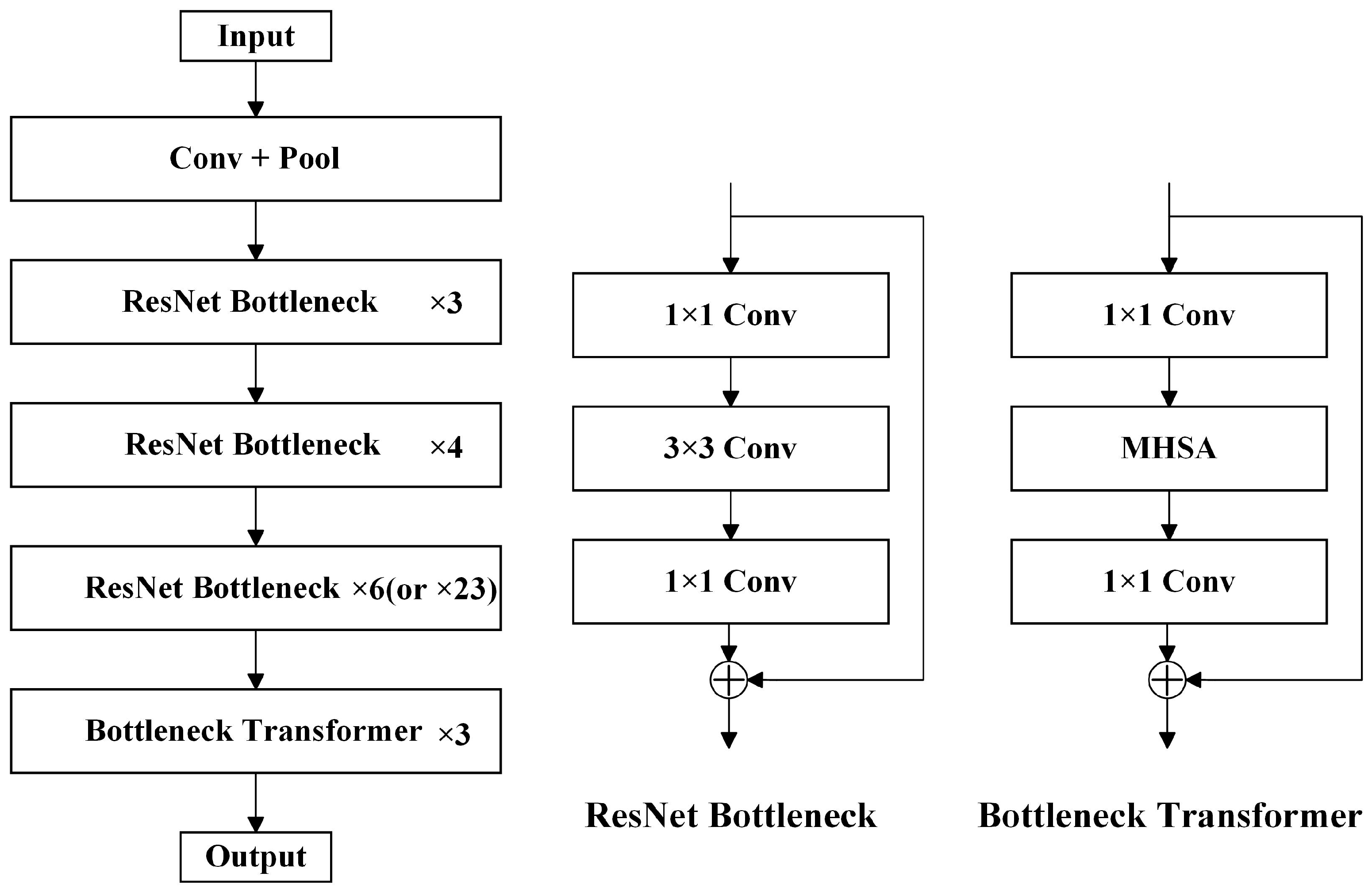
3.2.1. Backbone
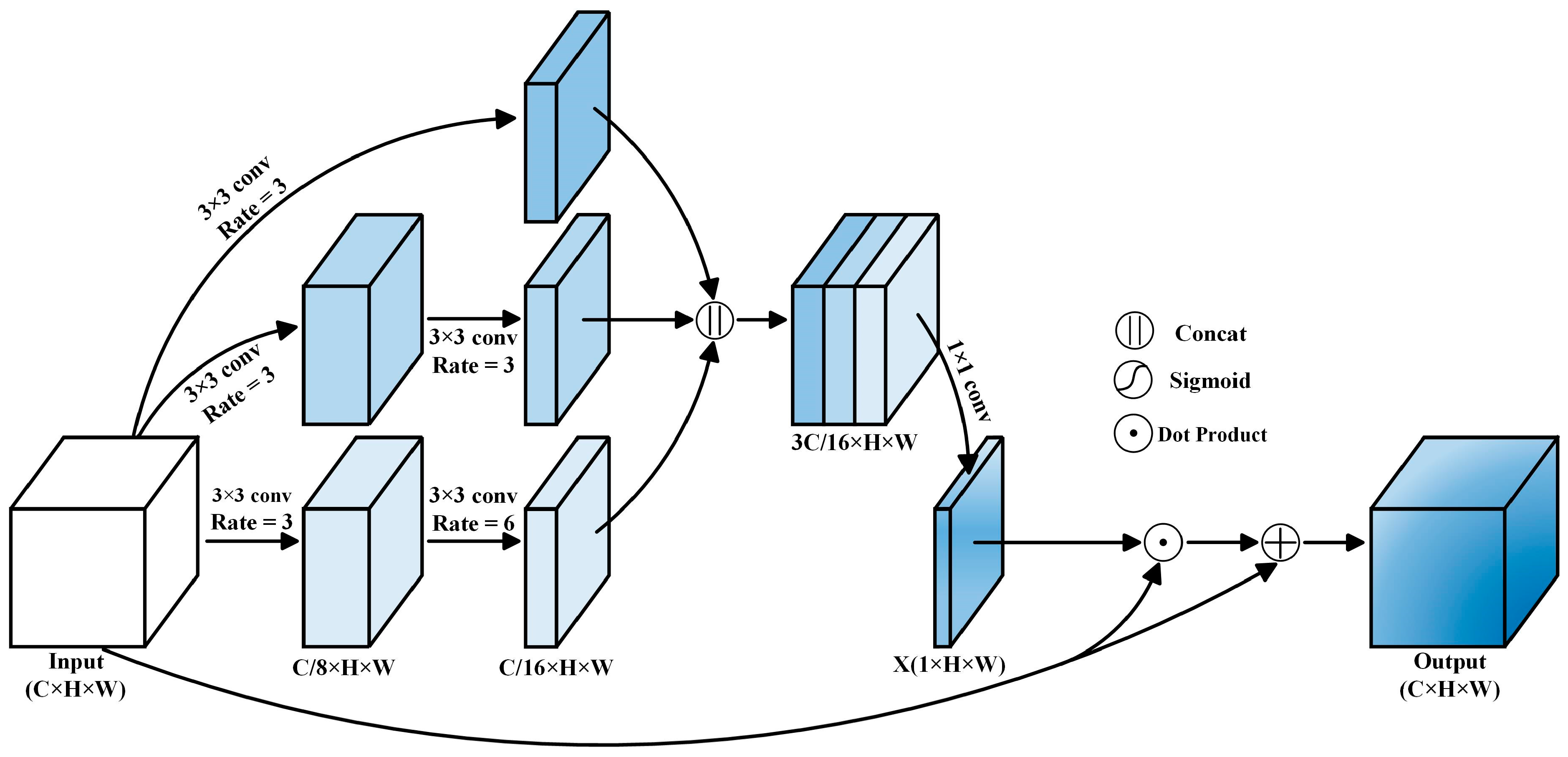
3.2.2. SIPM
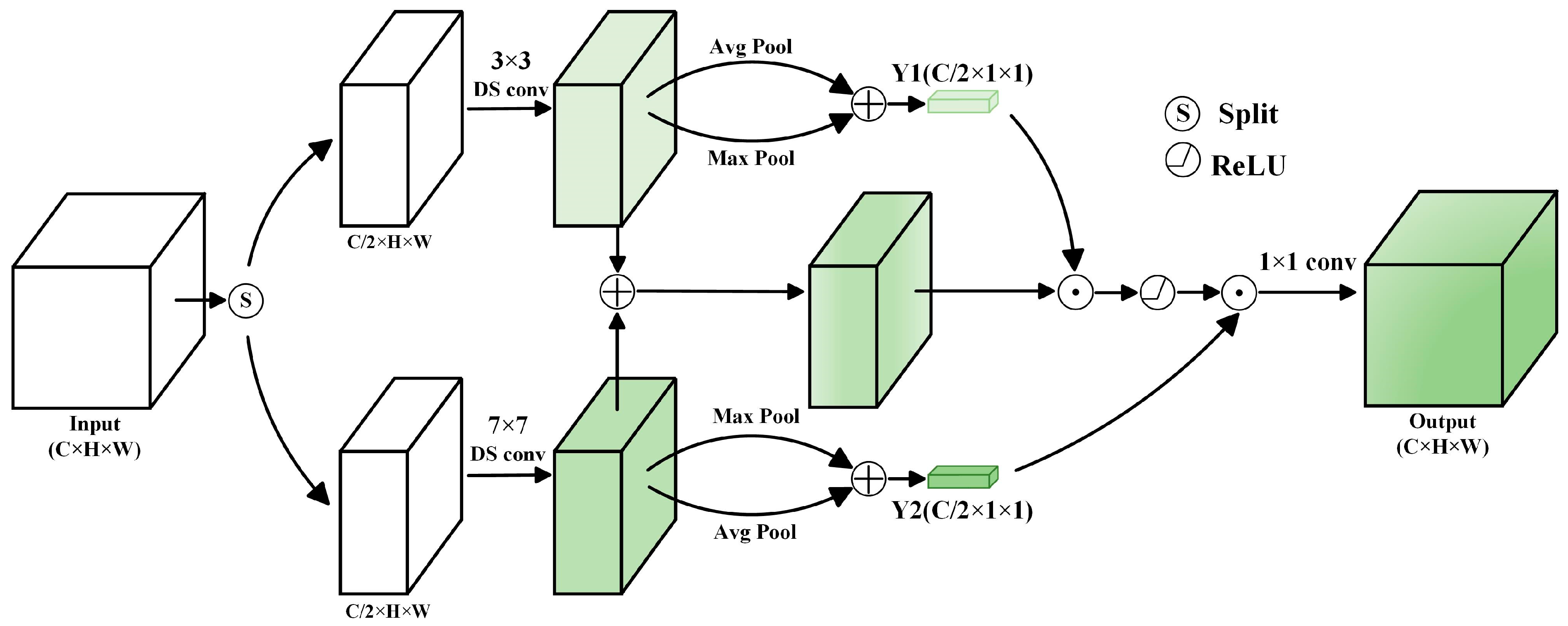
3.2.3. CIEM
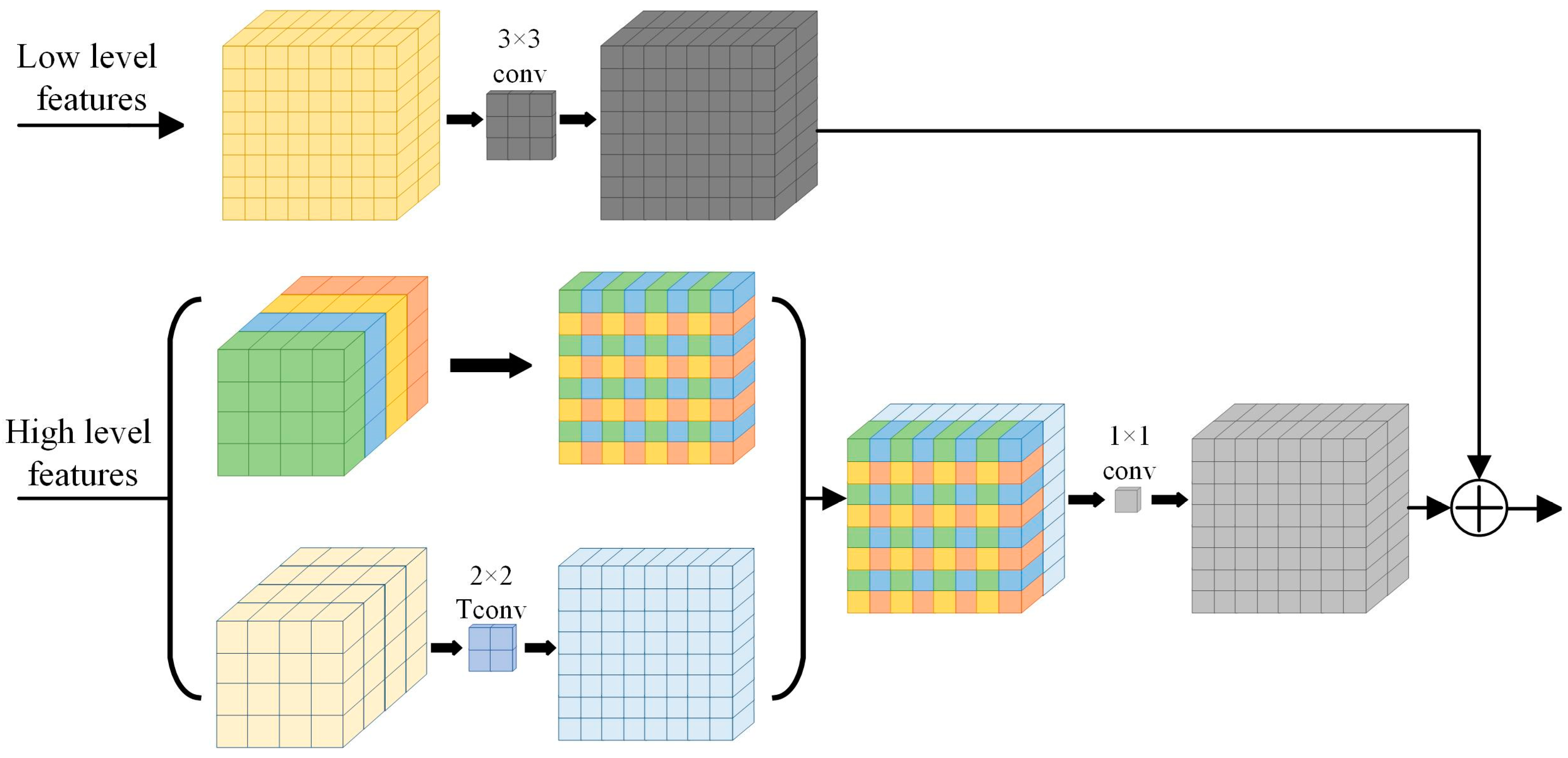
3.3. The Decoder
4. Experiments and Results
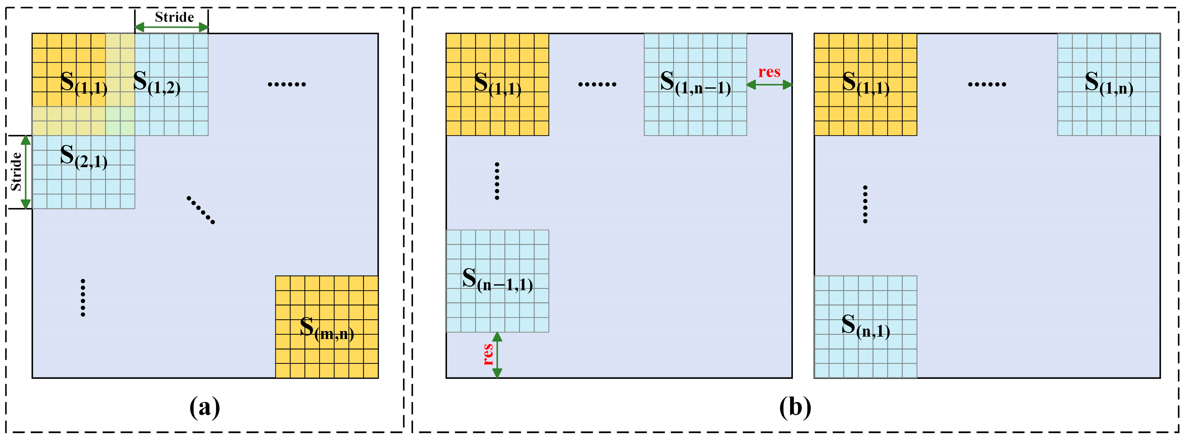
4.1. The Stitching Strategy of the Sliding Windows
4.2. Experimental Environment and Training Parameter Settings
4.3. Experimental Results and the Analysis
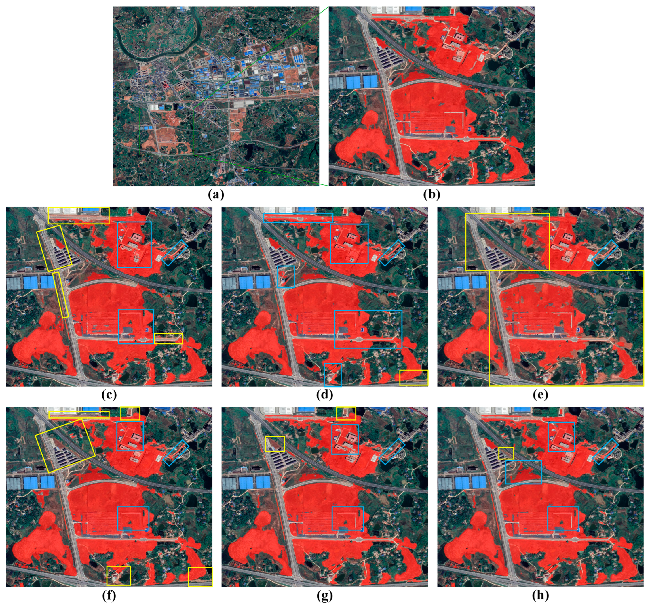
4.3.1. Bare Soil Extraction by Different Networks
4.3.2. Ablation Study
4.3.3. Generalization Ability Experiments
5. Discussion
6. Conclusions
Author Contributions
Funding
Data Availability Statement
Acknowledgments
Conflicts of Interest
References
- Ellis, E.; Pontius, R. Land-use and land-cover change. Encycl. Earth 2007, 1, 1–4. [Google Scholar]
- Lambin, E.F.; Turner, B.L.; Geist, H.J.; Agbola, S.B.; Angelsen, A.; Bruce, J.W.; Coomes, O.T.; Dirzo, R.; Fischer, G.; Folke, C.; et al. The causes of land-use and land-cover change: Moving beyond the myths. Glob. Environ. Chang. 2001, 11, 26–269. [Google Scholar] [CrossRef]
- Müller, H.; Griffiths, P.; Hostert, P. Long-term deforestation dynamics in the Brazilian Amazon—Uncovering historic frontier development along the Cuiabá–Santarém highway. Int. J. Appl. Earth Obs. 2016, 44, 61–69. [Google Scholar] [CrossRef]
- Xian, G.; Crane, M. An analysis of urban thermal characteristics and associated land cover in Tampa Bay and Las Vegas using Landsat satellite data. Remote Sens. Environ. 2006, 104, 147–156. [Google Scholar] [CrossRef]
- Silvero, N.E.Q.; Demattê, J.A.M.; Amorim, M.T.A.; dos Santos, N.V.; Rizzo, R.; Safanelli, J.L.; Poppiel, R.R.; de Sousa Mendes, W.; Bonfatti, B.R. Soil variability and quantification based on Sentinel-2 and Landsat-8 bare soil images: A comparison. Remote Sens. Environ. 2021, 252, 112117. [Google Scholar] [CrossRef]
- Wang, W.X.; Chai, F.H.; Ren, Z.H.; Wang, X.; Wang, S.; Li, H.; Gao, R.; Xue, L.; Peng, L.; Zhang, X.; et al. Process, achievements and experience of air pollution control in China since the founding of the People's Republic of China 70 years ago. Res. Environ. Sci. 2019, 32, 1621–1635. [Google Scholar]
- Wuepper, D.; Borrelli, P.; Finger, R. Countries and the global rate of soil erosion. Nat. Sustain. 2020, 3, 51–55. [Google Scholar] [CrossRef]
- Xu, H. Dynamics of Bare Soil in A Typical Reddish Soil Loss Region of Southern China: Changting County, Fujian Province. Sci. Geogr. Sin. 2013, 33, 489–496. [Google Scholar]
- Liang, S.; Fang, H.; Chen, M. Atmospheric correction of landsat ETM+ land surface imagery-Part I: Methods. IEEE Trans. Geosci. Remote Sens. 2001, 39, 2490–2498. [Google Scholar] [CrossRef]
- Pianalto, F.S.; Yool, S.R. Monitoring fugitive dust emission sources arising from construction: A remote-sensing approach. GIsci. Remote Sens. 2013, 50, 251–270. [Google Scholar] [CrossRef]
- Dou, P.; Chen, Y. Dynamic monitoring of land-use/land-cover change and urban expansion in shenzhen using landsat imagery from 1988 to 2015. Int. J. Remote Sens. 2017, 38, 5388–5407. [Google Scholar] [CrossRef]
- Zhang, Y.; Shen, W.; Li, M.; Lv, Y. Assessing spatio-temporal changes in forest cover and fragmentation under urban expansion in Nanjing, eastern China, from long-term Landsat observations (1987–2017). Appl. Geogr. 2020, 117, 102190. [Google Scholar] [CrossRef]
- Chai, B.; Li, P. Annual Urban Expansion Extraction and Spatio-Temporal Analysis Using Landsat Time Series Data: A Case Study of Tianjin. IEEE J. Sel. Top. Appl. Earth Obs. Remote Sens. 2018, 11, 2644–2656. [Google Scholar] [CrossRef]
- Schultz, M.; Clevers, J.G.P.W.; Carter, S.; Verbesselt, J.; Avitabile, V.; Quang, H.V.; Herold, M. Performance of vegetation indices from Landsat time series in deforestation monitoring. Int. J. Appl. Earth Obs. Geoinf. 2016, 52, 318–327. [Google Scholar] [CrossRef]
- Hamunyela, E.; Verbesselt, J.; Herold, M. Using spatial context to improve early detection of deforestation from Landsat time series. Remote Sens. Environ. 2016, 172, 126–138. [Google Scholar] [CrossRef]
- Pendrill, F.; Gardner, T.A.; Meyfroidt, P.; Persson, U.M.; Adams, J.; Azevedo, T.; Bastos Lima, M.G.; Baumann, M.; Curtis, P.G.; Sy, V.D.; et al. Disentangling the numbers behind agriculture-driven tropical deforestation. Science 2022, 377, eabm9267. [Google Scholar] [CrossRef]
- Zhu, F.; Wang, H.; Li, M.; Diao, J.; Shen, W.; Zhang, Y.; Wu, H. Characterizing the effects of climate change on short-term post-disturbance forest recovery in southern China from Landsat time-series observations (1988–2016). Front. Earth Sci. 2020, 14, 816–827. [Google Scholar] [CrossRef]
- Mo, Y.; Kearney, M.S.; Turner, R.E. Feedback of coastal marshes to climate change: Long-term phenological shifts. Ecol. Evol. 2019, 9, 6785–6797. [Google Scholar] [CrossRef]
- Rikimaru, A.; Roy, P.S.; Miyatake, S. Tropical forest cover density mapping. Trop. Ecol. 2002, 43, 39–47. [Google Scholar]
- Li, S.; Chen, X. A new bare-soil index for rapid mapping developing areas using landsat 8 data. ISPRS Arch. 2014, 40, 139–144. [Google Scholar] [CrossRef]
- Nguyen, C.T.; Chidthaisong, A.; Kieu Diem, P.; Huo, L.Z. A modified bare soil index to identify bare land features during agricultural fallow-period in southeast Asia using Landsat 8. Land 2021, 10, 231. [Google Scholar] [CrossRef]
- Rasul, A.; Balzter, H.; Ibrahim, G.R.F.; Hameed, H.M.; Wheeler, J.; Adamu, B.; Ibrahim, S.; Najmaddin, P.M. Applying Built-Up and Bare-Soil Indices from Landsat 8 to Cities in Dry Climates. Land 2018, 7, 81. [Google Scholar] [CrossRef]
- Chen, L.; Cai, X.; Xing, J.; Li, Z.; Zhu, W.; Yuan, Z.; Fang, Z. Towards transparent deep learning for surface water detection from SAR imagery. Int. J. Appl. Earth Obs. Geoinf. 2023, 118, 103287. [Google Scholar] [CrossRef]
- Chen, L.; Zhang, P.; Xing, J.; Li, Z.; Xing, X.; Yuan, Z. A multi-scale deep neural network for water detection from SAR images in the mountainous areas. Remote Sens. 2020, 12, 3205. [Google Scholar] [CrossRef]
- Chen, L.; Weng, T.; Xing, J.; Li, Z.; Yuan, Z.; Pan, Z.; Tan, S.; Luo, R. Employing deep learning for automatic river bridge detection from SAR images based on adaptively effective feature fusion. Int. J. Appl. Earth Obs. Geoinf. 2021, 102, 102425. [Google Scholar] [CrossRef]
- Vaswani, A.; Shazeer, N.; Parmar, N.; Uszkoreit, J.; Jones, L.; Gomez, A.N.; Kaiser, L. Attention is all you need. In Proceedings of the Advances in Neural Information Processing Systems 30 (NIPS 2017), Long Beach, CA, USA, 4–9 December 2017. [Google Scholar]
- Chen, J.; Yi, J.; Chen, A.; Lin, H. SRCBTFusion-Net: An Efficient Fusion Architecture via Stacked Residual Convolution Blocks and Transformer for Remote Sensing Image Semantic Segmentation. IEEE Trans. Geosci. Remote Sens. 2023, 61, 1–16. [Google Scholar] [CrossRef]
- Zhao, H.; Chen, X. Use of normalized difference bareness index in quickly mapping bare areas from TM/ETM+. In Proceedings of the International Geoscience and Remote Sensing Symposium, Seoul, Republic of Korea, 29 July 2005. [Google Scholar]
- Cheng, G.; Yuan, X.; Yao, X.; Yan, K.; Zeng, Q.; Xie, X.; Han, J. Towards large-scale small object detection: Survey and benchmarks. IEEE Trans. Pattern Anal. Mach. Intell. 2023, 45, 13467–13488. [Google Scholar] [CrossRef]
- Deng, Y.; Wu, C.; Li, M.; Chen, R. RNDSI: A ratio normalized difference soil index for remote sensing of urban/suburban environments. Int. J. Appl. Earth Obs. Geoinf. 2015, 39, 40–48. [Google Scholar] [CrossRef]
- He, C.; Liu, Y.; Wang, D.; Liu, S.; Yu, L.; Ren, Y. Automatic extraction of bare soil land from high-resolution remote sensing images based on semantic segmentation with deep learning. Remote Sens. 2023, 15, 1646. [Google Scholar] [CrossRef]
- Liu, D.; Chen, N. Satellite monitoring of urban land change in the middle Yangtze River Basin urban agglomeration, China between 2000 and 2016. Remote Sens. 2017, 9, 1086. [Google Scholar] [CrossRef]
- Jesus, G.T.; Itami, S.N.; Segantine, T.Y.F.; Junior, M.F.C. Innovation path and contingencies in the China-Brazil Earth Resources Satellite program. Acta Astronaut. 2021, 178, 382–391. [Google Scholar] [CrossRef]
- Cai, X.; Chen, L.; Xing, J.; Xing, X.; Luo, R.; Tan, S.; Wang, J. Automatic extraction of layover from InSAR imagery based on multilayer feature fusion attention mechanism. IEEE Geosci. Remote Sens. Lett. 2021, 19, 1–5. [Google Scholar] [CrossRef]
- Srinivas, A.; Lin, T.Y.; Parmar, N.; Shlens, J.; Abbeel, P.; Vaswani, A. Bottleneck transformers for visual recognition. In Proceedings of the IEEE/CVF Conference on Computer Vision and Pattern Recognition, Nashville, TN, USA, 20–25 June 2021. [Google Scholar]
- He, K.; Zhang, X.; Ren, S.; Sun, J. Deep residual learning for image recognition. In Proceedings of the IEEE Conference on Computer Vision and Pattern Recognition, Las Vegas, NV, USA, 27–30 June 2016. [Google Scholar]
- Chen, L.; Cai, X.; Li, Z.; Xing, J.; Ai, J. Where is my attention? An explainable AI exploration in water detection from SAR imagery. Int. J. Appl. Earth Obs. Geoinf. 2024, 130, 103878. [Google Scholar] [CrossRef]
- Zhang, Q.L.; Yang, Y.B. Sa-net: Shuffle attention for deep convolutional neural networks. In Proceedings of the ICASSP 2021-2021 IEEE International Conference on Acoustics, Speech and Signal Processing (ICASSP), Toronto, ON, Canada, 6–11 June 2021. [Google Scholar]
- Daubechies, I.; DeVore, R.; Foucart, S.; Hanin, B.; Petrova, G. Nonlinear approximation and (deep) ReLU networks. Constr. Approx. 2022, 55, 127–172. [Google Scholar] [CrossRef]
- Chen, L.C.; Zhu, Y.; Papandreou, G.; Schroff, F.; Adam, H. Encoder-decoder with atrous separable convolution for semantic image segmentation. In Proceedings of the European Conference on Computer Vision (ECCV), Munich, Germany, 8–14 September 2018. [Google Scholar]
- Fu, J.; Liu, J.; Tian, H.; Li, Y.; Bao, Y.; Fang, Z.; Lu, H. Dual attention network for scene segmentation. In Proceedings of the IEEE/CVF Conference on Computer Vision and Pattern Recognition, Long Beach, CA, USA, 15–21 June 2019. [Google Scholar]
- Wang, L.; Fang, S.; Meng, X.; Li, R. Building extraction with vision transformer. IEEE Trans. Geosci. Remote Sens. 2022, 60, 1–11. [Google Scholar] [CrossRef]
- Hu, J.; Huang, L.; Ren, T.; Zhang, S.; Ji, R.; Cao, L. You only segment once: Towards real-time panoptic segmentation. In Proceedings of the IEEE/CVF Conference on Computer Vision and Pattern Recognition, Vancouver, BC, Canada, 18–22 June 2023. [Google Scholar]
- Tong, X.Y.; Lu, Q.; Xia, G.S.; Zhang, L. Large-scale land cover classification in Gaofen-2 satellite imagery. In Proceedings of the IGARSS 2018-2018 IEEE International Geoscience and Remote Sensing Symposium, Valencia, Spain, 22–27 July 2018. [Google Scholar]


| Payload | Spectral Band | Spectral Range (μm) | Spatial Resolution (m) | Swath Width (km) | Revisit Cycle (Days) |
|---|---|---|---|---|---|
| WPM | 1 | 0.45 μm~0.9 μm | 2 | 90 | 31 |
| 2 | 0.45 μm~0.52 μm | 8 | |||
| 3 | 0.52 μm~0.59 μm | ||||
| 4 | 0.63 μm~0.69 μm | ||||
| 5 | 0.77 μm~0.89 μm | ||||
| MUX | 6 | 0.45 μm~0.52 μm | 17 | 90 | 31 |
| 7 | 0.52 μm~0.59 μm | ||||
| 8 | 0.63 μm~0.69 μm | ||||
| 9 | 0.77 μm~0.89 μm | ||||
| WFI | 10 | 0.45 μm~0.52 μm | 60 | 685 | 5 |
| 11 | 0.52 μm~0.59 μm | ||||
| 12 | 0.63 μm~0.69 μm | ||||
| 13 | 0.77 μm~0.89 μm |
| Input (16, 16, 2048) | ||
|---|---|---|
| Layer | Parameters | Output Shape |
| Branch-1 Conv2D | Filters = 256, Kernel_size = 3, Padding = 3, Dilation = 3 | (16, 16, 128) |
| Branch-2 Conv2D | Filters = 256, Kernel_size = 3, Padding = 3, Dilation = 3 | (16, 16, 256) |
| Branch-2 Conv2D | Filters = 128, Kernel_size = 3, Padding = 3, Dilation = 3 | (16, 16, 128) |
| Branch-3 Conv2D | Filters = 256, Kernel_size = 3, Padding = 3, Dilation = 3 | (16, 16, 256) |
| Branch-3 Conv2D | Filters = 128, Kernel_size = 3, Padding = 6, Dilation = 6 | (16, 16, 128) |
| Concat | None | (16, 16, 384) |
| Conv2D | Filters = 1, Kernel_size = 1, Padding = 0, Dilation = 1 | (16, 16, 1) |
| Sigmoid | None | (16, 16, 1) |
| Dot Product and SUM | None | (16, 16, 2048) |
| Input (16, 16, 2048) | ||
|---|---|---|
| Layer | Parameters | Output Shape |
| Split | None | (16, 16, 1024) × 2 |
| Depthwise Separable Conv2D 1 | Filters = 1024, Kernel_size = 3, Padding = 1, Dilation = 1 Filters = 1024, Kernel_size = 1, Padding = 0, Dilation = 1 | (16, 16, 1024) |
| Depthwise Separable Conv2D 1 | Filters = 1024, Kernel_size = 7, Padding = 3, Dilation = 1 Filters = 1024, Kernel_size = 1, Padding = 0, Dilation = 1 | (16, 16, 1024) |
| SUM | None | (16, 16, 1024) |
| Avg Pool × 2 | Kernel_size = 16 | (1, 1, 1024) × 2 |
| Max Pool × 2 | Kernel_size = 16 | (1, 1, 1024) × 2 |
| Sigmoid × 2 | None | (1, 1, 1024) × 2 |
| Dot Product | None | (16, 16, 1024) |
| ReLU | None | (16, 16, 1024) |
| Dot Product | None | (16, 16, 1024) |
| Conv2D | Filters = 2048, Kernel_size = 1, Padding = 0, Dilation = 1 | (16, 16, 2048) |
| Input [(N, N, C) and (2N, 2N, C/2)] 1 | |||
|---|---|---|---|
| Feature | Layer | Parameters | Output Shape |
| High-level Features | Pixel rearrangement | Upsampling factor = 2 | (2N, 2N, C/4) |
| Transposed Conv2D | Filters = C/4, Kernel_size = 2, Stride = 2, Padding = 0, Dilation = 1 | (2N, 2N, C/4) | |
| Concat | None | (2N, 2N, C/2) | |
| Conv2D | Filters = C/2, Kernel_size = 1, Padding = 0, Dilation = 1 | (2N, 2N, C/2) | |
| Low-level Features | Conv2D | Filters = C/2, Kernel_size = 3, Padding = 1, Dilation = 1 | (2N, 2N, C/2) |
| SUM | None | (2N, 2N, C/2) | |
| Layer | Parameters |
|---|---|
| Frame | PyTorch 1.20 |
| Language | Python 3.7 |
| CPU | Inter Xeon Silver 4210 |
| GPU (Single) | NVIDIA RTX 3090 |
| Predicted Values | |||
|---|---|---|---|
| Bare Soil | Non-Bare Soil | ||
| GroundTruth | Bare Soil | TP | FN |
| Non-Bare Soil | FP | TN | |
| Scene | Method | CPA (%) | IoU (%) | Recall (%) | F1 (%) |
|---|---|---|---|---|---|
| Scene I | DeepLabV3+ | 89.716 | 75.628 | 82.807 | 86.123 |
| DA-Net | 89.196 | 74.780 | 82.228 | 85.570 | |
| BuildFormer | 92.784 | 74.572 | 79.163 | 85.434 | |
| YOSO | 90.879 | 77.118 | 83.587 | 87.081 | |
| HA-Net-B50 | 92.216 | 81.423 | 87.432 | 89.760 | |
| HA-Net-B101 | 92.595 | 81.833 | 87.564 | 90.009 | |
| Scene II | DeepLabV3+ | 85.412 | 73.351 | 83.856 | 84.627 |
| DA-Net | 86.240 | 73.743 | 83.577 | 84.887 | |
| BuildFormer | 87.463 | 74.683 | 83.635 | 85.507 | |
| YOSO | 87.315 | 75.171 | 84.386 | 85.826 | |
| HA-Net-B50 | 88.689 | 78.680 | 87.455 | 88.068 | |
| HA-Net-B101 | 89.178 | 79.969 | 88.564 | 88.870 | |
| Average for Two Scenes | DeepLabV3+ | 87.564 | 74.490 | 83.332 | 85.375 |
| DA-Net | 87.718 | 74.262 | 82.903 | 85.229 | |
| BuildFormer | 90.124 | 74.628 | 81.399 | 85.471 | |
| YOSO | 89.097 | 76.145 | 83.987 | 86.454 | |
| HA-Net-B50 | 90.453 | 80.052 | 87.444 | 88.914 | |
| HA-Net-B101 | 90.887 | 80.901 | 88.064 | 89.440 |
| Backbone | Module-1 | Module-2 | CPA (%) | IoU (%) | Recall (%) | F1 (%) | |
|---|---|---|---|---|---|---|---|
| Average for Two Scenes | BoTNet50 | None | None | 87.261 | 74.562 | 83.696 | 85.427 |
| BoTNet101 | None | None | 87.753 | 75.233 | 84.087 | 85.866 | |
| BoTNet50 | SIPM | None | 88.785 | 77.256 | 85.642 | 87.167 | |
| BoTNet101 | SIPM | None | 89.210 | 78.018 | 86.167 | 87.648 | |
| BoTNet50 | CIEM | None | 88.478 | 76.774 | 85.341 | 86.858 | |
| BoTNet101 | CIEM | None | 88.762 | 77.478 | 85.926 | 87.305 | |
| BoTNet50 | SRUM | None | 87.694 | 75.327 | 84.261 | 85.927 | |
| BoTNet101 | SRUM | None | 88.200 | 76.150 | 84.825 | 86.460 | |
| BoTNet50 | SIPM | CIEM | 89.547 | 78.691 | 86.658 | 88.070 | |
| BoTNet101 | SIPM | CIEM | 89.729 | 79.189 | 87.090 | 88.383 |
| Method | CPA (%) | IoU (%) | Recall (%) | F1 (%) |
|---|---|---|---|---|
| DeepLabV3+ | 88.570 | 80.909 | 90.341 | 89.447 |
| DA-Net | 86.174 | 80.371 | 92.270 | 89.118 |
| BuildFormer | 92.579 | 73.352 | 77.935 | 84.628 |
| YOSO | 89.437 | 81.933 | 90.711 | 90.069 |
| HA-Net-B50 | 92.851 | 85.744 | 91.804 | 92.325 |
| HA-Net-B101 | 92.116 | 86.478 | 93.391 | 92.749 |
Disclaimer/Publisher’s Note: The statements, opinions and data contained in all publications are solely those of the individual author(s) and contributor(s) and not of MDPI and/or the editor(s). MDPI and/or the editor(s) disclaim responsibility for any injury to people or property resulting from any ideas, methods, instructions or products referred to in the content. |
© 2024 by the authors. Licensee MDPI, Basel, Switzerland. This article is an open access article distributed under the terms and conditions of the Creative Commons Attribution (CC BY) license (https://creativecommons.org/licenses/by/4.0/).
Share and Cite
Zhao, J.; Du, D.; Chen, L.; Liang, X.; Chen, H.; Jin, Y. HA-Net for Bare Soil Extraction Using Optical Remote Sensing Images. Remote Sens. 2024, 16, 3088. https://doi.org/10.3390/rs16163088
Zhao J, Du D, Chen L, Liang X, Chen H, Jin Y. HA-Net for Bare Soil Extraction Using Optical Remote Sensing Images. Remote Sensing. 2024; 16(16):3088. https://doi.org/10.3390/rs16163088
Chicago/Turabian StyleZhao, Junqi, Dongsheng Du, Lifu Chen, Xiujuan Liang, Haoda Chen, and Yuchen Jin. 2024. "HA-Net for Bare Soil Extraction Using Optical Remote Sensing Images" Remote Sensing 16, no. 16: 3088. https://doi.org/10.3390/rs16163088
APA StyleZhao, J., Du, D., Chen, L., Liang, X., Chen, H., & Jin, Y. (2024). HA-Net for Bare Soil Extraction Using Optical Remote Sensing Images. Remote Sensing, 16(16), 3088. https://doi.org/10.3390/rs16163088