Comparative Analysis of Satellite-Based Precipitation Data across the CONUS and Hawaii: Identifying Optimal Satellite Performance

Abstract

Accurate precipitation estimates are crucial for various hydrological and environmental applications. This study presents a comprehensive evaluation of three widely used satellite-based precipitation datasets (SPDs)—PERSIANN, CHIRPS, and MERRA—and a monthly reanalysis dataset—TERRA—that include data from across the contiguous United States (CONUS) and Hawaii, at daily, monthly, and yearly timescales. We present the performance of these SPDs using ground-based observations maintained by the USGS (United States Geological Survey). We employ evaluation metrics, such as the coefficient of determination (R²), root mean square error (RMSE), mean square error (MSE), and mean absolute error (MAE), to identify optimal SPDs. Our findings reveal that MERRA outperforms PERSIANN and CHIRPS on a daily scale, while CHIRPS is the best-performing dataset on a monthly scale. However, all datasets show limitations in accurately estimating absolute amount of precipitation totals. The spatial analysis highlights regional variations in the datasets’ performance, with MERRA consistently performing well across most regions, while CHIRPS and PERSIANN show strengths in specific areas and months. We also observe a consistent seasonal pattern in the performance of all datasets. This study contributes to the growing body of knowledge on satellite precipitation estimates and their applications, guiding the selection of suitable datasets based on the required temporal resolution and regional context. As such SPDs continue to evolve, ongoing evaluation and improvement efforts are crucial to enhance their reliability and support informed decision-making in various fields, including water resource management, agricultural planning, and climate studies.

1. Introduction

Precipitation, a fundamental component of the hydrological cycle, plays a pivotal role in shaping Earth’s climate and ecosystems [1,2,3]. The accurate measurement and monitoring of precipitation patterns and variability are important for a wide array of applications, ranging from water resources management and flood/drought forecasting to agricultural planning, climate change impact assessment, and ecosystem modeling [4,5,6]. Sub-daily and daily precipitation data are often used for hydrologic-hydrological modeling, to simulate streamflow and sediment load, to predict flood events, and to assess the impact of land-use changes on water resources [7,8]. Additionally, high temporal resolution precipitation data are particularly important for analyzing extreme events which can have significant impacts on ecosystems, agriculture, and human society [9,10,11], whereas monthly and seasonal precipitation estimates are equally valuable for long-term water resource planning, such as reservoir operations, water supply management, and drought monitoring [9,12]. These monthly to seasonal precipitation estimates are essential for understanding long-term climate variability, detecting trends, and evaluating the performance of climate models [11,13,14].

Accurate precipitation estimates at different temporal and spatial scales are valuable for developing, validating, and improving several numerical models, including climate models that project likely future changes [15,16]. While ground-based rain gauge networks have traditionally been the primary source of precipitation data, their spatial coverage is often limited, particularly in remote or topographically complex regions [4,17]. Consequently, satellite-based precipitation estimation techniques have emerged as an indispensable tool for providing spatially continuous and near-real-time precipitation data on a global scale [4,18,19]. These techniques have undergone significant advancements over the past few decades, driven by improvements in remote-sensing technologies and data-processing algorithms [4,20]. The diversity of satellite-based precipitation datasets (SPDs) has opened new opportunities for hydrological and meteorological applications, but it also raises critical questions regarding the accuracy, bias, and uncertainty associated with these products, particularly at the regional and local scales [21,22,23,24].

One of the major challenges in evaluating the performance of SPDs is the lack of a universal “ground truth” dataset for comparison [25,26]. Furthermore, the performance of SPDs can vary significantly depending on factors such as the topography, land cover, climate regimes, and underlying retrieval algorithms used [27,28]. While numerous studies have been conducted to assess the accuracy of SPDs, most of these efforts have focused on specific regions, a specific satellite, or limited time periods [24,29,30,31], making it challenging to draw comprehensive conclusions about their performance across broader spatial and temporal scales using different satellite estimates [28,32]. Notably, there is limited research that systematically evaluates and compares the performance of multiple SPDs across diverse geographic regions, spanning different topographic, land cover, and climatic conditions and using a robust and extensive ground-based observation network as the reference [32,33,34].

This research aims to fill this critical gap by conducting a comprehensive and systematic comparative analysis of SPDs against in-situ observations across a wide range of geographic regions, encompassing various environmental conditions. The overarching goal of this research is to identify the optimal SPDs for different geographic regions, considering spatial variations in performance across diverse topographic, land cover, and climatic conditions. This study proposes a methodological framework that provides a basis for selecting appropriate SPDs and offers valuable insights and recommendations for their hydrological and meteorological applications. This study contributes to the ongoing efforts to improve the accuracy and reliability of precipitation estimates, ultimately enhancing our understanding and management of water resources on a global scale.

2. Study Area, Materials and Methods

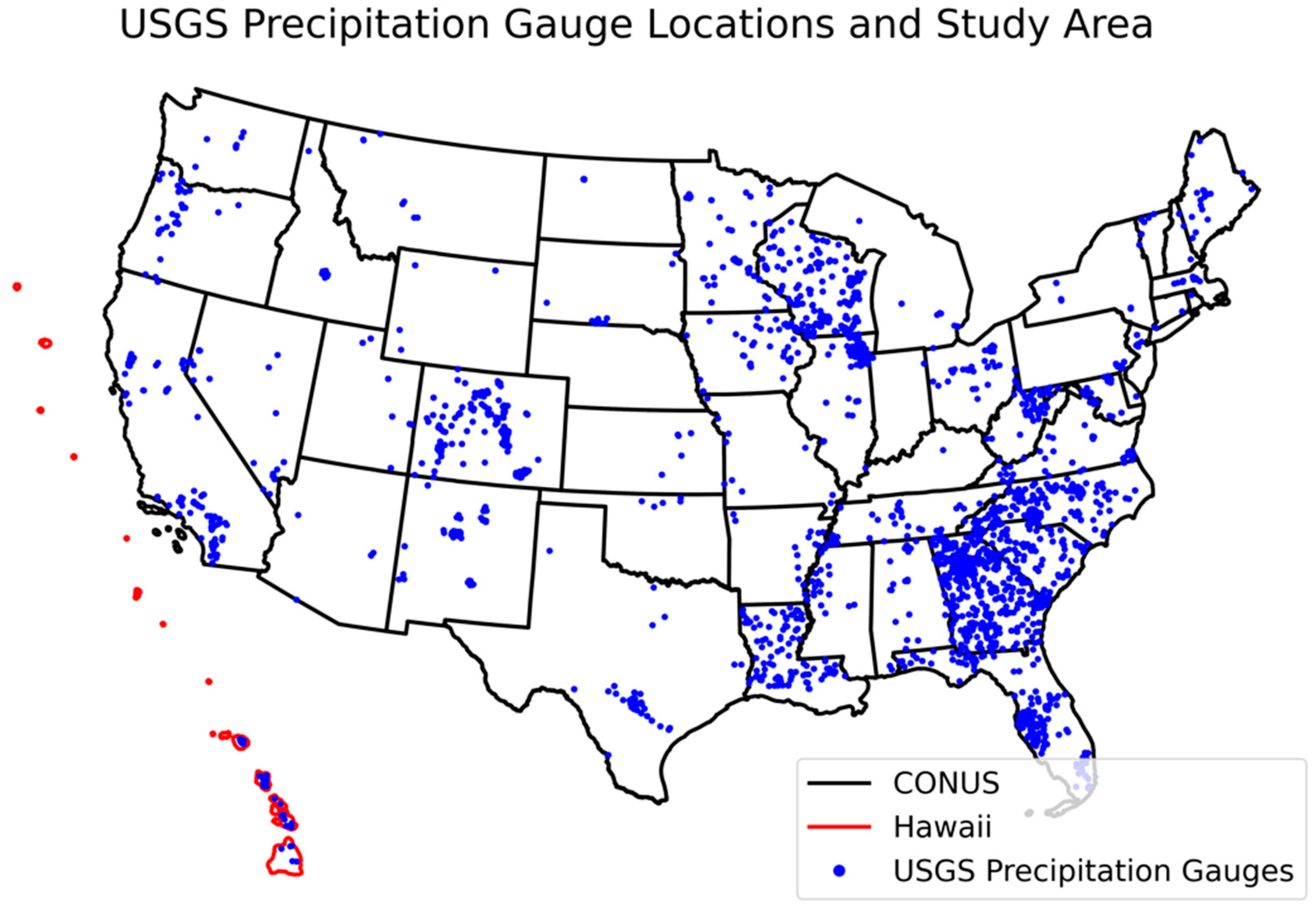
2.1. Study Area

We selected the contiguous United States (CONUS) and the state of Hawaii (HI) as the study region (Figure 1). The CONUS spans a vast area across multiple climate zones, from the arid deserts of the Southwest to the humid climates of the Southeast. This diverse region presents varying topographic features, land cover types, and precipitation regimes, providing a robust framework for evaluating satellite-based precipitation products under different environmental conditions. Hawaii, an archipelagic state located in the central Pacific Ocean, consists of several islands with complex topographies and unique climatic characteristics. The Hawaiian Islands experience a range of precipitation patterns influenced by factors such as trade winds, orographic effects, and ocean currents, offering a distinct setting for assessing the performance of satellite-based precipitation products in a tropical environment. Within and across the CONUS and Hawaii, the United States Geological Survey (USGS) maintains a dense network of precipitation. These stations provide high-quality ground-based measurements that serve as a robust reference dataset for validating SPDs. These gauges are distributed across various climatic regions, topographies, and land cover types.

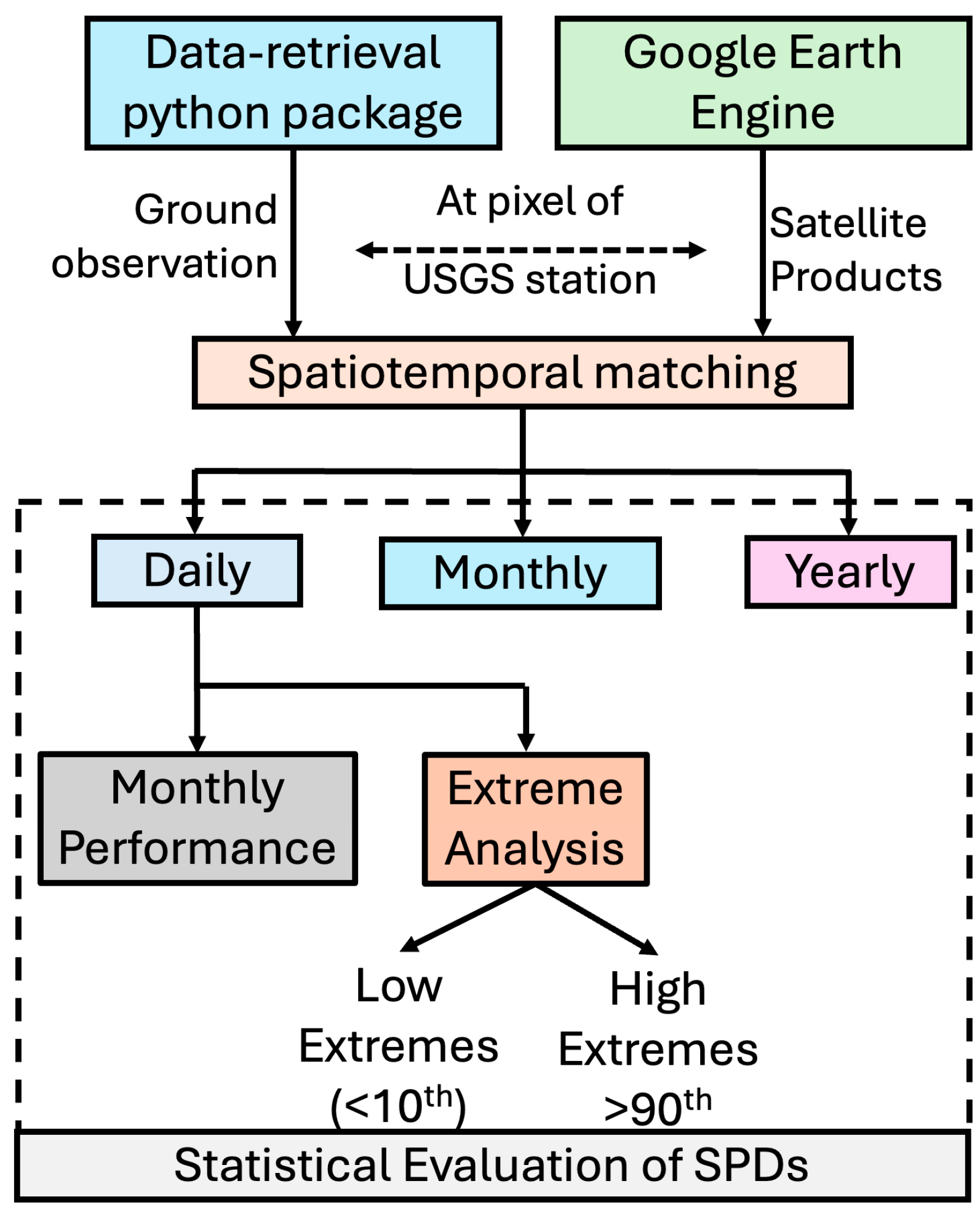
2.2. Data Collection

2.2.1. Ground-Based Precipitation Data

Ground-based precipitation data were obtained from the extensive network of precipitation gauges maintained by the USGS. Data acquisition was facilitated through the ‘dataretrieval’ Python library (version 1.0.10) [35], which interfaces with the National Water Information System (NWIS). This process involved identifying and retrieving metadata for stations recording daily precipitation values within the study area, utilizing a custom-made function in python. The metadata included station names, site numbers, and the range of available data. Initially, around 3400 stations were identified. We developed a function that, upon executing, allows users to retrieve precipitation data for each station, spanning the full period of record. However, after filtering out stations with no available data, 1237 stations were successfully retrieved and included in our analysis. These USGS gauge stations operate independently of the satellite-based precipitation-estimation systems, ensuring an unbiased reference dataset for validation of the satellite products. Rigorous quality control measures implemented by the USGS ensure the reliability and accuracy of the ground-based precipitation data.

2.2.2. Satellite-Based Precipitation Data

Satellite-based precipitation estimates were acquired using the Google Earth Engine (GEE) platform, which provides access to a vast repository of environmental datasets through the ‘ee’ Python library (version 0.1.416) [36]. This approach facilitated the extraction of multiple SPDs, each characterized by distinct spatial and temporal resolutions. We developed a custom Python class for the data collection process designed to automate the extraction of SPDs for specific areas of interest over designated time periods. This study focused on four primary SPDs (refer to Table 1 for a summary), each offering unique coverage and resolution characteristics:

• CHIRPS (UCSB-CHG/CHIRPS/DAILY): The Climate Hazards Group InfraRed Precipitation with Station data (CHIRPS) dataset is a quasi-global rainfall dataset [37] that combines satellite imagery with in-situ station data to create gridded rainfall time series for trend analysis and seasonal drought monitoring. It has a spatial resolution of approximately 5.5 km and a daily temporal resolution, covering the period from 1981 to the present;
• TERRA (IDAHO_EPSCOR/TERRACLIMATE): The TerraClimate collection offers monthly aggregated precipitation data with a spatial resolution of about 4.6 km, spanning from 1958 to the present [38]. This dataset is widely used for climatological research and environmental modeling;
• PERSIANN (NOAA/PERSIANN-CDR): The Precipitation Estimation from Remotely Sensed Information using Artificial Neural Networks-Climate Data Record (PERSIANN-CDR) provides global precipitation data derived from satellite observations [39]. It offers daily updates and has a coarser spatial resolution of 27 km, available from 1983 to the present;
• MERRA (NASA/GSFC/MERRA/slv/2): The Modern-Era Retrospective analysis for Research and Applications, Version 2 (MERRA-2) integrates satellite data with ground-based observations to provide high-quality atmospheric data [40]. The dataset features an hourly temporal resolution and a spatial resolution of 69 km, covering the period from 1980 to the present.

Table 1. Summary of Satellite Precipitation Products Used in this Study.

Satellite Product	Source ID	Temporal Resolution	Spatial Resolution	Period Covered
CHIRPS	UCSB-CHG/CHIRPS/DAILY	Daily	5.5 km	1981–2023
TERRA	IDAHO_EPSCOR/TERRACLIMATE	Monthly	4.6 km	1958–2023
PERSIANN	NOAA/PERSIANN-CDR	Daily	27 km	1983–2023
MERRA-2	NASA/GSFC/MERRA/slv/2	Hourly	69 km	1980–2023

Table 1. Summary of Satellite Precipitation Products Used in this Study.

Satellite Product	Source ID	Temporal Resolution	Spatial Resolution	Period Covered
CHIRPS	UCSB-CHG/CHIRPS/DAILY	Daily	5.5 km	1981–2023
TERRA	IDAHO_EPSCOR/TERRACLIMATE	Monthly	4.6 km	1958–2023
PERSIANN	NOAA/PERSIANN-CDR	Daily	27 km	1983–2023
MERRA-2	NASA/GSFC/MERRA/slv/2	Hourly	69 km	1980–2023

2.3. Temporal Scale Analysis

The spatial-temporal matching between satellite data and ground observations was performed as follows:

• Spatial matching: For each USGS gauge station, we extracted satellite data from the pixel containing the station’s coordinates;
• Temporal matching: We aligned the satellite data with the ground observations based on their respective timestamps, ensuring a one-to-one correspondence for each time step (daily, monthly, or yearly);
• Data gaps: Any missing data in either the satellite or ground observations were excluded from the analysis to ensure consistent comparisons;
• Time zone considerations: All timestamps were converted to a standard time zone (UTC) to avoid discrepancies due to different local time zones across the study area.

After that, we employed several performance metrics, such as the coefficient of determination (R²), root mean squared error (RMSE), mean squared error (MSE), and mean absolute error (MAE) using sklearn python library (version 1.5.1) [41], to assess the efficacy of the SPDs against ground-based precipitation data. These metrics were calculated to understand the predictive accuracy and error rates of the satellite data relative to the gauge data. The analysis was structured to evaluate the datasets on daily, monthly, and yearly time scales.

2.3.1. Daily Analysis

Satellite data from CHIRPS, PERSIANN, and MERRA were used to create a daily time series of precipitation (TERRA was excluded due to its monthly temporal resolution). Each dataset was aligned with the daily aggregated USGS gauge data based on the date ranges specified. For MERRA, which is available in hourly resolution, we summed the hourly precipitation data to convert them into daily totals.

2.3.2. Monthly Analysis

For the monthly scale, daily precipitation data from PERSIANN, CHIRPS, and MERRA were summed to create a monthly time series. TERRA, already at a monthly scale, was also included. This was compared with the monthly aggregated USGS data.

2.3.3. Yearly Analysis

The yearly analysis aggregated the daily or monthly data into annual totals for those satellites capable of providing daily or monthly outputs, respectively, and compared these against the annual aggregates of USGS data.

The calculation of these indices was automated using a Python script, which processed the datasets efficiently and stored the results in designated folders for each index and temporal resolution. This approach not only facilitated a detailed comparison across different timescales but also streamlined the handling and analysis of large datasets. This methodology provides a robust framework for evaluating the spatial accuracy and temporal reliability of satellite precipitation estimates, which is essential for enhancing their application in various hydrological and climatological applications. For each ground location, the SPD with the highest performance score (e.g., highest R², lowest RMSE) was identified as the best-performing SPD on the daily, monthly, and yearly temporal scales. The best-performing SPDs were then mapped spatially by labeling each location according to the optimal SPD. Separate maps were generated for each temporal scale, enabling the identification of regional patterns and the selection of the most suitable SPD for specific locations.

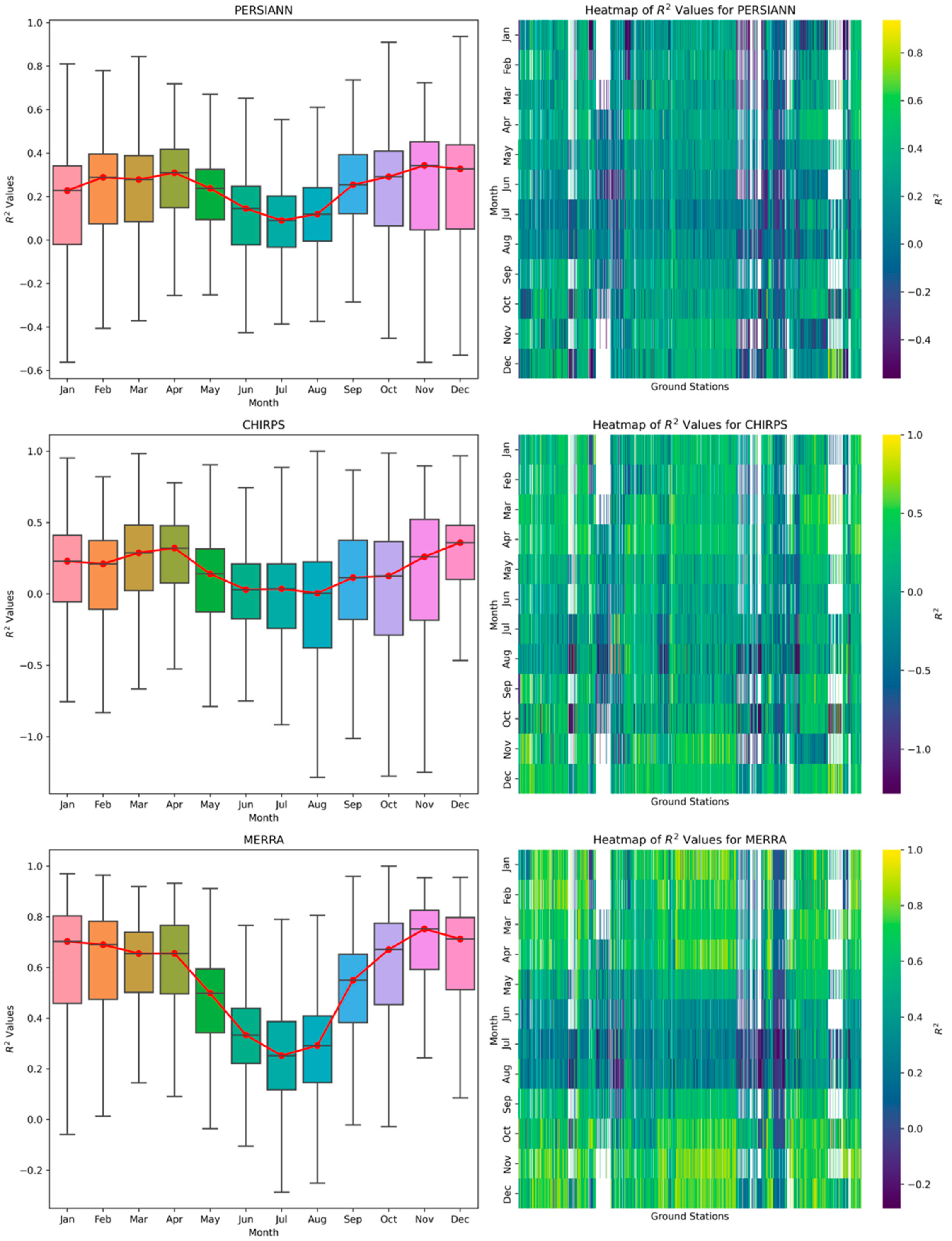
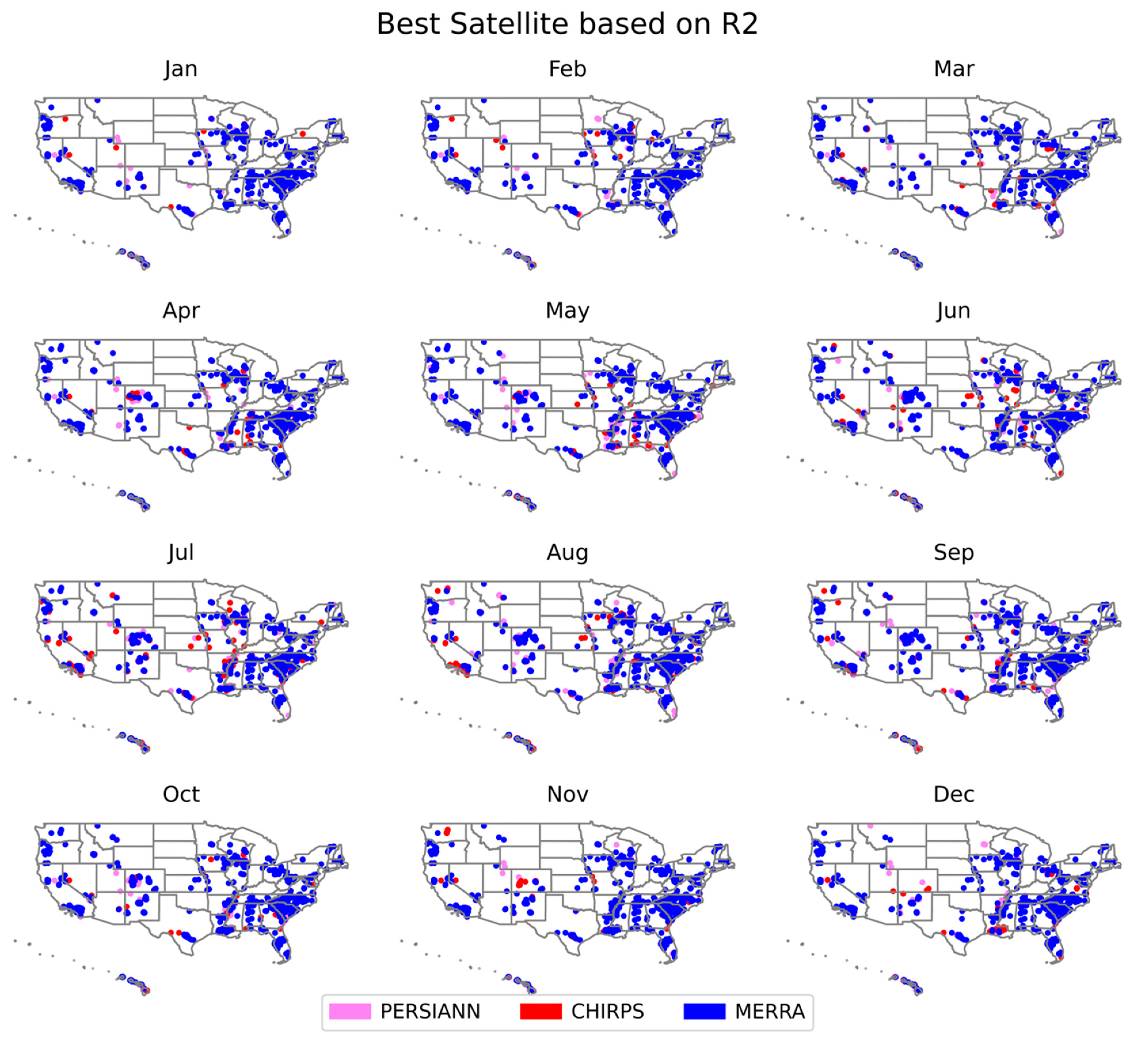
2.4. Monthly Performance Analysis

An examination of the monthly performance of SPDs at the daily scale was conducted to evaluate seasonal variations and monthly accuracy trends. Prior to the calculation of performance indices, the data were preprocessed to handle outliers using the interquartile range (IQR) method. The IQR, defined as the difference between the 75th and 25th percentiles, was used to identify and filter extreme values falling outside the range of (Q1 − 1.5 * IQR, Q3 + 1.5 * IQR), where Q1 and Q3 represent the first and third quartiles, respectively. This outlier-removal step ensured the robustness of the subsequent analysis by mitigating the impact of anomalous measurements. The performance indices—R², MSE, RMSE, and MAE—were then calculated for each month. This setup facilitated the evaluation of how well each SPD predicted the observed precipitation across different months, highlighting any discrepancies or biases that might exist in specific periods of the year. The results were structured to provide a clear monthly breakdown of each performance metric for each site, allowing for an in-depth analysis of temporal trends. This approach not only provided a snapshot of the overall accuracy but also highlighted the variability in satellite data performance throughout the year. Monthly analysis helps identify specific months where satellite data may underperform or outperform, which is crucial for improving the calibration of satellite models and enhancing their application in real-world scenarios. Moreover, understanding the monthly variability in satellite data accuracy can lead to better resource management and decision-making processes, particularly in sectors sensitive to seasonal climatic changes.

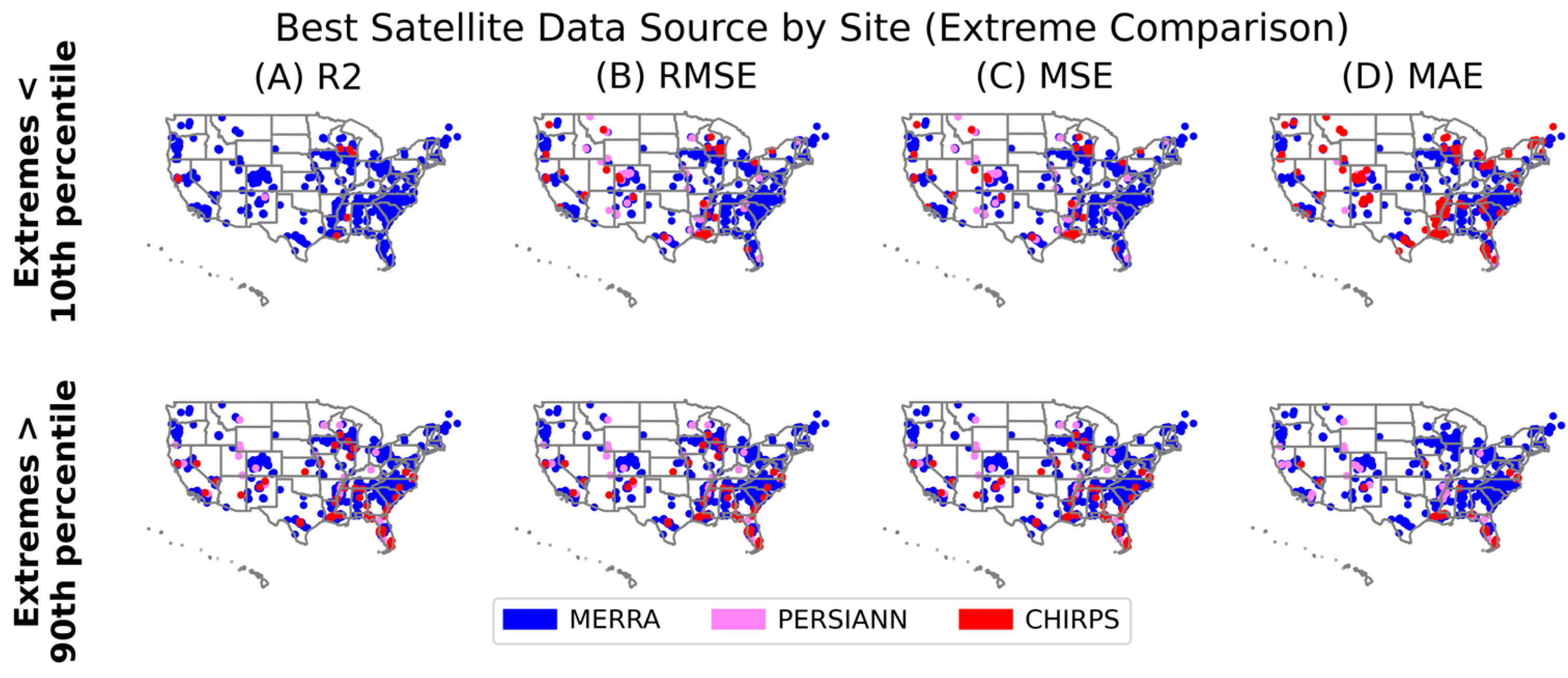
2.5. Extreme Precipitation Analysis

To assess the effectiveness of the satellite precipitation datasets (SPDs) in simulating extreme precipitation events, we conducted a comparative analysis using data below the 10th percentile and above the 90th percentile of observed precipitation. This analysis was performed at the daily timescale for the SPDs PERSIANN, CHIRPS, and MERRA. We calculated the 10th and 90th percentile thresholds for each site using ground-based USGS measurements. For data below the 10th percentile, we identified the days with precipitation values lower than this threshold. Similarly, for data above the 90th percentile, we identified the days with precipitation values higher than this threshold. The satellite precipitation data were then filtered to match these extreme events. We employed the same performance metrics (R², RMSE, MSE, and MAE) as described in Section 2.3 to evaluate the SPDs during extreme precipitation events. To visually represent the performance of each SPD in capturing extreme events, we generated spatial maps indicating the best-performing dataset at each site based on the evaluated metrics. The maps were categorized into two rows: one for events below the 10th percentile and one for events above the 90th percentile. Each row includes four panels representing R², RMSE, MSE, and MAE. The color coding used was blue for MERRA, red for CHIRPS, and violet for PERSIANN. The overall methodology adopted in this study is shown in Figure 2.

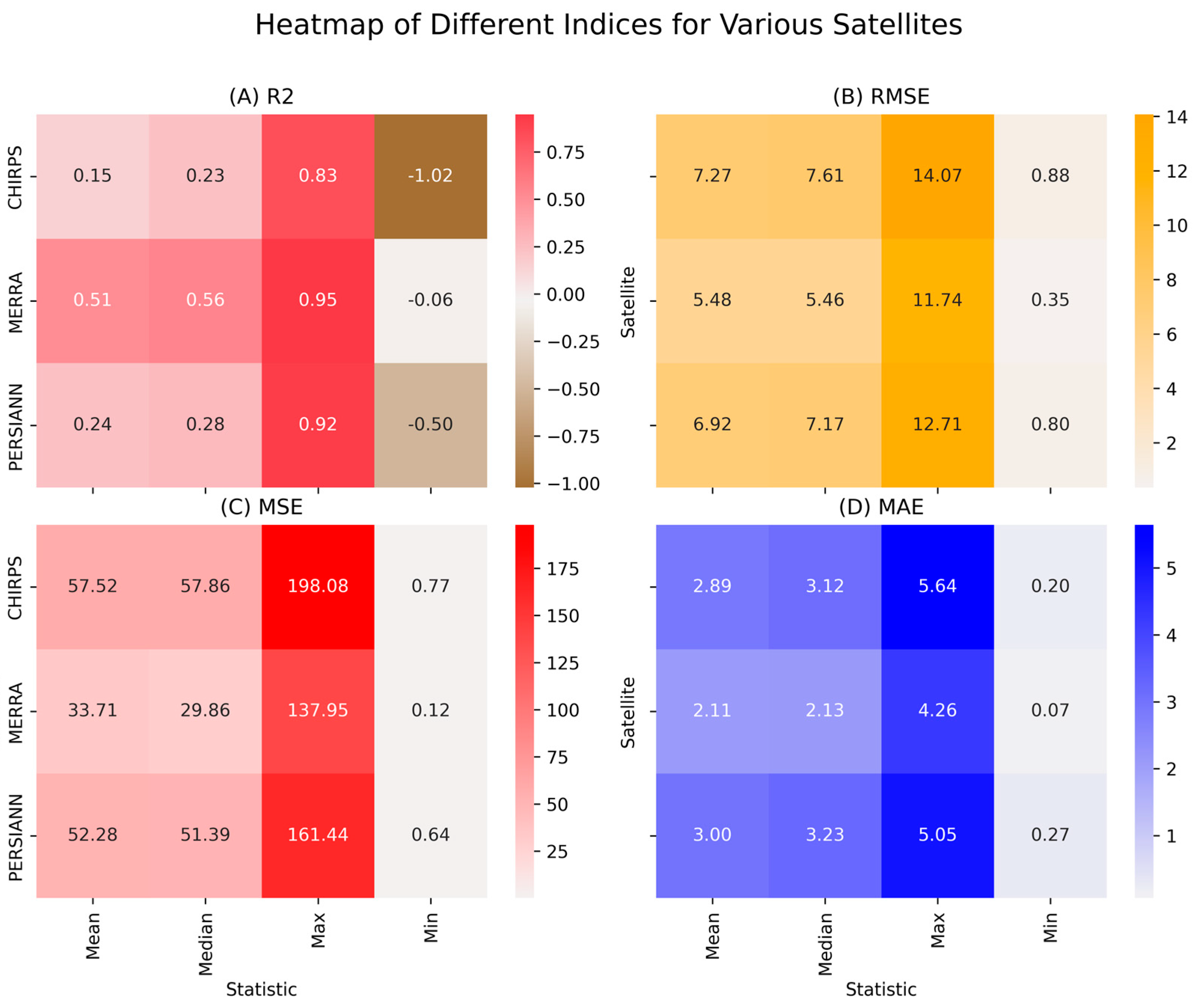
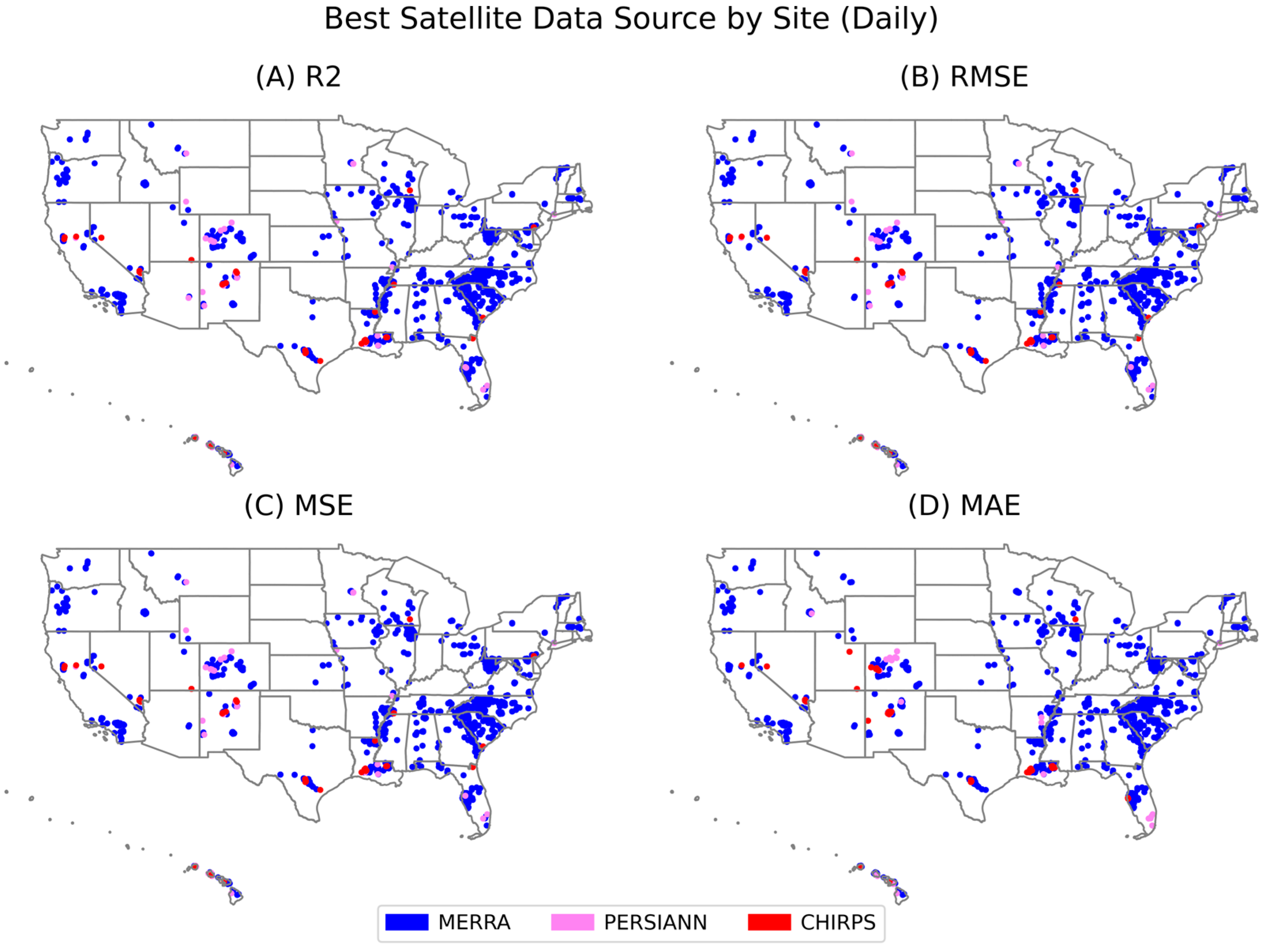
3. Results

3.1. Temporal Scale Analysis

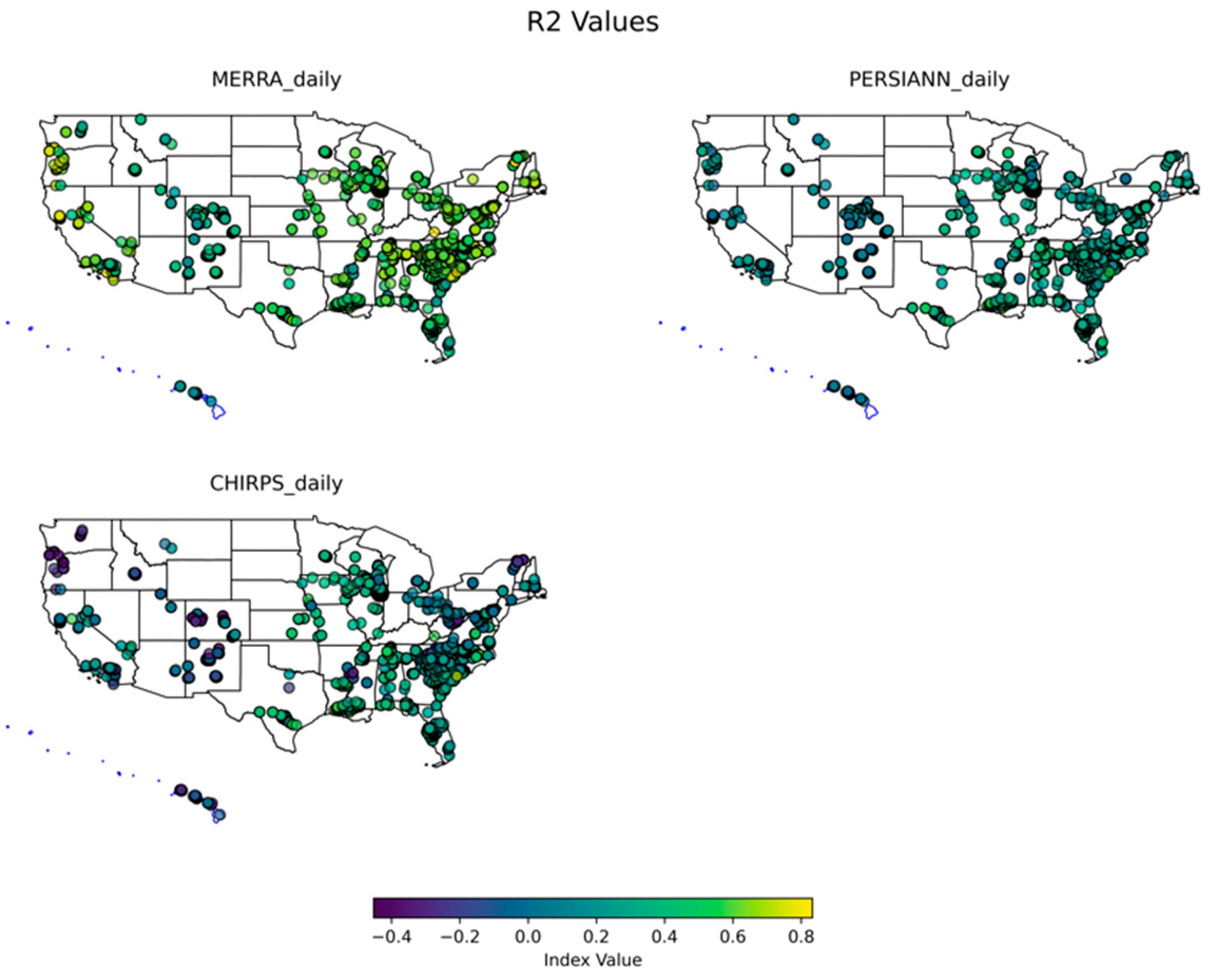
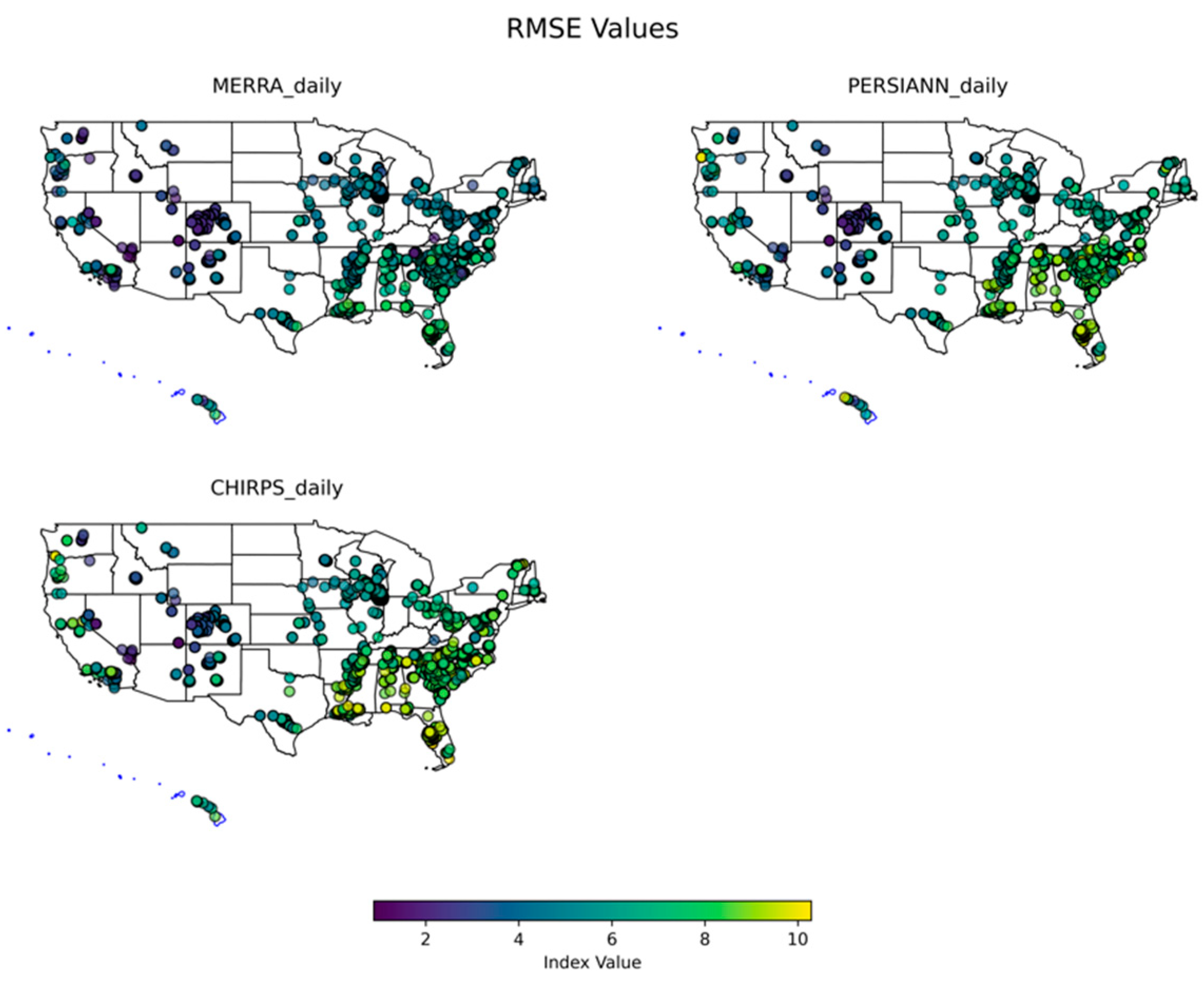
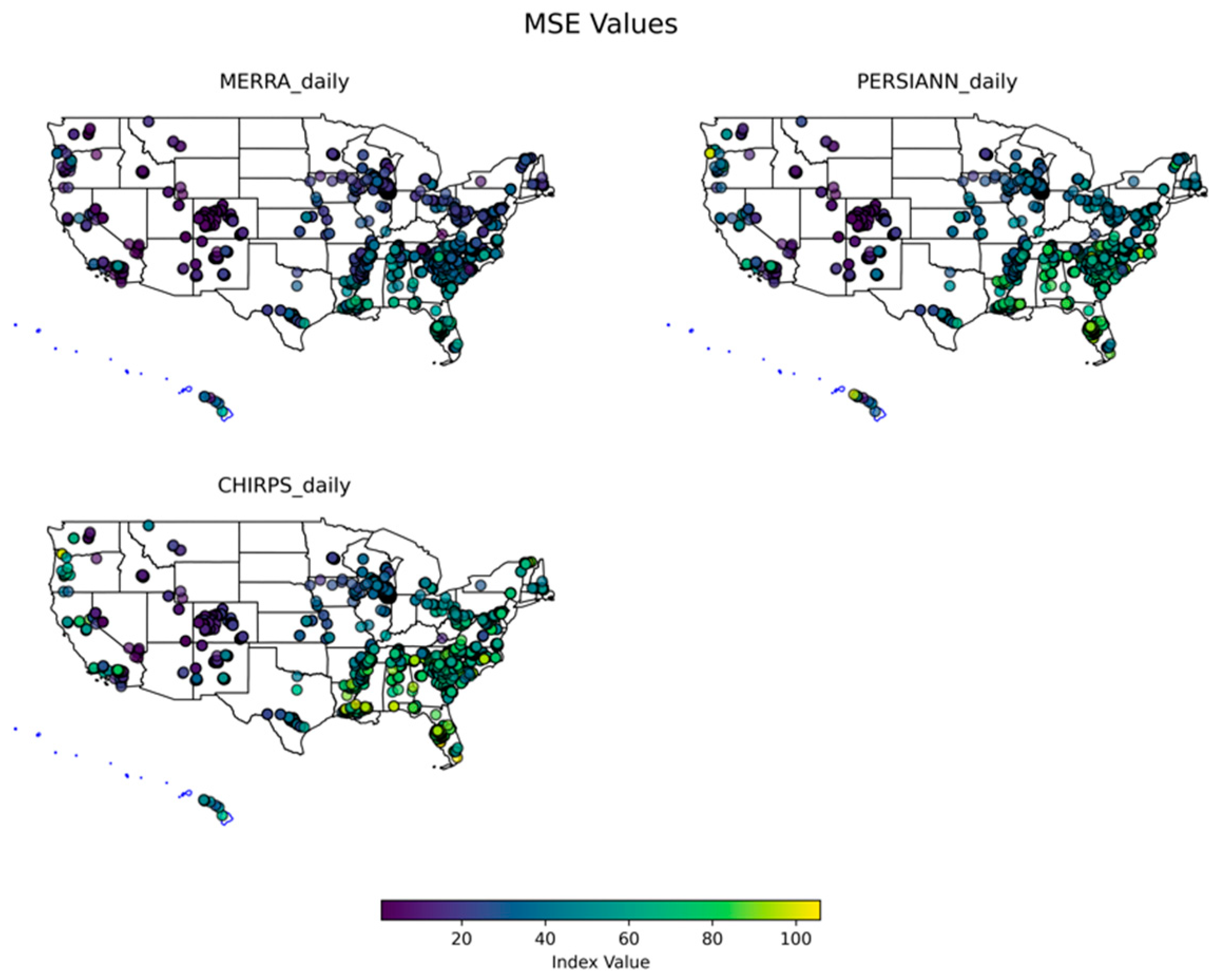
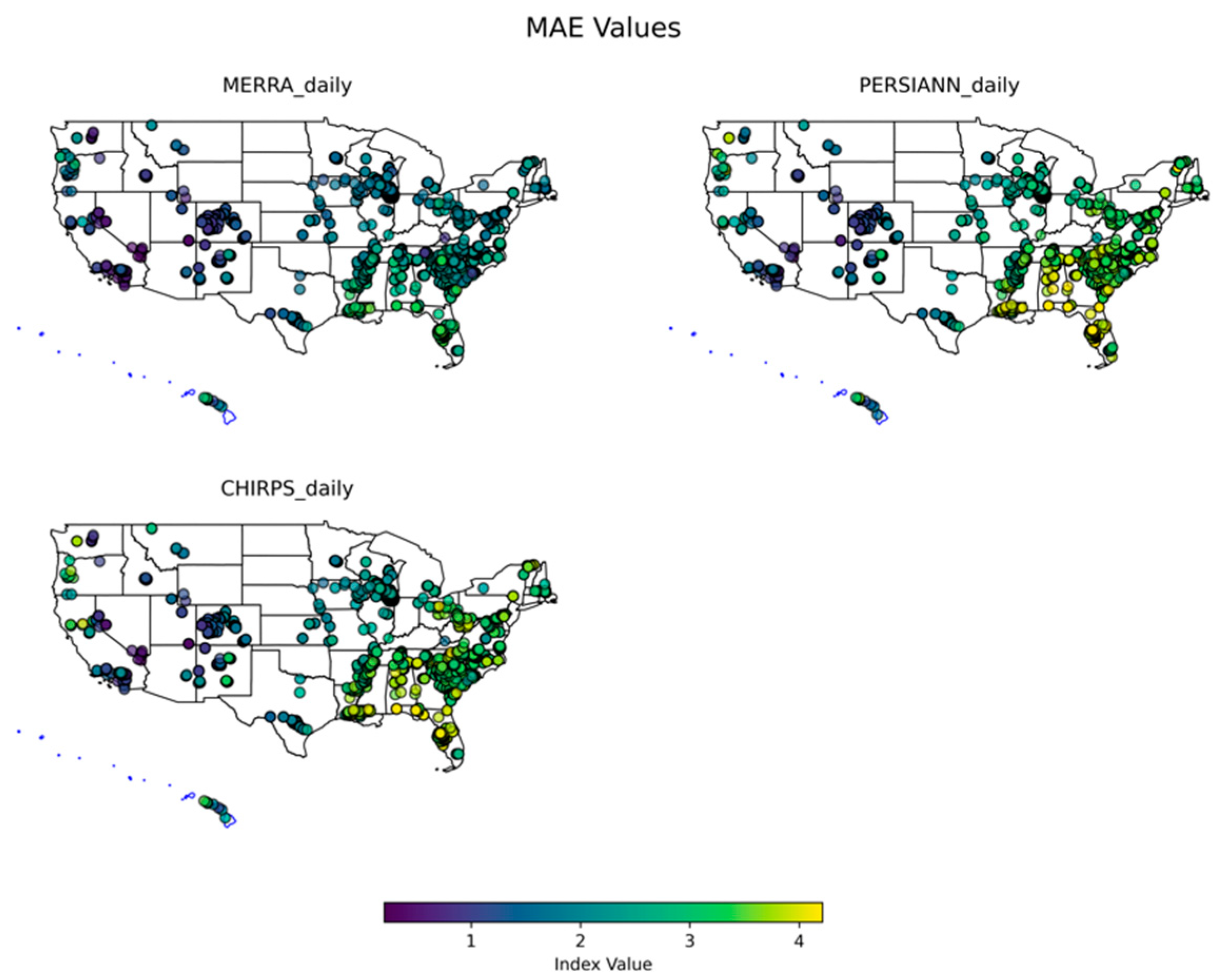
3.1.1. Daily

We found that CHIRPS exhibited a moderate correlation (mean R² = 0.146, and median R² = 0.225) with the ground observations. However, the R² values ranged from −1.022 to 0.833, suggesting significant inter-station variability in its performance across different regions or conditions. In terms of error quantification, CHIRPS demonstrated a relatively high RMSE (7.267 mm), MAE (2.888 mm), and MSE (57.519 mm). PERSIANN demonstrated a higher mean R² of 0.239 and a median R² of 0.277, reflecting a better overall correlation with ground-based observations than CHIRPS. Its R² values ranged from -0.501 to 0.923, indicating a more consistent performance than CHIRPS. PERSIANN’s RMSE (6.919 mm) and MSE (52.277 mm) were lower than those of CHIRPS, suggesting improved accuracy. Additionally, its MAE (2.997 mm) was slightly higher than that of CHIRPS. MERRA outperformed the two above-mentioned SPDs, exhibiting the highest mean R² of 0.506 and a median R² of 0.555. Its R² values ranged from −0.063 to 0.948, demonstrating a consistently high performance. MERRA had the lowest RMSE (5.480 mm) and MSE (33.706 mm) values among the three SPDs. Furthermore, its MAE (2.113 mm) was the lowest, suggesting the smallest average deviation from ground-based observations. The statistical summary of the satellite precipitation data is presented in a heatmap in Figure 3 and the spatial representation of these indices —R², RMSE, MSE, and MAE— (Figure A1, Figure A2, Figure A3 and Figure A4 respectively) provides a visual representation of the performance of each SPD spatially.

The spatial distributions of the indices (Figure A1, Figure A2, Figure A3 and Figure A4) reveal that the satellite-based precipitation estimates perform comparatively better in the southeastern US and western California, particularly MERRA. Higher values of R² and lower values of the RMSE, MSE, and MAE in these regions indicate that MERRA provides more accurate precipitation estimates compared to other regions. Figure 4 is a spatial representation of the best-performing satellite, based on the R², RMSE, MSE, and MAE values. Most stations are dominated by MERRA, indicating its superiority. However, some states, including Louisiana, Texas, New Mexico, and Colorado, exhibit some CHIRPS and PERSIANN sporadically, although a closer examination of the values reveals that the differences are relatively minor. This spatial analysis further reinforces the overall finding that MERRA outperforms the other two SPDs in capturing daily precipitation patterns across the US.

3.1.2. Monthly

Interestingly, for the monthly timescales, CHIRPS emerges as the top-performing SPD across the US. It exhibits the highest mean R² of 0.554 and the highest median R² of 0.660, indicating a strong overall correlation with the ground observations. The R² values for CHIRPS ranged from −1.342 to 0.943, suggesting reliable performance. CHIRPS also demonstrated the lowest RMSE (34.687 mm) and MSE (1407.271 mm) values among the SPDs, reflecting its high accuracy in estimating monthly precipitation totals. Furthermore, its MAE (25.092 mm) is the smallest, implying the smallest average deviation. MERRA, which outperformed the other SPDs for daily precipitation, ranks second for monthly data. Its mean R² of 0.1 and median R² of 0.603 are lower than those of CHIRPS but still indicate a good correlation with the ground observations. MERRA’s RMSE (37.174 mm) and MSE (1633.471 mm) are slightly higher than those of CHIRPS, but its MAE (26.602 mm) is lower than those of PERSIANN and TERRA. TERRA follows closely behind MERRA, with a mean R² of 0.402 and median R² of 0.481. Its RMSE (42.028 mm) and MSE (2055.528 mm) are higher than those of CHIRPS and MERRA, but its MAE (30.354 mm) is better than that of PERSIANN. PERSIANN exhibits the lowest performance for monthly precipitation estimates, with a mean R² of 0.266 and median R² of 0.424. It also has the highest RMSE (44.444 mm), MSE (2254.745 mm), and MAE (33.172 mm) among the SPDs, indicating relatively higher errors and deviations from the ground measurements. The statistical summary is shown in Figure 5. Also, the spatial distribution of the indices R², RMSE, MSE, and MAE are available in Figure A5, Figure A6, Figure A7 and Figure A8, respectively.

Figure 6 shows the spatial distribution of the best-performing SPD at each ground station location for monthly precipitation, based on the R², RMSE, MSE, and MAE values. Notably, most stations are dominated by CHIRPS, indicating its superior statistical values. MERRA is the second most prevalent, suggesting its strong performance relative to the other SPDs.

Upon closer examination of the values, the differences between CHIRPS and MERRA were found to be relatively minor, indicating comparable accuracy for many stations. We found that PERSIANN is rarely the best-performing SPD, appearing at only about 10 stations. Notably, TERRA exhibited the best estimation in Colorado, indicating its strength in capturing monthly precipitation patterns. Furthermore, TERRA’s accuracy is nearly on par with CHIRPS and MERRA for monthly timescales across multiple locations, underscoring its reliability for monthly precipitation estimates. This spatial analysis reinforces the overall finding that CHIRPS outperforms the other SPDs in estimating monthly precipitation totals across the US, with MERRA and TERRA also exhibiting strong performance in various regions. However, the relatively minor differences between CHIRPS and MERRA (TERRA in Colorado) highlight the importance of carefully evaluating the specific requirements and characteristics of the study area when selecting the appropriate SPD for monthly timescales.

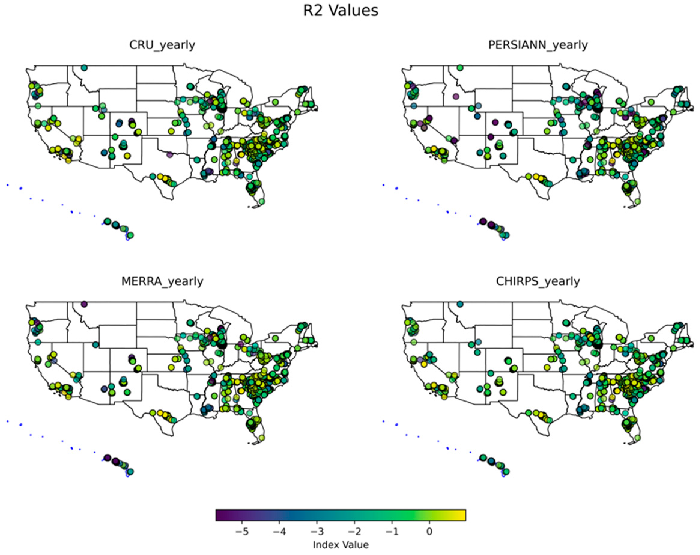
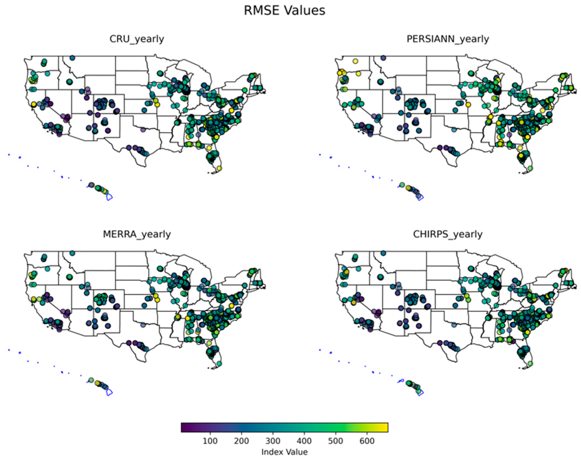
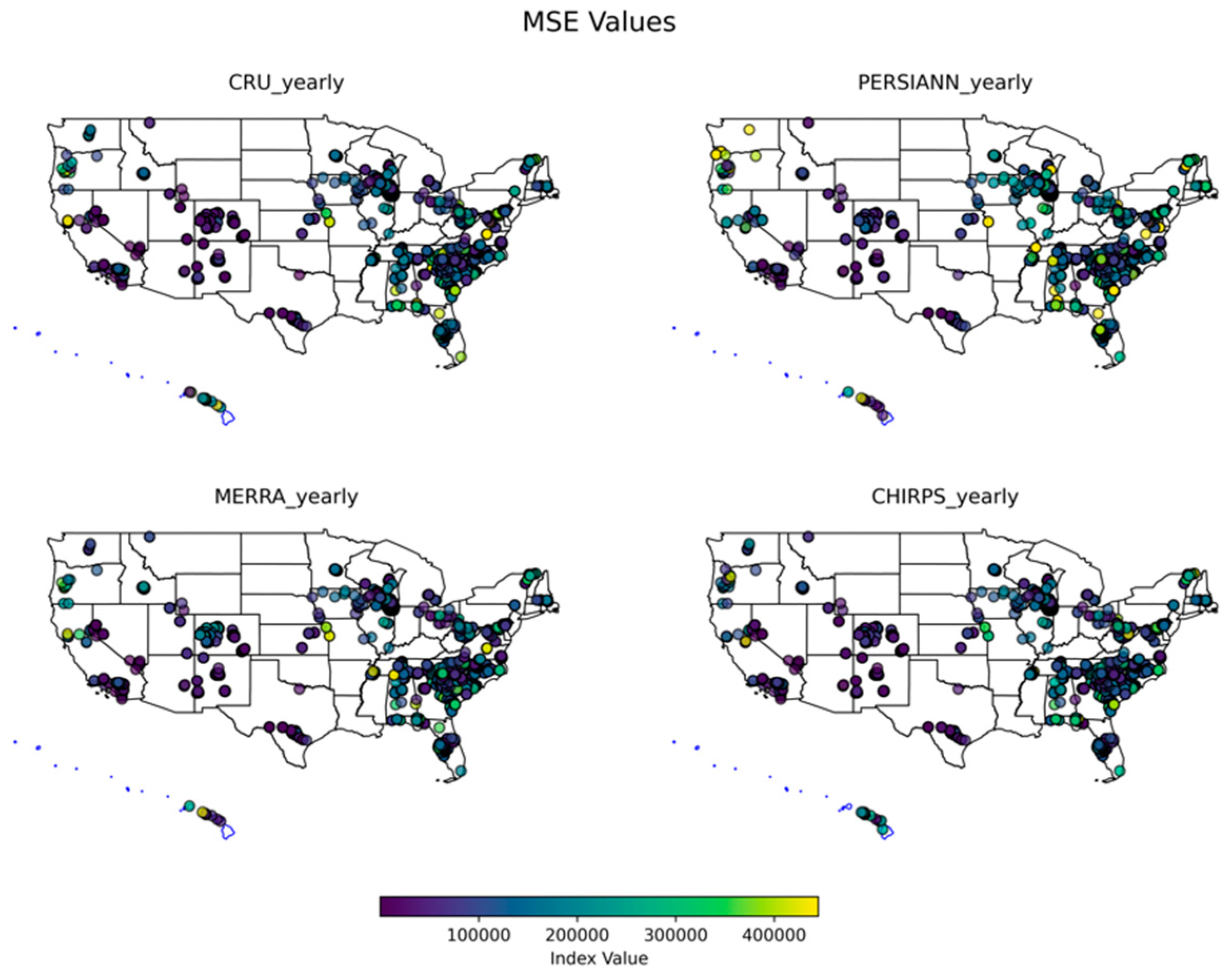
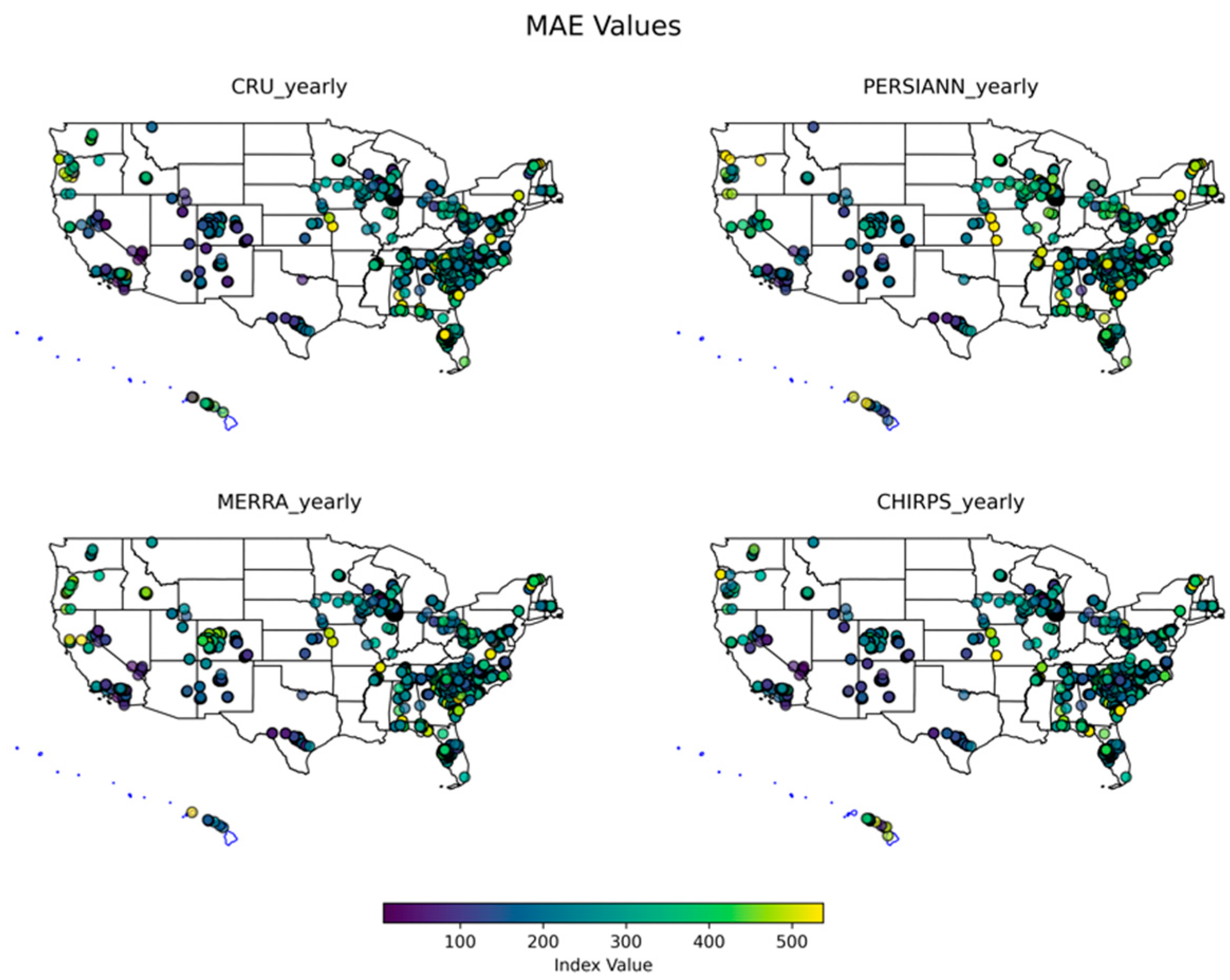
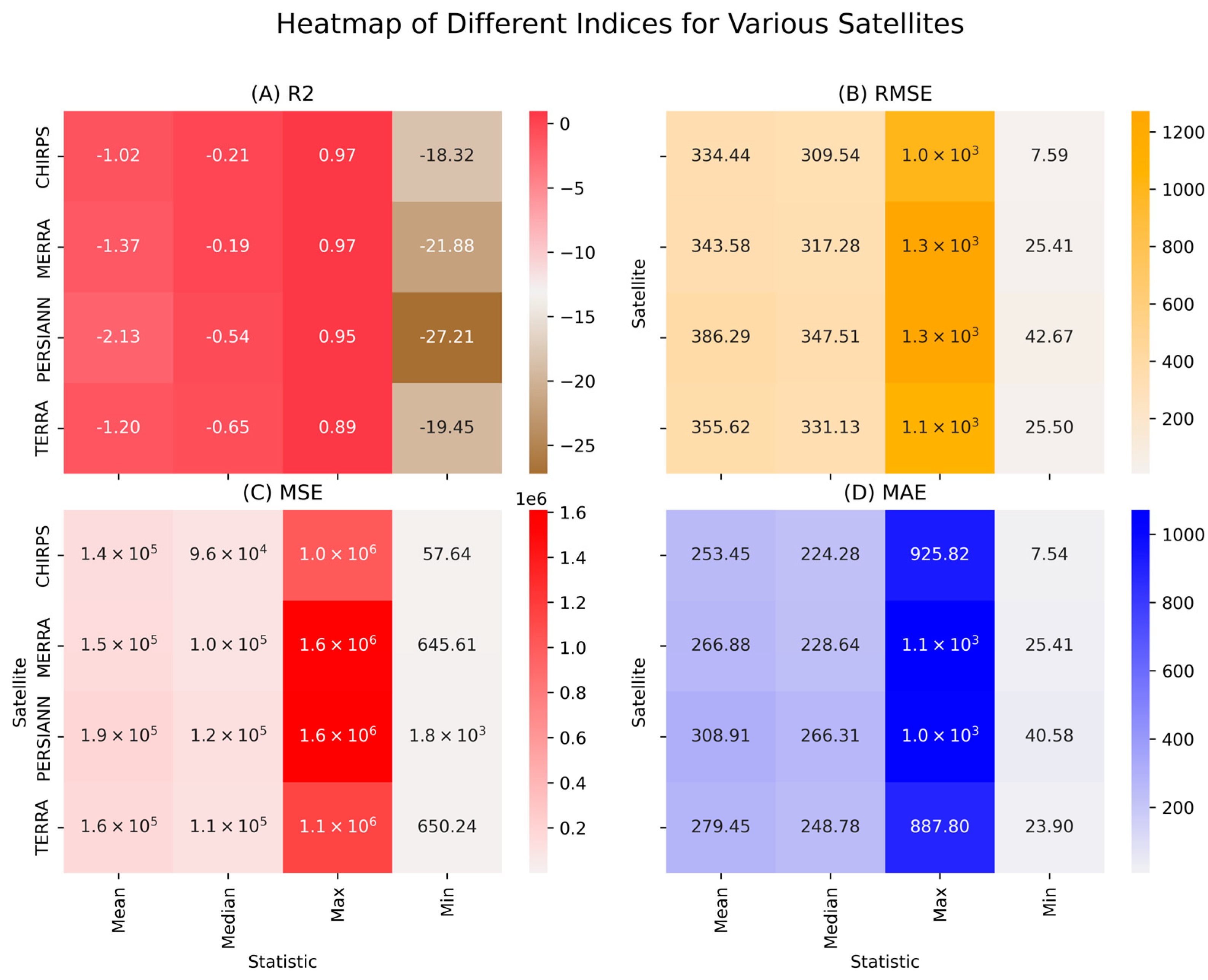
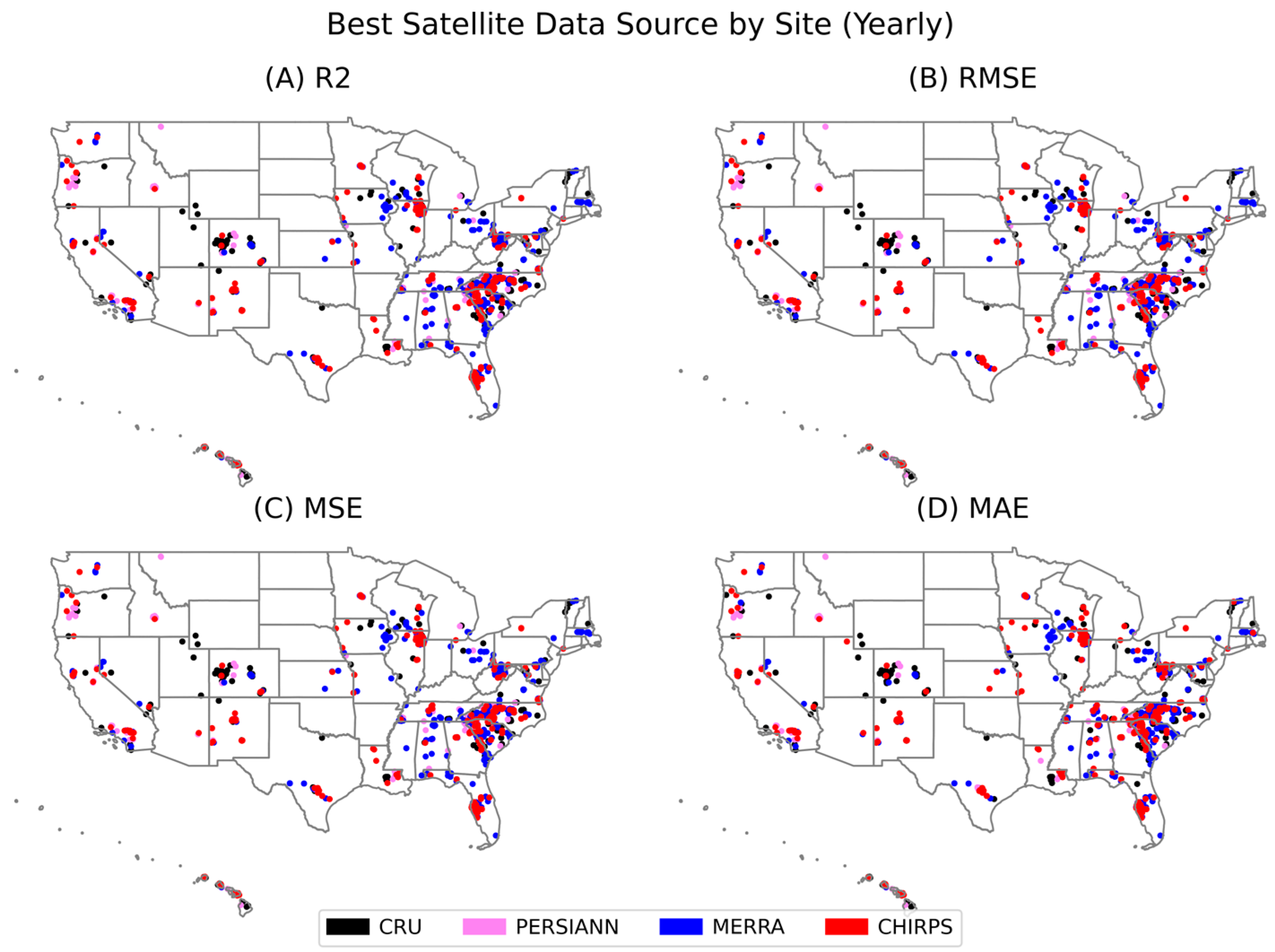
3.1.3. Yearly

Figure A13 presents the statistical performance metrics for the annual precipitation totals from SPDs across the US. It is evident that the annual sum of precipitation is predicted relatively poorly by all SPDs when compared to the monthly and daily timescales. On an annual scale, none of the datasets exhibit satisfactory R² values, with means ranging from −2.131 (PERSIANN) to −1.023 (CHIRPS). The negative values indicate a lack of correlation with the ground observations. The median R² values, although less negative, are still low, with the highest being −0.194 for MERRA. The RMSE and MAE values are relatively high for all datasets, suggesting significant errors in estimating annual precipitation totals. CHIRPS has the lowest RMSE (334.438 mm) and MAE (253.454 mm), closely followed by MERRA. However, these values are still substantially higher than those observed for the monthly and daily timescales. Similarly, the MSE values are alarmingly high, with PERSIANN exhibiting the highest mean MSE (185191.89 mm), indicating substantial deviations from the ground-based observations. The poor performance of all SPDs in estimating annual precipitation is further highlighted by the wide ranges of statistical values. For instance, the R² values range from −27.210 to 0.950 for PERSIANN, and the RMSE values range from 25.409 mm to 1263.697 mm for MERRA, indicating significant variability and uncertainty. These results clearly demonstrate that the SPDs struggle to accurately predict the annual precipitation across the US. The lack of correlation and high error values suggest that caution should be exercised when using these datasets for applications that require precise annual precipitation estimates.

Looking at the spatial representation of the best-performing SPD for annual precipitation totals (Figure A13), the pattern is largely like that observed for the monthly timescales. Most stations are dominated by CHIRPS, followed by MERRA. PERSIANN and TERRA rarely emerge as the top choice across the country. The spatial distributions of the indices R², RMSE, MSE, and MAE are available in Figure A9, Figure A10, Figure A11 and Figure A12. We can see that the highest R² and lowest RMSE, MSE, and MAE values are demonstrated by CHIRPS. However, due to the overall very low statistical values observed in the table, the accuracy of these annual precipitation estimates from the SPDs should be interpreted with caution. The observed discrepancies in the annual-scale metrics may be due to the aggregation effect [42], reduced sample size [43], and potential temporal mismatches [44], which can amplify errors and reduce robustness at longer timescales. Despite exhibiting the best performance relative to the other datasets, the negative mean R² values and high RMSE, MSE, and MAE values for CHIRPS and MERRA underscore the significant challenges in attaining accurate estimations.

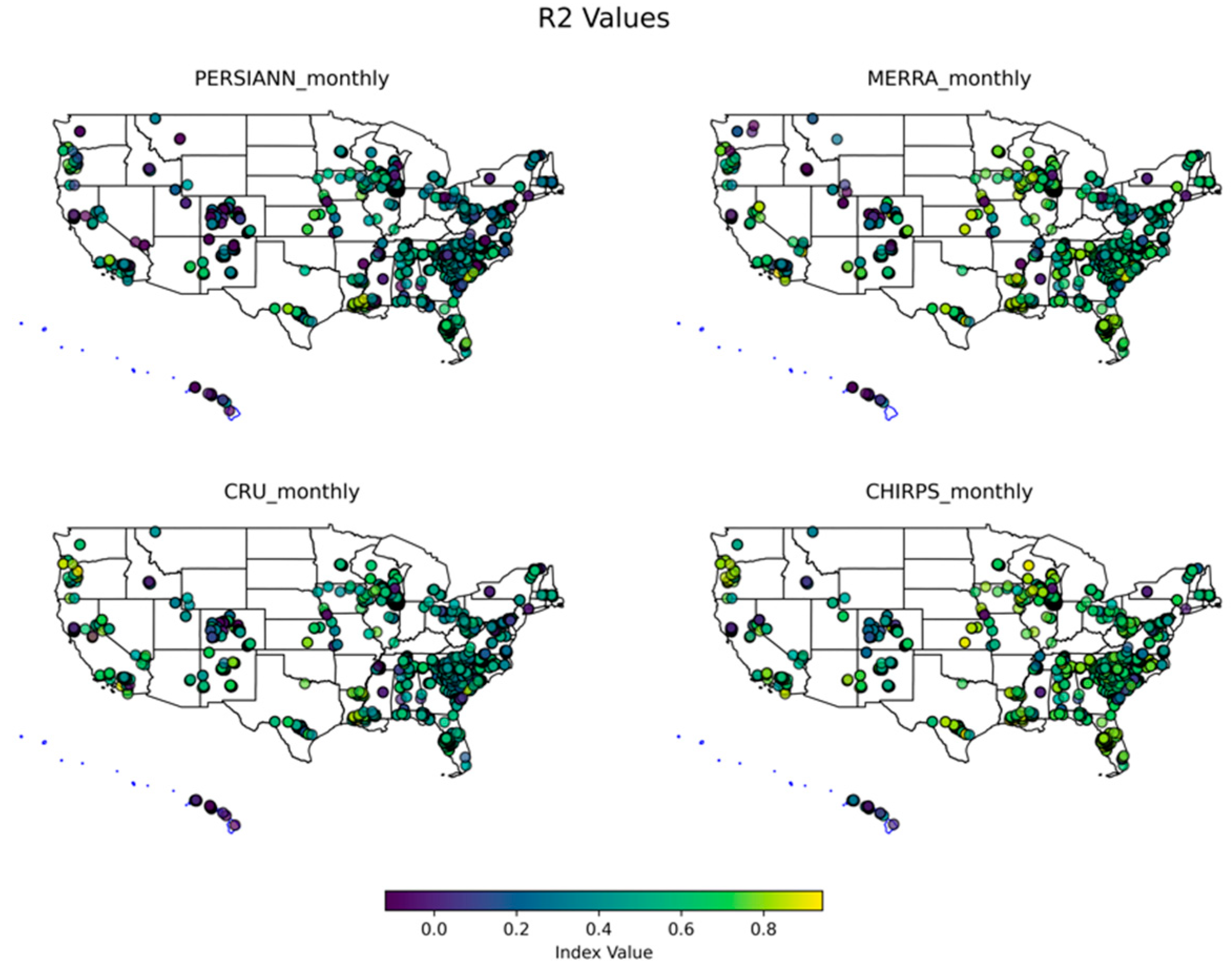
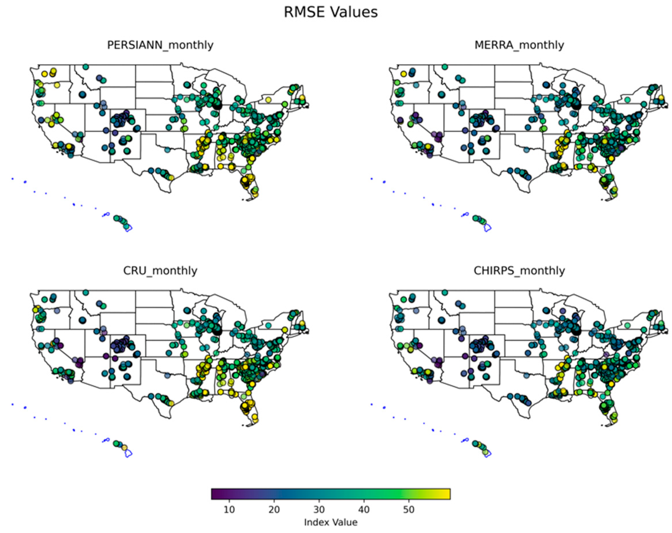
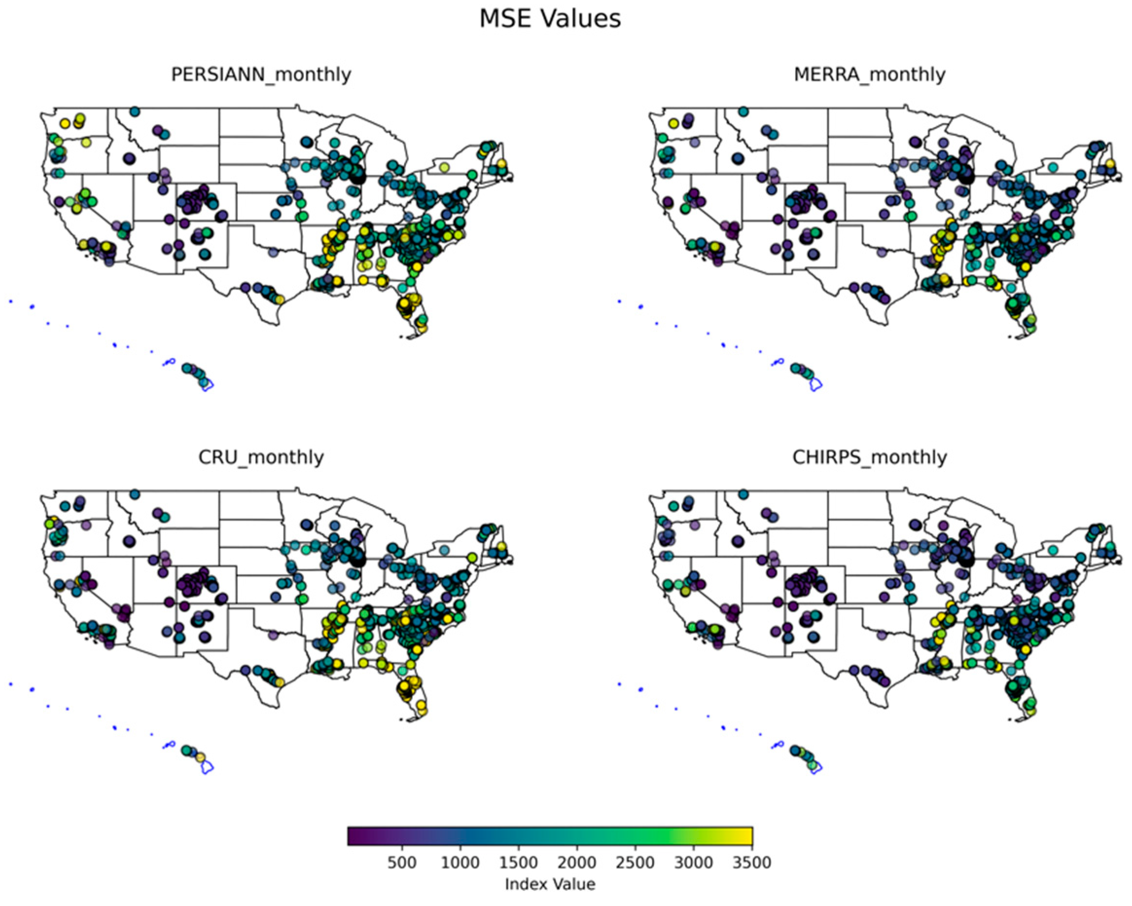
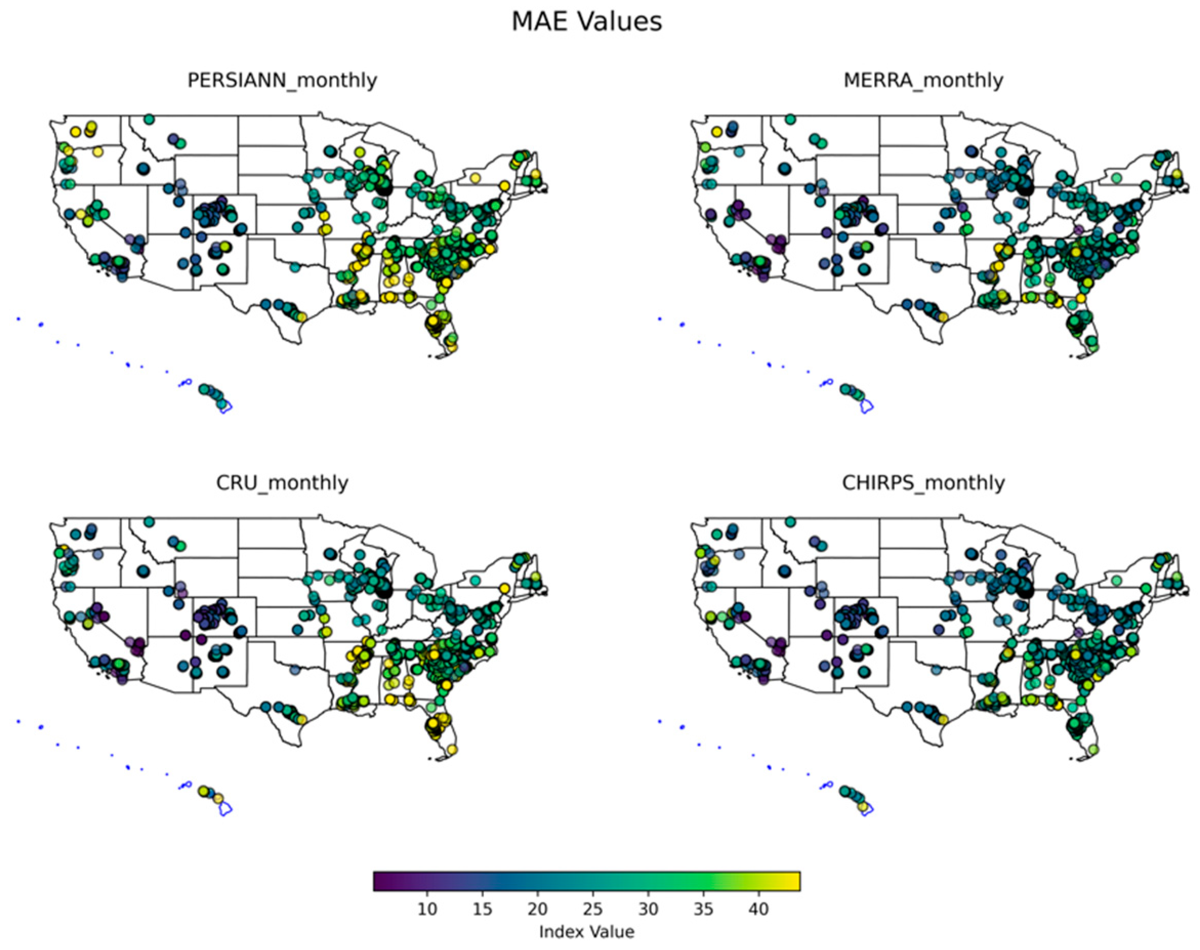
3.2. Monthly Performance Analysis

Figure 7 presents a comprehensive analysis of the monthly performance of three SPDs—PERSIANN, CHIRPS, and MERRA—compared to ground-based USGS measurements. The box plots reveal a consistent pattern across all three SPDs, with their performances fluctuating throughout the year. The median R² values exhibit a distinct trend, rising from January to April, reaching a peak in April. Subsequently, the median values decline, hitting a minimum in July, before recovering and attaining another maximum in November or December. This seasonal variation in satellite performance is particularly evident in the dip observed during May, June, July, August, and September, with July consistently showing the worst performance across all SPDs. While the overall pattern of performance variability remains similar among the SPDs, there are notable differences in the magnitudes of the R² values. MERRA demonstrates the highest median R² values, ranging from 0.25 to 0.72, indicating superior performance compared to PERSIANN (from 0.15 to 0.38) and CHIRPS (from 0.1 to 0.4). The box plots also reveal that the distribution of R² values above the median is more compact, suggesting less variability in the upper range of performance for all datasets.

Heatmaps complement the findings from the box plots, providing a spatial perspective on the monthly performance of each SPD across all stations. MERRA exhibits a greater prevalence of higher R² values, compared to PERSIANN and CHIRPS, confirming its overall better performance. When comparing CHIRPS and PERSIANN, CHIRPS displays relatively higher R² values, indicating slightly better performance. The heatmaps also highlight the monthly variance in performance, with higher R² values being more prominent in months other than those from May to August, which are dominated by lower R² values. This observation aligns with the monthly variability seen in the box plots. A closer examination of MERRA’s heatmap reveals patterns consistent with the box plot analysis, reinforcing the robustness of the findings. It is equally important to note that blank spots in the heatmaps indicate either missing data in the merged dataset or insufficient merged data points to calculate R². These gaps do not detract from the overall analysis but rather underscore the importance of data completeness and consistency in evaluating satellite precipitation estimates.

Figure 8 provides a spatial representation of the best-performing SPD for each station based on the highest R² values. The subplots cover all months from January to December, offering a comprehensive view of the spatial variability in satellite performance throughout the year. The predominance of MERRA reinforces the earlier findings confirming that MERRA consistently outperforms CHIRPS and PERSIANN in most locations and months.

However, the spatial plot also reveals some interesting patterns and exceptions. CHIRPS is the second most prevalent after MERRA, indicating that CHIRPS is the best-performing satellite for certain stations and months. This is particularly noticeable in June, July, and August, where a concentration of CHIRPS is observed in Kansas. Additionally, a cluster of CHIRPS is evident in Colorado during November. In April and May, southern Alabama also exhibits a cluster of CHIRPS. The presence of PERSIANN, although relatively sparse, signifies some areas where PERSIANN exhibits superior performance compared to the other two SPDs. These random occurrences of PERSIANN across the subplots demonstrate that PERSIANN can occasionally outperform MERRA and CHIRPS in specific locations.

3.3. Extreme Precipitation Analysis

Figure 9 presents a spatial representation of the best-performing satellite precipitation dataset at each ground station for extreme events, based on the four statistical parameters: R², RMSE, MSE and MAE. The analysis is divided into two categories: extremes below the 10th percentile and extremes above the 90th percentile.

We can see that MERRA is the best-performing dataset across most regions of the US for both low and high extremes. However, the results for low extremes (below the 10th percentile) indicate some spatial variability. While MERRA dominates, CHIRPS also shows good performance in certain locations, particularly in terms of the RMSE, MSE, and MAE. For high extremes (above the 90th percentile), the number of locations where CHIRPS performs better increases compared to the low extremes. Although MERRA remains the best-performing dataset overall, more regions show better results with CHIRPS, and to a lesser extent, PERSIANN. This indicates that, while MERRA is generally reliable, CHIRPS has strengths in capturing high extreme precipitation events in specific areas. These observations suggest that, while MERRA provides robust performance across different metrics and extremes, CHIRPS and PERSIANN can be valuable in specific regional contexts, especially for high extreme events. This highlights the importance of considering regional and event-specific characteristics when selecting the most suitable satellite precipitation dataset for extreme event analysis.

4. Discussion

A comprehensive analysis of SPDs at various temporal scales (daily, monthly, and yearly) provides valuable insights into their performance and suitability for different applications. This study offers a new perspective on the strengths and limitations of the PERSIANN, CHIRPS, MERRA, and TERRA datasets. At the daily scale, MERRA demonstrates superior performance, exhibiting the highest mean and median R² values, lowest RMSE and MSE, and smallest MAE compared to PERSIANN and CHIRPS. This finding is consistent across most regions of the US, as evidenced by the spatial representation of the best-performing SPD. The monthly performance analysis on the daily scale further corroborates MERRA’s strengths. However, it is noteworthy that all SPDs exhibit a consistent seasonal pattern, with their performance peaking in April and November/December and reaching a minimum in July. This seasonal variation in satellite estimates may be influenced by changes in precipitation patterns, atmospheric conditions, and land surface characteristics that affect satellite retrievals.

Interestingly, the monthly aggregated analysis reveals that CHIRPS emerges as the top-performing SPD for estimating monthly precipitation totals, closely followed by MERRA. The spatial representation confirms CHIRPS’s superiority at most locations, with MERRA being the second-best choice. This finding highlights the importance of considering the temporal scale when selecting an SPD for a specific application. For instance, in agricultural planning and water resource management, monthly precipitation estimates are crucial for assessing crop water requirements, scheduling irrigation, and managing reservoirs. The strong performance of CHIRPS and MERRA on the monthly scale makes them suitable candidates for such applications. However, this study also reveals the limitations of SPDs in accurately estimating annual precipitation totals (Section 3.1.3). All SPDs exhibit low R² values and high RMSE, MSE, and MAE values at the yearly scale, indicating a lack of reliability for long-term precipitation estimates. This limitation underscores the need for further research and improvements in satellite retrieval algorithms to enhance the accuracy of annual precipitation estimates. Despite the challenges, CHIRPS and MERRA still show slightly better performances relative to the other SPDs on the yearly scale. The varying performances of SPDs across temporal scales can be attributed to several factors, such as differences in their data assimilation techniques and calibration processes, and the incorporation of observational sources [13,35]. The integration of ground observations and the use of advanced algorithms may contribute to the improved performance of certain SPDs at specific temporal scales [36,37]. However, further research is needed to fully understand the specific factors influencing the performance of each SPD at different temporal scales.

Based on our findings, the strong performance of MERRA on the daily scale makes it a valuable tool for various applications across the US. In agriculture, MERRA’s accurate daily precipitation estimates can be used for crop-growth monitoring and irrigation scheduling in different regions of the country [16,38]. This is particularly important for optimizing water-use efficiency and ensuring sustainable agricultural practices. For water resource management, MERRA’s reliable daily precipitation data can support hydrological modeling, flood forecasting, and reservoir operations in various parts of the US [7,11]. This is crucial for predicting and mitigating the impacts of extreme events, such as heavy rainfall and droughts, which can vary spatially across the country [10,11]. On the monthly scale, CHIRPS emerges as the best-performing SPD across most regions of the US. The reliable monthly precipitation estimates provided by CHIRPS can inform long-term agricultural planning, such as crop selection, planting dates, and water-allocation decisions [39]. This is particularly relevant for regions with diverse climatic conditions and agricultural practices, such as the Midwest, the Great Plains, and California. Moreover, the spatial analysis in this study highlights the importance of considering regional variations in the performances of SPDs. While MERRA consistently performs well across most of the US, CHIRPS and PERSIANN show strengths in specific regions and months. For instance, CHIRPS exhibits better performance in the central US during the summer months, while PERSIANN occasionally outperforms other SPDs in scattered locations across the country. These spatial variations underscore the need for region-specific evaluations and the selection of appropriate SPDs based on the geographical context and the temporal scale of interest. For example, in the southeastern US, where precipitation patterns are influenced by tropical cyclones and convective systems [45], a combination of MERRA and CHIRPS may provide the most accurate representation of the daily and monthly precipitation, respectively.

While our study identifies the best-performing SPDs at different temporal scales and across various regions of the US, it is important to acknowledge that even the top-performing SPDs have limitations in terms of their accuracy and reliability. The statistical parameters, such as the R², RMSE, MSE, and MAE, although indicating the relative performance of SPDs, also reveal that there is still room for improvement in the accuracy of satellite precipitation estimates. However, the identification of the best-performing SPDs at different temporal scales and spatial locations provides a valuable starting point for researchers and practitioners who rely on SPDs for their work. By understanding the strengths and weaknesses of each SPD, users can make informed decisions about which product to use for their specific applications and can take steps to address the limitations of the data. One common approach to improving the accuracy of satellite precipitation estimates is the use of bias correction techniques [46]. These methods aim to adjust the satellite data to better match ground-based observations, thus reducing the number of systematic errors and improving the overall reliability of the estimates. Researchers can apply bias correction methods to the best-performing SPDs identified in this study to further enhance their accuracy and suitability for specific applications. Moreover, the findings of this study can guide researchers in selecting appropriate SPDs for their work and in designing data fusion or merging techniques to capitalize on the strengths of different SPDs [13]. For example, researchers may choose to combine MERRA’s accurate daily estimates with CHIRPS’ reliable monthly estimates to create a more comprehensive and accurate SPD for their study area. Furthermore, the identification of the best-performing SPDs and their spatial variability can help researchers focus their efforts on improving the accuracy of satellite precipitation estimates in specific regions or seasons. This can involve the development of region-specific algorithms, the incorporation of additional data sources, or the use of advanced statistical techniques to better capture the complex spatial and temporal patterns of precipitation [33].

However, it is important to acknowledge other limitations of this study. The evaluation of satellite datasets was conducted using ground-based observations from USGS stations across the US. While this provides comprehensive spatial coverage, this study did not account for potential uncertainties or errors in the ground-based measurements themselves. Future research could incorporate additional reference datasets and cross-validation techniques to further validate the findings. Additionally, this study focused on the US, and the performance of SPDs may vary in other regions with different climatic conditions and topographies. Extending the analysis to global scales and diverse regions would provide a more comprehensive understanding of the strengths and limitations of these datasets. Additionally, future studies could extend this analysis to other emerging, however short, temporal records, products like GPM IMERG, particularly for evaluating recent precipitation patterns and extreme events. Such comparisons would provide valuable insights into the relative strengths of different satellite-based precipitation-estimation techniques.

5. Conclusions

This study provides a comprehensive evaluation of the performance of SPDs—PERSIANN, CHIRPS, MERRA, and TERRA—across multiple temporal scales in the US. By assessing their accuracy at daily, monthly, and yearly timescales, we offer valuable insights into their suitability for various applications. Our findings highlight the strengths of MERRA on the daily scale and CHIRPS on the monthly scale, making them reliable choices for applications that require accurate precipitation estimates at these temporal resolutions. However, the limitations of all datasets in estimating annual precipitation totals emphasize the need for further advancements in satellite retrieval algorithms, and the inclusion of bias-correction techniques before their application. The observed discrepancy in annual scale metrics may be due to the aggregation effect [41], the reduced sample size [42], and potential temporal mismatches [43], which can amplify errors and reduce robustness at longer timescales. The spatial analysis reveals regional variations in SPD performance, underscoring the importance of considering local characteristics when selecting an SPD. This study contributes to the growing body of knowledge on satellite precipitation estimates and their applications, enabling informed decision-making across various sectors. The implications of our findings extend to fields such as agriculture, water resource management, and climate studies. The strong performance of MERRA and CHIRPS at daily and monthly scales, respectively, can support precision agriculture practices, irrigation scheduling, reservoir operations, and the analysis of precipitation patterns and trends.

However, the limitations of this study, including the reliance on a single reference dataset and the focus on the US, highlight the need for further research. Future studies should explore the performances of SPDs in diverse regions worldwide, incorporate additional reference datasets, and investigate the potential of integrating multiple datasets to leverage their complementary strengths. As SPDs continue to evolve, ongoing evaluation and improvement efforts are crucial to enhance their reliability and support informed decision-making. By understanding the strengths and limitations of these SPDs at different temporal scales and considering regional characteristics, we can harness their potential to advance our understanding of hydrological processes and address critical challenges in water resource management, agricultural planning, and climate change adaptation. In conclusion, this study underscores the importance of comprehensive evaluations of SPDs across multiple temporal scales and regions. Our findings provide a foundation for informed SPD selection and application, while also highlighting the need for continued advancements in satellite retrieval algorithms and the exploration of dataset integration approaches. As we move forward, collaborative efforts between the scientific community, data providers, and end-users will be essential to unlock the full potential of satellite precipitation estimates in supporting sustainable water management and climate resilience.

References

- Guo, B.; Zhang, J.; Xu, T.; Croke, B.; Jakeman, A.; Song, Y.; Yang, Q.; Lei, X.; Liao, W. Applicability assessment and uncertainty analysis of multi-precipitation datasets for the simulation of hydrologic models. Water 2018, 10, 1611. [Google Scholar] [CrossRef]
- Hale, K.E.; Jennings, K.S.; Musselman, K.N.; Livneh, B.; Molotch, N.P. Recent decreases in snow water storage in western North America. Commun. Earth Environ. 2023, 4, 170. [Google Scholar] [CrossRef] [PubMed]
- Schmidt, A.H.; Lüdtke, S.; Andermann, C. Multiple measures of monsoon-controlled water storage in Asia. Earth Planet. Sci. Lett. 2020, 546, 116415. [Google Scholar] [CrossRef]
- Ayehu, G.T.; Tadesse, T.; Gessesse, B.; Dinku, T. Validation of new satellite rainfall products over the Upper Blue Nile Basin, Ethiopia. Atmos. Meas. Tech. 2018, 11, 1921–1936. [Google Scholar] [CrossRef]
- Ghomlaghi, A.; Nasseri, M.; Bayat, B. Large-scale precipitation monitoring network re-design using ground and satellite datasets: Coupled application of geostatistics and meta-heuristic optimization algorithms. Stoch. Environ. Res. Risk Assess. 2023, 37, 4445–4458. [Google Scholar] [CrossRef]
- Prakash, S.; Mitra, A.K.; Momin, I.M.; Rajagopal, E.N.; Basu, S.; Collins, M.; Turner, A.G.; Rao, K.A.; Ashok, K. Seasonal intercomparison of observational rainfall datasets over India during the southwest monsoon season. Int. J. Climatol. 2015, 35, 2326–2338. [Google Scholar] [CrossRef]
- Kidd, C.; Levizzani, V. Status of satellite precipitation retrievals. Hydrol. Earth Syst. Sci. 2011, 15, 1109–1116. [Google Scholar] [CrossRef]
- Rezaei, A.; Mousavi, Z. Characterization of land deformation, hydraulic head, and aquifer properties of the Gorgan confined aquifer, Iran, from InSAR observations. J. Hydrol. 2019, 579, 124196. [Google Scholar] [CrossRef]
- Peng, J.; Dadson, S.; Hirpa, F.; Dyer, E.; Lees, T.; Miralles, D.G.; Vicente-Serrano, S.M.; Funk, C. A pan-African high-resolution drought index dataset. Earth Syst. Sci. Data 2020, 12, 753–769. [Google Scholar] [CrossRef]
- Salio, P.; Hobouchian, M.P.; Skabar, Y.G.; Vila, D. Evaluation of high-resolution satellite precipitation estimates over southern South America using a dense rain gauge network. Atmos. Res. 2015, 163, 146–161. [Google Scholar] [CrossRef]
- Zulkafli, Z.; Buytaert, W.; Onof, C.; Manz, B.; Tarnavsky, E.; Lavado, W.; Guyot, J.-L. A Comparative Performance Analysis of TRMM 3B42 (TMPA) Versions 6 and 7 for Hydrological Applications over Andean–Amazon River Basins. J. Hydrometeorol. 2014, 15, 581–592. [Google Scholar] [CrossRef]
- Ochoa-Rodriguez, S.; Wang, L.-P.; Gires, A.; Pina, R.D.; Reinoso-Rondinel, R.; Bruni, G.; Ichiba, A.; Gaitan, S.; Cristiano, E.; van Assel, J.; et al. Impact of spatial and temporal resolution of rainfall inputs on urban hydrodynamic modelling outputs: A multi-catchment investigation. J. Hydrol. 2015, 531, 389–407. [Google Scholar] [CrossRef]
- Beck, H.E.; Vergopolan, N.; Pan, M.; Levizzani, V.; van Dijk, A.I.J.M.; Weedon, G.P.; Brocca, L.; Pappenberger, F.; Huffman, G.J.; Wood, E.F. Global-scale evaluation of 22 precipitation datasets using gauge observations and hydrological modeling. Hydrol. Earth Syst. Sci. 2017, 21, 6201–6217. [Google Scholar] [CrossRef]
- Sun, Q.; Miao, C.; Duan, Q.; Ashouri, H.; Sorooshian, S.; Hsu, K.-L. A Review of Global Precipitation Data Sets: Data Sources, Estimation, and Intercomparisons. Rev. Geophys. 2018, 56, 79–107. [Google Scholar] [CrossRef]
- Mehran, A.; AghaKouchak, A.; Phillips, T.J. Evaluation of CMIP5 continental precipitation simulations relative to satellite-based gauge-adjusted observations. J. Geophys. Res. Atmos. 2014, 119, 1695–1707. [Google Scholar] [CrossRef]
- Mehran, A.; AghaKouchak, A.; Phillips, T.J. AquaCrop: FAO’s crop water productivity and yield response model. Environ. Model. Softw. 2014, 62, 351–360. [Google Scholar] [CrossRef]
- Suliman, A.H.A.; Awchi, T.A.; Al-Mola, M.; Shahid, S. Evaluation of remotely sensed precipitation sources for drought assessment in Semi-Arid Iraq. Atmos. Res. 2020, 242, 105007. [Google Scholar] [CrossRef]
- Xie, P.; Arkin, P.A. Analyses of global monthly precipitation using gauge observations, satellite estimates, and numerical model predictions. J. Clim. 1996, 9, 840–858. [Google Scholar] [CrossRef]
- Xie, P.; Arkin, P.A. Global Precipitation: A 17-Year Monthly Analysis Based on Gauge Observations, Satellite Estimates, and Numerical Model Outputs. Bull. Am. Meteorol. Soc. 1997, 78, 2539–2558. [Google Scholar] [CrossRef]
- Alijanian, M.; Rakhshandehroo, G.R.; Mishra, A.K.; Dehghani, M. Evaluation of satellite rainfall climatology using CMORPH, PERSIANN-CDR, PERSIANN, TRMM, MSWEP over Iran. Int. J. Climatol. 2017, 37, 4896–4914. [Google Scholar] [CrossRef]
- Gasparrini, A.; Guo, Y.; Hashizume, M.; Kinney, P.L.; Petkova, E.P.; Lavigne, E.; Zanobetti, A.; Schwartz, J.D.; Tobias, A.; Leone, M.; et al. Temporal Variation in Heat–Mortality Associations: A Multicountry Study. Environ. Health Perspect. 2015, 123, 1200–1207. [Google Scholar] [CrossRef]
- Sheffield, J.; Ferguson, C.R.; Troy, T.J.; Wood, E.F.; McCabe, M.F. Closing the terrestrial water budget from satellite remote sensing. Geophys. Res. Lett. 2009, 36, 07403. [Google Scholar] [CrossRef]
- Tian, Y.; Peters-Lidard, C.D.; Choudhury, B.J.; Garcia, M. Multitemporal analysis of TRMM-based satellite precipitation products for land data assimilation applications. J. Hydrometeorol. 2007, 8, 1165–1183. [Google Scholar] [CrossRef]
- Tian, Y.; Peters-Lidard, C.D. A global map of uncertainties in satellite-based precipitation measurements. Geophys. Res. Lett. 2010, 37, L24407. [Google Scholar] [CrossRef]
- Kimani, M.W.; Hoedjes, J.C.B.; Su, Z. An assessment of satellite-derived rainfall products relative to ground observations over East Africa. Remote Sens. 2017, 9, 430. [Google Scholar] [CrossRef]
- Mantas, V.M.; Liu, Z.; Caro, C.; Pereira, A.J.S.C. Validation of TRMM multi-satellite precipitation analysis (TMPA) products in the Peruvian Andes. Atmos. Res. 2015, 163, 132–145. [Google Scholar] [CrossRef]
- Bharti, V.; Singh, C. Evaluation of error in TRMM 3B42V7 precipitation estimates over the himalayan region. J. Geophys. Res. 2015, 120, 12458–12473. [Google Scholar] [CrossRef]
- Maggioni, V.; Massari, C. On the performance of satellite precipitation products in riverine flood modeling: A review. J. Hydrol. 2018, 558, 214–224. [Google Scholar] [CrossRef]
- Wang, Z.; Zhong, R.; Lai, C.; Chen, J. Evaluation of the GPM IMERG satellite-based precipitation products and the hydrological utility. Atmos. Res. 2017, 196, 151–163. [Google Scholar] [CrossRef]
- Xu, S.; Shen, Y.; Du, Z. Tracing the Source of the Errors in Hourly IMERG Using a Decomposition Evaluation Scheme. Atmosphere 2016, 7, 161. [Google Scholar] [CrossRef]
- Yang, Y.; Luo, Y. Evaluating the performance of remote sensing precipitation products CMORPH, PERSIANN, and TMPA, in the arid region of northwest China. Theor. Appl. Climatol. 2014, 118, 429–445. [Google Scholar] [CrossRef]
- Jia, G.; Tang, Q.; Xu, X. Evaluating the performances of satellite-based rainfall data for global rainfall-induced landslide warnings. Landslides 2020, 17, 283–299. [Google Scholar] [CrossRef]
- Li, R.; Guilloteau, C.; Kirstetter, P.-E.; Foufoula-Georgiou, E. How well does the IMERG satellite precipitation product capture the timing of precipitation events? J. Hydrol. 2023, 620, 129563. [Google Scholar] [CrossRef]
- Maggioni, V.; Massari, C.; Kidd, C. Errors and uncertainties associated with quasiglobal satellite precipitation products. In Precipitation Science: Measurement, Remote Sensing, Microphysics and Modeling; Elsevier: Amsterdam, The Netherlands, 2021; pp. 377–390. [Google Scholar] [CrossRef]
- Hodson, T.O.; DeCicco, L.A.; Hariharan, J.A.; Stanish, L.F.; Black, S.; Horsburgh, J.S. Reproducibility Starts at the Source: R, Python, and Julia Packages for Retrieving USGS Hydrologic Data. Water 2023, 15, 4236. [Google Scholar] [CrossRef]
- Gorelick, N.; Hancher, M.; Dixon, M.; Ilyushchenko, S.; Thau, D.; Moore, R. Google Earth Engine: Planetary-scale geospatial analysis for everyone. Remote Sens. Environ. 2017, 202, 18–27. [Google Scholar] [CrossRef]
- Funk, C.; Peterson, P.; Landsfeld, M.; Pedreros, D.; Verdin, J.; Shukla, S.; Husak, G.; Rowland, J.; Harrison, L.; Hoell, A.; et al. The climate hazards infrared precipitation with stations—A new environmental record for monitoring extremes. Sci. Data 2015, 2, 150066. [Google Scholar] [CrossRef]
- Abatzoglou, J.T.; Dobrowski, S.Z.; Parks, S.A.; Hegewisch, K.C. TerraClimate, a high-resolution global dataset of monthly climate and climatic water balance from 1958–2015. Sci. Data 2018, 5, 170191. [Google Scholar] [CrossRef]
- Ashouri, H.; Hsu, K.-L.; Sorooshian, S.; Braithwaite, D.K.; Knapp, K.R.; Cecil, L.D.; Nelson, B.R.; Prat, O.P. PERSIANN-CDR: Daily Precipitation Climate Data Record from Multisatellite Observations for Hydrological and Climate Studies. Bull. Am. Meteorol. Soc. 2015, 96, 69–83. [Google Scholar] [CrossRef]
- Gelaro, R.; McCarty, W.; Suárez, M.J.; Todling, R.; Molod, A.; Takacs, L.; Randles, C.A.; Darmenov, A.; Bosilovich, M.G.; Reichle, R.; et al. The Modern-Era Retrospective Analysis for Research and Applications, Version 2 (MERRA-2). J. Clim. 2017, 30, 5419–5454. [Google Scholar] [CrossRef]
- Pedregosa, F.; Varoquaux, G.; Gramfort, A.; Michel, V.; Thirion, B.; Grisel, O.; Blondel, M.; Prettenhofer, P.; Weiss, R.; Dubourg, V.; et al. Scikit-learn: Machine learning in Python. J. Mach. Learn. Res. 2011, 12, 2825–2830. [Google Scholar]
- Wu, H.; Li, Z.-L. Scale Issues in Remote Sensing: A Review on Analysis, Processing and Modeling. Sensors 2009, 9, 1768–1793. [Google Scholar] [CrossRef] [PubMed]
- Liu, Z.; Di, Z.; Qin, P.; Zhang, S.; Ma, Q. Evaluation of Six Satellite Precipitation Products over the Chinese Mainland. Remote Sens. 2022, 14, 6277. [Google Scholar] [CrossRef]
- Behrangi, A.; Wen, Y. On the Spatial and Temporal Sampling Errors of Remotely Sensed Precipitation Products. Remote Sens. 2017, 9, 1127. [Google Scholar] [CrossRef]
- Kunkel, K.E. State Climate Summaries for the United States 2022. NOAA Technical Report NESDIS 150. NOAA NESDIS. 2022. Available online: https://statesummaries.ncics.org/chapter/ms (accessed on 21 September 2023).
- Cannon, A.J. Multivariate quantile mapping bias correction: An N-dimensional probability density function transform for climate model simulations of multiple variables. Clim. Dyn. 2018, 50, 31–49. [Google Scholar] [CrossRef]
Disclaimer/Publisher’s Note: The statements, opinions and data contained in all publications are solely those of the individual author(s) and contributor(s) and not of MDPI and/or the editor(s). MDPI and/or the editor(s) disclaim responsibility for any injury to people or property resulting from any ideas, methods, instructions or products referred to in the content. |
© 2024 by the authors. Licensee MDPI, Basel, Switzerland. This article is an open access article distributed under the terms and conditions of the Creative Commons Attribution (CC BY) license (https://creativecommons.org/licenses/by/4.0/).
Share and Cite
Bhattarai, S.; Talchabhadel, R. Comparative Analysis of Satellite-Based Precipitation Data across the CONUS and Hawaii: Identifying Optimal Satellite Performance. Remote Sens. 2024, 16, 3058. https://doi.org/10.3390/rs16163058
Bhattarai S, Talchabhadel R. Comparative Analysis of Satellite-Based Precipitation Data across the CONUS and Hawaii: Identifying Optimal Satellite Performance. Remote Sensing. 2024; 16(16):3058. https://doi.org/10.3390/rs16163058
Chicago/Turabian StyleBhattarai, Saurav, and Rocky Talchabhadel. 2024. "Comparative Analysis of Satellite-Based Precipitation Data across the CONUS and Hawaii: Identifying Optimal Satellite Performance" Remote Sensing 16, no. 16: 3058. https://doi.org/10.3390/rs16163058
APA StyleBhattarai, S., & Talchabhadel, R. (2024). Comparative Analysis of Satellite-Based Precipitation Data across the CONUS and Hawaii: Identifying Optimal Satellite Performance. Remote Sensing, 16(16), 3058. https://doi.org/10.3390/rs16163058