
A Multi-Scale Mask Convolution-Based Blind-Spot Network for Hyperspectral Anomaly Detection
 ,
, 
 ,
, 
Abstract
1. Introduction
- (1)
- For (Q1), the purpose of the proposed preprocessing module is to effectively eliminate the local spatial correlation among multi-scale objects while maximizing preservation of the spatial correlation in the background (thus reducing the anomaly scale). Additionally, we can ensure that the background pixels sampled from the original abnormal area are dominant in the screened samples through a specific screening process. Simultaneously, a strategy of partial sample training and full image testing is adopted to effectively prevent anomaly identity mapping and overfitting.
- (2)
- For (Q2), we propose a mask convolution module combined with the PD operation to adapt to the detection of anomaly targets at different scales. Additionally, we introduce a dynamic, learnable fusion module to effectively integrate detection results from mask convolutions at different scales.
- (3)
- For (Q3), the proposed approach aims to enhance the interaction between spatial spectral information and amplify the disparity between background and target by incorporating a spatial spectral joint module and a background feature attention module.
2. Proposed Method: MMBSN
2.1. Overview
- (1)
- Sample Preparation Stage: The raw HSI initially undergoes a down-sampling process using pixel shuffle down-sampling (PD) to obtain a set of down-sampled HSI samples. Subsequently, spectral and spatial screening modules are employed to select a specific proportion of training samples for network training.
- (2)
- Training Stage: The selected samples are sequentially fed into the blind-spot network. The blind-spot network comprises a multi-scale mask convolution module, a spatial–spectral joint module, a background feature concern module, and a dynamic learnable fusion module. Ultimately, the reconstructed HSI is obtained through the supervised reconstruction of multiple training samples using L_1 loss.
- (3)
- Detection Stage: The original HSI is down-sampled by the PD operation to obtain a set of down-sampled HSIs. Each down-sampled HSI is sequentially input into the trained MMBSN model. Finally, the background HSI is reconstructed using the PD inversion operation, and the resulting reconstruction error serves as the result of HAD.
- (1)
- Extracting Prior Knowledge with Dual Clustering: The purpose of dual clustering is to obtain coarse labels for supervised network learning and provide the network with a clear learning direction to enhance its performance. Dual clustering (i.e., unsupervised DBSCAN and connected domain analysis clustering) techniques are employed to cluster the HSI from spectral domain to spatial domain, which yields preliminary separation results between background and anomaly regions. Subsequently, prior samples representing background and anomaly regions are obtained through this processing, which effectively purifies the supervision information provided to the deep network by conveying more background-related information as well as anomaly-related information. These anomaly features are then utilized to suppress anomaly generation, while the background features contribute towards reconstructing most of the background.
- (2)
- Training for Fully Convolutional Auto-Encoder: the prior background and anomaly samples extracted in the first stage are used as training data for fully convolutional auto-encoder model training. During the training phase, the original hyperspectral information is inputted into a fully convolutional deep network using a mask strategy, while an adversarial consistency network is employed to learn the true background distribution and suppress anomaly generation. Finally, by leveraging self-supervision learning as a foundation, the whole deep network is guided to learn by incorporating the triplet loss and adversarial consistency loss. Additionally, spatial and spectral joint attention mechanisms are introduced in both the encoder and decoder stages to enable adaptive learning for spatial and spectral focus.
- (3)
- Testing with the Original Hyperspectral Imagery: The parameters of the proposed deep network are fixed, and the original hyperspectral imagery is fed into the trained network for reconstructing the expected background for hyperspectral imagery. At this stage, the deep network only consists of an encoder and a decoder. The reconstruction error serves as the final detection result of the proposed hyperspectral anomaly detection method.
2.2. Sample Preparation Stage
- (1)
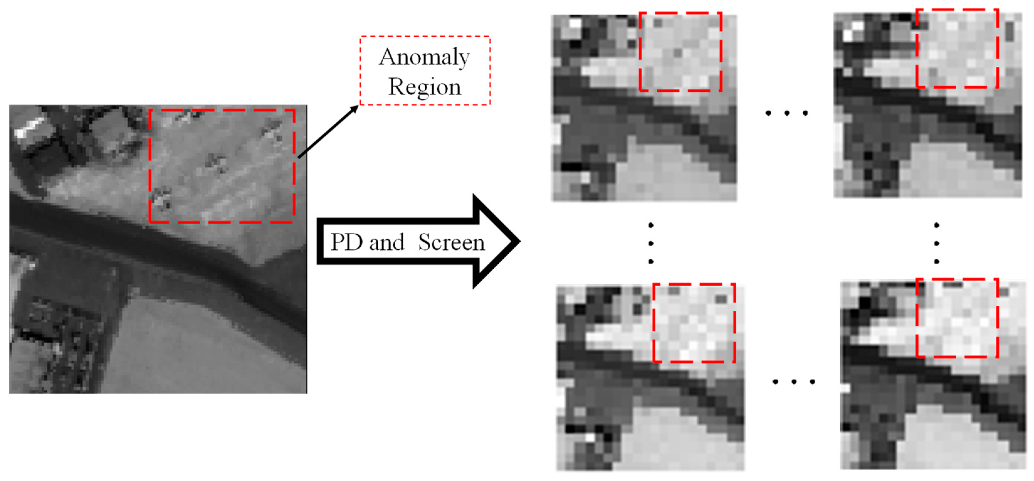
- Pixel-shuffle Down-Sampling: The primary objective of the operation is to disrupt the spatial correlation among anomalies while preserving the spatial correlation among backgrounds as much as possible, thereby enhancing the distinction between backgrounds and anomalies. Since all HSI obtained after operation exhibited remarkably strong correlations, this enabled us to train with only partial samples. Figure 3 illustrates the and diagram with a step factor of 2. In the visualization, the blue box signifies the sampling box with a step factor of 2, and each number inside represents the index of the pixel. We can intuitively see the basic process of and , A given HSI , where , , and are the row number, column number, and spectral dimension (the number of spectral channels) of the HSI, respectively, which is decomposed into four sub-images referred to as (·), and the four sub-images are recovered into an HSI referred to as . In these sub-images obtained through the operation, the scale of the anomaly target is effectively reduced in the original anomaly region. However, due to the inherent characteristics of this process, it is challenging to determine whether this region is sampled as abnormal or background pixels, and which is more dominant.
- (2)
- Spatial–Spectral Joint Screening: Samples are selected based on their spatial and spectral characteristics. The classical GRX method is utilized to obtain the spectral distribution deviation score, which indicates the degree of deviation from the background distribution. A lower score implies fewer pixels in the sample deviate from the background distribution. We aim to obtain samples with an overall minimum deviation in pixel distribution. The overall bias score on spectral characteristics can be expressed as follows:where is the stride factor for down-sampling, is the ith spectral vector in the down-sampled sample hyperspectral samples and are the mean and the covariance matrix , respectively.
2.3. Training Stage
- (1)
- Multi-Scale Mask Convolution Module (MMCM): Currently, there are two main methods for constructing blind spots. One approach uses masking to directly obscure input samples. For instance, as described in the literature [47], masking is used to obscure highly mixed areas, allowing the network to focus on learning the mapping relationship between endmembers and relatively pure region abundances. This reduces noise and yields more accurate unmixing results. The other approach employs central mask convolution, where blind spots are constructed using sliding central mask convolutions. The former requires preprocessing steps like clustering to identify candidate blind-spot regions, while the latter can adaptively construct blind spots through convolution. Therefore, we adopt the second approach and design a multi-scale mask convolution module to detect anomaly targets at different scales. Due to the characteristics of the blind-spot network, the center pixel is reconstructed based on surrounding pixel information. Therefore, we utilize small-scale mask convolution to mask the small target in the center and large-scale mask convolution to isolate similar anomalous pixels around the large target. As illustrated in Figure 1, the multi-scale mask convolution module comprises a 1 × 1 × B × 128 convolution and six mask convolutions of varying scales, with inner and outer window sizes being (1,3), (1,5), (1,7), (3,5), (3,7), and (3,9), respectively. These mask convolutions consist of two scales for an inner window and different-sized background acceptance domains for an outer window. Given training sample , , we first extract features using a convolution, followed by dividing them into six branches and using background features from various receiving fields to reconstruct obscured center pixels. The output channel is turned to 64 after the mask convolution module. Due to the varying center masks of different scale mask convolutions, their detection performance for abnormal objects also varies significantly. Small-scale mask convolutions are more suitable for detecting small targets, while large-scale mask convolutions are better suited for detecting large targets.
- (2)
- Spatial–Spectral Joint Module (SSJM): To enhance the utilization rate of spatial information and the interaction between spatial information and spectral information, we propose a spatial–spectral joint module (shown in Figure 5) that leverages deep convolution () for extracting features from different frequency bands. Additionally, deep extended convolution () is employed to capture background features at greater distances, aiding in the reconstruction of the center pixel. On the other branch, is utilized to determine the importance of various band features. These important values are then transformed into weighted enhancement features with significant contributions using a sigmoid activation function. By focusing on the most influential features, redundancy in spectral characteristics can be reduced while improving the utilization of spatial attributes. Finally, point convolution () is applied to enhance the interaction between spatial and spectral features. To prevent focus polarization caused by self-supervision, a feature fusion approach employing a jumping mode is adopted. SSJM can effectively facilitate the interaction of spatial information across different bands. The entire process can be summarized as follows:where is the feature extracted by the multi-scale mask convolution module, and is the enhanced feature by the spatial–spectral joint module.
- (3)
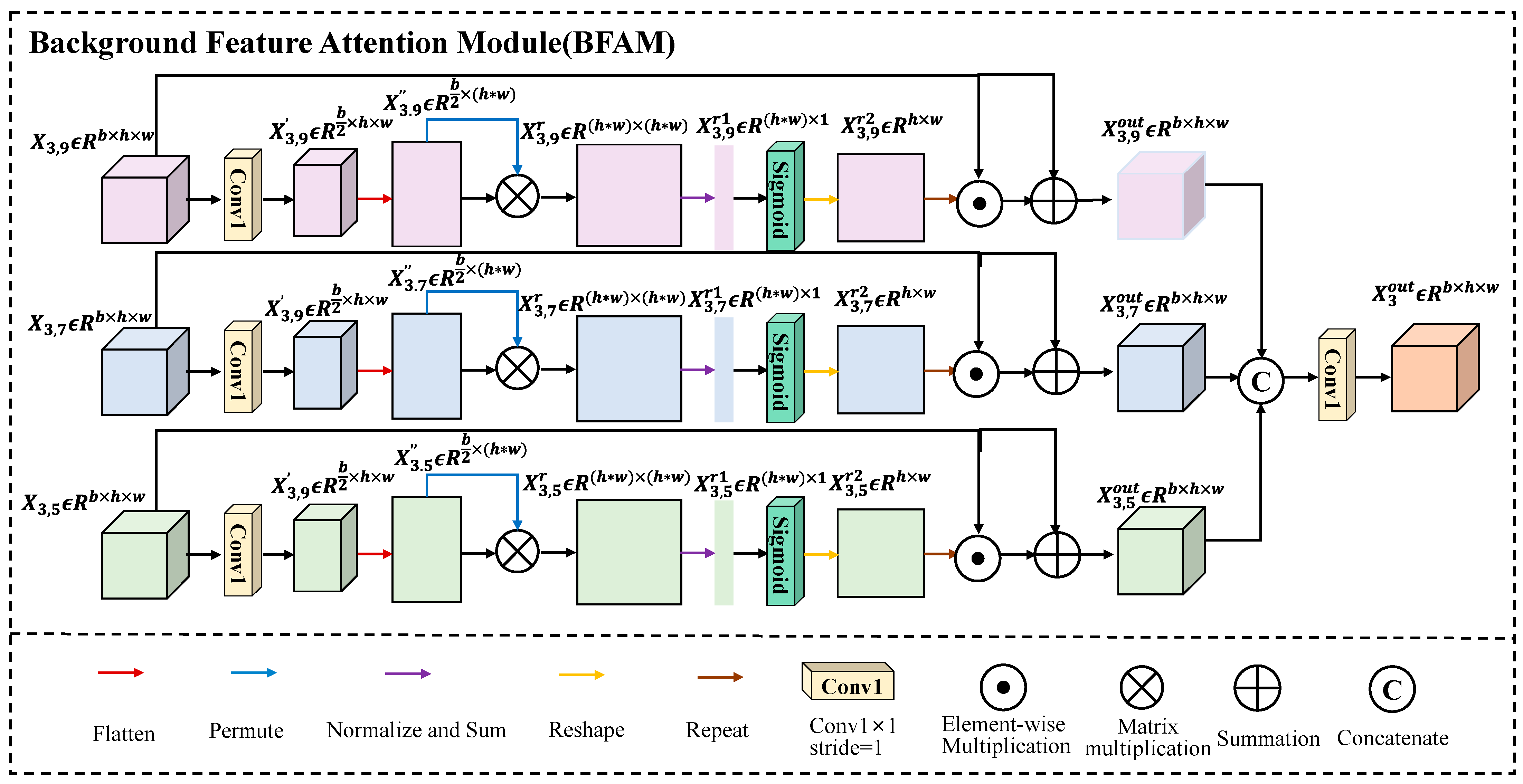
- Background Feature Attention Module (BFAM): The function of the background feature attention mechanism is to solve the problem that the mask convolution of the large background receptive field may introduce adjacent anomaly features. We need to make the network pay more attention to the background features so as to ignore the small number of introduced abnormal features. The fundamental concept involves computing the similarity between a feature vector at a specific position and other feature vectors, summing all these cosine similarities, and subsequently obtaining the confidence level for background features through a sigmoid layer. Since background accounts for most of the HSI, the background feature vector has a large similarity with other background feature vectors, while the anomaly feature is just the opposite. Finally, we obtain the background confidence of each position, which is weighted to the input feature to enhance the expression of the background feature. To prevent information loss due to extreme cases of attention, I also added a skip connection. The specific implementation process is illustrated in Figure 6. As shown in Figure 6, the features extracted by the masked convolution with the same scale but different background receptive fields are first dimensionally reduced using a convolution, which reduces the number of channels to half, thereby decreasing the computational load. Subsequently, next, channel transformations are applied, and matrix multiplication is performed to compute the dot product between the feature vector at each position and those at all other positions. This result is then normalized to obtain cosine similarity. The cosine similarities are summed row-wise to get the total similarity for each position with all other positions, and then mapped to background feature confidence using a sigmoid layer. Finally, the enhanced features are obtained by weighting the input features, and background-enhanced features are fused from the enhanced features of the three background receptive fields. Figure 6 shows the process of background feature enhancement extracted by mask convolution with an inner window of 3. It can be expressed as:where and are the eigenmatrix and the transpose of the eigenmatrix, respectively, and is the matrix multiplication. represents the inner product of spectral vectors at the positions with spectral vectors at the other positions, respectively, and
- (4)
- Dynamic Learnable Fusion Module (DLFM): The detection performance of mask convolution varies at different scales. Small-scale mask convolution exhibits good detection performance for small anomalous targets, but its performance is degraded when detecting large anomalous targets due to the interference from neighboring anomalous pixels. Conversely, the large-scale mask mold incorporates a well-designed center shielding window and demonstrates excellent detection performance for large anomaly targets. However, excessive center shielding hinders the utilization of background information in the surrounding area, making it challenging to detect smaller anomaly targets. To address multi-scale anomaly target detection requirements, we propose a dynamic learnable fusion module as shown in Figure 7. Specifically, small-scale mask convolution effectively identifies small-scale anomalous targets and reconstructs large-scale ones. On the other hand, large-scale mask convolution efficiently detects large-scale anomalous targets and reconstructs small-scale ones. Therefore, we introduce three dynamic learnable parameters , and to fuse advantages of mask convolutions at different scales, represents the weight of the feature extracted by the mask convolution with a mask window of 1, represents the weight of the feature extracted by the mask convolution with a mask window of 3, and represents the weight of the difference feature . The features extracted by the first two mask convolutions are weighted and summed, and then the weighted difference features are subtracted. Finally, the resulting features undergo dynamic weight learning and adaptation to obtain the final fused features, which enhance the background and suppress anomalies. The dynamic fusion process can be expressed as:where is the feature extracted by small-scale masked convolution, is the feature extracted by large-scale masked convolution and is the output of DLFM.
2.4. Detection Stage
| Algorithm 1 Proposed MMBSN for HAD |
| Input: the original HSI Parameters: epochs, learning rate , stride factor , Screening ratio Output: final detection result: Stage 1: Sample Preparation Stage Obtain candidate samples by PD operation Obtain training samples by spatial–spectral joint screening Stage 2: Training Stage Initialize the network with random weights for each epoch do: MMBSN update MMCM, SSJM, BFAM and DLFM by back-propagate to change MMCM, SSJM, BFAM and DLFM end Stage 3: Detection Stage Obtain the test samples by PD operation Obtain the reconstructed samples by feeding test samples into the well-trained MMBSN Obtain the reconstructed HSI by PD inverse operation Calculate the degree of anomaly for each pixel in X by (Equation (15)) |
3. Experiments and Analysis
3.1. Datasets
3.2. Evaluation Metrics
3.3. Comparison Algorithms and Evaluation Metrics
- (1)
- Comparison Algorithms: The comparison algorithms employed in the experiment encompass four conventional methods (GRX [13], FRFE [48], CRD [17], and LRASR [51]) as well as five deep learning-based approaches (GAED [38], RGAE [39], Auto-AD [40], PDBSNet [44], and BockNet [45]). GRX and FRFE are typical statistical-based methods, with FRFE being an improved version of GRX that extends traditional statistical modeling to the frequency domain. CRD and LRASR are classical representation-based methods that encompass collaborative representation, sparse representation, and low-rank representation. GAED and RGAE are early pixel-wise reconstruction deep learning methods. Auto-AD is the earliest fully convolutional hyperspectral anomaly detection network, while PDBSNet and BockNet are the latest hyperspectral anomaly detection networks using blind-spot networks. Our selection of comparison methods covers almost all existing approaches comprehensively and includes mainstream methods from different periods, which effectively highlights the validity of our comparisons. It is noteworthy that both PDBSNet and BockNet are devised based on the blind-spot network architecture, which aligns with our proposed MMBSN anomaly detection network model. Henceforth, meticulous attention should be paid to discerning disparities in the detection outcomes of these three techniques to accentuate the advantages of MMBSN. All algorithms were executed on a computer equipped with an Intel Core i7-12700H CPU, 16 GB RAM, along with GeForce RTX 3090, utilizing MATLAB 2018a and Python 3.8.18 alongside Pytorch 1.7.1 and CUDA 11.0.
- (2)
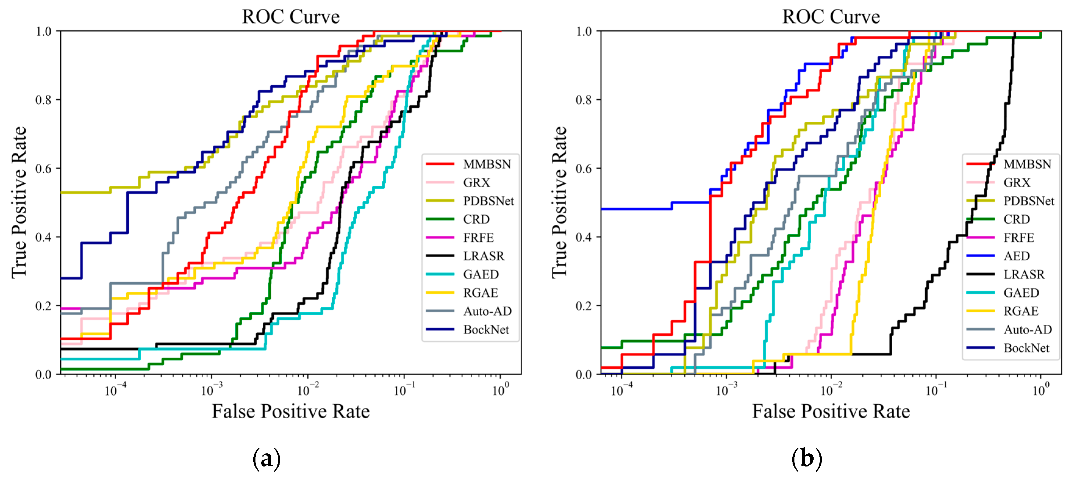
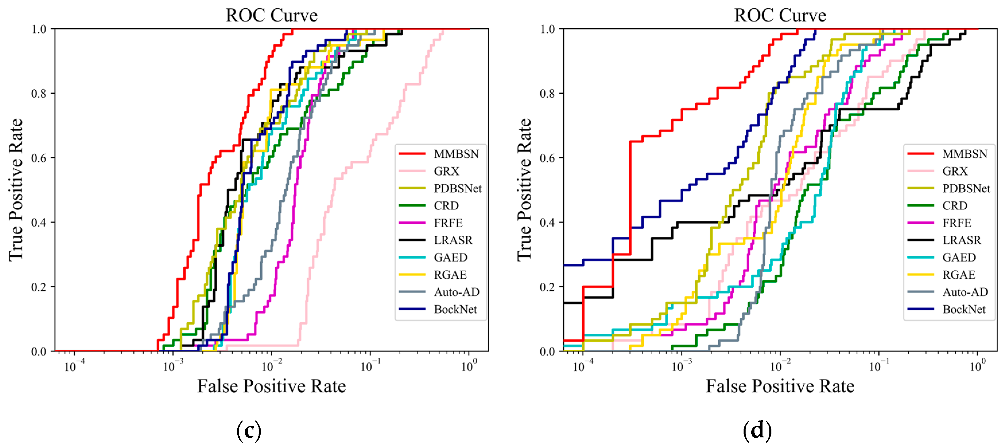
- Evaluation Metrics: In our experiments, the widely adopted HAD criteria were utilized to assess the detection performance of various methods. Specifically, we employed statistical separability map [48] and receiver operating characteristic (ROC) [51] analysis, including the area under the ROC curve (AUC) [52], as evaluation metrics. The ROC curve effectively visualizes the relationship between detection rate and false alarm rate for different methods, while the AUC quantitatively measures their detection accuracy. We anticipate a high detection rate and a low false alarm rate from the detector. Therefore, closer proximity of the ROC curve to the upper left corner and an AUC value approaching 1 indicate superior performance of the respective algorithm. Furthermore, statistical analysis can reveal differences in background suppression and anomaly separation capabilities among different methods, where the blue box represents background and the red box represents anomalies. each with a statistical range of 10–90%. Naturally, if the algorithm has a predominant ability to suppress backgrounds and separate anomalies, the blue box will be at the bottom and narrow in width, with a large gap from the red box.
3.4. Detection Performance for Different Methods
3.5. Validation
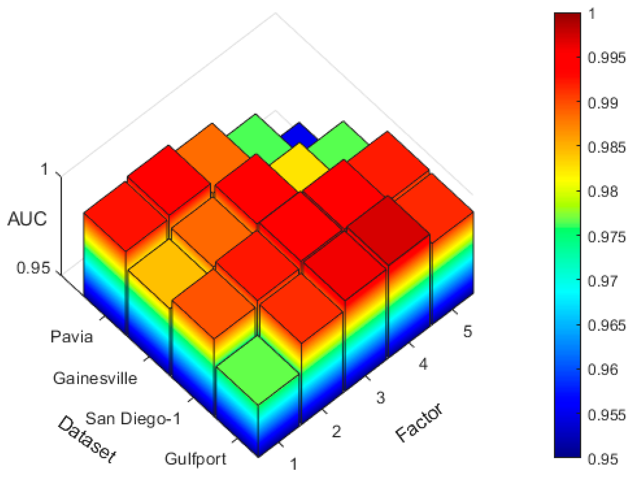
3.6. Parameter Analysis
3.7. Ablation Study
3.8. Mask Convolution Scale Characteristic Experiment
3.9. Comparison of Inference Times
4. Conclusions and Perspectives
Author Contributions
Funding
Data Availability Statement
Conflicts of Interest
References
- Sun, X.; Qu, Y.; Gao, L.; Sun, X.; Qi, H.; Zhang, B.; Shen, T. Target detection through tree-structured encoding for hyperspectral images. IEEE Trans. Geosci. Remote Sens. 2020, 59, 4233–4249. [Google Scholar] [CrossRef]
- Gao, L.; Sun, X.; Sun, X.; Zhuang, L.; Du, Q.; Zhang, B. Hyperspectral anomaly detection based on chessboard topology. IEEE Trans. Geosci. Remote Sens. 2023, 61, 5505016. [Google Scholar] [CrossRef]
- Cheng, X.; Zhang, M.; Lin, S.; Zhou, K.; Zhao, S.; Wang, H. Two-stream isolation forest based on deep features for hyperspectral anomaly detection. IEEE Geosci. Remote Sens. Lett. 2023, 20, 3271899. [Google Scholar] [CrossRef]
- Zhang, M.; Zhang, R.; Yang, Y.; Bai, H.; Zhang, J.; Guo, J. ISNet: Shape matters for infrared small target detection. In Proceedings of the IEEE/CVF Conference on Computer Vision and Pattern Recognition, New Orleans, LA, USA, 18–24 June 2022; pp. 877–886. [Google Scholar]
- Zhang, M.; Bai, H.; Zhang, J.; Zhang, R.; Wang, C.; Guo, J.; Gao, X. Rkformer: Runge-kutta transformer with random-connection attention for infrared small target detection. In Proceedings of the 30th ACM International Conference on Multimedia, Lisboa, Portugal, 10–14 October 2022; pp. 1730–1738. [Google Scholar]
- Zhang, M.; Yue, K.; Zhang, J.; Li, Y.; Gao, X. Exploring feature compensation and cross-level correlation for infrared small target detection. In Proceedings of the 30th ACM International Conference on Multimedia, Lisboa, Portugal, 10–14 October 2022; pp. 1857–1865. [Google Scholar]
- Zhang, M.; Zhang, R.; Zhang, J.; Guo, J.; Li, Y.; Gao, X. Dim2Clear Network for Infrared Small Target Detection. IEEE Trans. Geosci. Remote Sens. 2023, 61, 3263848. [Google Scholar] [CrossRef]
- Zhang, M.; Li, B.; Wang, T.; Bai, H.; Yue, K.; Li, Y. Chfnet: Curvature half-level fusion network for single-frame infrared small target detection. Remote Sens. 2023, 15, 1573. [Google Scholar] [CrossRef]
- Zhang, M.; Yang, H.; Yue, K.; Zhang, X.; Zhu, Y.; Li, Y. Thermodynamics-Inspired Multi-Feature Network for Infrared Small Target Detection. Remote Sens. 2023, 15, 4716. [Google Scholar] [CrossRef]
- Tejasree, G.; Agilandeeswari, L. An extensive review of hyperspectral image classification and prediction: Techniques and challenges. Multimedia Tools Appl. 2024, 1–98. [Google Scholar] [CrossRef]
- Su, H.; Wu, Z.; Zhang, H.; Du, Q. Hyperspectral anomaly detection: A survey. IEEE Geosci. Remote Sens. Mag. 2021, 10, 64–90. [Google Scholar] [CrossRef]
- Racetin, I.; Krtalić, A. Systematic review of anomaly detection in hyperspectral remote sensing applications. Appl. Sci. 2021, 11, 4878. [Google Scholar] [CrossRef]
- Reed, I.S.; Yu, X. Adaptive multiple-band CFAR detection of an optical pattern with unknown spectral distribution. IEEE Trans. Acoust. Speech Signal Process. 1990, 38, 1760–1770. [Google Scholar] [CrossRef]
- Molero, J.M.; Garzon, E.M.; Garcia, I.; Plaza, A. Analysis and optimizations of global and local versions of the RX algorithm for anomaly detection in hyperspectral data. IEEE J. Sel. Top. Appl. Earth Obs. Remote Sens. 2013, 6, 801–814. [Google Scholar] [CrossRef]
- Kwon, H.; Nasrabadi, N.M. Kernel RX-algorithm: A nonlinear anomaly detector for hyperspectral imagery. IEEE Trans. Geosci. Remote Sens. 2005, 43, 388–397. [Google Scholar] [CrossRef]
- Schaum, A. Joint subspace detection of hyperspectral targets. In Proceedings of the 2004 IEEE Aerospace Conference Proceedings (IEEE Cat. No. 04TH8720), Big Sky, MT, USA, 6–13 March 2004. [Google Scholar]
- Li, W.; Du, Q. Collaborative representation for hyperspectral anomaly detection. IEEE Trans. Geosci. Remote Sens. 2014, 53, 1463–1474. [Google Scholar] [CrossRef]
- Tu, B.; Li, N.; Liao, Z.; Ou, X.; Zhang, G. Hyperspectral anomaly detection via spatial density background purification. Remote Sens. 2019, 11, 2618. [Google Scholar] [CrossRef]
- Vafadar, M.; Ghassemian, H. Anomaly detection of hyperspectral imagery using modified collaborative representation. IEEE Geosci. Remote Sens. Lett. 2018, 15, 577–581. [Google Scholar] [CrossRef]
- Ling, Q.; Guo, Y.; Lin, Z.; An, W. A constrained sparse representation model for hyperspectral anomaly detection. IEEE Trans. Geosci. Remote Sens. 2018, 57, 2358–2371. [Google Scholar] [CrossRef]
- Ren, L.; Ma, Z.; Bovolo, F.; Bruzzone, L. A nonconvex framework for sparse unmixing incorporating the group structure of the spectral library. IEEE Trans. Geosci. Remote Sens. 2021, 60, 3081101. [Google Scholar] [CrossRef]
- Yuan, Y.; Ma, D.; Wang, Q. Hyperspectral anomaly detection via sparse dictionary learning method of capped norm. IEEE Access 2019, 7, 16132–16144. [Google Scholar] [CrossRef]
- Zhuang, L.; Ng, M.K.; Liu, Y. Cross-track illumination correction for hyperspectral pushbroom sensor images using low-rank and sparse representations. IEEE Trans. Geosci. Remote Sens. 2023, 61, 3236818. [Google Scholar] [CrossRef]
- Cheng, T.; Wang, B. Graph and total variation regularized low-rank representation for hyperspectral anomaly detection. IEEE Trans. Geosci. Remote Sens. 2019, 58, 391–406. [Google Scholar] [CrossRef]
- Yang, Y.; Zhang, J.; Song, S.; Liu, D. Hyperspectral anomaly detection via dictionary construction-based low-rank representation and adaptive weighting. Remote Sens. 2019, 11, 192. [Google Scholar] [CrossRef]
- Qu, Y.; Wang, W.; Guo, R.; Ayhan, B.; Kwan, C.; Vance, S.; Qi, H. Hyperspectral anomaly detection through spectral unmixing and dictionary-based low-rank decomposition. IEEE Trans. Geosci. Remote Sens. 2018, 56, 4391–4405. [Google Scholar] [CrossRef]
- Cheng, X.; Mu, R.; Lin, S.; Zhang, M.; Wang, H. Hyperspectral Anomaly Detection via Low-Rank Representation with Dual Graph Regularizations and Adaptive Dictionary. Remote Sens. 2024, 16, 1837. [Google Scholar] [CrossRef]
- Zhang, C.; Su, H.; Wang, X.; Wu, Z.; Yang, Y.; Xue, Z.; Du, Q. Self-paced Probabilistic Collaborative Representation for Anomaly Detection of Hyperspectral Images. IEEE Trans. Geosci. Remote Sens. 2024, 62, 3393303. [Google Scholar] [CrossRef]
- Kang, X.; Zhang, X.; Li, S.; Li, K.; Li, J.; Benediktsson, J.A. Hyperspectral anomaly detection with attribute and edge-preserving filters. IEEE Trans. Geosci. Remote Sens. 2017, 55, 5600–5611. [Google Scholar] [CrossRef]
- Xie, W.; Jiang, T.; Li, Y.; Jia, X.; Lei, J. Structure tensor and guided filtering-based algorithm for hyperspectral anomaly detection. IEEE Trans. Geosci. Remote Sens. 2019, 57, 4218–4230. [Google Scholar] [CrossRef]
- Wang, Z.; Wang, X.; Tan, K.; Han, B.; Ding, J.; Liu, Z. Hyperspectral anomaly detection based on variational background inference and generative adversarial network. Pattern Recognit. 2023, 143, 109795. [Google Scholar] [CrossRef]
- Zhang, S.; Meng, X.; Liu, Q.; Yang, G.; Sun, W. Feature-Decision Level Collaborative Fusion Network for Hyperspectral and LiDAR Classification. Remote Sens. 2023, 15, 4148. [Google Scholar] [CrossRef]
- Cheng, X.; Huo, Y.; Lin, S.; Dong, Y.; Zhao, S.; Zhang, M.; Wang, H. Deep Feature Aggregation Network for Hyperspectral Anomaly Detection. IEEE Trans. Instrum. Meas. 2024, 2024, 3403211. [Google Scholar] [CrossRef]
- Xiang, P.; Ali, S.; Zhang, J.; Jung, S.K.; Zhou, H. Pixel-associated autoencoder for hyperspectral anomaly detection. Int. J. Appl. Earth Obs. Geoinf. 2024, 129, 103816. [Google Scholar] [CrossRef]
- Wang, D.; Zhuang, L.; Gao, L.; Sun, X.; Zhao, X.; Plaza, A. Sliding Dual-Window-Inspired Reconstruction Network for Hyperspectral Anomaly Detection. IEEE Trans. Instrum. Meas. 2024, 62, 3351179. [Google Scholar] [CrossRef]
- Lian, J.; Wang, L.; Sun, H.; Huang, H. GT-HAD: Gated Transformer for Hyperspectral Anomaly Detection. IEEE Trans. Neural Networks Learn. Syst. 2024, 2024, 3355166. [Google Scholar] [CrossRef]
- Jiang, T.; Li, Y.; Xie, W.; Du, Q. Discriminative reconstruction constrained generative adversarial network for hyperspectral anomaly detection. IEEE Trans. Geosci. Remote Sens. 2020, 58, 4666–4679. [Google Scholar] [CrossRef]
- Xiang, P.; Ali, S.; Jung, S.K.; Zhou, H. Hyperspectral anomaly detection with guided autoencoder. IEEE Trans. Geosci. Remote Sens. 2022, 60, 3207165. [Google Scholar] [CrossRef]
- Fan, G.; Ma, Y.; Mei, X.; Fan, F.; Huang, J.; Ma, J. Hyperspectral anomaly detection with robust graph autoencoders. IEEE Trans. Geosci. Remote Sens. 2021, 60, 3097097. [Google Scholar]
- Wang, S.; Wang, X.; Zhang, L.; Zhong, Y. Auto-AD: Autonomous hyperspectral anomaly detection network based on fully convolutional autoencoder. IEEE Trans. Geosci. Remote Sens. 2021, 60, 3057721. [Google Scholar] [CrossRef]
- Wang, S.; Wang, X.; Zhang, L.; Zhong, Y. Deep low-rank prior for hyperspectral anomaly detection. IEEE Trans. Geosci. Remote Sens. 2022, 60, 3165833. [Google Scholar] [CrossRef]
- Cheng, X.; Zhang, M.; Lin, S.; Li, Y.; Wang, H. Deep Self-Representation Learning Framework for Hyperspectral Anomaly Detection. IEEE Trans. Instrum. Meas. 2023, 73, 3330225. [Google Scholar] [CrossRef]
- Wang, L.; Wang, X.; Vizziello, A.; Gamba, P. RSAAE: Residual self-attention-based autoencoder for hyperspectral anomaly detection. IEEE Trans. Geosci. Remote Sens. 2023, 61, 3271719. [Google Scholar] [CrossRef]
- Wang, D.; Zhuang, L.; Gao, L.; Sun, X.; Huang, M.; Plaza, A. PDBSNet: Pixel-shuffle down-sampling blind-spot reconstruction network for hyperspectral anomaly detection. IEEE Trans. Geosci. Remote Sens. 2023, 61, 5511914. [Google Scholar] [CrossRef]
- Wang, D.; Zhuang, L.; Gao, L.; Sun, X.; Huang, M.; Plaza, A. BockNet: Blind-block reconstruction network with a guard window for hyperspectral anomaly detection. IEEE Trans. Geosci. Remote Sens. 2023, 61, 3335484. [Google Scholar] [CrossRef]
- Gao, L.; Wang, D.; Zhuang, L.; Sun, X.; Huang, M.; Plaza, A. BS 3 LNet: A new blind-spot self-supervised learning network for hyperspectral anomaly detection. IEEE Trans. Geosci. Remote Sens. 2023, 61, 3246565. [Google Scholar]
- Xu, M.; Xu, J.; Liu, S.; Sheng, H.; Yang, Z. Multi-Scale Convolutional Mask Network for Hyperspectral Unmixing. IEEE J. Sel. Top. Appl. Earth Obs. Remote Sens. 2024, 17, 3687–3700. [Google Scholar] [CrossRef]
- Manolakis, D.; Shaw, G. Detection algorithms for hyperspectral imaging applications. IEEE Signal Process. Mag. 2002, 19, 29–43. [Google Scholar] [CrossRef]
- Bradley, A.P. The use of the area under the ROC curve in the evaluation of machine learning algorithms. Pattern Recognit. 1997, 30, 1145–1159. [Google Scholar] [CrossRef]
- Ferri, C.; Hernández-Orallo, J.; Flach, P.A. A coherent interpretation of AUC as a measure of aggregated classification performance. In Proceedings of the 28th International Conference on Machine Learning (ICML-11), Bellevue, WA, USA, 28 June–2 July 2011; pp. 657–664. [Google Scholar]
- Xu, Y.; Wu, Z.; Li, J.; Plaza, A.; Wei, Z. Anomaly detection in hyperspectral images based on low-rank and sparse representation. IEEE Trans. Geosci. Remote Sens. 2015, 54, 1990–2000. [Google Scholar] [CrossRef]
- Chang, C.-I. An effective evaluation tool for hyperspectral target detection: 3D receiver operating characteristic curve analysis. IEEE Trans. Geosci. Remote Sens. 2020, 59, 5131–5153. [Google Scholar] [CrossRef]
- Xiao, S.; Zhang, T.; Xu, Z.; Qu, J.; Hou, S.; Dong, W. Anomaly detection of hyperspectral images based on transformer with spatial–spectral dual-window mask. IEEE J. Sel. Top. Appl. Earth Obs. Remote Sens. 2023, 16, 1414–1426. [Google Scholar] [CrossRef]


| Dataset | Sensor | Image Size | Resolution |
|---|---|---|---|
| Pavia | ROSIS | 150 × 150 × 102 | 1.3 m |
| Gainesville | AVIRIS | 100 × 100 × 191 | 3.5 m |
| San Diego | AVIRIS | 100 × 100 × 189 | 3.5 m |
| Gulfport | AVIRIS | 100 × 100 × 191 | 3.4 m |
| Dataset | of Different Methods | |||||||||
|---|---|---|---|---|---|---|---|---|---|---|
| GRX | FRFE | CRD | LRASR | GAED | RGAE | Auto-AD | PDBSNet | BockNet | MMBSN | |
| Pavia | 0.9538 | 0.9457 | 0.9510 | 0.9380 | 0.9398 | 0.9688 | 0.9925 | 0.9915 | 0.9905 | 0.9945 1 |
| Gainesville | 0.9684 | 0.9633 | 0.9536 | 0.7283 | 0.9829 | 0.9647 | 0.9808 | 0.9863 | 0.9901 | 0.9963 1 |
| San Diego | 0.8736 | 0.9787 | 0.9768 | 0.9824 | 0.9861 | 0.9854 | 0.9794 | 0.9892 | 0.9901 | 0.9961 1 |
| Gulfport | 0.9526 | 0.9722 | 0.9342 | 0.9120 | 0.9705 | 0.9842 | 0.9825 | 0.9895 | 0.9955 | 0.9983 1 |
| Average | 0.9371 | 0.9650 | 0.9539 | 0.8902 | 0.9698 | 0.9758 | 0.9838 | 0.9891 | 0.9916 | 0.9963 1 |
| Factor | The AUC of Different Factors on Four Datasets | |||
|---|---|---|---|---|
| Pavia | Gainesville | San Diego | Gulfport | |
| 1 (Rate = 1.0) | 0.9925 | 0.9842 | 0.9896 | 0.9767 |
| 2 (Rate = 0.5) | 0.9941 | 0.9886 | 0.9923 | 0.9913 |
| 3 (Rate = 0.5) | 0.9884 | 0.9936 | 0.9953 | 0.9960 |
| 4 (Rate = 0.5) | 0.9763 | 0.9826 | 0.9947 | 0.9971 |
| 5 (Rate = 0.5) | 0.9552 | 0.9765 | 0.9921 | 0.9915 |
| Rate | The AUC of Different Rates on Four Datasets | |||
|---|---|---|---|---|
| Pavia (Factor = 2) | Gainesville (Factor = 3) | San Diego (Factor = 3) | Gulfport (Factor = 4) | |
| 0.1 | 0.9920 | 0.9881 | 0.9928 | 0.9945 |
| 0.2 | 0.9920 | 0.9881 | 0.9928 | 0.9961 |
| 0.3 | 0.9920 | 0.9917 | 0.9944 | 0.9940 |
| 0.4 | 0.9920 | 0.9941 | 0.9962 | 0.9951 |
| 0.5 | 0.9938 | 0.9898 | 0.9949 | 0.9974 |
| 0.6 | 0.9938 | 0.9902 | 0.9941 | 0.9950 |
| 0.7 | 0.9938 | 0.9891 | 0.9923 | 0.9933 |
| 0.8 | 0.9906 | 0.9832 | 0.9917 | 0.9927 |
| 0.9 | 0.9906 | 0.9740 | 0.9906 | 0.9912 |
| 1.0 | 0.9882 | 0.9681 | 0.9899 | 0.9837 |
| Component | Case1 | Case2 | Case3 | Case4 | Case5 | Case6 |
|---|---|---|---|---|---|---|
| MMCM | × | √ | √ | √ | √ | √ |
| SSJM | √ | × | √ | √ | × | √ |
| BFAM | √ | √ | × | √ | √ | √ |
| DWMEB | × | × | × | × | √ | × |
| DLFM | √ | √ | √ | × | √ | √ |
| Dataset | The AUC of different cases | |||||
| Pavia | 0.9862 | 0.9923 | 0.9901 | 0.9938 | 0.9931 | 0.9943 1 |
| Gainesville | 0.9772 | 0.9920 | 0.9882 | 0.9923 | 0.9955 | 0.9960 1 |
| San Diego | 0.9820 | 0.9929 | 0.9910 | 0.9927 | 0.9944 | 0.9952 1 |
| Gulfport | 0.9667 | 0.9917 | 0.9889 | 0.9911 | 0.9961 | 0.9976 1 |
| Scale | The AUC of Different Case on Pavia and San Diego Datasets | |
|---|---|---|
| Pavia | San Diego | |
| 0.9936 | 0.9876 | |
| 0.9897 | 0.9946 | |
| ALL | 0.9945 | 0.9960 |
| Dataset | Inference Time of Different Detectors | |||||||||
|---|---|---|---|---|---|---|---|---|---|---|
| GRX | FRFE | CRD | LRASR | GAED | RGAE | Auto-AD | PDBSNet | BockNet | MMBSN | |
| Pavia | 0.9823 | 33.5833 | 5.3146 | 61.1938 | 0.1072 | 0.0476 | 0.0305 1 | 0.0419 | 0.9258 | 0.4580 2 |
| Gainesville | 0.1155 | 14.3275 | 9.9203 | 55.5105 | 0.0347 2 | 0.0608 | 0.0209 1 | 0.0270 | 0.9440 | 0.4285 |
| San Diego | 0.2146 | 9.8865 | 3.9145 | 46.3339 | 0.0305 | 0.0335 | 0.0274 2 | 0.0266 1 | 0.9594 | 0.3595 |
| Gulfport | 0.5988 | 13.6096 | 5.0287 | 63.4349 | 0.0620 | 0.0373 | 0.0220 1 | 0.0281 | 0.9238 | 0.4975 2 |
| Average | 0.4778 | 17.8517 | 6.0445 | 56.6183 | 0.0586 | 0.0448 | 0.0252 1 | 0.0309 2 | 0.9383 | 0.4359 |
Disclaimer/Publisher’s Note: The statements, opinions and data contained in all publications are solely those of the individual author(s) and contributor(s) and not of MDPI and/or the editor(s). MDPI and/or the editor(s) disclaim responsibility for any injury to people or property resulting from any ideas, methods, instructions or products referred to in the content. |
© 2024 by the authors. Licensee MDPI, Basel, Switzerland. This article is an open access article distributed under the terms and conditions of the Creative Commons Attribution (CC BY) license (https://creativecommons.org/licenses/by/4.0/).
Share and Cite
Yang, Z.; Zhao, R.; Meng, X.; Yang, G.; Sun, W.; Zhang, S.; Li, J. A Multi-Scale Mask Convolution-Based Blind-Spot Network for Hyperspectral Anomaly Detection. Remote Sens. 2024, 16, 3036. https://doi.org/10.3390/rs16163036
Yang Z, Zhao R, Meng X, Yang G, Sun W, Zhang S, Li J. A Multi-Scale Mask Convolution-Based Blind-Spot Network for Hyperspectral Anomaly Detection. Remote Sensing. 2024; 16(16):3036. https://doi.org/10.3390/rs16163036
Chicago/Turabian StyleYang, Zhiwei, Rui Zhao, Xiangchao Meng, Gang Yang, Weiwei Sun, Shenfu Zhang, and Jinghui Li. 2024. "A Multi-Scale Mask Convolution-Based Blind-Spot Network for Hyperspectral Anomaly Detection" Remote Sensing 16, no. 16: 3036. https://doi.org/10.3390/rs16163036
APA StyleYang, Z., Zhao, R., Meng, X., Yang, G., Sun, W., Zhang, S., & Li, J. (2024). A Multi-Scale Mask Convolution-Based Blind-Spot Network for Hyperspectral Anomaly Detection. Remote Sensing, 16(16), 3036. https://doi.org/10.3390/rs16163036