Rational Polynomial Coefficient Estimation via Adaptive Sparse PCA-Based Method

Abstract

The Rational Function Model (RFM) is composed of numerous highly correlated Rational Polynomial Coefficients (RPCs), establishing a mathematical relationship between two-dimensional images and three-dimensional spatial coordinates. Due to the existence of ill-posedness and overparameterization, the estimated RPCs are sensitive to any slight perturbations in the observation data, particularly when handling a limited number of Ground Control Points (GCPs). Recently, Principal Component Analysis (PCA) has demonstrated significant performance improvements in the RFM optimization problem. In the PCA-based RFM, each Principal Component (PC) is a linear combination of all variables in the design matrix. However, some original variables are noise related and have very small or almost zero contributions to the construction of PCs, which leads to the overparameterization problem and makes the RPC estimation process ill posed. To address this problem, in this paper, we propose an Adaptive Sparse Principal Component Analysis-based RFM method (ASPCA-RFM) for RPC estimation. In this method, the Elastic Net sparsity constraint is introduced to ensure that each PC contains only a small number of original variables, which automatically eliminates unnecessary variables during PC computation. Since the optimal regularization parameters of the Elastic Net vary significantly in different scenarios, an adaptive regularization parameter approach is proposed to dynamically adjust the regularization parameters according to the explained variance of PCs and degrees of freedom. By adopting the proposed method, the noise and error in the design matrix can be reduced, and the ill-posedness and overparameterization of the RPC estimation can be significantly mitigated. Additionally, we conduct extensive experiments to validate the effectiveness of our method. Compared to existing state-of-the-art methods, the proposed method yields markedly improved or competitive performance.

1. Introduction

Optical remote sensing satellites are increasingly required and utilized in a wide range of applications, such as digital map generation, space surveillance, meteorological monitoring and disaster early warning [1]. To extract accurate spatial information from remote sensing images, two categories of sensor models are used to represent the mathematical relationship between image and ground spaces: rigorous models and generic models [2]. Rigorous models simulate the physical imaging process of satellite sensors; hence, they are extremely complex and require ephemeris, attitude and other ancillary data from the satellite platform [3,4]. However, the Rational Function Model (RFM), as the most popular generic model, is independent of satellite sensors and provides a mathematically simple and straightforward approach to describe the geometric mapping from the three-dimensional world to the corresponding two-dimensional image coordinate system [5].

The RFM is the ratio of two cubic polynomials with 80 Rational Polynomial Coefficients (RPCs). The estimation of RPCs is accomplished through a regression algorithm using a series of Ground Control Points (GCPs) that is composed of geographic coordinates (i.e., latitude, longitude and height) and corresponding image coordinates (i.e., line and sample). Nevertheless, the existence of a large number of highly correlated RPCs makes the estimation essentially an ill-posed problem [5]. Due to the multicollinearity of the design matrix, a small amount of noise or errors in the observation data may significantly affect the estimated RPCs [6]. This paper aims to address the problems of ill-posedness and overparameterization during the RPC estimation process, especially when the number of the observation data is insufficient.

Previous studies related to RPC estimation can be roughly divided into two types: regularization-based methods [7,8,9,10] and variable selection methods [11,12,13,14,15,16]. The first type involves finding optimal results through parameter penalties during the optimization process. Ridge estimation is a member of the first group of regularization-based techniques that computes RPCs by minimizing the residuals and the $l_2$-norm of the estimated parameters [7]. However, $l_2$-norm regularization does not reduce the demand for observation data. Long et al. [9] proposed an $l_1$-norm-regularized least squares (L1LS) method that applies the $l_1$-norm to parameter minimization. The L1LS method typically yields sparse results of RPCs with only a few non-zero elements, making the ill-posed problem well posed. Consequently, this method can estimate more robust RPCs with fewer Ground Control Points (GCPs). Despite the many advantages of L1LS, manually selecting an optimal value of the regularization parameter remains challenging. To address this problem, Gholinejad et al. [10] proposed a parameter-free linear framework for RFM optimization, which imposes the $l_1$-norm on both the residuals and the RPCs within the linear objective function.

The second type of method involves removing unnecessary parameters from the RPCs, known as variable selection methods. Zhao et al. [11] directly left out the third-order terms, while Zhang et al. [12] omitted redundant RPCs using a scatter matrix and elimination transformation strategy. Additionally, some well-known variable selection methods include the particle swarm optimization method [13], the nested regression-based optimal selection method [14], and the two-stage uncorrelated and statistically significant RFM (USS-RFM) [15]. To determine the optimal RPCs, Zoej et al. [16] employed a meta-heuristic optimization algorithm to search the solution space based on the root mean square error of some GCPs. In recent years, with the rapid development of satellite processing hardware, many researchers [17,18] explore the onboard processing techniques on satellite remote sensing images, especially for the implementation of RPC estimation, which focuses on the application of high-performance and disruptive computing in remote sensing, providing more technical support and research directions for the implementation of RPC solving on satellites. Furthermore, Zhang et al. [19] proposed a field-programmable gate array (FPGA)-based fixed-point (FP)-RPC orthorectification method. This method significantly improves computational speed and reduces resource consumption compared to PC-based RPC while ensuring accuracy.

As mentioned above, due to ill-posedness and overparameterization problems, any small perturbation in the observation data can significantly affect the estimated results [6]. The Principal Component Analysis-based RFM method (PCA-RFM) [20] performs variable selection in the Principal Component (PC) space, which achieves dimensionality reduction while mitigating the effect of noise. In PCA-RFM, PCs with small eigenvalues are considered noise related and can be directly discarded. PCA-RFM removes PCs with eigenvalues smaller than a preset threshold and then reconstructs the design matrix through PCA inverse transformation. Subsequently, the design matrix, with significantly reduced noise interference, allows stable RPCs to be obtained through QR decomposition and the least squares (LS) method [21]. However, selecting the optimal threshold parameter is a key factor in determining the algorithm’s performance. Therefore, based on PCA-RFM, the APCA-RFM method [6] developed the thresholding ridge ratio criterion to achieve a parameter-free RFM method. Another method with a similar mathematical representation to PCA is the Empirical Orthogonal Function and Singular Value Decomposition method (EOF-SVD), which is utilized to analyze spatio-temporal environmental data [22,23]. The EOF-SVD method combines EOF analysis and SVD techniques, focusing on extracting the main spatio-temporal patterns and variations from the data, and is commonly used in fields such as meteorology, oceanography and earth sciences.

The aforementioned PCA-based RFM methods reduced the effect of multicollinearity by discarding noise-related PCs. From the perspective of each PC, it seeks the linear combination of all original variables, with each element in the eigenvector indicating the weight of each variable in the design matrix. In RFM problems, the extraction process of GCPs inevitably introduces varying degrees of errors and noise, directly leading to the instability of variables in the design matrix. Typically, the elements in the eigenvectors are non-zero; however, some of the original variables are noise related and have very small or almost zero contributions to PC construction. Removing these unnecessary elements from the eigenvectors yields more robust regression results [24]. Based on this motivation, we introduce Sparse Principal Component Analysis (SPCA) [24] into the RPC estimation problem and propose an Adaptive Sparse PCA-RFM method (ASPCA-RFM). Even in the case of insufficient GCPs, our proposed method can ensure accurate and stable geographical information from remote sensing images.

Similarly to SPCA [24], we incorporate the Elastic Net [25] constraint into the PCA decomposition process to derive sparse eigenvectors. Through this approach, each PC consists of only a subset of the original variables in the design matrix. Additionally, each eigenvector requires an Elastic Net regression (i.e., 78 times regression operations for all PCs), which demands significant extra computational resources. To address this problem, we adopt the Non-linear Iterative Partial Least Squares (NIPALS) [26] framework to compute eigenvectors iteratively and only employed the Elastic Net constraint on signal-related PCs. Moreover, applying the Elastic Net to the eigenvectors can automatically shrink noise-related PCs to zero vectors, without the need to define a threshold parameter or employ a complex automatic threshold selection algorithm as in PCA-RFM or APCA-RFM. Furthermore, since the regularization parameter of the Elastic Net greatly determines the algorithm’s performance, we propose an adaptive regularization parameter approach to dynamically adjust the regularization parameters based on the explained variance of PCs and degrees of freedom, thereby enhancing the performance of the ASPCA-RFM method. The main contributions of this paper are three-fold:

(1)

We incorporate SPCA into the RPC estimation problem to automatically eliminate unnecessary and noise-related variables during PC computation.

(2)

We propose an adaptive regularization parameter approach to dynamically adjust the regularization parameters based on the explained variance of PCs and degrees of freedom, enhancing the method’s robustness in different scenarios.

(3)

We conduct extensive experiments to evaluate the performance of the proposed method, and the results show that our method demonstrates improved performance compared to existing competing methods.

The remainder of this paper is organized as follows. In Section 2, the RFM structure and the PCA-based RFM algorithm are introduced. In Section 3, an improved RPC estimation method based on adaptive sparse PCA is proposed. In Section 4, the performance of different competing methods is evaluated on several real datasets to verify the effectiveness of the proposed method. Finally, Section 5 presents some discussion and conclusions.

2. Theoretical Background

2.1. Rational Function Model

The RFM defines a transformation relationship between the image pixel coordinates and the ground coordinates by the ratios of polynomials. The mathematical form of the ground-to-image transformation [27] can be expressed as follows:

$$l={\displaystyle \frac{N_l(X,Y,Z)}{D_l(X,Y,Z)}}$$

(1)

$$s={\displaystyle \frac{N_s(X,Y,Z)}{D_s(X,Y,Z)}}$$

(2)

where $(l,s)$ represents normalized line and sample coordinates in the image space. $(X,Y,Z)$ represents normalized coordinates of ground points in Earth space. $N_l$, $D_l$, $N_s$ and $D_s$ denote four third-order polynomial functions, given by the following equations.

$$\begin{array}{c}{N}_l(X,Y,Z)=a_1+a_{2}X+a_{3}Y+\cdots +a_{20}{Z}^3\hfill \\ D_l(X,Y,Z)=b_1+b_{2}X+b_{3}Y+\cdots +b_{20}{Z}^3\hfill \\ N_s(X,Y,Z)=c_1+c_{2}X+c_{3}Y+\cdots +c_{20}{Z}^3\hfill \\ D_s(X,Y,Z)=d_1+d_{2}X+d_{3}Y+\cdots +d_{20}{Z}^3\hfill \end{array}$$

(3)

where $a_i$, $b_i$, $c_i$, $d_i$ (i = 1, 2, ⋯, 20) are Rational Polynomial Coefficients. Although the RFM is a nonlinear model, it is usually expressed as a linear form by setting $b_1$ and $d_1$ to 1. When $b_1$ and $d_1$ are not equal to 1, each line and sample coefficients can be divided by $b_1$ and $d_1$, respectively, to obtain a linear form of RFM, as follows:

$$\begin{array}{c}{N}_l(X,Y,Z)-l·D_l(X,Y,Z)=0\hfill \\ N_s(X,Y,Z)-s·D_s(X,Y,Z)=0\hfill \end{array}$$

(4)

In order to estimate the RPCs, the above equations can be reformulated as a standard linear Gauss–Markov model [9]:

$$\mathbf{y}=\mathbf{Ax}+\mathbf{e}$$

(5)

where $\mathbf{y}\in {\mathbf{R}}^{2n}$ is the vector of observations, $\mathbf{A}\in {\mathbf{R}}^{2n\times r}$ is the design matrix, $\mathbf{x}\in {\mathbf{R}}^r$ is the vector of unknowns (i.e., RPCs) and $\mathbf{e}\in {\mathbf{R}}^{2n}$ is the vector of random errors. In this case, n always represents the number of GCPs and r is set to 78 which is the number of the unknown RPCs. Thus, the observation equations and design matrix can be written as follows:

$$\mathbf{A}={\left[\begin{array}{cc}{\mathbf{A}}_l& \mathbf{0}\\ \mathbf{0}& {\mathbf{A}}_s\end{array}\right]}_{2n\times r}$$

(6)

where ${\mathbf{A}}_l\in {\mathbf{R}}^{n\times 39}$ and ${\mathbf{A}}_s\in {\mathbf{R}}^{n\times 39}$ are the design matrices of lines and samples, respectively, which can be formulated as follows:

$$\begin{array}{c}{\mathbf{A}}_l={[{\mathbf{A}}_{l1},{\mathbf{A}}_{l2},\cdots ,{\mathbf{A}}_{ln}]}^T\hfill \\ {\mathbf{A}}_s={[{\mathbf{A}}_{s1},{\mathbf{A}}_{s2},\cdots ,{\mathbf{A}}_{sn}]}^T\hfill \end{array}$$

(7)

$$\begin{array}{c}{\mathbf{A}}_{li}={[1,X_i,Y_i,\cdots ,Z_i^3,-l_i{X}_i,-l_i{Y}_i,\cdots ,-l_i{Z}_i^3]}^T\hfill \\ {\mathbf{A}}_{si}={[1,X_i,Y_i,\cdots ,Z_i^3,-s_i{X}_i,-s_i{Y}_i,\cdots ,-s_i{Z}_i^3]}^T\hfill \end{array}$$

(8)

The vector of observation $\mathbf{y}$ and the vector of RPCs are defined as follows:

$$\mathbf{y}={[l_1,l_2,\cdots ,l_n,s_1,s_2,\cdots ,s_n]}^T$$

(9)

$$\begin{array}{c}\mathbf{x}=[a_1,a_2,\cdots ,a_{40},b_2,b_3,\cdots ,b_{40},c_1,c_2,\cdots ,c_{40},d_2,d_3,\cdots ,d_{40}{]}^T\hfill \end{array}$$

(10)

The standard linear Gauss–Markov model can be estimated by the Ordinary Least Squares (OLS) method [21]:

$$\hat{\mathbf{x}}={\left({\mathbf{A}}^T\mathbf{A}\right)}^{-1}{\mathbf{A}}^T\mathbf{y}$$

(11)

In Equation (6), $rank\left(\mathbf{A}\right)\le min(2n,r)$, indicating linear correlation between the column vectors of $\mathbf{A}$. These multicollinearity problems may result in the instability of the regression model and inaccuracy of the parameter estimation.

2.2. PCA-Based RFM Optimization

The measurement noise of observations (GCPs) is inevitably transmitted to the design matrix. Thus, it is efficient to apply PCA to the design matrix to obtain noise-free results. The mean-centered design matrix $\overline{\mathbf{A}}$ can be computed as follows:

$$\overline{\mathbf{A}}=\mathbf{A}-mean\left(\mathbf{A}\right)$$

(12)

Then, the covariance matrix $\mathbf{C}$ of $\overline{\mathbf{A}}$ is determined by the following equation [21]:

$$\mathbf{C}={\displaystyle \frac{{\overline{\mathbf{A}}}^T\overline{\mathbf{A}}}{n-1}}$$

(13)

After specifying $\mathbf{C}$, the PCA transformation [20] is applied to $\overline{\mathbf{A}}$, as follows:

$$\mathbf{Q}=\overline{\mathbf{A}}\mathbf{V}$$

(14)

where $\mathbf{V}$ is the matrix of eigenvectors of $\mathbf{C}$ and $\mathbf{Q}$ is a matrix containing 78 Principal Components (PCs), equal to the number of unknown RPCs. It is usually to set ${\lambda }_1,{\lambda }_2,\cdots ,{\lambda }_{78}$ as the decreasingly ordered eigenvalues of $\mathbf{C}$, and eigenvectors with larger eigenvalues are always considered as more important vectors with larger explained variance. Therefore, only the first k PCs are retained while others are discarded. Normally, the value of k is calculated by a preset threshold value, as follows:

$$k=\underset{j}{max}\left\{\left.j:{\lambda }_j>t\right\}\right.,j=1,\cdots ,78$$

(15)

where t is a preset threshold value. ${\mathbf{V}}_k$ is defined as a matrix that consists of the first k eigenvectors. When ${\mathbf{V}}_k$ is assigned, the reconstructed design matrix ${\mathbf{A}}_{re}$ is determined by the following formula [6].

$${\overline{\mathbf{A}}}_{re}=\overline{\mathbf{A}}{\mathbf{V}}_k{{\mathbf{V}}_k}^T$$

(16)

$${\mathbf{A}}_{re}={\overline{\mathbf{A}}}_{re}+mean\left(\mathbf{A}\right)$$

(17)

Finally, the noise of the design matrix is significantly reduced and the unknown RPCs can be easily computed by QR decomposition with column pivoting and the LS method [21]. Through the PCA-based RFM method, the estimated RPCs are more robust to the problems of ill-posedness and overparameterization.

3. Methodology

3.1. SPCA-Based RFM Method via NIPALS

In PCA-based RPC estimation methods, as indicated in Equation (14), each element in the eigenvector represents the weight of each variable in the design matrix. However, not all variables are necessary, and some are even noise related for the RPC estimation problem. Removing these redundant elements from the eigenvectors yields more robust regression results, particularly when the observation data are insufficient. To address this problem, we introduce the Sparse Principal Component Analysis (SPCA) method in the RFM task. SPCA can be viewed as adding a variable selection capability to PCA, determining which variables are most important for constructing PCs through sparse constraints. SPCA [24] imposes an Elastic Net constraint on the reconstruction of eigenvectors, as follows:

$${\hat{\mathbf{v}}}_i=arg\underset{{\mathbf{v}}_i}{min}{∥{\mathbf{q}}_i-\overline{\mathbf{A}}{\mathbf{v}}_i∥}_2^2+\mu \left[{\displaystyle \frac{(1-\alpha )}{2}}{∥{\mathbf{v}}_i∥}_2^2+\alpha {∥{\mathbf{v}}_i∥}_1\right]$$

(18)

where ${\hat{\mathbf{v}}}_i$ is the output of Elastic Net regression, and ${\mathbf{v}}_i$ and ${\mathbf{q}}_i$ denote the i-th eigenvector and i-th PC, respectively. The Elastic Net is essentially a combination of $l_2$-norm and $l_1$-norm [28] regularization. $\mu$ and $\alpha$ are two regularization parameters. $\alpha$ controls the balance between $l_1$ and $l_2$ penalties. When $\alpha =1$, the Elastic Net reduces to Lasso; when $\alpha =0$, it becomes ridge regression. $\mu$ is another tuning parameter that controls the overall strength of the regularization. A higher value of $\mu$ increases the penalty on the magnitude of coefficients, leading to more sparse results. SPCA introduces the Elastic Net regularization constraint in the estimation of eigenvectors, automatically setting unnecessary variables to zero when constructing the PCs. This helps to reduce the impact of unnecessary variables on the estimation of PCs and regression results. Due to the existence of severe multicollinearity and a large number of redundant variables in the design matrix, especially in the case of insufficient data, SPCA ensures that each PC consists of only a subset of the most important original variables, which significantly enhances the robustness of RPC estimation.

According to Equation (18), each eigenvector requires an Elastic Net regression operation, which is computationally inefficient. The most popular algorithms for computing PCA decomposition are Eigenvalue Decomposition (EVD) and Nonlinear Iterative Partial Least Square (NIPALS) algorithms [26]. EVD is a traditional PCA decomposition method that obtains PCs by computing the eigenvalues and eigenvectors of the covariance matrix of the data. When the full PCs are required, EVD is more numerically robust and efficient. NIPALS iteratively calculates the PCA decomposition, one PC at a time in descending order. When only several leading PCs with the largest eigenvalues are required, it is more computationally efficient to apply NIPALS algorithm. In the RFM problem, it is often necessary to calculate only a small number of PCs (e.g., 10 to 20 out of a total of 78 PCs). Therefore, to reduce computational resources in this task, we adopt the proposed method based on the NIPALS framework. The description of the SPCA-based RFM algorithm is provided in Algorithm 1.

In the NIPALS algorithm, the input is the mean-centered design matrix $\overline{\mathbf{A}}$. The matrix ${\mathbf{V}}_k\in {\mathbf{R}}^{r\times k}$ contains the first k ordered sparse eigenvectors (in descending eigenvalue order). k is the number of retained PCs. ${\mathbf{Q}}_k\in {\mathbf{R}}^{2n\times k}$ represents the geometric projection of $\overline{\mathbf{A}}$ on the columns of ${\mathbf{V}}_k$, also known as the PCs. All symbols in Algorithm 1 are the same as those in Section 2.2.

Algorithm 1 $[{\mathbf{V}}_k,{\mathbf{Q}}_k,k]=\mathrm{NIPALS}\left(\overline{\mathbf{A}}\right)$

1: Require: Mean-Centered Design Matrix $\overline{\mathbf{A}}$,   2:    Set $\mathbf{R}=\mathbf{A}$   3:    Initialize ${\mathbf{V}}_0={\mathbf{Q}}_0=\varnothing$   4:    Set $\epsilon ={10}^{-6}$ (convergence threshold)   5:    Initialize $\mathbf{q}$ to a non-zero column of $\mathbf{R}$   6:    for $j=1$ to 78 do   7:         Set ${\mathbf{q}}_{new}=\mathbf{q}$ and ${\mathbf{q}}_{old}=10\mathbf{q}$   8:         while ${∥{\mathbf{q}}_{new}-{\mathbf{q}}_{old}∥}_2>\epsilon$ do   9:             ${\mathbf{q}}_{old}={\mathbf{q}}_{new}$ 10:             $\mathbf{v}={\mathbf{R}}^T\mathbf{q}/{\mathbf{q}}^T\mathbf{q}$ 11:             $\mathbf{v}=\mathbf{v}/\sqrt{{\mathbf{v}}^T\mathbf{v}}$ 12:             $\mathbf{q}=\mathbf{Rv}$ 13:             ${\mathbf{q}}_{new}=\mathbf{q}$ 14:         end while 15:         $\hat{\mathbf{v}}=arg\underset{\mathbf{v}}{min}{∥\mathbf{q}-\overline{\mathbf{A}}\mathbf{v}∥}_2^2+\mu \left[{\displaystyle \frac{(1-\alpha )}{2}}{∥\mathbf{v}∥}_2^2+\alpha {∥\mathbf{v}∥}_1\right]$ 16:         if $\hat{\mathbf{v}}==\mathbf{0}$ 17:             $k=j-1$ 18:             break 19:         end if 20:         ${\mathbf{Q}}_j=\left[\begin{array}{cc}{\mathbf{Q}}_{j-1}& \mathbf{R}\hat{\mathbf{v}}\end{array}\right]$ 21:         ${\mathbf{V}}_j=\left[\begin{array}{cc}{\mathbf{V}}_{j-1}& \hat{\mathbf{v}}\end{array}\right]$ 22:         $\mathbf{R}=\mathbf{R}-\mathbf{q}{\mathbf{v}}^T$ 23:    end for 24:    return ${\mathbf{V}}_k$, ${\mathbf{Q}}_k$, k

NIPALS can be regarded as a variant of the power method [29], which iteratively computes each PC and then performs matrix deflation before continuing to compute the next PC. Steps 8–14 in Algorithm 1 essentially perform the loop of $\mathbf{v}\leftarrow {\mathbf{A}}^T\mathbf{Av}$ and $\mathbf{q}\leftarrow \mathbf{A}{\mathbf{A}}^T\mathbf{q}$. During these iterations, $\mathbf{v}$ and $\mathbf{q}$ converge to the eigenvector and PC, respectively. In step 22, after obtaining the current PC in each iteration, Hotelling’s deflation method [30] is employed to shrink the matrix. This operation effectively removes the influence of the current PC in the design matrix, thereby preparing the design matrix for the extraction of the subsequent PC.

Another advantage of using the Elastic Net for eigenvector regression is that it can automatically shrink noise-related eigenvectors to zero vectors. Therefore, the algorithm does not need to preset a threshold to eliminate noise-related PCs. When the computed eigenvector is a zero vector, NIPALS will stop working, as shown in steps 16–19, automatically removing noise-related eigenvectors while ensuring computational efficiency. Figure 1a,b show a comparison of eigenvectors for remote sensing images from GF-1 satellite [31] with only 20 GCPs, calculated using PCA and SPCA, respectively. To better visualize the sparsity of the eigenvectors, the $ln\left|·\right|$ operation was applied to all elements in the eigenvectors and zero elements are set to ${10}^{-5}$. In Figure 1a, the elements in the PCA eigenvectors are almost all non-zero, while SPCA in Figure 1b achieves a sparser result. Compared to PCA, which directly discards eigenvectors, SPCA uses the Elastic Net to automatically select elements within each eigenvector. However, in Figure 1b, SPCA shrinks the eigenvector to a zero vector at the 25-th position, which is different from the 13-th position in PCA through a predefined threshold. This can lead to performance degradation. In Section 3.2, we propose an adaptive regularization parameter approach to address this problem.

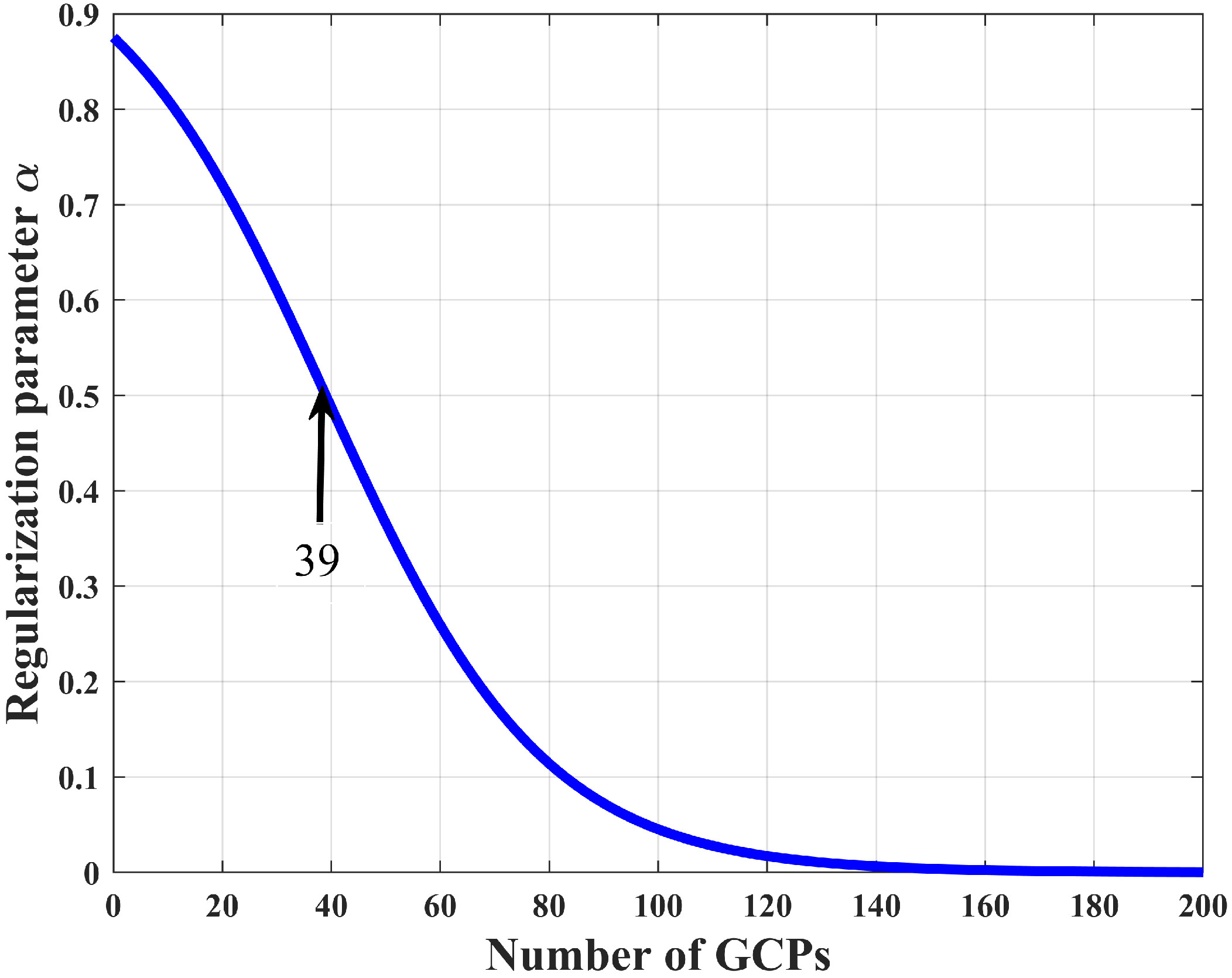
3.2. Adaptive Regularization Parameter Approach

Although there is no need to define a threshold parameter to distinguish signal-related and noise-related PCs, it is still challenging to set the two optimal regularization parameters of the Elastic Net, which significantly affect the sparsity of the eigenvectors. Higher values of $\mu$ and $\alpha$ impose greater penalties on Lasso, resulting in sparser eigenvectors. It is clear that there is a trade-off between sparsity and reconstruction loss. To achieve better performance, we propose an adaptive regularization parameter approach.

When performing Elastic Net regression, the regularization parameter directly determines the sparsity of the eigenvectors. In general, the eigenvalue corresponds to the amount of variance explained by each PC. To obtain more robust eigenvector representations while preserving as much original information as possible, different regularization parameter should be assigned to each eigenvector in the Elastic Net regression process. A smaller eigenvalue indicates the corresponding eigenvector is more related to noise and, thus, a larger regularization penalty should be applied to obtain a sparser representation, reducing the impact of noise and unnecessary variables. Therefore, we assign different regularization parameter to each eigenvector based on the magnitude of its eigenvalue.

Since the SPCA method is implemented through NIPALS, eigenvalues can be obtained through the definition in the following equation.

$$\mathbf{C}{\mathbf{v}}_i={\lambda }_i{\mathbf{v}}_i$$

(19)

The formula representing this adaptive regularization strategy is as follows:

$${\mu }_i={\displaystyle \frac{\tau }{{\lambda }_i}}=\tau {\displaystyle \frac{\left|{\mathbf{v}}_i\right|}{\left|\mathbf{C}{\mathbf{v}}_i\right|}}$$

(20)

where the regularization parameter ${\mu }_i$ is inversely proportional to the eigenvalue ${\lambda }_i$, $\tau$ is a scalar parameter and ${\mathbf{v}}_i$ is the eigenvector for i-th iteration, and $\mathbf{C}$ is the the covariance matrix in Equation (13). Equation (20) enables a dynamically adjusted regularization parameter process.

As shown in Equation (20), we set the regularization parameter to be inversely proportional to the eigenvalue to better utilize the relationship between eigenvalues and regularization parameters. Specifically, eigenvectors with larger eigenvalues capture more data variability, and thus should be assigned a smaller sparsity penalty to retain more original information that is critical for accurate reconstruction. Meanwhile, noise-related eigenvectors with smaller eigenvalues should be assigned larger regularization constraints to eliminate noise-related signals. To this end, we construct a connection between the regularization parameters and the eigenvalues, ensuring a dynamic balance between the preservation of information and the elimination of noise.

Figure 1c also displays the sparsity distribution of the eigenvector in ASPCA-RFM. By comparing Figure 1a,c, through the adaptive regularization parameter approach, the eigenvector is reduced to a zero vector at the 13-th sequence, which is the same as that in PCA-RFM using a preset threshold. Moreover, the sparsity of eigenvectors in Figure 1c shows an increasing trend when employing the adaptive regularization parameter approach, demonstrating the effectiveness of the adaptive algorithm in Equation (20).

When the number of variables (columns) in the design matrix is higher than the number of observed data points (rows), the model’s degrees of freedom are negative, potentially making it unsolvable. Different levels of sparse penalties should be applied according to the degrees of freedom to ensure that there is no significant loss of information when GCPs are sufficient and to reduce the impact of multicollinearity when GCPs are insufficient. Based on this idea, we associate the balance parameter $\alpha$ of $l_1$ and $l_2$ norm with the degrees of freedom.

$$\alpha ={\displaystyle \frac{1}{1+e^{df/20}}}={\displaystyle \frac{1}{1+e^{\left(n-r/2\right)/20}}}$$

(21)

Considering that $\alpha$ must lie within the interval $\left[0,1\right]$, we employed a sigmoid function to normalize the output, ensuring that $\alpha$ remains within this range. In Equation (21), a preset constant value of 20 is used as the divisor of the degrees of freedom, strategically setting 39 GCPs as the center of the sigmoid function, as shown in Figure 2, which is also the boundary point of positive and negative degrees of freedom. This approach effectively prevents $\alpha$ from approaching one under most degrees of freedom, thereby maintaining a balanced regularization effect in different data scenarios. Thus, through normalization by the sigmoid function, $\alpha$ will be larger when degrees of freedom are smaller, applying stronger regularization. Conversely, when the number of GCPs is larger, $\alpha$ will be smaller, reducing the intensity of regularization. This allows dynamic adjustment of the regularization parameter in different data scenarios, maintaining the robustness of the model.

The algorithm returns matrices of modified PCs and eigenvectors. Clearly, the eigenvectors are no longer orthogonal, so the original reconstruction of the design matrix, as shown in Equation (16), is not satisfied in this case. A general way to reconstruct the design matrix is computed by the LS method [21]:

$${\overline{\mathbf{A}}}_{re}={\mathbf{Q}}_k{\left({\mathbf{Q}}_k^T{\mathbf{Q}}_k\right)}^{-1}{\mathbf{Q}}_k^T\overline{\mathbf{A}}$$

(22)

The proof of Equation (22) is shown in Appendix A. Finally, the complete process of the ASPCA-RFM algorithm is provided in Algorithm 2, as follows:

Algorithm 2 $\mathbf{x}=\mathrm{ASPCA}(\mathbf{A},\mathbf{y})$

1: Require: Design Matrix $\mathbf{A}\in {\mathbf{R}}^{2n\times r}$, Observation vector $\mathbf{y}\in {\mathbf{R}}^{2n}$ 2:    $\overline{\mathbf{A}}=\mathbf{A}-mean\left(\mathbf{A}\right)$ 3:    $[{\mathbf{V}}_k,{\mathbf{Q}}_k,k]=\mathrm{NIPALS}\left(\overline{\mathbf{A}}\right)$ 4:    ${\overline{\mathbf{A}}}_{re}={\mathbf{Q}}_k{\left({{\mathbf{Q}}_k}^T{\mathbf{Q}}_k\right)}^{-1}{{\mathbf{Q}}_k}^T\overline{\mathbf{A}}$ 5:    ${\mathbf{A}}_{re}={\overline{\mathbf{A}}}_{re}+mean\left(\mathbf{A}\right)$ 6:    $\mathbf{x}$ is computed by the QR decomposition with column pivoting and LS method for ${\mathbf{A}}_{re}$ 7:    return $\mathbf{x}$

4. Experiments

4.1. Datasets and Metrics

In the experiment, we evaluated our method on six real datasets collected from three different satellite platforms. The detailed information on the datasets is listed in

Table 1. Information about the datasets.

Dataset	Satellite	Area Type	GSD (m)	Coverage (km2)	Elevation Range (m)	No. of GCPs
GF1-A	GF-1	Mountain	16	40 × 40	403∼917	200
GF1-B	GF-1	Urban	16	20 × 20	−22∼280	100
EO1-A	EO-1	Mountain, Lake	30	30 × 30	4907∼5361	250
EO1-B	EO-1	Rural	30	27 × 27	331∼437	120
S2-A	Sentinel-2	Urban, River	60	110 × 110	−55∼1257	80
S2-B	Sentinel-2	Rural	60	110 × 110	847∼1272	300

. All GCPs in these datasets are obtained through an automatic matching algorithm [32] using Landsat-8 satellite images as the geographic reference. In addition, the height information of the GCPs is obtained from the global Digital Elevation Model (DEM) data. Table 1 shows the specific information about each dataset, including the satellite platform, image resolution, elevation range, geographic coverage and the number of matched control points.

GF1-A and GF1-B are two Wide Field View (WFV) images captured from the GF-1 satellite [31], both with a Ground Sampling Distance (GSD) of 16 m. To match the coverage area of the Landsat-8 images, GF1-A and GF1-B are cropped to two sizes: 40 × 40 and 20 × 20 km². The elevation ranges of GF1-A and GF1-B are 403∼917 and −22∼280 m, respectively. The first image was taken in a mountainous area while the second image was captured in an urban area. Using the automatic matching algorithm, 200 and 100 control points were extracted from GF1-A and GF1-B, respectively. Figure 3a,b illustrate the distribution of GCPs in GF1-A and GF1-B, respectively.

In the experiment, we also applied two scenes from the EO-1 satellite [33] with a GSD of 30 m. EO1-A covers a 30 × 30 mountainous area with an elevation range of 4907 to 5361 m, while EO1-B covers a 27 × 27 rural area with an elevation range of 331 to 437 m. Here, 250 and 120 matched GCPs are available for the evaluation of EO1-A and EO1-B, respectively. The distribution of GCPs in EO1-A and EO1-B is shown in Figure 3c,d.

Additionally, the experiment utilized two scenes of remote-sensing images, namely, S2-A and S2-B, captured from the Sentinel-2 satellite [34]. S2-A was collected over an urban area with several distinct rivers, while S2-B was captured over a rural area in the central part of the United States. Both S2-A and S2-B cover an area of 110 × 110 km². The elevation range of S2-A is from −55 to 1257 m, and that of S2-B is from 847 to 1272 m. For testing, 80 and 300 evenly distributed control points were extracted for S2-A and S2-B, respectively. The distribution of GCPs in S2-A and S2-B is shown in Figure 3e,f.

To better examine the impact of the varying number and distribution of GCPs on the results, we referred to the approach in APCA-RFM [6]. The GCPs in each dataset were divided into two parts by random sampling. The first part randomly selected a fixed number of GCPs from the dataset for the estimation of RPCs, while the second part consisted of the remaining GCPs that were used as Independent Check Points (ICPs) for the accuracy evaluation. For each dataset, this random sampling operation was repeated five times to obtain five Root Mean Square Error (RMSE) metrics, and their average and standard deviation are used as final evaluation metrics. Thus, the average RMSEs can reflect the accuracy of the performance, and the standard deviation values can reflect the stability under different distributions of GCPs. For example, GF1-A has 200 available control points. To verify the performance of the algorithm with 40 GCPs, five times random sampling operations were conducted, each with 40 points as GCPs and the remaining 160 points as ICPs, to calculate the RMSE metrics. The RMSE metric can be computed by the following formula [35]:

$$RMSE=\sqrt{{\displaystyle \frac{1}{N}}\sum _{i=1}^N({\epsilon }_{li}^2+{\epsilon }_{si}^2)}$$

(23)

where ${\epsilon }_l$ and ${\epsilon }_s$ denote the line and sample error, respectively. N represents the number of ICPs.

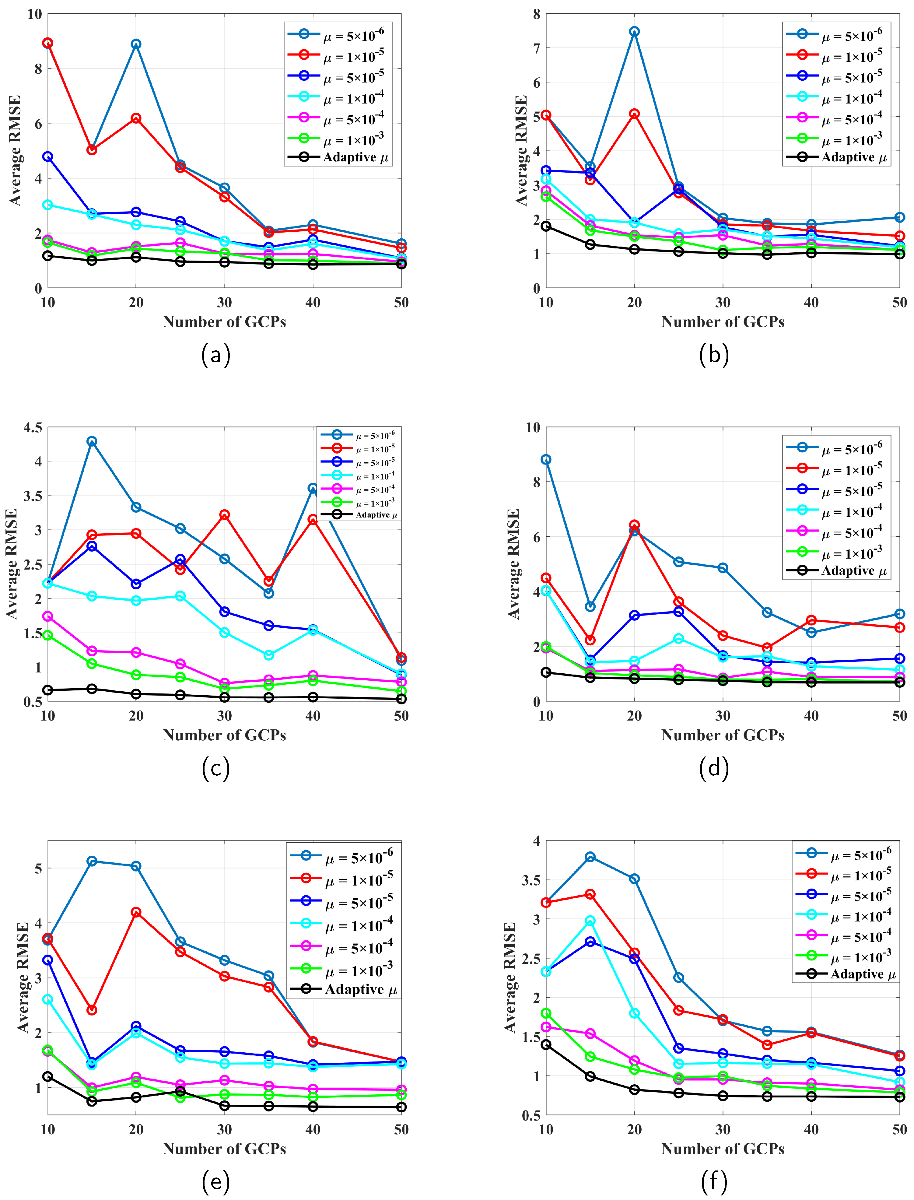
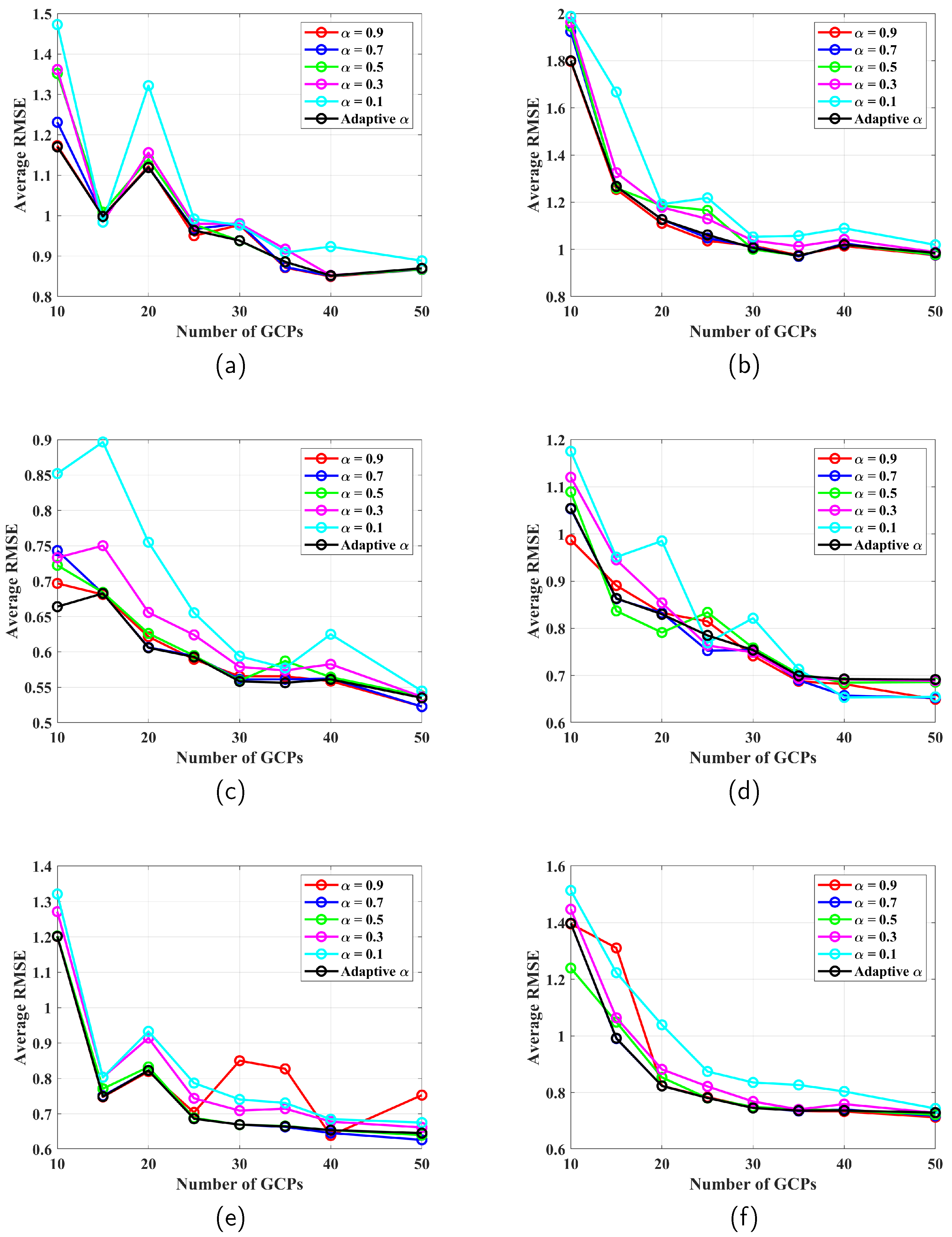
4.2. Parameter Setting of the Methods in Comparison

In this study, to verify the effectiveness of the proposed method, four state-of-the-art methods, namely ridge estimation [7], L1LS [9], PCA-RFM [20] and APCA-RFM [6], were applied to various datasets for comparison. The L1LS method provided stable and sparse RPC results using L1-norm-regularized least squares when the available observation data were relatively insufficient. The APCA-RFM method separated the noise-related PCs from the signal-related ones by using an automatic thresholding ridge ratio. For the ridge estimation method, the parameter $\lambda$ was manually set to ${10}^{-4}$. In the L1LS method, previous analysis in [9] has shown that $\lambda ={10}^{-4}$ is the optimal choice. The PCA-RFM method set the threshold parameter t to 0.01. In the proposed method, the scalar value $\tau$ was set to 8 × ${10}^{-5}$, and the Elastic Net was solved using the coordinate descent algorithm [36]. All experiments were conducted and tested on a 13-th Gen Intel Core i5 CPU at 2.50 GHz and 15.70 GB usable RAM.

4.3. Comparative Results

In this experiment, the analysis is divided into two main parts: analysis with a sufficient number of GCPs (positive degrees of freedom) and analysis with a limited number of GCPs (negative degrees of freedom). In the first part, 40 and 50 GCPs were selected to compute RPCs using different experimental algorithms while the remaining GCPs were used as evaluation sets. In the second part, the performance of different methods was investigated on datasets with only 10, 15 and 20 GCPs, respectively. The results of the quantitative evaluation in terms of the average and standard deviation of RMSE on the six datasets and the different numbers of GCPs are shown in

Table 2. Average and standard deviation values (in pixels) for different methods evaluated on datasets.

Dataset	GCPs/ICPs	Ridge Estimation	L1LS	PCA-RFM	APCA-RFM	ASPCA-RFM
GF1-A	10/190	286.52 ± 115.44	3.8254 ± 2.5172	2.6414 ± 3.0570	2.5632 ± 3.0873	1.1704 ± 0.1413
	15/185	69.087 ± 23.892	1.7546 ± 0.6008	1.0119 ± 0.1279	1.0017 ± 0.1106	0.9980 ± 0.0958
	20/180	48.835 ± 37.972	1.7815 ± 0.3979	1.1274 ± 0.2124	1.2313 ± 0.3530	1.1193 ± 0.2361
	40/160	4.4347 ± 1.6321	1.5912 ± 0.3304	0.8598 ± 0.0322	0.8382 ± 0.0289	0.8519 ± 0.0265
	50/150	3.0036 ± 1.4762	1.3455 ± 0.1606	0.8629 ± 0.0430	0.8489 ± 0.0394	0.8699 ± 0.0387
GF1-B	10/90	83.932 ± 21.314	3.1493 ± 4.2251	1.9714 ± 0.4728	1.8910 ± 0.6624	1.7997 ± 0.5219
	15/85	44.755 ± 22.098	4.2002 ± 4.2721	1.3033 ± 0.2391	1.5418 ± 0.6608	1.2666 ± 0.2015
	20/80	12.587 ± 5.5499	1.2065 ± 0.2709	1.1808 ± 0.0900	1.1688 ± 0.1349	1.1266 ± 0.0586
	40/60	7.8813 ± 8.3771	3.0036 ± 3.9359	1.0754 ± 0.1423	0.9914 ± 0.0511	1.0201 ± 0.0472
	50/50	7.3447 ± 10.400	3.3032 ± 4.2816	0.9870 ± 0.0583	0.9836 ± 0.0730	0.9850 ± 0.0578
EO1-A	10/240	109.31 ± 33.435	1.5254 ± 1.0866	0.7464 ± 0.1207	0.7741 ± 0.1235	0.6639 ± 0.0747
	15/235	58.242 ± 24.074	0.8955 ± 0.2221	0.6998 ± 0.1110	0.6995 ± 0.1325	0.6827 ± 0.0991
	20/230	24.292 ± 12.448	0.8026 ± 0.1566	0.6768 ± 0.0831	0.6152 ± 0.0834	0.6059 ± 0.0261
	40/210	4.0333 ± 1.7325	0.7326 ± 0.0876	0.5615 ± 0.0314	0.5622 ± 0.0664	0.5612 ± 0.0403
	50/200	1.4546 ± 0.5880	0.6847 ± 0.0407	0.5384 ± 0.0342	0.5172 ± 0.0163	0.5351 ± 0.0396
EO1-B	10/110	145.15 ± 51.848	3.6538 ± 4.1398	1.1291 ± 0.3580	1.2531 ± 0.9818	1.0544 ± 0.3865
	15/105	44.734 ± 14.071	1.3268 ± 0.2681	0.9563 ± 0.1560	0.9571 ± 0.2341	0.8635 ± 0.0599
	20/100	27.488 ± 10.997	1.1318 ± 0.3017	0.8690 ± 0.1708	0.8970 ± 0.1278	0.8299 ± 0.0847
	40/80	4.4904 ± 3.5525	0.9986 ± 0.1542	0.6987 ± 0.1015	0.7515 ± 0.1123	0.6927 ± 0.0565
	50/70	2.2041 ± 0.6681	0.9495 ± 0.1838	0.6770 ± 0.0823	0.6518 ± 0.0542	0.6915 ± 0.1411
S2-A	10/70	168.88 ± 74.618	6.0041 ± 2.7493	1.2099 ± 0.4341	1.4811 ± 0.4198	1.2015 ± 0.4081
	15/65	107.80 ± 93.904	4.6899 ± 3.2891	0.7706 ± 0.1451	0.8446 ± 0.2767	0.7485 ± 0.1598
	20/60	107.84 ± 106.98	4.8182 ± 3.7693	0.8929 ± 0.3100	1.0044 ± 0.2442	0.8224 ± 0.2362
	40/40	36.784 ± 34.181	2.0378 ± 0.7463	0.6694 ± 0.0356	0.7820 ± 0.2396	0.6538 ± 0.0277
	50/30	20.586 ± 21.144	1.5930 ± 0.8513	0.6606 ± 0.0694	0.8995 ± 0.3331	0.6452 ± 0.0418
S2-B	10/290	107.13 ± 32.422	2.1641 ± 0.5022	1.2462 ± 0.3278	1.3315 ± 0.5066	1.3981 ± 0.5374
	15/285	59.161 ± 31.510	2.1688 ± 0.5086	1.0541 ± 0.3425	1.5211 ± 0.7938	0.9921 ± 0.3166
	20/280	22.722 ± 18.665	1.6835 ± 0.3464	0.9005 ± 0.1483	0.9135 ± 0.2239	0.8233 ± 0.0686
	40/260	2.9398 ± 1.5114	1.7074 ± 0.3256	0.7457 ± 0.0193	1.0462 ± 0.7065	0.7366 ± 0.0065
	50/250	1.9344 ± 0.5927	1.6297 ± 0.1987	0.7217 ± 0.0103	0.7177 ± 0.0082	0.7290 ± 0.0252

, where the best results for each experiment are highlighted in bold. The average value directly indicates the error magnitude of the method, while the variance reflects the robustness of the method to different distributions of GCPs.

As shown in Table 2, although the ridge estimation method has the weakest performance among the tested methods, it yields reasonable results when there is an adequate number of GCPs. In contrast, when the number of GCPs is limited, the L1LS method produces relatively stable results, but its performance is still inferior to the PCA-based RFM methods. With an adequate number of GCPs, the proposed ASPCA-RFM method shows comparable performance to the APCA-RFM method across all datasets. For the GF1-A and GF1-B datasets, the APCA-RFM method performs the best in terms of average RMSE, while the ASPCA-RFM method performs the best in terms of standard deviation (with 40 and 50 GCPs). In particular for the S2-A dataset, the proposed method shows higher precision than other methods in both the average and standard RMSEs. For 40 and 50 GCPs, except for GF1-B, the average RMSEs of the proposed method are below one pixel across all datasets. When the degrees of freedom are positive, the results of the ASPCA-RFM and APCA-RFM methods are close, with ASPCA-RFM sometimes slightly inferior to APCA-RFM.

When the number of GCPs is far less than 39, the RPC estimation problem is severely affected by ill-posedness and overparameterization. The ridge estimation method performs poorly and almost fails when using 20, 15 and 10 GCPs whereas the L1LS method improves the solution of ridge estimation and shows strong robustness. Even in the 10-GCP case, PCA-based methods can provide practically feasible results. With a limited number of GCPs, the proposed method shows better performance by a marked margin on almost all datasets and for all numbers of GCPs. In particular, on the GF1-A dataset, the proposed ASPCA-RFM method further reduces the average RMSE pixel value by 1.4 compared to the second-best model when using 10 GCPs. Besides the average RMSE metric, the proposed method also achieves higher RMSE standard deviation values on almost all datasets, indicating better robustness under different GCP distributions. The analysis in the table shows that, with a limited number of GCPs, the ASPCA-RFM method outperforms other methods in both average RMSE and standard deviation of RMSE.

In the experiment, we also compared the average computational time of the proposed method and the other methods, as shown in

Table 3. Average computational time for different methods on all datesets. ASPCA-RFM-EVD is our proposed method implemented based on EVD.

Ridge Estimation	L1LS	PCA-RFM	APCA-RFM	ASPCA-RFM-EVD	ASPCA-RFM (Ours)
0.0008 s	0.0013 s	0.0009 s	0.0021 s	0.0845 s	0.0454 s

. The computational cost of ASPCA-RFM is higher than the other methods as it requires multiple Elastic Net regression operations. However, all methods are fast and require less than 0.1 s per run, which is sufficient to support practical applications. To verify the efficiency of our proposed method optimized by NIPALS, we also implemented the ASPCA-RFM based on EVD, namely ASPCA-RFM-EVD. In Table 3, our proposed method is much faster than ASPCA-RFM-EVD, which demonstrates the effectiveness of NIPALS. On the other hand, in general, EVD is more reliable in terms of numerical stability compared to NIPALS. The setting of the initial value, iteration stopping criteria and number of iterations in NIPALS may affect the quality of the final results. However, according to the setting in Algorithm 1, we can ensure that the results optimized by EVD and NIPALS are the same to the third decimal place, which indicates that both optimization methods yield almost the same numerical quality.

4.4. Model Analysis

The adaptive regularization parameter approach aims to dynamically assign suitable regularization parameters for different PCs and different numbers of observation data. To investigate its effect, we conducted an experiment to understand the behavior of the adaptive regularization parameter approach in ASPCA-RFM. We randomly selected different numbers of GCPs from six datasets, specifically 50, 40, 30, 20 and 10. In the experiment, the number of zero values for each eigenvector was counted and summarized, representing the sparsity for each vector. Figure 4 illustrates the variation in sparsity with eigenvectors across all datasets and the overall trend under different numbers of GCPs. The eigenvectors are sorted in descending order of eigenvalues. From the perspective of different eigenvectors, in all results, the sparsity gradually increases with the order of the eigenvectors, indicating that eigenvectors with smaller eigenvalues correspond to higher sparsity. The results show that the adaptive regularization parameter strategy we described in Equation (20) was accurately executed. From the perspective of different numbers of GCPs, overall, as the number of GCPs increases, sparsity shows a decreasing trend. This validates the mathematical design of the adaptive regularization parameter, as shown in Equation (21), making the ASPCA-RFM algorithm more robust when faced with insufficient and unevenly distributed GCPs.

To better understand the efficiency of the adaptive regularization parameter approach, we designed two comparative experiments to demonstrate the performance advantages of the adaptive regularization parameter algorithm over fixed regularization parameters. In the first comparative experiment, the adaptive overall penalty coefficient $\mu$ in Equation (20) was replaced with fixed values, specifically 5 × ${10}^{-6}$, 1 × ${10}^{-5}$, 5 × ${10}^{-5}$, 1 × ${10}^{-4}$, 5 × ${10}^{-4}$ and 1 × ${10}^{-3}$. The performance of different fixed values and the adaptive regularization parameter approach was tested under different numbers of GCPs on six datasets, and the average RMSE results are shown in Figure 5. The results showed that, as $\mathsf{\mu }$ changed, the error fluctuated significantly, but the adaptive algorithm consistently maintained the lowest RMSE values. It is clear that, in nearly all datasets and GCPs, the method using the adaptive regularization parameter achieved the best performance, fully demonstrating the effectiveness of adaptive regularization parameters.

The second comparative experiment aims to compare the performance difference between the adaptive strategy and fixed values for the balance regularization parameter $\alpha$. Similar to the first comparative experiment, the adaptive $\alpha$ in Equation (21) was replaced with fixed values, specifically 0.9, 0.7, 0.5, 0.3 and 0.1. The experimental results for different numbers of GCPs in six datasets are shown in Figure 6, with all the results presented using the average RMSE. From an overall perspective, the adaptive regularization parameters outperform the fixed values in most scenarios. On the other hand, compared to the adaptive algorithm, fixed regularization parameters may perform better for specific numbers of GCPs or specific datasets, but their stability is much lower. Most importantly, there is no single fixed value that performs best across all GCPs and datasets. For example, in the GF1-A dataset of Figure 6a, when $\alpha =0.1$, although this fixed parameter achieves the best result when the number of GCPs is 15, it results in very high RMSE values for the other numbers of GCPs. In the EO1-B dataset of Figure 6d, although the results for $\alpha =0.5$ were the best when the GCPs were 15 and 20, the RMSE was the worst when the GCPs were 25, and the performance for other numbers of GCPs was also inferior to the adaptive algorithm. In summary, although the adaptive balance regularization parameter did not achieve the best results in all datasets and all numbers of GCPs, compared to the fixed values, the adaptive algorithm consistently achieved stable and lower RMSE values. This demonstrated its effectiveness in adaptively adjusting the regularization parameters based on the number of GCPs, ultimately achieving more robust results.

5. Conclusions

In this paper, an adaptive Sparse Principal Component Analysis method is proposed for RPC estimation to address the problems of ill-posedness and overparameterization. The ASPCA-RFM introduces the SPCA to obtain sparse eigenvectors, which reduces the impact of noise and errors in the design matrix. Considering the high computational cost of performing Elastic Net regression on each PC, we propose using the NIPALS framework to perform Elastic Net regression only on signal-related eigenvectors and automatically remove unnecessary PCs. To further improve performance, we propose an adaptive regularization parameter approach that can dynamically adjust the regularization parameters based on the explained variance of PCs and the amount of observation data.

Extensive experiments have been conducted and the results show that the proposed ASPCA-RFM outperforms or is highly competitive with existing RFM models. In particular, the proposed method performs better than other methods when the number of GCPs is limited. The experimental results demonstrate that the proposed adaptive regularization parameter approach can achieve a great balance between sparsity and information loss. In future work, we will investigate a more reliable method for dynamically changing the regularization parameters, especially in cases with a sufficient number of GCPs. In addition, considering that deep learning methods have demonstrated significant performance improvements compare with traditional methods, we plan to explore a deep learning-based RPC estimation method in our future work. The proposed RPC estimation method may contribute to the practical application of optical satellites.

References

1. Shen, X.; Li, Q.; Wu, G.; Zhu, J. Bias compensation for rational polynomial coefficients of high-resolution satellite imagery by local polynomial modeling. Remote Sens. 2017, 9, 200. [Google Scholar] [CrossRef]
2. Toutin, T. Geometric processing of remote sensing images: Models, algorithms and methods. Int. J. Remote Sens. 2004, 25, 1893–1924. [Google Scholar] [CrossRef]
3. Zhang, L.; He, X.; Balz, T.; Wei, X.; Liao, M. Rational function modeling for spaceborne SAR datasets. ISPRS J. Photogramm. Remote Sens. 2011, 66, 133–145. [Google Scholar] [CrossRef]
4. Zhou, G.; Liu, X. Orthorectification model for extra-length linear array imagery. IEEE Trans. Geosci. Remote Sens. 2022, 60, 1–10. [Google Scholar] [CrossRef]
5. Tao, C.V.; Hu, Y. A comprehensive study of the rational function model for photogrammetric processing. Photogramm. Eng. Remote Sens. 2001, 67, 1347–1358. [Google Scholar]
6. Gholinejad, S.; Amiri-Simkooei, A.; Moghaddam, S.H.A.; Naeini, A.A. An automated PCA-based approach towards optimization of the rational function model. ISPRS J. Photogramm. Remote Sens. 2020, 165, 133–139. [Google Scholar] [CrossRef]
7. Yuan, X.; Lin, X. A method for solving rational polynomial coefficients based on ridge estimation. Geomat. Inf. Sci. Wuhan Univ. 2008, 33, 1130–1133. [Google Scholar]
8. Wu, Y.; Ming, Y. A fast and robust method of calculating RFM parameters for satellite imagery. Remote Sens. Lett. 2016, 7, 1112–1120. [Google Scholar] [CrossRef]
9. Long, T.; Jiao, W.; He, G. Rpc estimation via L1-norm-regularized least squares (l1ls). IEEE Trans. Geosci. Remote Sens. 2015, 53, 4554–4567. [Google Scholar] [CrossRef]
10. Gholinejad, S.; Naeini, A.A.; Amiri-Simkooei, A. Optimization of RFM Problem Using Linearly Programed l1-Regularization. IEEE Trans. Geosci. Remote Sens. 2021, 60, 1–9. [Google Scholar] [CrossRef]
11. Zhao, L.; Liu, F.; Li, J.; Wang, W. Research on reducing term of higher order in RFM model. Sci. Surv. Mapp. 2007, 32, 14–17. [Google Scholar]
12. Zhang, Y.; Lu, Y.; Wang, L.; Huang, X. A new approach on optimization of the rational function model of high-resolution satellite imagery. IEEE Trans. Geosci. Remote Sens. 2011, 50, 2758–2764. [Google Scholar] [CrossRef]
13. Moghaddam, S.H.A.; Mokhtarzade, M.; Moghaddam, S.A.A. Optimization of RFM’s structure based on PSO algorithm and figure condition analysis. IEEE Geosci. Remote Sens. Lett. 2018, 15, 1179–1183. [Google Scholar] [CrossRef]
14. Tengfei, L.; Weili, J.; Guojin, H. Nested regression based optimal selection (NRBOS) of rational polynomial coefficients. Photogramm. Eng. Remote Sens. 2014, 80, 261–269. [Google Scholar] [CrossRef]
15. Moghaddam, S.H.A.; Mokhtarzade, M.; Naeini, A.A.; Amiri-Simkooei, A. A statistical variable selection solution for RFM ill-posedness and overparameterization problems. IEEE Trans. Geosci. Remote Sens. 2018, 56, 3990–4001. [Google Scholar]
16. Zoej, M.V.; Mokhtarzade, M.; Mansourian, A.; Ebadi, H.; Sadeghian, S. Rational function optimization using genetic algorithms. Int. J. Appl. Earth Obs. Geoinf. 2007, 9, 403–413. [Google Scholar]
17. Zhou, G. On-Board Processing for Satellite Remote Sensing Images; CRC Press: Boca Raton, FL, USA, 2023. [Google Scholar]
18. Cavallaro, G.; Heras, D.B.; Wu, Z.; Maskey, M.; Lopez, S.; Gawron, P.; Coca, M.; Datcu, M. High-Performance and Disruptive Computing in Remote Sensing: HDCRS—A new Working Group of the GRSS Earth Science Informatics Technical Committee [Technical Committees]. IEEE Geosci. Remote Sens. Mag. 2022, 10, 329–345. [Google Scholar] [CrossRef]
19. Zhang, R.; Zhou, G.; Zhang, G.; Zhou, X.; Huang, J. RPC-based orthorectification for satellite images using FPGA. Sensors 2018, 18, 2511. [Google Scholar] [CrossRef]
20. Naeini, A.A.; Moghaddam, S.H.A.; Sheikholeslami, M.M.; Amiri-Simkooei, A. Application of PCA Analysis and QR Decomposition to Address RFM’s Ill-Posedness. Photogramm. Eng. Remote Sens. 2020, 86, 17–21. [Google Scholar] [CrossRef]
21. Golub, G.H.; Van Loan, C.F. Matrix Computations; JHU Press: Baltimore, MD, USA, 2013. [Google Scholar]
22. Hao, L.; Pan, C.; Liu, P.; Zhou, D.; Zhang, L.; Xiong, Z.; Liu, Y.; Sun, G. Detection of the coupling between vegetation leaf area and climate in a multifunctional watershed, Northwestern China. Remote Sens. 2016, 8, 1032. [Google Scholar] [CrossRef]
23. Li, J.; Fan, K.; Zhou, L. Satellite observations of El Niño impacts on Eurasian spring vegetation greenness during the period 1982–2015. Remote Sens. 2017, 9, 628. [Google Scholar] [CrossRef]
24. Zou, H.; Hastie, T.; Tibshirani, R. Sparse principal component analysis. J. Comput. Graph. Stat. 2006, 15, 265–286. [Google Scholar] [CrossRef]
25. Zou, H.; Hastie, T. Regularization and variable selection via the elastic net. J. R. Stat. Soc. Ser. B Stat. Methodol. 2005, 67, 301–320. [Google Scholar] [CrossRef]
26. Wold, H.O.A. Nonlinear Estimation by Iterative Least Square Procedures. In Research Papers in Statistics: Festschrift for J. Neyman; David, F.N., Ed.; Wiley: New York, NY, USA, 1966. [Google Scholar]
27. Zhou, G.; Yuan, M.; Li, X.; Sha, H.; Xu, J.; Song, B.; Wang, F. Optimal regularization method based on the L-curve for solving rational function model parameters. Photogramm. Eng. Remote Sens. 2021, 87, 661–668. [Google Scholar] [CrossRef]
28. Tibshirani, R. Regression shrinkage and selection via the lasso. J. R. Stat. Soc. Ser. B Stat. Methodol. 1996, 58, 267–288. [Google Scholar] [CrossRef]
29. Kincaid, D.R.; Cheney, E.W. Numerical Analysis: Mathematics of Scientific Computing; American Mathematical Society: Providence, RI, USA, 2009; Volume 2. [Google Scholar]
30. Hotelling, H. Analysis of a complex of statistical variables into principal components. J. Educ. Psychol. 1933, 24, 417. [Google Scholar] [CrossRef]
31. Zhang, G.; Xu, K.; Huang, W. Auto-calibration of GF-1 WFV images using flat terrain. ISPRS J. Photogramm. Remote Sens. 2017, 134, 59–69. [Google Scholar] [CrossRef]
32. Fan, Z.; Liu, Y.; Liu, Y.; Zhang, L.; Zhang, J.; Sun, Y.; Ai, H. 3MRS: An effective coarse-to-fine matching method for multimodal remote sensing imagery. Remote Sens. 2022, 14, 478. [Google Scholar] [CrossRef]
33. Ungar, S.G.; Pearlman, J.S.; Mendenhall, J.A.; Reuter, D. Overview of the earth observing one (EO-1) mission. IEEE Trans. Geosci. Remote Sens. 2003, 41, 1149–1159. [Google Scholar] [CrossRef]
34. Drusch, M.; Del Bello, U.; Carlier, S.; Colin, O.; Fernandez, V.; Gascon, F.; Hoersch, B.; Isola, C.; Laberinti, P.; Martimort, P.; et al. Sentinel-2: ESA’s optical high-resolution mission for GMES operational services. Remote Sens. Environ. 2012, 120, 25–36. [Google Scholar] [CrossRef]
35. Shan, X.; Zhang, J. Does the Rational Function Model’s Accuracy for GF1 and GF6 WFV Images Satisfy Practical Requirements? Remote Sens. 2023, 15, 2820. [Google Scholar] [CrossRef]
36. Friedman, J.; Hastie, T.; Tibshirani, R. Regularization paths for generalized linear models via coordinate descent. J. Stat. Softw. 2010, 33, 1. [Google Scholar] [CrossRef] [PubMed]
Figure 1. Distribution of sparsity for eigenvectors tested on GF1−A dataset with 20 GCPs. (a) Sparsity of eigenvectors using PCA. (b) Sparsity of eigenvectors using SPCA with fixed regularization parameters. (c) Sparsity of eigenvectors using ASPCA−RFM with adaptive regularization parameters.
Remotesensing 16 03018 g001
Figure 2. Sigmoid form of the regularization parameter α . Thirty-nine GCPs are the center point of the sigmoid function which is also the boundary point of positive and negative degrees of freedom.
Remotesensing 16 03018 g002
Figure 3. Distribution of GCPs for different datasets. (a) GF1-A. (b) GF1-B. (c) EO1-A. (d) EO1-B. (e) S2-A. (f) S2-B.
Remotesensing 16 03018 g003
Figure 4. Sparsity of different eigenvectors when handling different numbers of GCPs on six datasets. (a) GF1-A. (b) GF1-B. (c) EO1-A. (d) EO1-B. (e) S2-A. (f) S2-B.
Remotesensing 16 03018 g004
Figure 5. Average RMSE results for fixed μ and adaptive μ . (a) GF1-A. (b) GF1-B. (c) EO1-A. (d) EO1-B. (e) S2-A. (f) S2-B.
Remotesensing 16 03018 g005
Figure 6. Average RMSE results for fixed α and adaptive α . (a) GF1-A. (b) GF1-B. (c) EO1-A. (d) EO1-B. (e) S2-A. (f) S2-B.
Remotesensing 16 03018 g006