Field Measurements of Spatial Air Emissions from Dairy Pastures Using an Unmanned Aircraft System

Abstract

Unmanned aircraft systems (UASs) are emerging as useful tools in environmental studies due to their mobility and ability to cover large areas. In this study, we used an air analyzer attached to a UAS to measure gas and particulate matter (PM) emissions from rotationally grazed dairy pastures in northern Wisconsin. UAS-based sampling enabled wireless data transmission using the LoRa protocol to a ground station, synchronizing with a cloud server. During the measurements, latitude, longitude, and altitude were recorded using a high-precision global positioning system (GPS). Over 1200 measurements per parameter were made during each site visit. The spatial distribution of the emission rates was estimated using the Lagrangian mass balance approach and Kriging interpolation. A horizontal sampling probe effectively minimized the impact of propeller downwash on the measurements. The average concentrations of carbon dioxide (CO₂), methane (CH₄), and nitrous oxide (N₂O) were 800.1 ± 39.7 mg m⁻³, 1.38 ± 0.063 mg m⁻³, and 0.71 ± 0.03 mg m⁻³, respectively. No significant difference was found between CO₂ concentrations measured by the UAS sensor and gas chromatography (p = 0.061). Emission maps highlighted variability across the pasture, with an average CO₂ emission rate of 1.52 ± 0.80 g day⁻¹ m⁻², which was within the range reported in the literature. Future studies could explore the impact of pasture management on air emissions.

1. Introduction

Unmanned aircraft systems (UASs) weighing less than 24.9 kg (55 lbs) are defined by the United States Federal Aviation Administration as small unmanned aircraft systems (sUAS) [1,2]. These aircraft systems are gaining increased recognition in research across a broad spectrum of applications [2,3]. For example, UASs are now being proposed for environmental monitoring to measure air emissions [2,3,4]. Standard air sampling methods rely on fixed, stationary air quality monitoring systems. While these systems are reliable, they are limited by their immobility and restricted spatial coverage [5]. The mobility of UASs and their ability to cover large areas make them advantageous when traditional measurement techniques cannot be used due to the scale of the area being monitored [2].

Although UASs have advantages, there are two main challenges regarding UAS-based air sampling: (i) sensors need to be lightweight to be carried by a UAS, and (ii) the impact of propeller downwash has to be accounted for during measurements. To mitigate the impact of downwash on sampling, a few existing commercial systems (e.g., Aeromon BH-12, Turku, Finland; Scentroid DR2000, Stouffville, Ontario, Canada; and FLIR Muve C360, Arlington, VA, USA) have suggested utilizing a horizontal sampling probe in order to collect samples outside the rotor’s influence. This method was found to be effective when the UAS operates close to the ground, enabling it to capture emissions directly from the surface [6,7,8].

In recent years, UAS-based air sampling has been extended to mapping gas concentrations, which involves generating spatial maps that represent gas concentrations within a specific region. This is achieved by utilizing a collection of sensor measurements distributed across the area. While this type of map can be used to evaluate the dispersion of gasses within an area, it can also be utilized to pinpoint the location of gas sources and calculate fluxes [9]. Previous studies employed UAS-based sampling for mapping concentrations of air pollutants in both indoor and outdoor areas, as well as in larger controlled environments such as livestock facilities, greenhouses, and landfills [10,11,12].

Building on this approach, UAS-based sampling can also be used to map air emission rates. Two methods to estimate emission rates include the mass balance method [2,13] and the Gaussian dispersion approach [14,15]. The mass balance method combined with Kriging interpolation was reported to be suitable for UAS-based measurements [2,16]. In a recent study, a UAS was used to quantify CH₄ emissions from dairy buildings, and it was found that the UAS-based mass balance approach combined with Kriging interpolation can accurately quantify CH₄ emissions from these facilities [2]. In another study, a mass balance flux method was developed to measure CH₄ emissions from landfills using a UAS. It was concluded that this method could be used to prepare source-specific greenhouse gas emission inventories [16].

Although there has been a growing interest in quantifying air emissions, particularly greenhouse gas emissions from dairy facilities [17,18,19], research has shown varying results for the emission rates. Some studies suggest that confinement systems emit less greenhouse gasses per pound of milk or meat produced compared to pastures [20]. It was also reported that grass-based livestock farms had the lowest net greenhouse gas emissions [20]. Considering that the data in the literature mostly rely on modeling approaches [21], there is a need for research that focuses on direct measurements to enhance our understanding of air emissions from livestock facilities.

In contrast to previous studies that used static [22] or dynamic flux chambers [23], which sampled only a partial surface of the pasture, in this study, we surveyed the entire surface area of the pasture using our UAS-based air sampling system. Surveying the entire surface and generating a spatial distribution is important because emission rates vary significantly with different sampling locations [23]. The objectives of this study are (i) to measure CO₂, ammonia (NH₃), nitrogen dioxide (NO₂), hydrogen sulfide (H₂S), total volatile organic compounds (TVOCs), and particulate matter (PM₁, PM_2.5, and PM₁₀) concentrations using a UAS-based sampling system; (ii) to verify the applicability of collecting air samples in air sampling bags during the flights to be analyzed in the laboratory using gas chromatography (GC) coupled with a flame ionization detector (FID: CO₂, CH₄) and an electron capture detector (ECD: N₂O); and (iii) to calculate air emissions and estimate the spatial distribution over the pasture using the Lagrangian mass balance approach and Kriging interpolation.

2. Materials and Methods

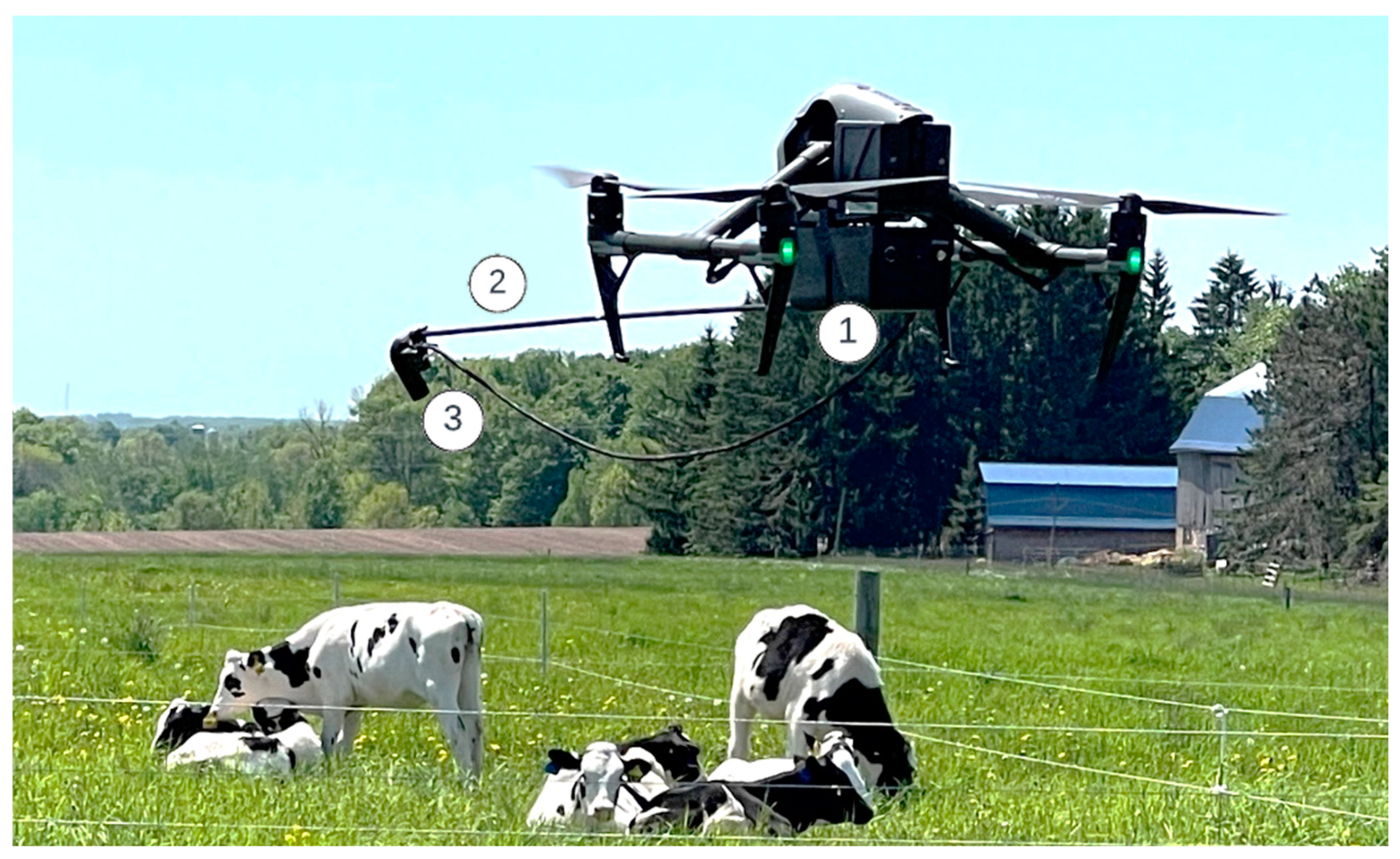
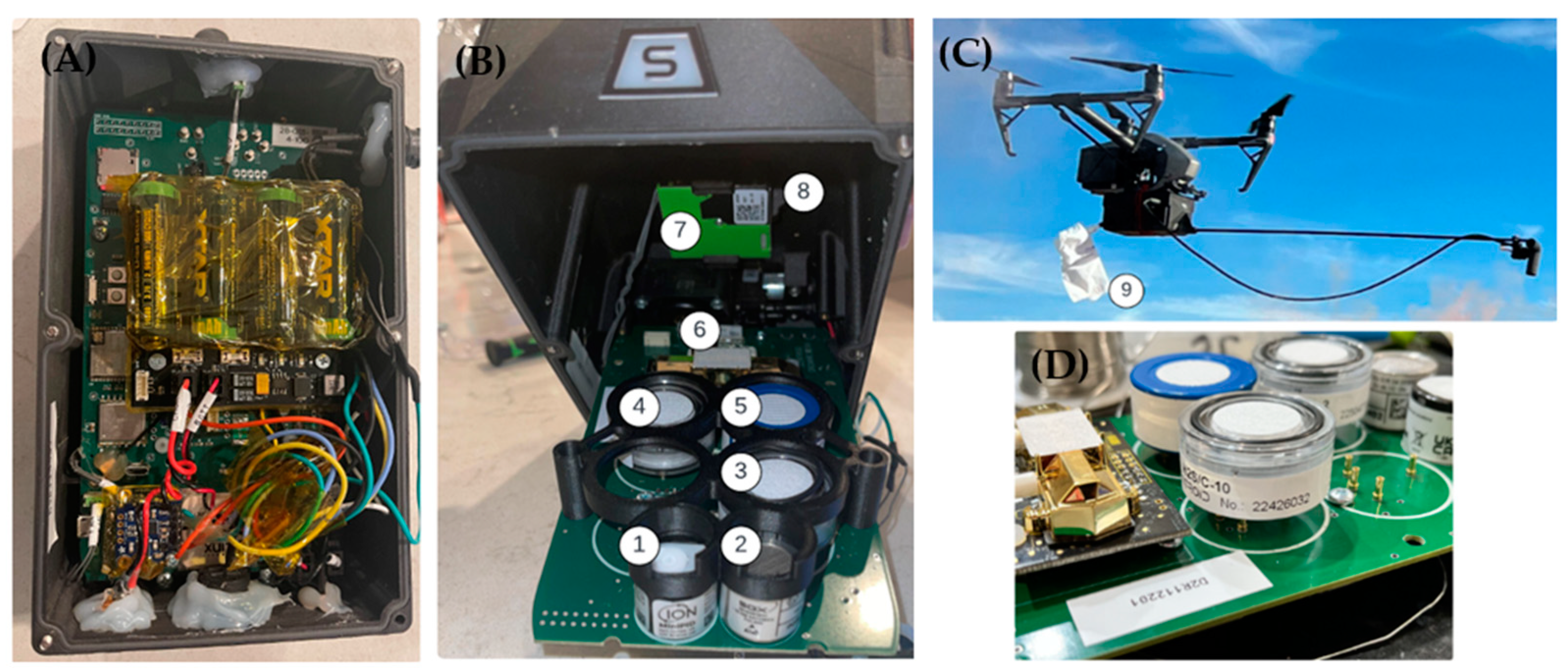
2.1. Unmanned Aircraft System and Air Analyzer

A UAS (DJI Inspire II, Shenzhen, Guangdong, China), with a maximum takeoff weight capacity of 4250 g, was used in this study. Both the first and corresponding authors of this manuscript had a remote pilot license issued by the U.S. Federal Aviation Administration to operate this UAS. An 800 g (23 × 10.8 × 10.3 cm) air analyzer (DR2000, Scentroid, Stouffville, ON, Canada) was attached to the UAS. Figure 1 and Figure 2 show the UAS and air analyzer parts, respectively. The air analyzer was equipped with CO₂, CH₄, NH₃, NO_x, H₂S, TVOCs, PM₁, PM_2.5, and PM₁₀ sensors.

Table 1. DR2000 sensors, ranges, and resolutions ¹.

Parameter	Sensor Type	Range
CO2	NDIR	1 to 2000 ppm
NH3	EC	0.005 ppm to 10 ppm
NOx	EC	0.01 to 1 ppm
H2S	EC	7 ppb to 3 ppm
CH4	NDIR	0.4 to 100 ppm
Total VOCs	PID	1 ppb to 50 ppm
PM1, PM2.5, PM10	Laser-scattered	1 to 2000 µg m−3
Temperature	-	5 to 40 °C
Humidity	-	10 to 90%
Barometric pressure	-	-
Inertial movement unit	Wind direction, compass	-
Wind speed	-	0.3 to 67 m s−1

¹ NDIR: nondispersive infrared sensor; EC: electrochemical sensor; PID: photo-ionization sensor.

shows the sensor types and detection thresholds. Additionally, the air analyzer included temperature, humidity, barometric pressure, wind speed, and wind direction sensors, a compass for true North location, and a high-precision global positioning system (GPS) for latitude/longitude and altitude measurements. All sensors were calibrated and certified annually. The particulate matter sensor calibration was performed according to the ISO 21501-4 standard [24]. An example of calibration data is shown in Table S1. The system enabled wireless data transmission using the LoRa protocol for secure encrypted transmission to the ground station. The ground station, equipped with DRIMS-GS software version 3.2., enabled the live monitoring of all parameters and auto Sync with DRIMS2 cloud software (version 4.1., Scentroid, Stouffville, ON, Canada).

The air analyzer had two key features. One was an 88 cm long horizontal sampling probe, which enabled the collection of air samples outside of the propeller downwash. The effectiveness of this sampling probe was tested using a smoke test, with the probe oriented upwind (discussed in Section 3.1). The other feature was a sample acquisition system, which allowed for remote grab sampling during flights, capturing samples in customized 1 L FlexFoil^® (SKC, Eight Four, PA, USA) air sampling bags with polytetrafluoroethylene (PTFE) valve fittings.

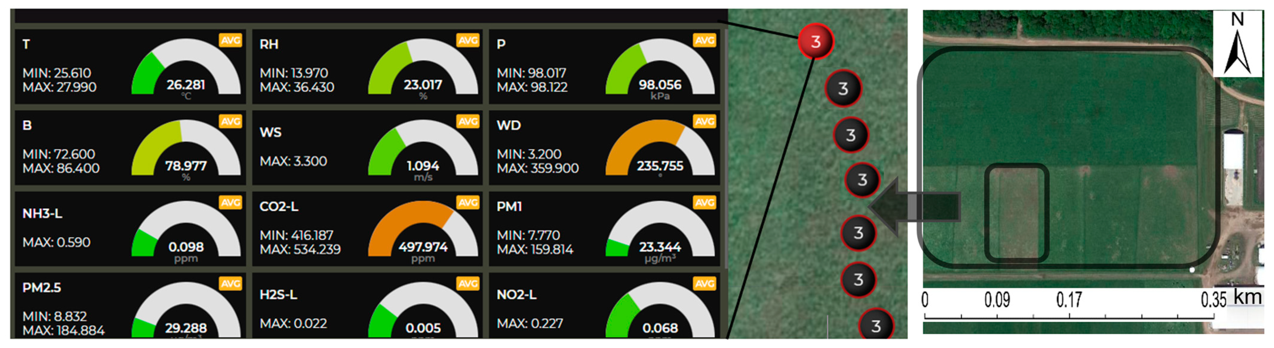
2.2. Test Site and Data Collection

Air samples were collected at the University of Wisconsin–Madison’s Marshfield Agricultural Research Station in Stratford, Wisconsin, U.S. The experimental site consisted of a 7.1 ha (17.55 acres) rotationally grazed dairy pasture, primarily composed of cool-season grasses with less than 30% legume content. The pasture was divided into 10 paddocks. A total of 18 “tester” heifers were placed on the pasture throughout the grazing season. The heifers were rotated twice a week, allowing each paddock a rest period of 28 to 30 days. The sample collection took place between late May and mid-July 2023.

Air samples were collected after fertilizer application (ammonium nitrate, NH₄NO₃, 33.5% N) and subsequently on a weekly basis (5 sampling days). A flight planning app (DJI GS Pro) was utilized to make sure flights were conducted at a constant speed (1 m s⁻¹) and height (1.5 m). This sampling speed and height were selected because they were the lowest speed and height at which the UAS could operate without disturbing the cows. About 1289 measurements were made per gas and particulate matter during each sampling day. The workflow of the study is shown in Figure S1.

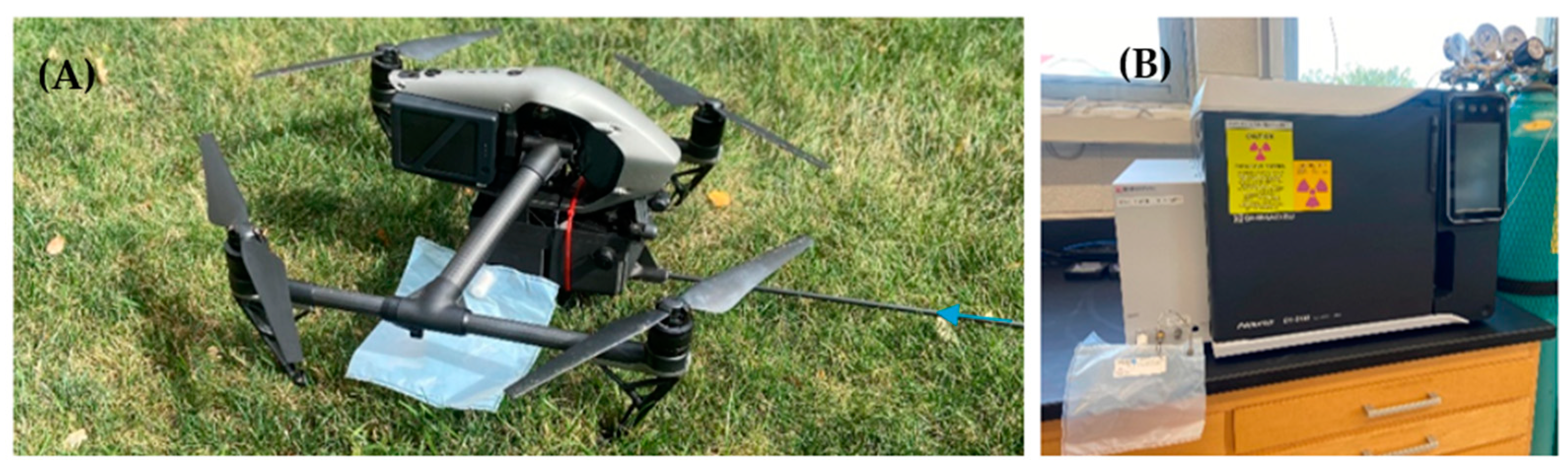
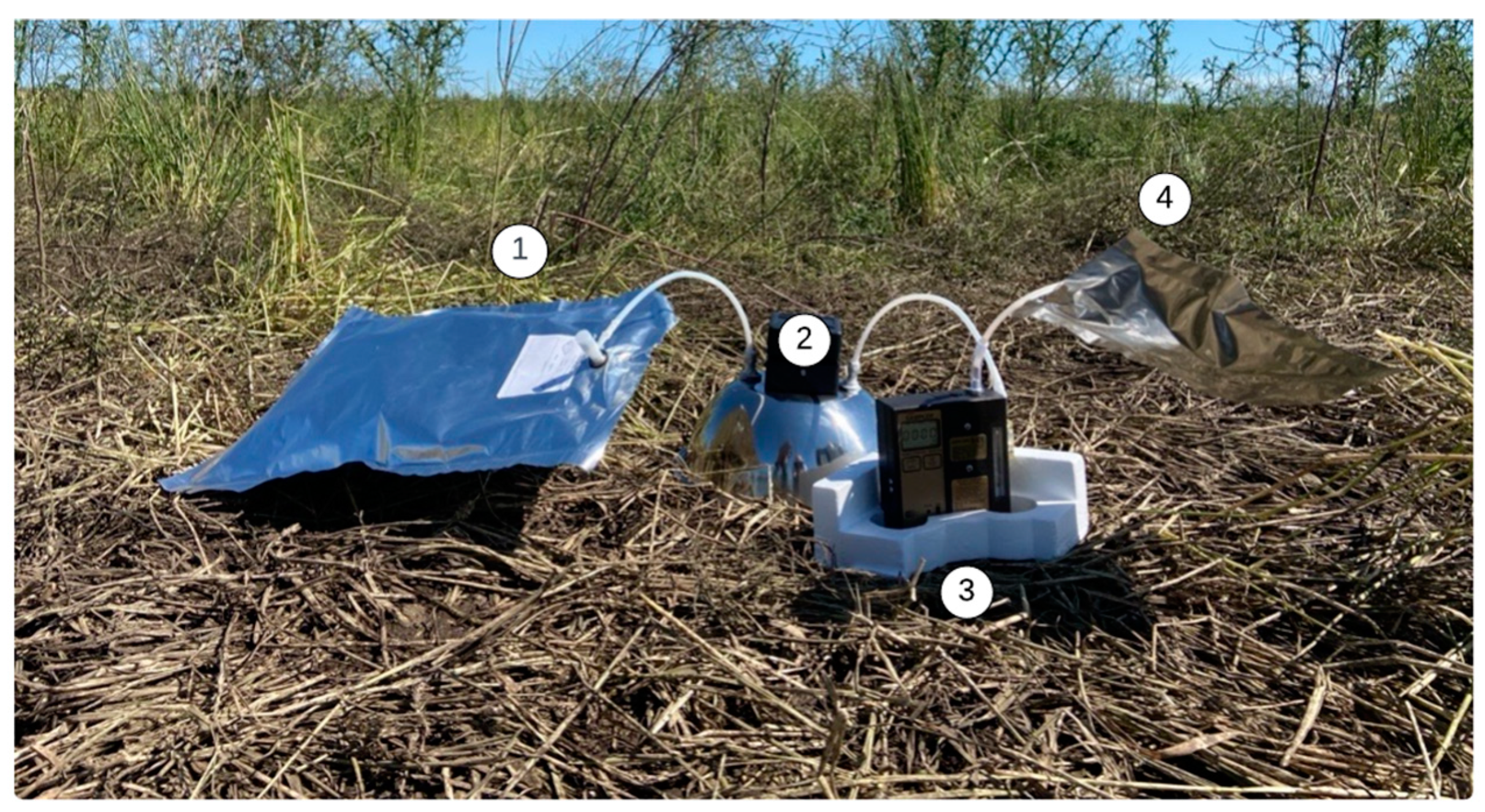
2.3. Sampling Bag Analysis

Prior to each sample collection, the sampling bags were flushed with ultra-high-purity nitrogen (Airgas, Pittsburgh, PA, USA) [25,26]. Two types of sampling bag experiments were conducted: (i) using the sample acquisition system, which allowed for remote sampling during flights (Figure 3), and (ii) using dynamic flux chambers (Figure 4). Dynamic flux chamber sampling is a standard sampling method, and it was conducted as described in previous studies [23]. In brief, ultra-high-purity nitrogen stored in a 10 L FlexFoil^® bag was delivered to the chamber (28 cm diameter) at an airflow rate of 1 L/min using an SKC air sampling pump (Universal PCXR8, SKC Inc., Eighty Four, PA, USA). The sample was collected in a 1 L FlexFoil^® bag. Before sampling, the entire system was flushed with nitrogen, and 400 g of weights were placed on the chamber to prevent tipping during sample collection [25,26].

The bags were analyzed on the same day the samples were collected using a GC2030 from Shimadzu Corp. (Kyoto, Japan) [27]. The instrument was equipped with a flame ionization detector (FID) and an electron capture detector (ECD). The column was divinylbenzene (30 m × 0.53 mm ID × 20 µm, Shimadzu, Kyoto, Japan). The injection port temperature was set at 100 °C. The oven temperature was initially set at 35 °C with 4.5 min holding time, followed by a ramp of 8 °C min⁻¹ until it reached 220 °C, where it was held for 5 min. The FID and ECD temperatures were set at 400 °C and 325 °C, respectively. LabSolutions version 5.117 was used for data acquisition and analysis. The column retention times were compared with those of GC-grade standards.

2.4. Data Analysis and Sensitivity Tests

DRIMS2 cloud software (version 4.1., Scentroid, Stouffville, Ontario, Canada) was used to download the DR2000 data. The concentrations were converted from ppm to g m⁻³ or mg m⁻³ using real-time temperature and atmospheric pressure measurements [13]. In the literature, two methods to calculate emission rates are reported: (i) Gaussian Plume Inversion (GPI) and (ii) the Lagrangian mass balance approach. The GPI approach is a method that estimates emission rates from point sources, specifically focusing on well-defined plumes. In this study, we used the mass balance approach because in the mass balance approach, the total input and output of a system are considered to estimate the emission rates, which is more suitable for diffuse sources, including pastures (Equation (1)) [2,13,16,28]:

$$ER={\int }_0^z{\int }_a^b(C_{ij}-C_0)V_{ij}dxdz$$

(1)

where $ER$ is the gas or particulate matter emission rate (g day⁻¹), ab is the plane perpendicular to the prevailing wind vector, $C_{ij}$ is the gas or particulate matter concentration (g m⁻³), $C_0$ is the measured background concentration (g m⁻³), $V_{ij}$ is the wind speed (m day⁻¹), and $dx$ and $dz$ are the horizontal and the vertical increments of the integration plane (m), respectively. Once the emission rates per day were calculated, they were divided by the area of the paddock (0.71 ha) to obtain emission rates in g day⁻¹ m⁻².

ArcGIS Pro version 3.1.0 (ESRI Inc., Redlands, CA, USA) was used for spatial Kriging interpolation and preparing emission maps. The latitude of the pasture ranged from 44°45′42″N to 44°45′46″N, and the longitude ranged from 90°6′20″W to 90°6′28″W. Sensitivity analyses were conducted by testing six “number of points” (25, 50, 75, 100, 125, 150) and four semi-variogram models (spherical, circular, exponential, and gaussian). The average standard deviations were calculated using the coefficient of variance (Equations (2) and (3)) [29]. All statistical analyses were performed using Origin Pro 2024 (OriginLab Corporation, Northampton, MA, USA). The means were compared using a Tukey HSD test at a 5% significance level.

$$Averagestandarddeviation=\sqrt{{\displaystyle \frac{({s1}^2+{s2}^2+\dots {s5}^2)}{5}}}$$

(2)

where $s$ is the standard deviation for a particular sampling day.

$$Coefficientofvariance(CV,\%)={\displaystyle \raisebox{1ex}{$\sigma $}\!\left/ \!\raisebox{-1ex}{$\mu $}\right.}$$

(3)

where $\sigma$ is the standard deviation and $\mu$ is the mean.

3. Results

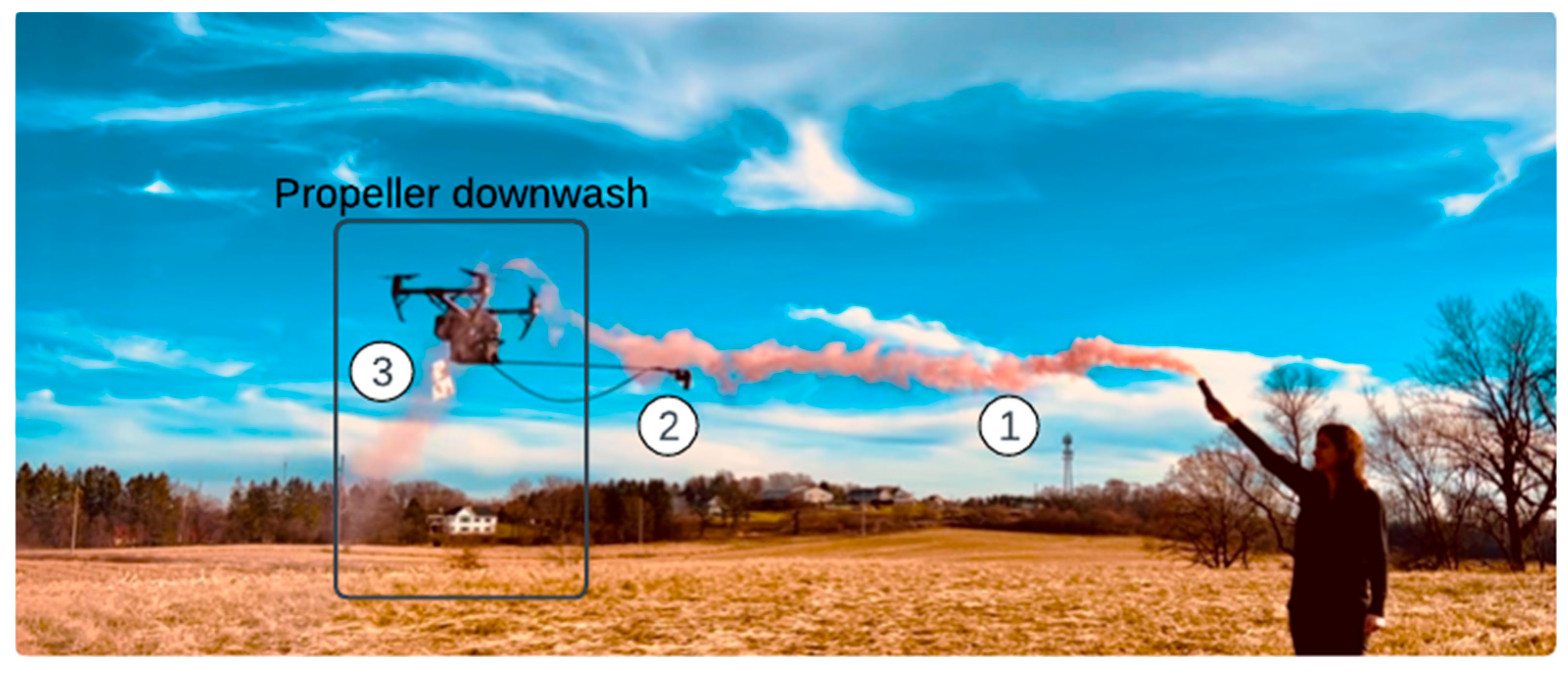
3.1. Propeller Downwash

A major concern with UAS-based sampling is the possible impact of the vertical airflow generated by the propellers (i.e., downwash) on the measurements. To collect air samples from an undisturbed area, we utilized an 88 cm long horizontal sampling probe. As shown in Figure 5 our colored smoke test visually demonstrated that the sampling probe was long enough to avoid downwash from the DJI Inspire II when it was oriented upwind. This is not the only study that has documented downwash using the colored smoke test. Crazzolara et al. [30] also conducted a similar smoke test focusing on visualizing the aerodynamic characteristics of the downwash generated by rotorcrafts. Although a sampling probe was not used in that study, the results visually demonstrated that a probe similar to the one used in our study would have helped to avoid the downwash of a hovering DJI Matrice 600 during chemical sensing. There are also studies in the literature that focus on modeling downwash using computational fluid dynamics [31,32]. While these studies are valuable, in some cases, gas and environmental properties are not considered, and the models are developed under general conditions to present the feasibility of using CFD to simulate downwash [32]. However, pastures have a dynamic and variable environment, and environmental conditions vary widely. In this study, the smoke test clearly demonstrated how propeller downwash affects airflow patterns [30,31] and highlighted the importance of positioning the sampling probe upwind to minimize the disruption to the air samples.

3.2. Kriging Interpolation and Sensitivity Analysis

The results from the sensitivity tests for Kriging interpolation are presented in Figure 6A, B. The advantage of Kriging interpolation is that it calculates the spatial correlation between measurement points and quantifies uncertainties from the spatial variability of data density [33]. As shown in Figure 6A, the coefficient of variation of the data at 100 “number of points” decreased below 40%. Lower coefficient of variance values suggested that less variation in the emission rates (lower error of prediction) was achieved at 100 and a higher “number of points”. The default setting for Kriging interpolation is 12 “number of points”, but Oliver and Webster [34] recommended a minimum of 100 “number of points”, which is consistent with the findings of our study.

Figure 6B shows the coefficient of variance for semivariogram models at 100 “number of points”. Although the coefficient of variance did not vary much among the models (average CV range: 22.7–26.0%), since the lowest coefficient of variance (on average 22.7%) was achieved with the spherical model, this model was chosen to be used in the analysis. Zhang et al. [35] also reported that the spherical model was the theoretical model with the best-fitting effect for the spatial-temporal Kriging interpolation.

3.3. Gas Chromatography Analysis and Quality Control

Air sampling bags gathered during the flights were analyzed for CO₂, CH₄, and N₂O. The chromatographs of the laboratory air samples are presented in Figure S2 as a quality control measure. Sharp peaks in the chromatogram and the ability to detect gasses at atmospheric levels (CO₂: 433.5 ± 21.6 ppm, CH₄: 1.97 ± 0.08 ppm, N₂O: 0.38 ± 0.02 ppm) indicated high sensitivity of the detectors. The samples collected during the flights had average CO₂, CH₄, and N₂O concentrations of 465 ± 23.1 ppm (800 ± 39.7 mg m⁻³), 2.2 ± 0.1 ppm (1.38 ± 0.063 mg m⁻³), and 0.410 ± 0.02 ppm (0.71 ± 0.03 mg m⁻³), respectively. For CO₂, there was no significant difference between the DR2000 sensor and GC measurements (p = 0.061). The CO₂ levels were within the 1% range. CH₄ and N₂O DR2000 readings were inconsistent because the CH₄ sensor was not sensitive enough for low-level measurements, and the response time of the N₂O sensor was too long for UAS-based sampling (>10 s). Although we could not interpolate data for CH₄ and N₂O measurements, we were still able to detect average concentrations using the sample acquisition system, which allowed for remote bag sampling during the flights and analysis in the laboratory using GC.

Dynamic flux chamber measurements provided information about ground-level emission rates (n = 5). The average ground-level CO₂, CH₄, and N₂O concentrations were 581 ± 31 ppm (1000 ± 53.3 mg m⁻³), 2.75 ± 0.14 ppm (1.73 ± 0.09 mg m⁻³), and 0.42 ± 0.02 ppm (0.73 ± 0.04 mg m⁻³), respectively. While the CO₂ and CH₄ levels were about 25% greater at the ground level compared to the 1 m height, N₂O concentrations were 2.8% higher. Although it was beyond the scope of this study, atmospheric dispersion models could be developed by including more measurement heights. These models would provide valuable insights into the behavior and distribution of greenhouse gasses across different altitudes.

3.4. Gas and Particulate Matter Concentrations

The DRIMS2 software (version 4.1., Scentroid, Stouffville, ON, Canada) recorded the minimum, maximum, and average concentrations of the gasses (CO₂, CH₄, NH₃, H₂S, NO₂, and TVOCs) and particulate matters (PM₁, PM_2.5, PM₁₀), as well as temperature, relative humidity, barometric pressure, wind speed, and direction. Figure 7 shows a snapshot from the software to demonstrate that the sampling occurred along a relatively straight line and at a constant speed, with three samples collected at each stop. Considering UAS flights can be unsteady [36,37], this indicates the stability achieved during our analysis.

Our results indicated that the 5-sampling-day average weather temperature was 27.9 ± 4.8 °C, within the average temperature range (23.8–29.4 °C) for Wisconsin [38]. The average wind speed was 1.4 ± 3.7 m s⁻¹, and the wind was blowing from a direction of 225°, indicating a southwest direction, which is typical for Wisconsin during the summer. The cows were comfortable with having a UAS around. They continued their daily routines while sample collection was ongoing. This observation was important because if there had been increased activity, it would have affected the emission rates.

The 5-sampling-day average CO₂ concentrations (463 ± 32.2 ppm) were slightly higher than the typical atmospheric CO₂ levels (417–424 ppm) [39]. Depending on the sampling time, the NH₃ concentrations varied from 110 to 520 ppb (atmospheric levels: 50 ppt–5 ppb) [40], while the H₂S concentrations were around 10 ± 2 ppb (atmospheric levels: 0.1–0.5 ppb) [41].

While particulate matter (PM₁, PM_2.5, PM₁₀) is not a gas, it still contributes to warming or cooling effects on the climate [42]. We detected considerable amounts of PM₁ (23.1 ± 5.2 µg m⁻³), PM_2.5 (28.1 ± 13.3 µg m⁻³), and PM₁₀ (33.1 ± 15.0 µg m⁻³) during our sampling collection. The concentrations of PM_2.5 and PM₁₀ were above the annual average values set by the California ambient air quality standards, which are 12 µg m⁻³ for PM_2.5 and 20 µg m⁻³ for PM₁₀ [43]. On 7 February 2024, the Environmental Protection Agency strengthened the particulate matter National Ambient Air Quality Standards, setting the PM_2.5 standard at 9.0 µg m⁻³ to provide increased public health protection [44].

Total VOCs and NO₂ are considered to be indirect GHGs. Total VOCs were within the range of 0.7 ± 0.3 ppm, which is the level recommended by the US EPA for good air quality [45]. However, the average NO₂ concentrations were 20% over the US EPA’s annual NO₂ standard [46].

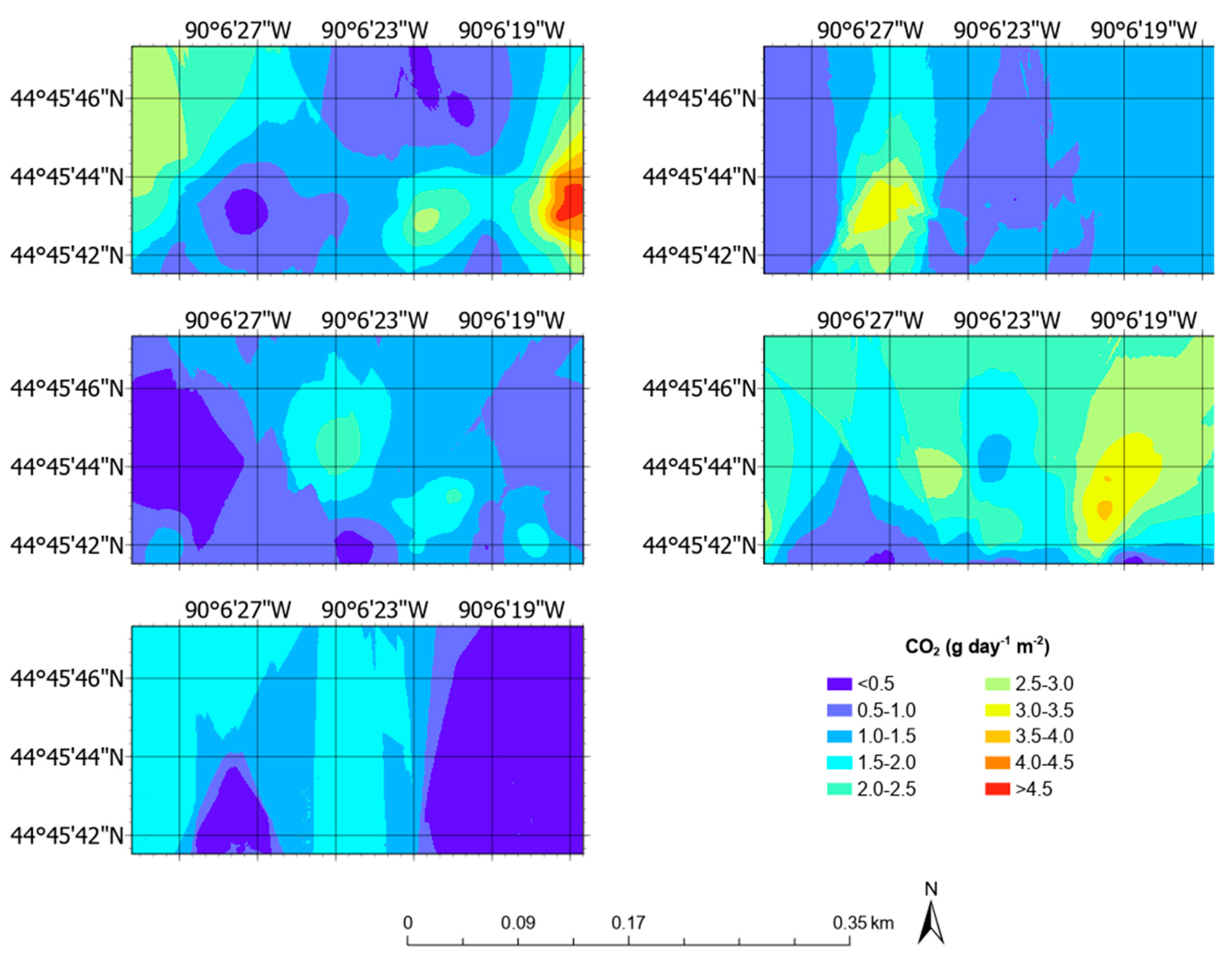
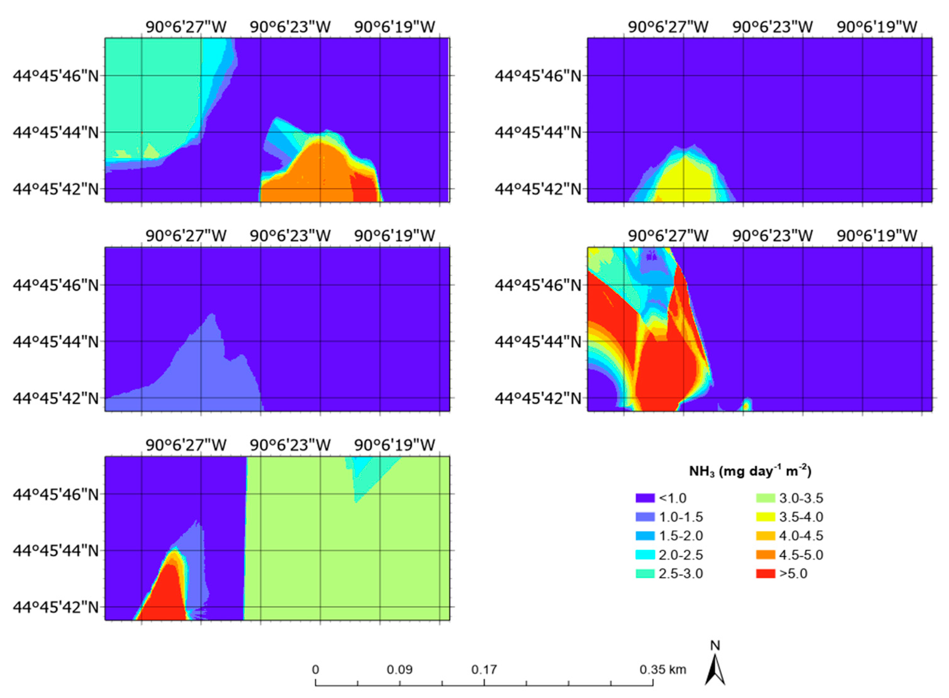
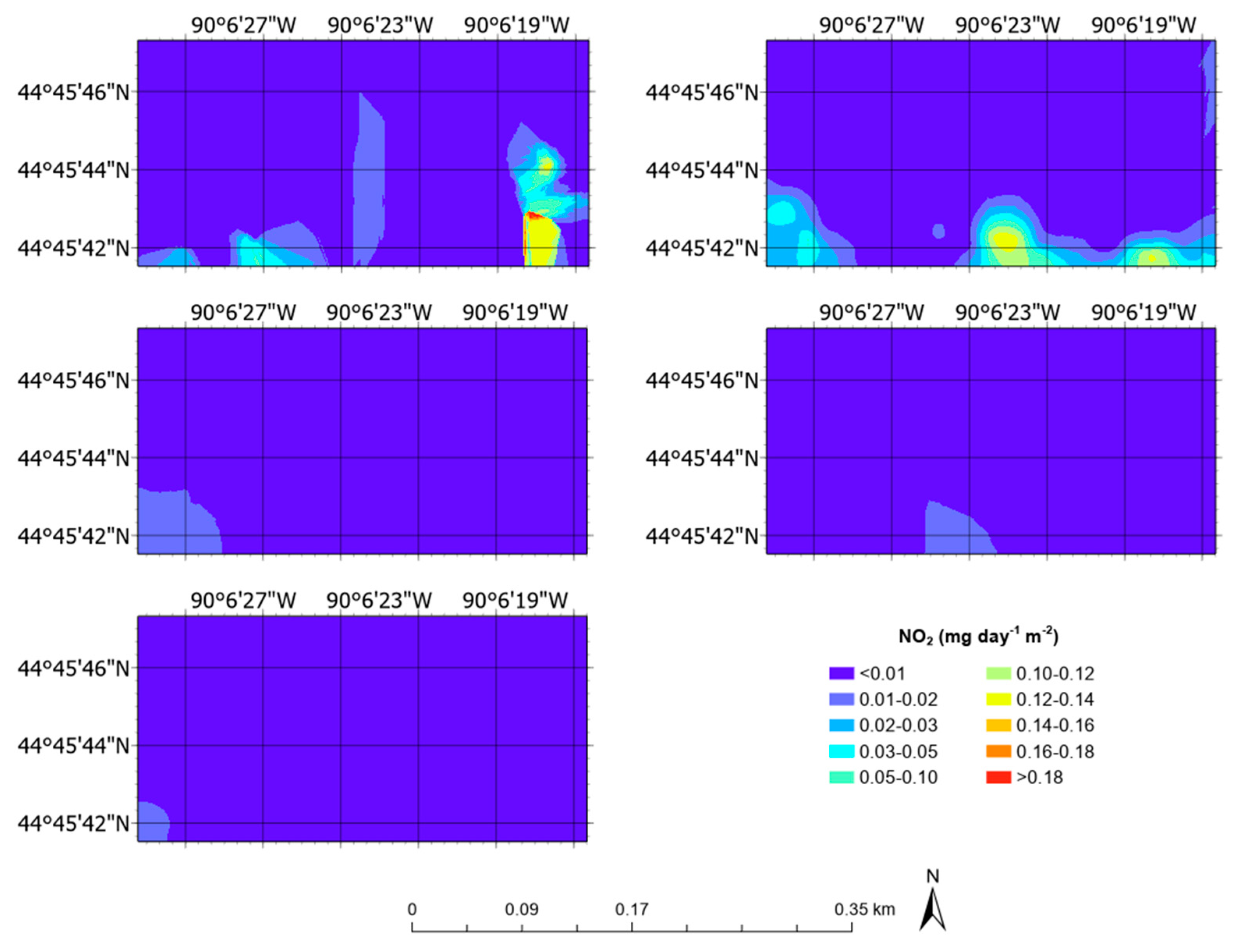
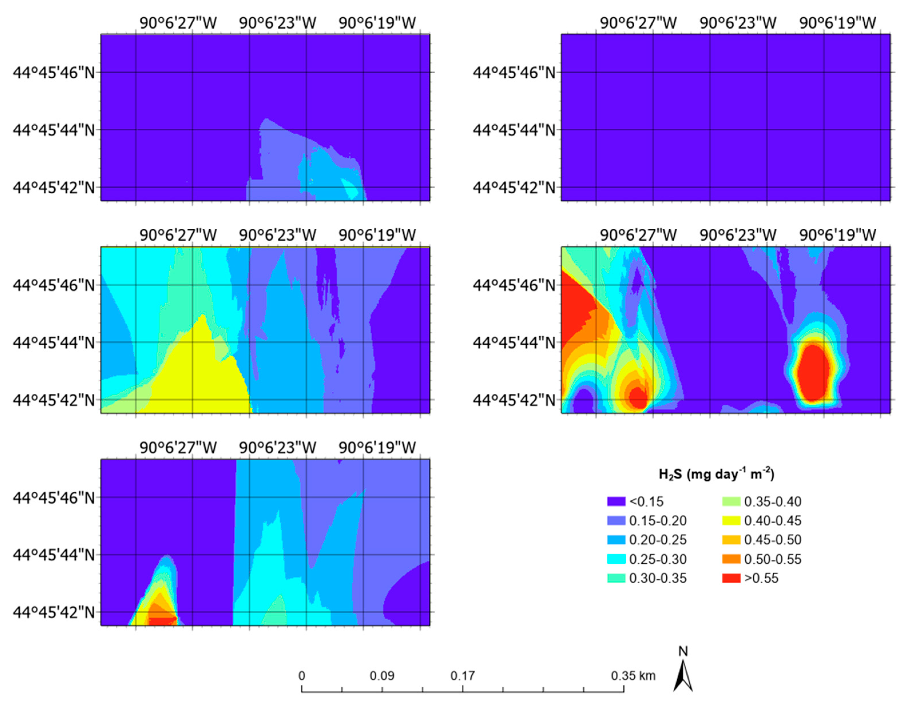
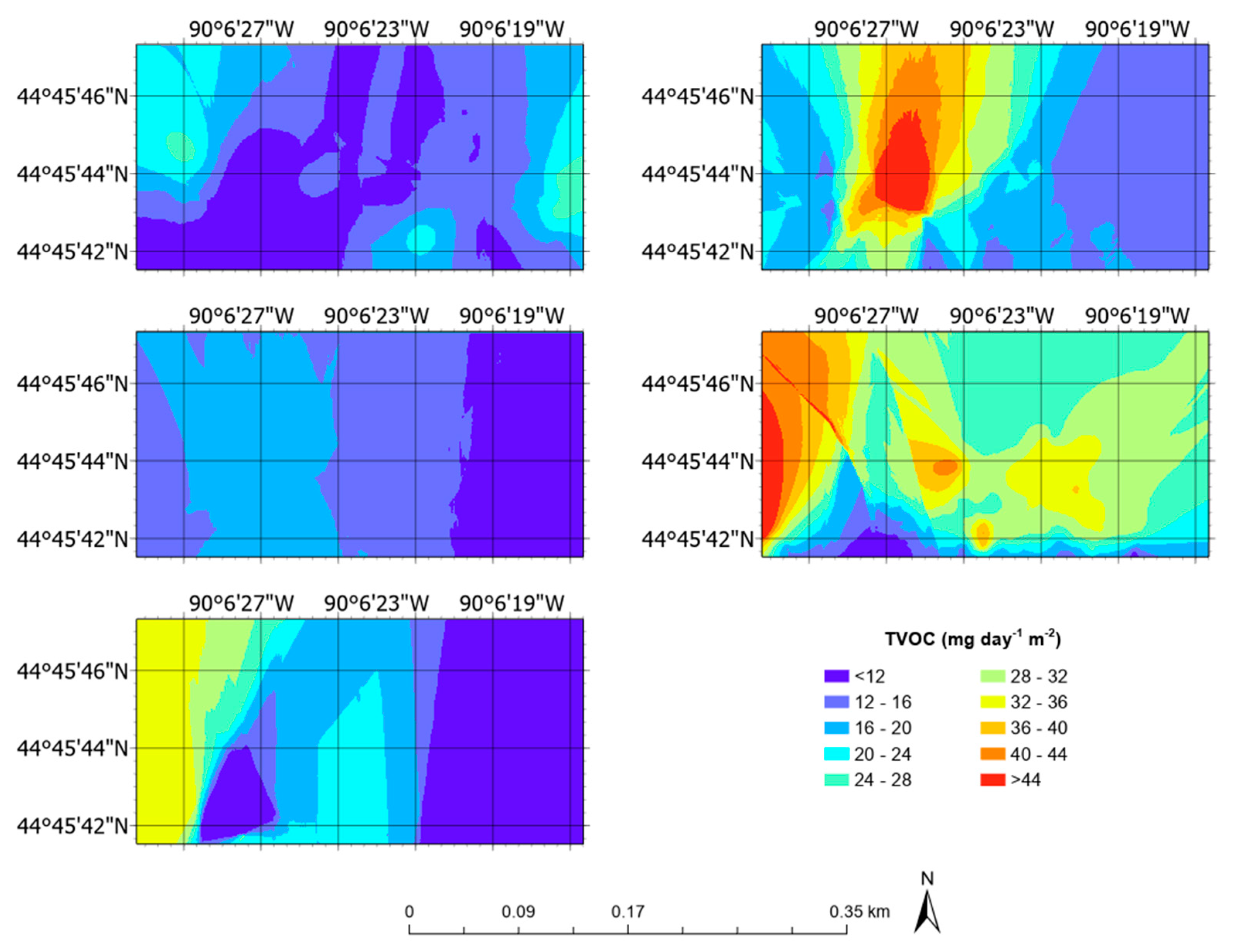
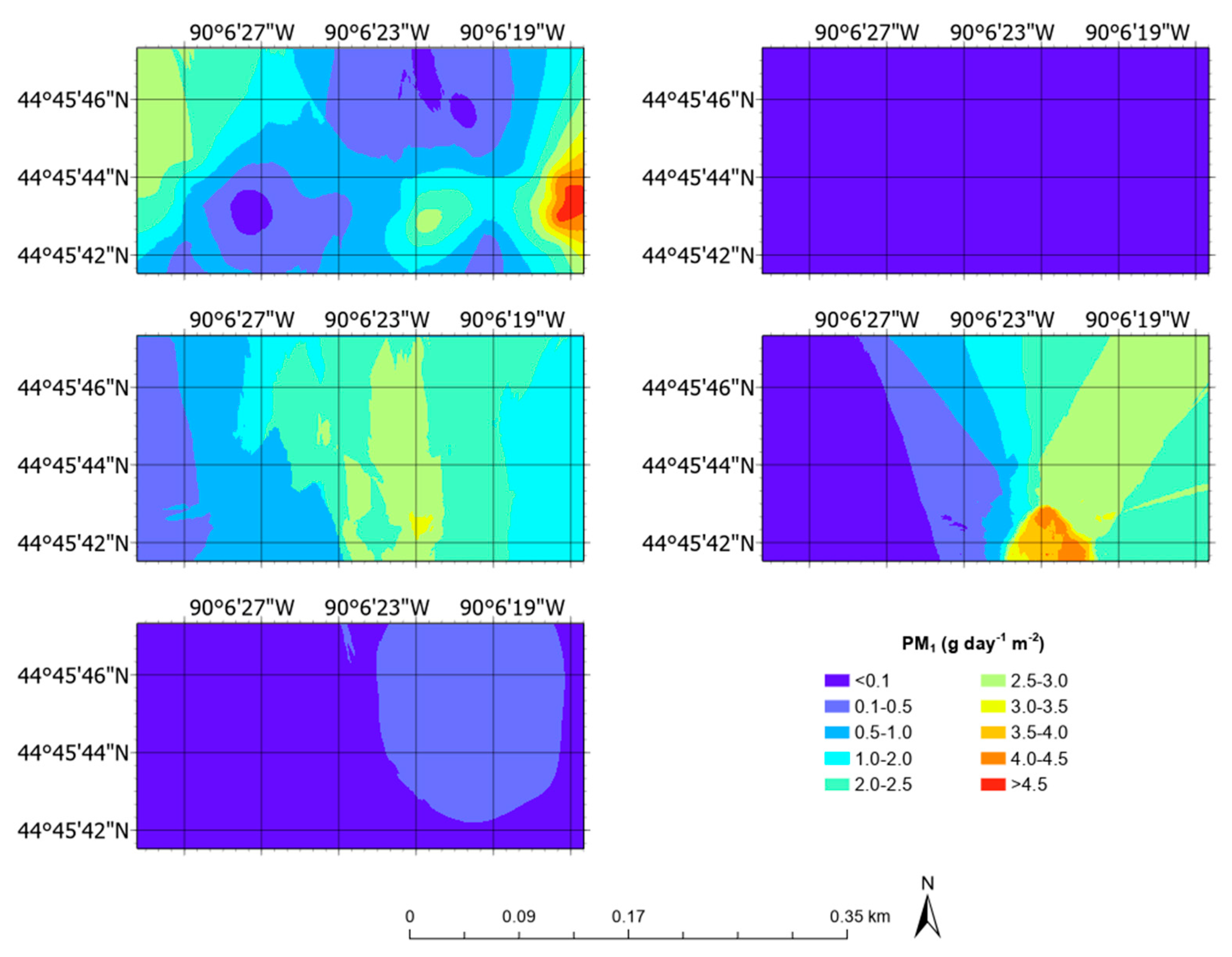
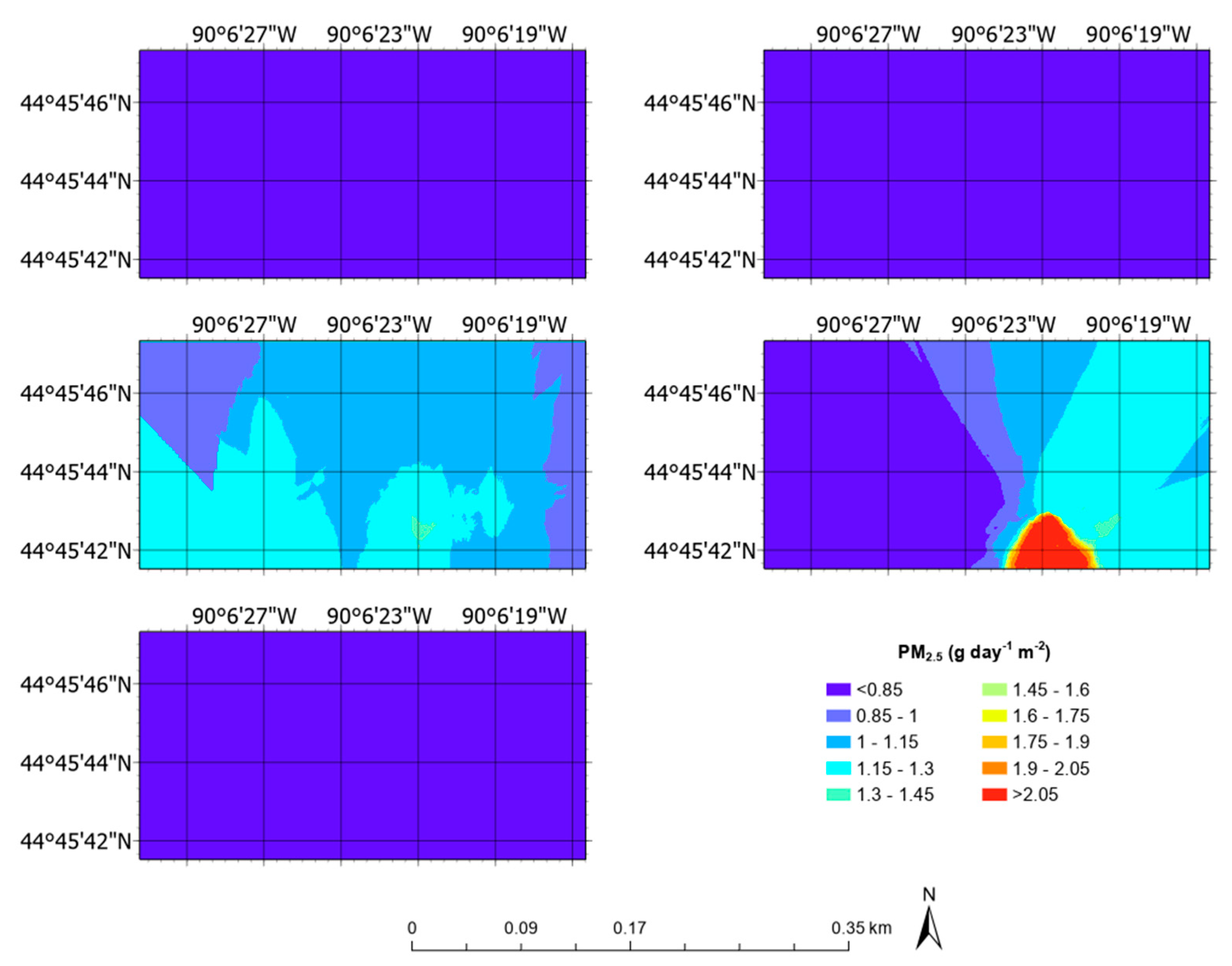
3.5. Aerial Emission Rate Maps

Kriging interpolation and emission maps are shown in Figure 8, Figure 9, Figure 10, Figure 11, Figure 12, Figure 13, Figure 14 and Figure 15. The emission rates varied across the 7.1 ha pasture (Figure 8, Figure 9, Figure 10, Figure 11, Figure 12, Figure 13, Figure 14 and Figure 15 and

Table 2. Estimation of spatial emission rates using Kriging interpolation (n = 124,500 per gas/PM).

Compound	Unit	Mean ± Stdev	Lower Bound	Upper Bound
CO2	g day−1 m−2	1.52 ± 0.80	0.25	4.64
NH3	mg day−1 m−2	1.22 ± 1.02	0.00	6.60
NO2	mg day−1 m−2	0.01 ± 0.01	0.00	0.09
H2S	mg day−1 m−2	0.08 ± 0.05	0.01	0.46
TVOC	mg day−1 m−2	14.23 ± 4.71	3.70	25.73
PM1	g day−1 m−2	0.14 ± 0.04	0.00	5.02
PM2.5	g day−1 m−2	0.11 ± 0.03	0.04	0.20
PM10	g day−1 m−2	0.04 ± 0.02	0.01	0.14

), highlighting the importance of surveying the entire surface of the pasture when measuring air emissions rather than collecting grab samples. Saggar et al. [47] also reported that emission rates varied according to the sampling location and day. One of the reasons for the varying emission rates across the pasture was due to the location of the grazing cows. The pasture was rotationally grazed, and the cows were moved to a different location each sampling day. About eight to nine times higher NH₃ and H₂S emissions were detected in the areas where fresh manure was deposited by the cows, which was expected, as reported in other studies [48,49]. Another potential factor influencing emission rates might be the homogeneity of the fertilizer application [50]. Additionally, tractor traffic near the roadside might have affected the emission rates of PM_2.5, PM₁₀, and NO₂ [51]. CO₂ emissions are often linked to pasture management and yields [52]. Pasture itself and manure are known to be sources of total VOC emissions [53]. However, no information regarding total VOC emissions from dairy pastures has been provided in the literature.

4. Discussion

While many factors affect emission rates, the average CO₂ emission rate was 1.52 ± 0.80 g day⁻¹ m⁻² (Table 2), which was within the range reported by Bento et al. [54]. Bento, Brandani [54] measured CO₂ emission rates from livestock pastures using static flux chambers and reported the average rate to be 2.11 ± 0.25 g day⁻¹ m⁻² following mineral fertilizer application. In another study, CO₂ emission rates from pastures were reported to be 3.81 g day⁻¹ m⁻² [55]. However, the emission rates varied depending on the intensity of the grazing. Weather and soil conditions are also known to affect CO₂ emission rates [56].

As expected, the NH₃ and H₂S emission rates were much lower compared to the CO₂ emission rates (NH₃ 1.22 ± 1.02 mg day⁻¹ m⁻²; H₂S: 0.08 ± 0.05 mg day⁻¹ m⁻²) (Table 2). Manure is known to be the main source of these emissions [57]. For ammonia, emission rates ranging from 0.42 to 250 g per day per cow have been reported in the literature [58]. In this study, ammonia emission rates were on the lower end of this spectrum (0.48 g per day per cow). The lower NH₃ emission rates were likely due to the fact that there were 18 cows on the pasture. Considerable amounts of particulate matter emissions were measured (PM₁: 0.14 ± 0.04; PM_2.5: 0.11 ± 0.03; PM₁₀: 0.04 ± 0.02 g day⁻¹ m⁻²). McGinn et al. [59] reported mean PM₁₀ emission rates from cattle feedlots in Australia at 10 µg m⁻² s⁻¹. Considering that the stocking rate in that study was 20 m² per animal, compared to 394 m² per animal in this study, this emission rate was equivalent to 0.04 g day⁻¹ m⁻². Although particulate matter emissions are related to fertilizer application and cow activity, vehicles around the pasture could have contributed to these emissions [60].

This study aimed to develop a method for directly measuring air emissions from dairy pastures, addressing a significant gap in the literature. In this study, ground-level concentrations were measured using dynamic flux chambers. The next phase of this research will involve collecting air samples at various heights to model the dispersion of gasses and particulate matter plumes. A laboratory-scale model for PM₁₀ was previously reported, but it was not validated under real atmospheric conditions [61]. Additionally, while split fertilizer applications are known to reduce NO_x and N₂O emissions [49], there is insufficient understanding of how pasture and soil conditions may affect their emissions. Future studies will include comprehensive pasture and soil characterization.

5. Conclusions

In this study, we used a UAS-based sampling method to prepare air emission maps for a rotationally grazed dairy pasture. It was demonstrated that using an 88 cm sampling probe prevented propeller downwash from affecting the measurements. Kriging interpolation sensitivity tests showed that a lower prediction error was achieved with 100 “number of points” (CV < 40%). The UAS system’s sample acquisition system allowed remote bag sampling during flights. The bag samples collected had average CO₂, CH₄, and N₂O concentrations of 465 ± 23.1 ppm (800.1 ± 39.7 mg m⁻³), 2.2 ± 0.1 ppm (1.38 ± 0.063 mg m⁻³), and 0.410 ± 0.02 ppm (0.71 ± 0.03 mg m⁻³), respectively. The CO₂ levels were within the 1% range, and there was no significant difference between the DR2000 sensor and GC sampling (p < 0.001). Using the mass balance model combined with Kriging interpolation, CO₂ emission rates were estimated at 1.52 ± 0.80 g day⁻¹ m⁻², which fell within the range reported in the literature using static flux chambers. Future studies could focus on measuring air emissions at different altitudes, and additional information related to the pastures could also be included.

References

1. FAA. Small Unmanned Aircraft System (sUAS). Available online: https://www.faa.gov/air_traffic/publications/atpubs/aim_html/chap11_section_2.html (accessed on 17 April 2024).
2. Vinkovic, K.; Andersen, T.; De Vries, M.; Kers, B.; Van Heuven, S.; Peters, W.; Hensen, A.; Van Den Bulk, P.; Chen, H. Evaluating the use of an unmanned aerial vehicle (UAV)-based active AirCore system to quantify methane emissions from dairy cows. Sci. Total Environ. 2022, 831, 154898. [Google Scholar] [CrossRef] [PubMed]
3. Burgués, J.; Esclapez, M.D.; Doñate, S.; Pastor, L.; Marco, S. Aerial mapping of odorous gases in a wastewater treatment plant using a small drone. Remote Sens. 2021, 13, 1757. [Google Scholar] [CrossRef]
4. Arroyo, P.; Gómez-Suárez, J.; Herrero, J.L.; Lozano, J. Electrochemical gas sensing module combined with unmanned aerial vehicles for air quality monitoring. Sens. Actuators B Chem. 2022, 364, 131815. [Google Scholar] [CrossRef]
5. Bakirci, M. Efficient air pollution mapping in extensive regions with fully autonomous unmanned aerial vehicles: A numerical perspective. Sci. Total Environ. 2023, 909, 168606. [Google Scholar] [CrossRef] [PubMed]
6. Bax, C.; Sironi, S.; Capelli, L. How can odors be measured? An overview of methods and their applications. Atmosphere 2020, 11, 92. [Google Scholar] [CrossRef]
7. Burgués, J.; Doñate, S.; Esclapez, M.D.; Saúco, L.; Marco, S. Characterization of odour emissions in a wastewater treatment plant using a drone-based chemical sensor system. Sci. Total Environ. 2022, 846, 157290. [Google Scholar] [CrossRef] [PubMed]
8. Schellenberg, B.; Richardson, T.; Watson, M.; Greatwood, C.; Clarke, R.; Thomas, R.; Wood, K.; Freer, J.; Thomas, H.; Liu, E.; et al. Remote sensing and identification of volcanic plumes using fixed-wing UAVs over Volcán de Fuego, Guatemala. J. Field Robot. 2019, 36, 1192–1211. [Google Scholar] [CrossRef]
9. Burgues, J.; Marco, S. Environmental chemical sensing using small drones: A review. Sci. Total Environ. 2020, 748, 141172. [Google Scholar] [CrossRef]
10. Rutkauskas, M.; Asenov, M.; Ramamoorthy, S.; Reid, D.T. Autonomous multi-species environmental gas sensing using drone-based Fourier-transform infrared spectroscopy. Opt. Express 2019, 27, 9578–9587. [Google Scholar] [CrossRef]
11. Emran, B.; Tannant, D.; Najjaran, H. Low-Altitude Aerial Methane Concentration Mapping. Remote Sens. 2017, 9, 823. [Google Scholar] [CrossRef]
12. Roldan, J.J.; Garcia-Aunon, P.; Garzon, M.; De Leon, J.; Del Cerro, J.; Barrientos, A. Heterogeneous multi-robot system for mapping environmental variables of greenhouses. Sensors 2016, 16, 1018. [Google Scholar] [CrossRef] [PubMed]
13. Galfalk, M.; Nilsson Paledal, S.; Bastviken, D. Sensitive drone mapping of methane emissions without the need for supplementary ground-based measurements. ACS Earth Space Chem. 2021, 5, 2668–2676. [Google Scholar] [CrossRef]
14. Ali, N.B.H.; Abichou, T.; Green, R. Comparing estimates of fugitive landfill methane emissions using inverse plume modeling obtained with surface emission monitoring (SEM), drone emission monitoring (DEM), and downwind plume emission monitoring (DWPEM). J. Air Waste Manag. Assoc. 2020, 70, 410–424. [Google Scholar] [CrossRef]
15. Yuan, H.; Xiao, C.; Wang, Y.; Peng, X.; Wen, Y. Maritime vessel emission monitoring by a UAV gas sensor system. Ocean Eng. 2020, 218, 108206. [Google Scholar] [CrossRef]
16. Allen, G.; Hollingsworth, P.; Kabbabe, K.; Pitt, J.R.; Mead, M.I.; Illingworth, S.; Roberts, G.; Bourn, M.; Shallcross, D.E.; Percival, C.J. The development and trial of an unmanned aerial system for the Measurement of methane flux from landfill and greenhouse gas emission hotspots. Waste Manag. 2019, 87, 883–892. [Google Scholar] [CrossRef]
17. Kearney, M.; O’Riordan, E.G.; Byrne, N.; Breen, J.; Crosson, P. Mitigation of greenhouse gas emissions in pasture-based dairy-beef production systems. Agric. Syst. 2023, 211, 103748. [Google Scholar] [CrossRef]
18. Munidasa, S.; Eckard, R.; Sun, X.; Cullen, B.; McGill, D.; Chen, D.; Cheng, L. Challenges and opportunities for quantifying greenhouse gas emissions through dairy cattle research in developing countries. J. Dairy Res. 2021, 88, 3–7. [Google Scholar] [CrossRef] [PubMed]
19. Pas, M.A.W.; Uddin, M.E.; Letelier, P.; Jackson, R.D.; Larson, R.A. Emission and Mitigation of greenhouse gases from dairy farms: The cow, the manure, and the field. Appl. Anim. Sci. 2019, 35, 238–254. [Google Scholar] [CrossRef]
20. Reinemann, D.J.; Larson, R.; Aguirre-Villegas, H.; Passos-Fonseca, T. Comparing Greenhouse Gas Emissions of Dairy Systems. Available online: https://cias.wisc.edu/wp-content/uploads/sites/194/2019/03/ciasrb101final.pdf (accessed on 14 February 2024).
21. Rotz, C.A. Modeling greenhouse gas emissions from dairy farms. J. Dairy Sci. 2018, 101, 6675–6690. [Google Scholar] [CrossRef]
22. Collier, S.M.; Ruark, M.D.; Oates, L.G.; Jokelam, W.E.; Dell, C.J. Measurement of greenhouse gas flux from agricultural soils using static chambers. J. Vis. Exp. 2014, 90, 52110. [Google Scholar] [CrossRef]
23. Pape, L.; Ammann, C.; Nyfeler-Brunner, A.; Spirig, C.; Hens, K.; Meisinger, F.X. An automated dynamic chamber system for surface exchange measurement of non-reactive and reactive trace gases of grassland ecosystems. Biogeosciences 2009, 6, 405–429. [Google Scholar] [CrossRef]
24. ISO 21501-4; Determination of Particle Size Distribution—Single Particle Light Interaction Methods. 2023. Available online: https://www.en-standard.eu/bs-iso-21501-4-2018-a1-2023 (accessed on 12 August 2024).
25. Akdeniz, N.; Janni, K.A.; Hetchler, B.P. Mitigation of multiple air emissions from swine buildings using corn cob biofilters. Trans. ASABE 2016, 59, 1413–1420. [Google Scholar] [CrossRef]
26. Akdeniz, N.; Janni, K.A.; Salnikov, I.A. Biofilter performance of pine nuggets and lava rock as media. Bioresour. Technol. 2011, 102, 4974–4980. [Google Scholar] [CrossRef] [PubMed]
27. Sun, Z.; Akdeniz, N.; Banik, C.; Koziel, J.A. Alkaline hydrolysis of poultry carcasses and health risk assessment of exposure to target volatile organic compounds. J. ASABE 2024, 67, 373–384. [Google Scholar] [CrossRef]
28. Nathan, B.J.; Golston, L.M.; O’Brien, A.S.; Ross, K.; Harrison, W.A.; Tao, L.; Lary, D.J.; Johnson, D.R.; Covington, A.N.; Clark, N.N.; et al. Near-Field Characterization of methane emission variability from a compressor station using a model aircraft. Environ. Sci. Technol. 2015, 49, 7896–7903. [Google Scholar] [CrossRef] [PubMed]
29. Khan, S.H. International Encyclopedia of Statistical Science-Standard Deviation; Springer: Berlin/Heidelberg, Germany, 2014. [Google Scholar]
30. Crazzolara, C.; Ebner, M.; Platis, A.; Miranda, T.; Bange, J.; Junginger, A. A new multicopter-based unmanned aerial system for pollen and spores collection in the atmospheric boundary layer. Atmos. Meas. Tech. 2019, 12, 1581–1598. [Google Scholar] [CrossRef]
31. Burgues, J.; Hernandez, V.; Lilienthal, A.J.; Marco, S. Smelling nano aerial vehicle for gas source localization and mapping. Sensors 2019, 19, 478. [Google Scholar] [CrossRef] [PubMed]
32. Luo, B.; Meng, Q.H.; Wang, J.Y.; Ma, S.G. Simulate the aerodynamic olfactory effects of gas-sensitive UAVs: A numerical model and its parallel implementation. Adv. Eng. Softw. 2016, 102, 123–133. [Google Scholar] [CrossRef]
33. Cosentino, N.J.; Opaza, N.E.; Lambert, F.; Osses, A.; Van Wout, E. Global-Krigger: A global Kriging interpolation toolbox with paleoclimatology examples. Adv. Earth Space Sci. 2023, 24, e2022GC010821. [Google Scholar] [CrossRef]
34. Oliver, M.A.; Webster, R. The Variogram and Modelling. In Basic Steps in Geostatistics: The Variogram and Kriging; Oliver, M.A., Webster, R., Eds.; Springer International Publishing: Cham, Switzerland, 2015; pp. 15–42. [Google Scholar]
35. Zhang, H.; Tian, Y.; Zhao, P. Dispersion curve interpolation based on Kriging method. Appl. Sci. 2023, 13, 2557. [Google Scholar] [CrossRef]
36. Darvishpoor, S.; Roshanian, J.; Raissi, A.; Hassanalian, M. Configurations, flight mechanisms, and applications of unmanned aerial systems: A review. Prog. Aerosp. Sci. 2020, 121, 100694. [Google Scholar] [CrossRef]
37. Hassanalian, M.; Abdelkefi, A. Classifications, applications, and design challenges of drones: A review. Prog. Aerosp. Sci. 2017, 91, 99–131. [Google Scholar] [CrossRef]
38. WSCO. Summer Climate Data-Wisconsin State Climatology Office. Available online: https://climtology.nelson.wisc.edu/wisconsin-seasons/summer/ (accessed on 14 March 2024).
39. NOAA. Climate Change: Atmospheric Carbon Dioxide. Available online: https://www.climate.gov/news-features/understanding-climate/climate-change-atmospheric-carbon-dioxide (accessed on 14 May 2024).
40. Li, M.; Weschler, C.J.; Bekö, G.; Wargocki, P.; Lucic, G.; Williams, J. Human ammonia emission rates under various indoor environmental conditions. Environ. Sci. Technol. 2020, 54, 5419–5428. [Google Scholar] [CrossRef] [PubMed]
41. ATSDR. Public Health Statement Hydrogen Sulfide. Available online: https://www.atsdr.cdc.gov/ToxProfiles/tp114-c1-b.pdf (accessed on 14 March 2024).
42. EPA. Air Quality and Climate Change Research. Available online: https://www.epa.gov/air-research/air-quality-and-climate-change-research (accessed on 14 March 2024).
43. CAAQS. California Ambient Air Quality Standards. Available online: https://ww2.arb.ca.gov/resources/inhalable-particulate-matter-and-health (accessed on 16 September 2023).
44. EPA. National Ambient Air Quality Standards (NAAQS) for PM. Available online: https://www.epa.gov/pm-pollution/national-ambient-air-quality-standards-naaqs-pm (accessed on 7 May 2024).
45. EPA. Technical Overview of Volatile Organic Compounds. Available online: https://www.epa.gov/indoor-air-quality-iaq/technical-overview-volatile-organic-compounds#measurement (accessed on 16 September 2023).
46. EPA. Timeline of Nitrogendioxide (NO2). Available online: https://www.epa.gov/no2-pollution/timeline-nitrogen-dioxide-NO2-national-ambient-air-quality-standards-naaqs (accessed on 16 September 2023).
47. Saggar, S.; Adhikari, K.; Giltrap, D.; Luo, J.; Palmada, T.; Berben, P.; Lindsey, S.; Sprosen, M. Improving the accuracy of nitrous oxide emission factors estimated for hotspots within dairy-grazed farms. Sci. Total Environ. 2022, 806, 150608. [Google Scholar] [CrossRef] [PubMed]
48. Luo, J.; De Klein, C.A.M.; Ledgard, S.F.; Saggar, S. Management options to reduce nitrous oxide emissions from intensively grazed pastures: A review. Agric. Ecosyst. Environ. 2010, 136, 282–291. [Google Scholar] [CrossRef]
49. Adhikari, K.P.; Chibuike, G.; Saggar, S.; Simon, P.L.; Luo, J.; De Klein, C.A.M. Management and implications of using nitrification inhibitors to reduce nitrous oxide emissions from urine patches on grazed pasture soils—A review. Sci. Total Environ. 2021, 791, 148099. [Google Scholar] [CrossRef] [PubMed]
50. Smith, A.P.; Johnson, I.R.; Schwenke, G.; Lam, S.K.; Suter, H.C.; Eckard, R.J. Predicting ammonia volatilization from fertilized pastures used for grazing. Agric. For. Meteorol. 2020, 287, 107952. [Google Scholar] [CrossRef]
51. Raparthi, N.; Barudgar, A.; Chu, M.; Ning, Z.; Phuleria, H.C. Estimating individual vehicle emission factors from near-road measurements in India. Atmos. Environ. 2023, 308, 119869. [Google Scholar] [CrossRef]
52. Bezerra, B.G.; Silva, S.; Mendes, K.R.; Mutti, P.R.; Fernandes, L.S.; Marques, T.V.; Silva, C.L.C.; Campos, S.; De Lima Vieira, M.M.; Urbano, S.A.; et al. CO2 exchanges and evapotranspiration of a grazed pasture under tropical climate conditions. Agric. For. Meteorol. 2022, 323, 1090888. [Google Scholar] [CrossRef]
53. Rotz, C.A.; Beegle, D.; Bernard, J.K.; Leytem, A.; Feyereisen, G.; Hagevoort, R.; Harrison, J.; Aksland, G.; Thoma, G. Fifty years of environmental progress for United States dairy farms. J. Dairy Sci. 2024, 107, 3651–3668. [Google Scholar] [CrossRef]
54. Bento, C.B.; Brandani, C.B.; Filoso, S.; Martinelli, L.A.; Do Carmo, J.B. Effects of extensive-to-intensive pasture conversion on soil nitrogen availability and CO2 and N2O fluxes in a Brazilian oxisol. Agric. Ecosyst. Environ. 2021, 321, 107633. [Google Scholar] [CrossRef]
55. Yan, R.R.; Tang, H.J.; Lv, S.H.; Jin, D.Y.; Xin, X.P.; Chen, B.R.; Zhang, B.H.; Yan, Y.C.; Wang, X.; Murray, P.J.; et al. Response of ecosystem CO2 fluxes to grazing intensities-a five-year experiment in the Hulunber meadow steppe of China. Sci. Rep. 2017, 7, 9491. [Google Scholar] [CrossRef]
56. Murphy, B.; Crosson, P.; Kelly, A.K.; Prendiville, R. An economic and greenhouse gas emissions evaluation of pasture-based dairy calf-to-beef production systems. Agric. Sys. 2017, 154, 124–132. [Google Scholar] [CrossRef]
57. Luo, J.; Kulasegarampillai, M.; Bolan, N.; Donnison, A. Control of gaseous emissions of ammonia and hydrogen sulphide from cow manure by use of natural materials. N. Z. J. Agric. Res. 2004, 47, 545–556. [Google Scholar] [CrossRef]
58. Hristov, A.N.; Haigan, M.; Cole, A.; Todd, R.; McAllister, T.A.; Ndegwa, P.M.; Rotz, A. Review: Ammonia emissions from dairy farms and beef feedlots. Can. J. Anim. Sci. 2011, 91, 1–35. [Google Scholar] [CrossRef]
59. McGinn, S.M.; Flesch, T.K.; Chen, D.; Crenna, B.; Denmead, O.T.; Naylor, T.; Rowell, D. Coarse particulate matter emissions from cattle feedlots in Australia. J. Environ. Qual. 2010, 39, 791–798. [Google Scholar] [CrossRef]
60. Ancelet, T.; Davy, P.K.; Trompetter, W.J.; Markwitz, A. Sources of particulate matter pollution in a small New Zealand city. Atmos. Pollut. Res. 2014, 5, 572–580. [Google Scholar] [CrossRef]
61. Brusca, S.; Famoso, F.; Lanzafame, R.; Mauro, S.; Garrano, A.M.C.; Monforte, P. Theoretical and experimental study pf Gaussian plume model in small scale system. Energy Procedia 2016, 101, 58–65. [Google Scholar] [CrossRef]
Figure 1. UAS-based air analyzer: (1) DR2000 air analyzer, (2) 88 cm sampling probe heading upwind, and (3) 88 cm air sampling probe along with wind speed sensor.
Remotesensing 16 03007 g001
Figure 2. (A) DR2000 data acquisition, (B) sensors, (C) UAS with 1 L air sampling bag, (D) close-up view of sensors: (1) VOC, (2) CH4, (3) NO2, (4) H2S, (5) NH3, (6) CO2, (7) PM sensors, (8) air pump, (9) 1 L FlexFoil® bag.
Remotesensing 16 03007 g002
Figure 3. (A) 1 L sampling bag connected to DR2000; (B) injection port of GC.
Remotesensing 16 03007 g003
Figure 4. Dynamic flux chamber: (1) 10 L FlexFoil® sampling bag, (2) stainless steel dynamic flux chamber, (3) SKC pump set at 1 L/min flow rate, (4) 1 L FlexFoil® sampling bag.
Remotesensing 16 03007 g004
Figure 5. Demonstration of downwash during air sampling: (1) colored smoke representing air emissions, (2) 88 cm sampling prope, (3) UAS mounted with DR2000 and 1 L FlexFoil® bag (contrast of photo was adjusted to increase the visibility of downwash).
Remotesensing 16 03007 g005
Figure 6. Sensitivity analysis for Kriging interpolation for 5 sampling days: (A) number of points; (B) semivariogram models.
Remotesensing 16 03007 g006
Figure 7. An example DRIMS2 software snapshot showing the minimum, maximum, and average concentrations on an example sampling path. T: temperature; B: DR2000 battery; RH: relative humidity; P: barometric pressure; WS: wind speed; WD: wind direction. While dark green indicates lower concentrations, light green and orange indicate higher concentrations.
Remotesensing 16 03007 g007
Figure 8. Spatial carbon dioxide (CO2) emission rates at 1 m sampling height using UAS-based sampling system (g day −1 m−2).
Remotesensing 16 03007 g008
Figure 9. Spatial ammonia (NH3) emission rates at 1 m sampling height using UAS-based sampling system (mg day −1 m−2).
Remotesensing 16 03007 g009
Figure 10. Spatial nitrogen dioxide (NO2) emission rates at 1 m sampling height using UAS-based sampling system (mg day −1 m−2).
Remotesensing 16 03007 g010
Figure 11. Spatial hydrogen sulfide (H2S) emission rates at 1 m sampling height using UAS-based sampling system (mg day −1 m−2).
Remotesensing 16 03007 g011
Figure 12. Spatial total volatile organic compound (TVOC) emission rates at 1 m sampling height using UAS-based sampling system (mg day −1 m−2).
Remotesensing 16 03007 g012
Figure 13. Spatial particulate matter 1 (PM1) emission rates at 1 m sampling height using UAS-based sampling system (g day −1 m−2).
Remotesensing 16 03007 g013
Figure 14. Spatial particulate matter 2.5 (PM2.5) emission rates at 1 m sampling height using UAS-based sampling system (g day −1 m−2).
Remotesensing 16 03007 g014
Figure 15. Spatial particulate matter 10 (PM10) emission rates at 1 m sampling height using UAS-based sampling system (g day −1 m−2).
Remotesensing 16 03007 g015